
Development of a Mid-Infrared Sea and Lake Ice Index (MISI) Using the GOES Imager


Abstract
:
1. Introduction
1.1. Types of Lake and Sea Ice
1.2. Reflectance of Snow and Ice
1.3. Satellite Remote Sensing of Snow and Ice
2. Data and Methods
2.1. Study Area and Data Acquisition
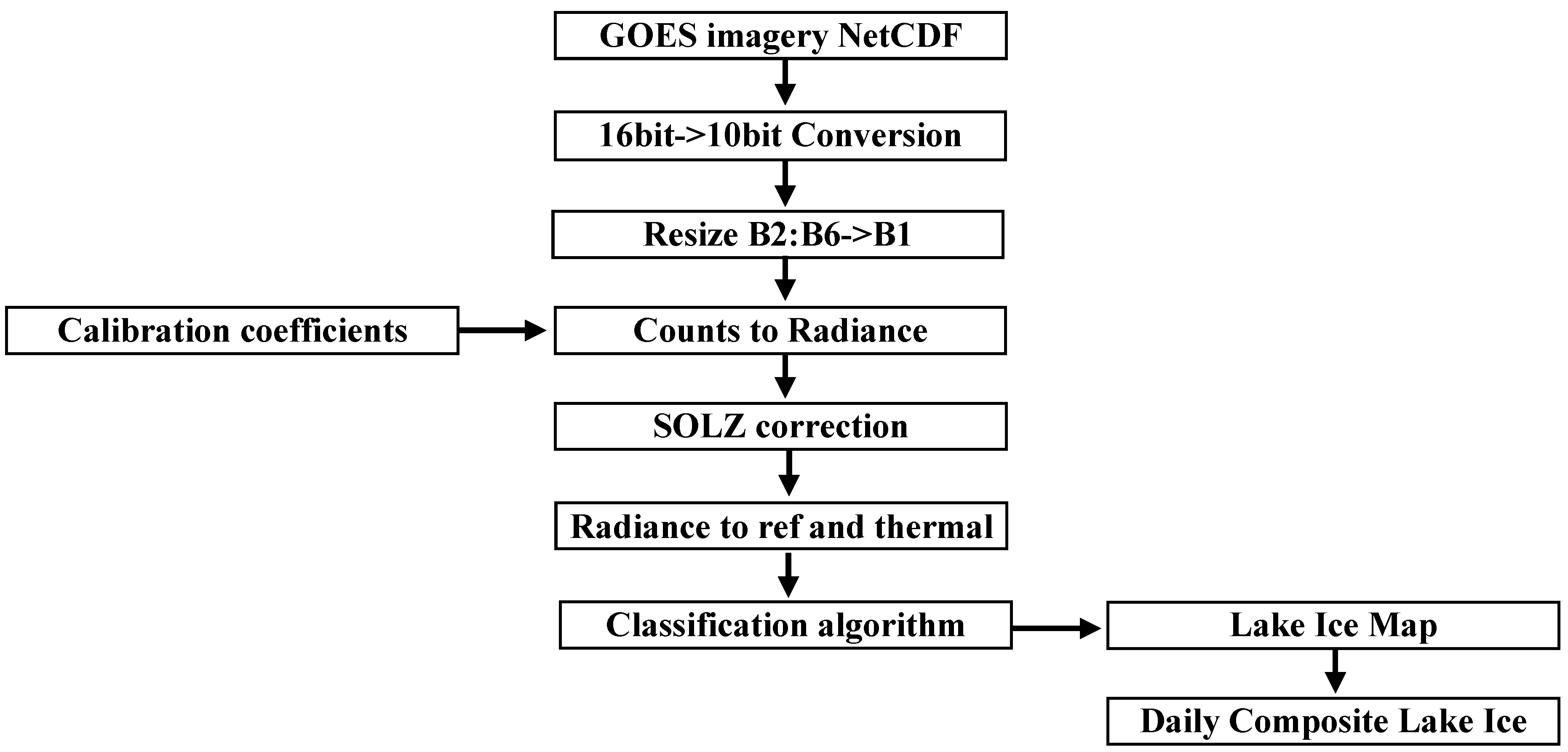
2.2. Approach and Algorithm Development
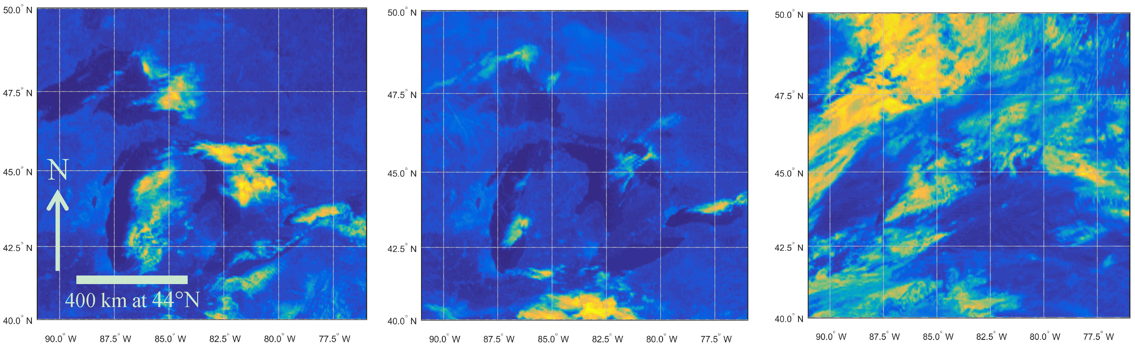
2.2.1. VIS and MIR Reflectance
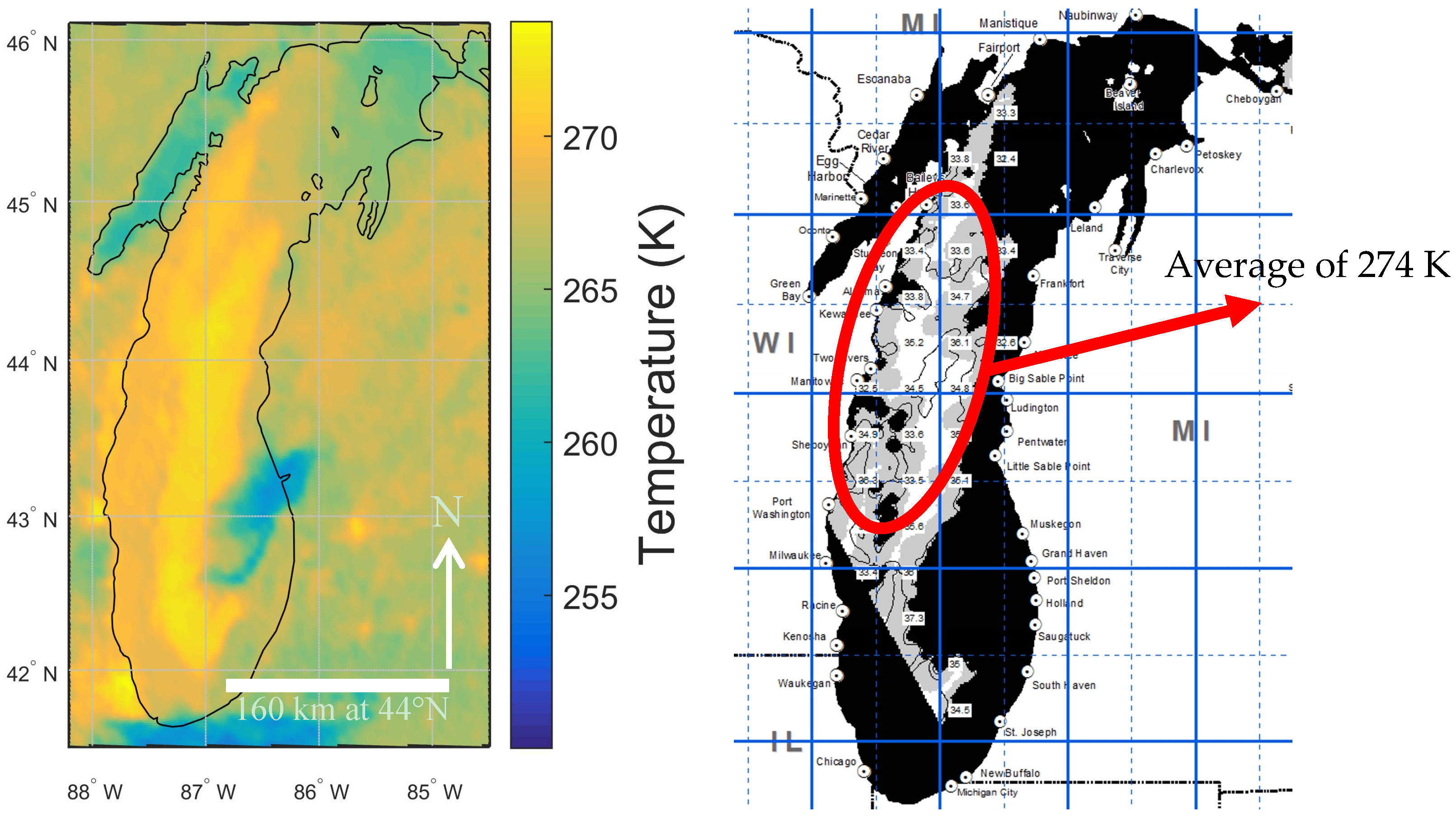
2.2.2. Skin Temperature
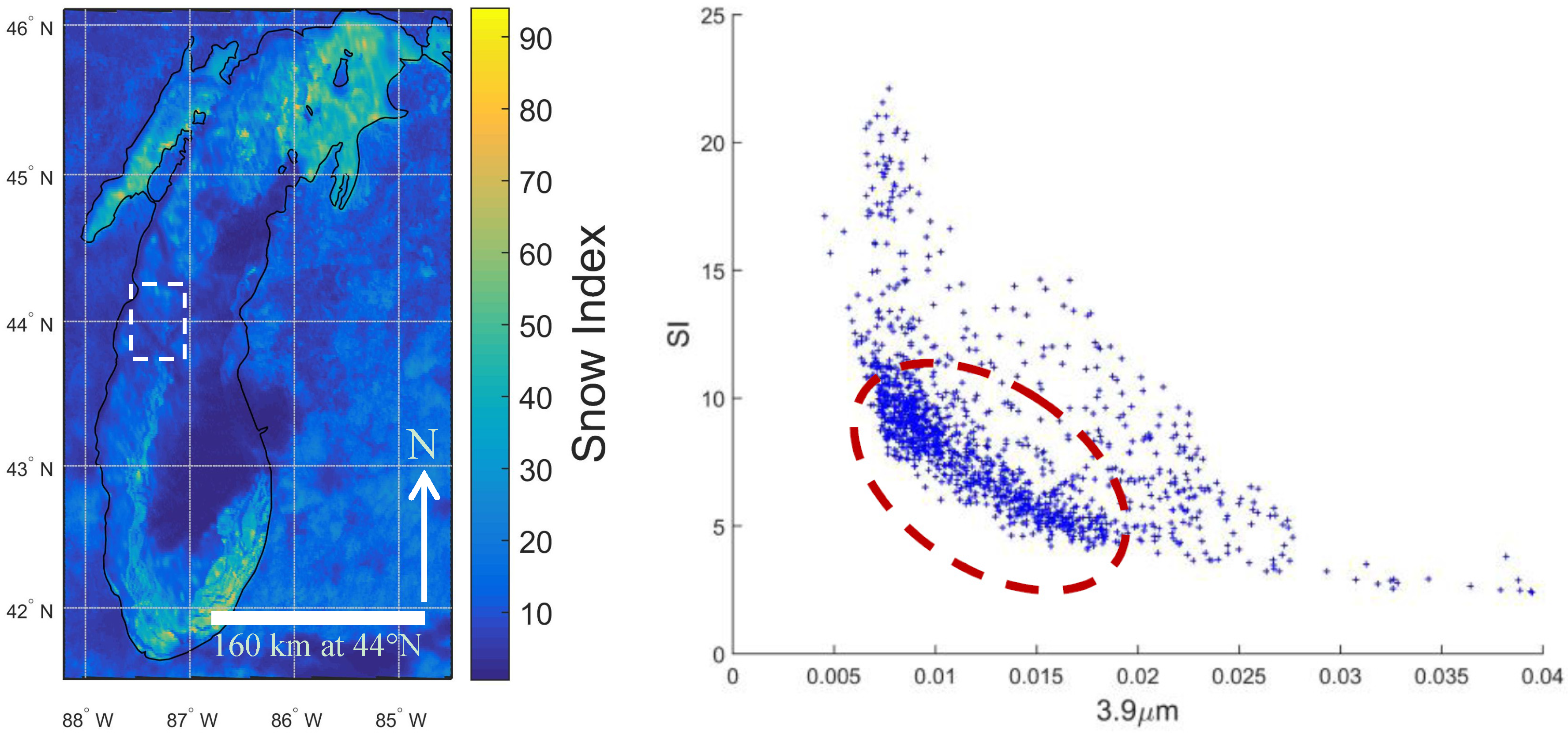
2.2.3. Snow Index
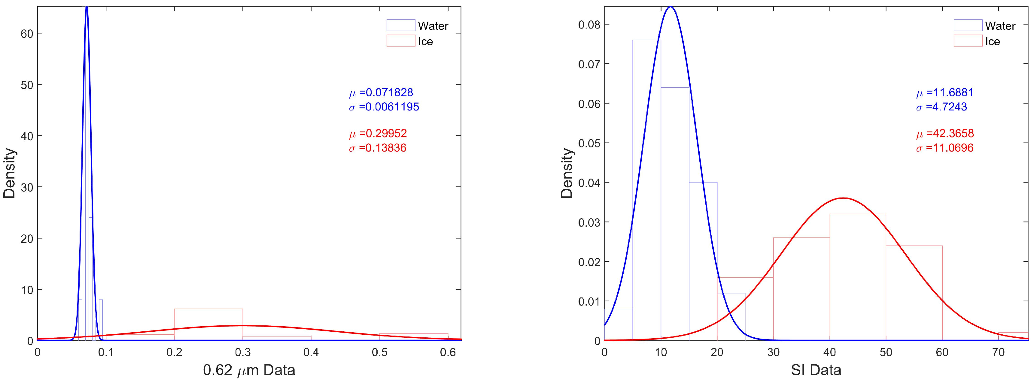
2.2.4. Threshold Determination
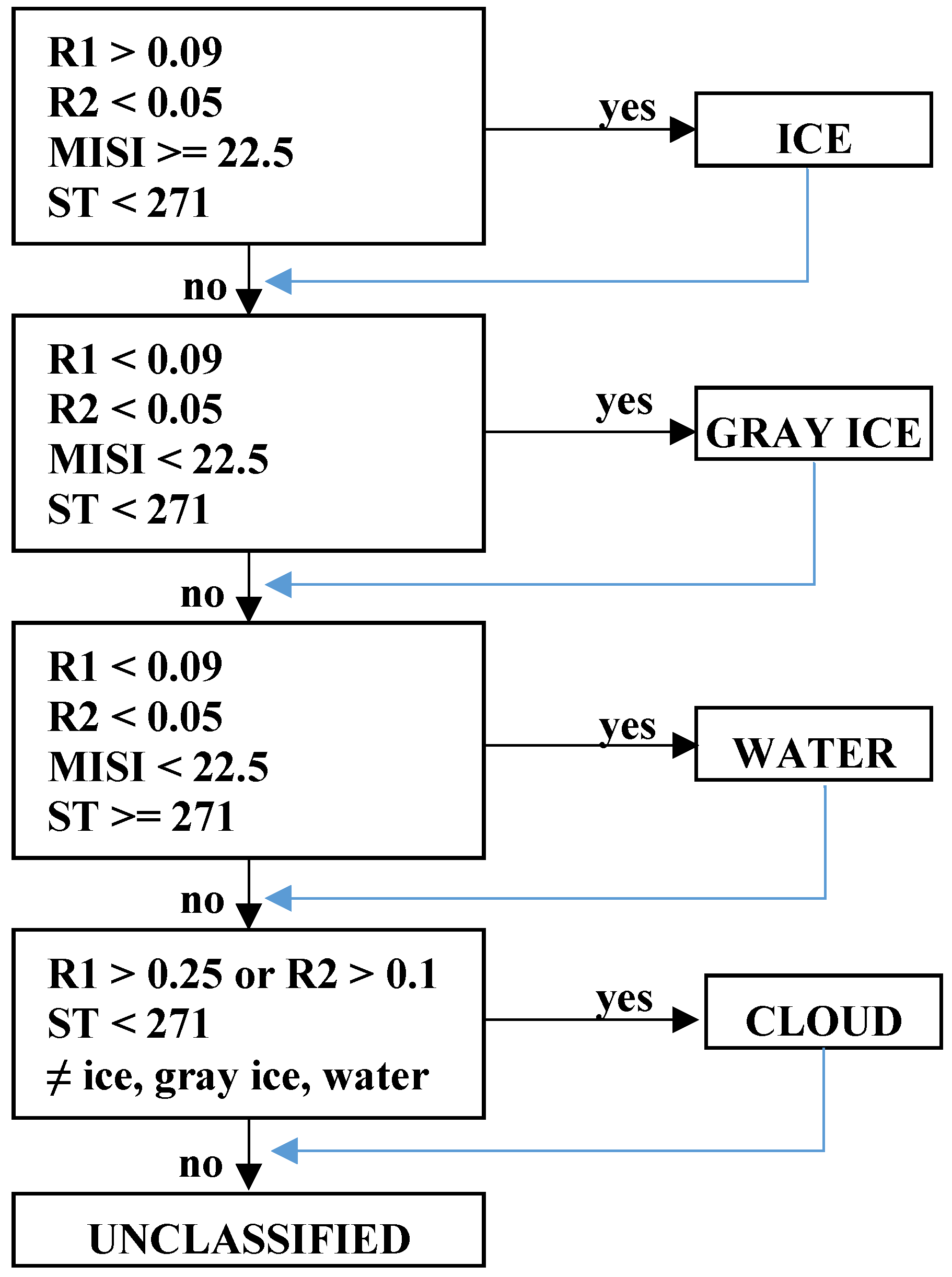
2.2.5. Classification Algorithm
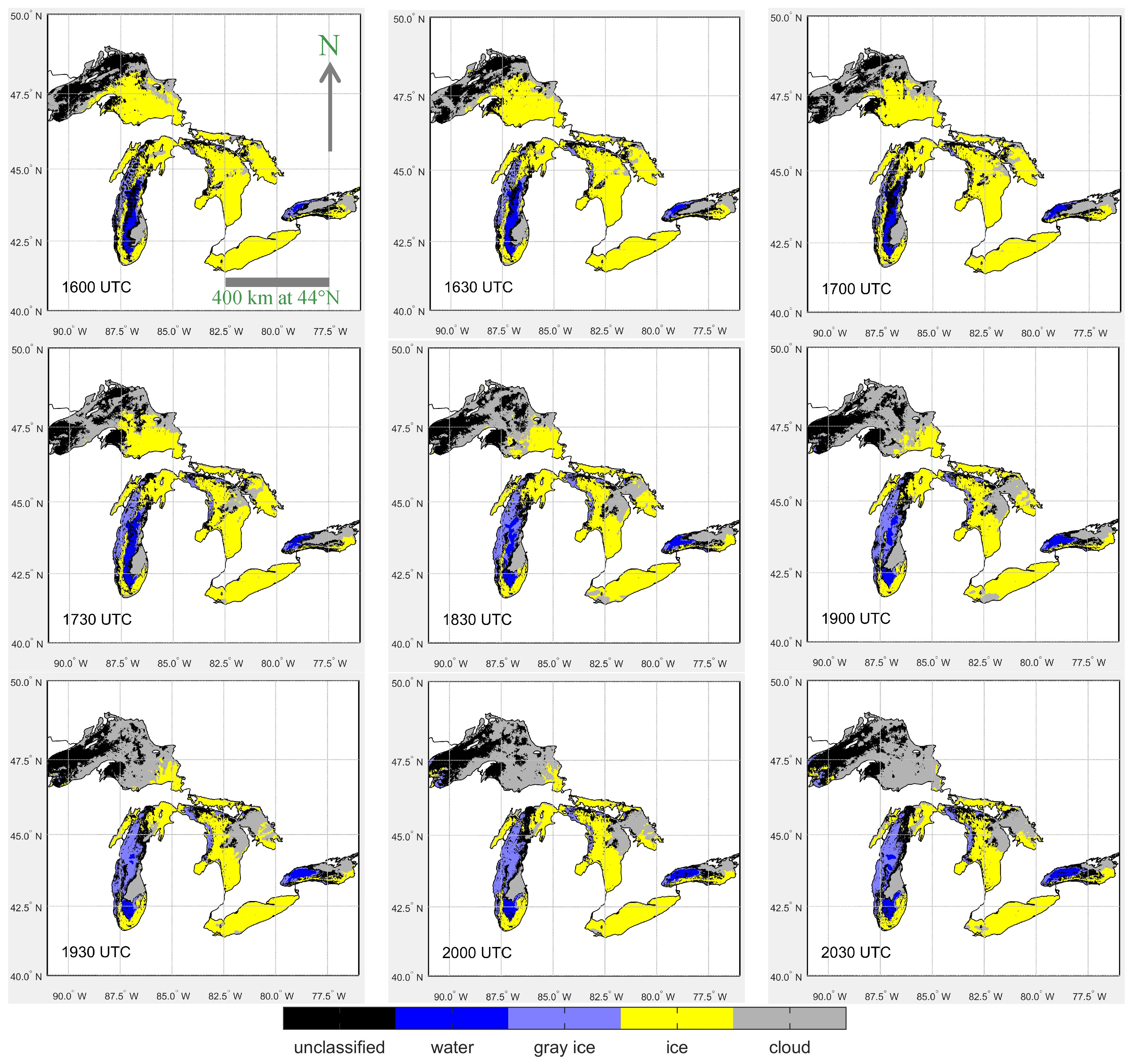
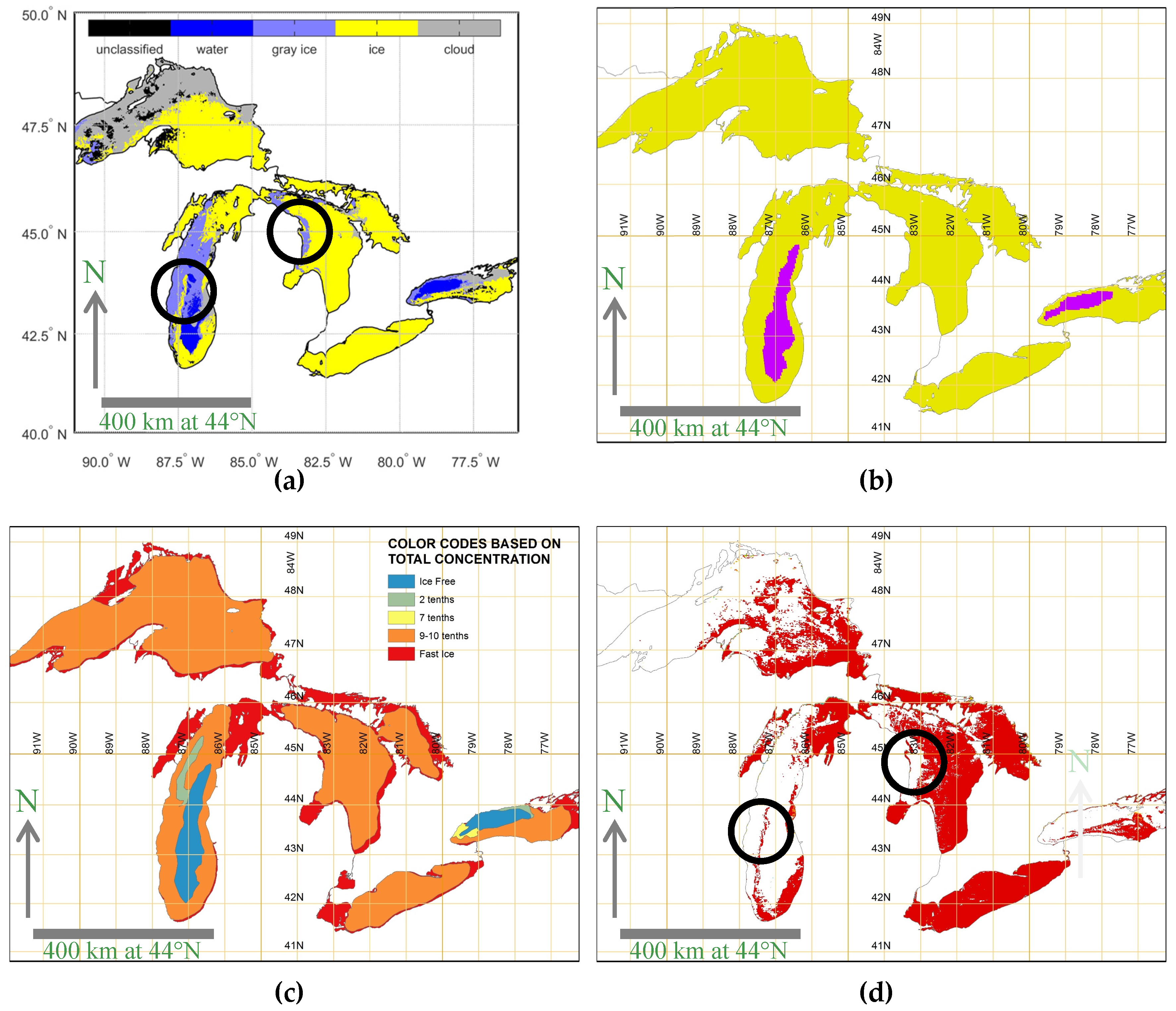
3. Results
4. Conclusions
Acknowledgments
Author Contributions
Conflicts of Interest
References
- National Snow and Ice Data Center. Available online: https://nsidc.org/cryosphere/seaice/characteristics/formation.html (accessed on 1 September 2016).
- Zeng, Q.; Cao, M.; Feng, X.; Liang, F.; Chen, X.; Sheng, W. A study of spectral reflection characteristics for snow, ice and water in the north of China. Hydrol. Appl. Remote Sens. Remote Data Transm. 1984, 145, 451–462. [Google Scholar]
- Salisbury, J.W.; D’Aria, D.M.; Wald, A. Measurements of thermal infrared spectral reflectance. J. Geophys. Res. 1994, 99, 24235–24240. [Google Scholar] [CrossRef]
- Perovich, D.K. The Optical Properties of Sea Ice; No. MONO-96–1; Army Cold Regions Research and Engineering Lab: Hanover, NH, USA, 1996; pp. 8–9.
- Perovich, D.K. The Optical Properties of Young Sea Ice; No. SCIENTIFIC-17; Washington Univ Seattle Dept of Atmospheric Sciences: Seattle, WA, USA, 1979; p. 71. [Google Scholar]
- Perovich, D.K.; Roesler, C.S.; Pegau, W.S. Variability in Arctic sea ice optical properties. J. Geophys. Res. Ocean. 1998, 103, 1193–1208. [Google Scholar] [CrossRef]
- Valovcin, F.R. Snow/Cloud Discrimination; No. AFGL-TR-76–0174; Air Force Geophysics Lab, Hanscom AFB: Bedford, MA, USA, 1976; p. 13.
- Kyle, H.L.; Curran, R.J.; Barnes, W.L.; Escoe, D. A cloud physics radiometer. In Proceedings of the 3rd Conference on Atmospheric Radiation, Boston, MA, USA, 28–30 June 1978; pp. 107–109.
- Dozier, J. Spectral signature of alpine snow cover from the Landsat Thematic Mapper. Remote Sens. Environ. 1989, 28, 9–22. [Google Scholar] [CrossRef]
- Hall, D.K.; Riggs, G.A.; Salomonson, V.V. Development of methods for mapping global snow cover using moderate resolution imaging spectroradiometer data. Remote Sens. Environ. 1995, 54, 127–140. [Google Scholar] [CrossRef]
- Liu, Y.; Key, J.; Mahoney, R. Sea and freshwater ice concentration from VIIRS on Suomi NPP and the future JPSS satellites. Remote Sens. 2016, 8, 523. [Google Scholar] [CrossRef]
- Riggs, G.; Hall, D.K. Snow mapping with the MODIS Aqua instrument. In Proceedings of the 61st Eastern Snow Conference, Portland, ME, USA, 9–11 June 2004.
- Haq, M.A.; Jain, K.; Menon, K.P.R. Development of new thermal ratio index for snow/ice identification. Int. J. Soft Comput. Eng. 2012, 1, 2231–2307. [Google Scholar]
- Allen, R.C., Jr.; Durkee, P.A.; Wash, C.H. Snow/cloud discrimination with multispectral satellite measurements. J. Appl. Meteorol. 1990, 29, 994–1004. [Google Scholar] [CrossRef]
- Key, J.; Barry, R.G. Cloud cover analysis with Arctic AVHRR data: 1. Cloud detection. J. Geophys. Research Atmos. 1989, 94, 18521–18535. [Google Scholar] [CrossRef]
- Romanov, P.; Gutman, G.; Csiszar, I. Automated monitoring of snow cover over North America with multispectral satellite data. J. Appl. Meteorol. 2000, 39, 1866–1880. [Google Scholar] [CrossRef]
- Lee, J.; Chung, C.; Ou, M. Evaluation of the Geostationary Satellite Based Snow and Sea Ice Detection Algorithm; Gisangcheong-gil 45; National Institute of Meteorological Research/Korea Meteorological Administration: Seoul, Korea, 2015.
- European Organization for the Exploitation of Meteorological Satellites (EUMETSAT). MSG Channels. Available online: http://oiswww.eumetsat.org/WEBOPS/msg_interpretation/msg_channels.php (accessed on 1 September 2016).
- Michigan Sea Grant Coastwatch. Lake Michigan Surface Temperature. Available online: http://www.coastwatch.msu.edu/michigan/archive/m/Feb28/2015_Feb28_1254EDT.gif (accessed on 1 September 2016).
- Ghedira, H.; Khanbilvardi, R.; Romanov, P. Development of an advanced technique for mapping and monitoring sea and lake ice for the future GOES-R Advanced Baseline Imager (ABI). In Proceedings of the 2007 IEEE International Geoscience and Remote Sensing Symposium, Barcelona, Spain, 23–28 July 2007.


| GOES-13 Imager | |||||
|---|---|---|---|---|---|
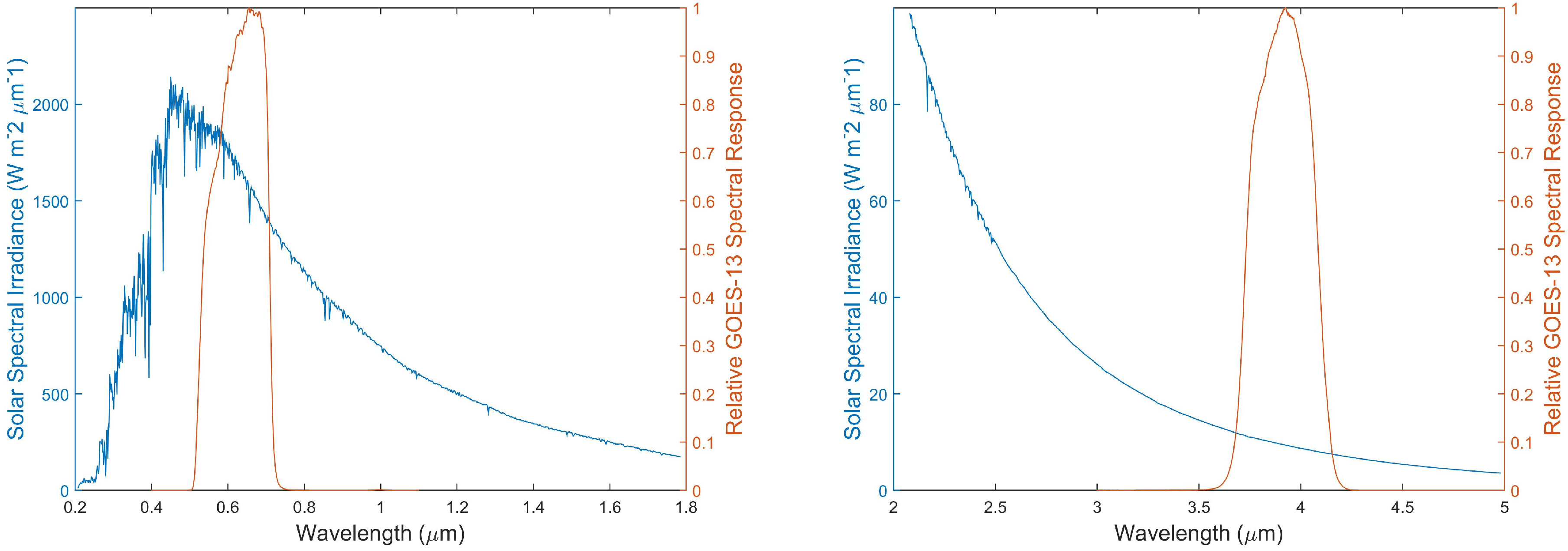
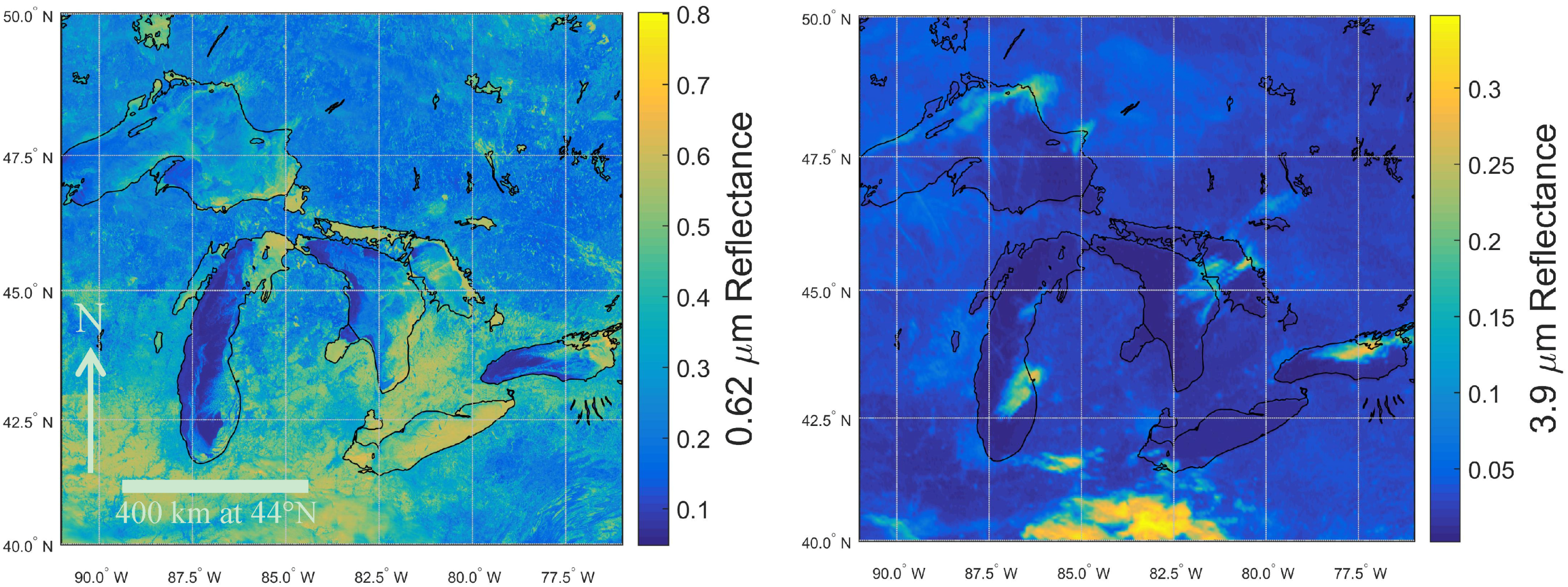
| Channel # | 1 (VIS) | 2 (MIR) | 3 (Moisture) | 4 (IR1) | 6 (IR2) |
| Wavelength Range (µm) | 0.54–0.71 | 3.73–4.08 | 5.90–7.28 | 10.19–11.18 | 13.00–13.71 |
| Central Wavelength (µm) | 0.62 | 3.90 | 6.54 | 10.7 | 13.34 |
| Instantaneous Field of View (IFOV), km | 1 | 4 | 4 | 4 | 4 |
© 2016 by the authors; licensee MDPI, Basel, Switzerland. This article is an open access article distributed under the terms and conditions of the Creative Commons Attribution (CC-BY) license (http://creativecommons.org/licenses/by/4.0/).
Share and Cite
Dorofy, P.; Nazari, R.; And, P.R.; Key, J. Development of a Mid-Infrared Sea and Lake Ice Index (MISI) Using the GOES Imager. Remote Sens. 2016, 8, 1015. https://doi.org/10.3390/rs8121015
Dorofy P, Nazari R, And PR, Key J. Development of a Mid-Infrared Sea and Lake Ice Index (MISI) Using the GOES Imager. Remote Sensing. 2016; 8(12):1015. https://doi.org/10.3390/rs8121015
Chicago/Turabian StyleDorofy, Peter, Rouzbeh Nazari, Peter Romanov And, and Jeffrey Key. 2016. "Development of a Mid-Infrared Sea and Lake Ice Index (MISI) Using the GOES Imager" Remote Sensing 8, no. 12: 1015. https://doi.org/10.3390/rs8121015