Article

Secondary Fault Activity of the North Anatolian Fault near Avcilar, Southwest of Istanbul: Evidence from SAR Interferometry Observations

1
State Key Laboratory of Geodesy and Earth’s Dynamics, Institute of Geodesy and Geophysics, Chinese Academy of Sciences, Wuhan 430077, China
2
GFZ-German Research Centre for Geosciences, Telegrafenberg, Potsdam 14473, Germany
3
e-GEOS—An ASI/Telespazio Company, Via Tiburtina 965, Rome 00156, Italy
4
Department of Geodesy, Kandilli Observatory and Earthquake Research Institute, Boğazici University, Istanbul 34680, Turkey
5
DLR German Aerospace Center, Microwaves and Radar Institute, Weßling 82234, Germany
*
Author to whom correspondence should be addressed.
Remote Sens. 2016, 8(10), 846; https://doi.org/10.3390/rs8100846
Submission received: 12 July 2016 / Revised: 1 October 2016 / Accepted: 11 October 2016 / Published: 18 October 2016

Abstract

:
Strike-slip faults may be traced along thousands of kilometers, e.g., the San Andreas Fault (USA) or the North Anatolian Fault (Turkey). A closer look at such continental-scale strike faults reveals localized complexities in fault geometry, associated with fault segmentation, secondary faults and a change of related hazards. The North Anatolian Fault displays such complexities nearby the mega city Istanbul, which is a place where earthquake risks are high, but secondary processes are not well understood. In this paper, long-term persistent scatterer interferometry (PSI) analysis of synthetic aperture radar (SAR) data time series was used to precisely identify the surface deformation pattern associated with the faulting complexity at the prominent bend of the North Anatolian Fault near Istanbul city. We elaborate the relevance of local faulting activity and estimate the fault status (slip rate and locking depth) for the first time using satellite SAR interferometry (InSAR) technology. The studied NW-SE-oriented fault on land is subject to strike-slip movement at a mean slip rate of ~5.0 mm/year and a shallow locking depth of <1.0 km and thought to be directly interacting with the main fault branch, with important implications for tectonic coupling. Our results provide the first geodetic evidence on the segmentation of a major crustal fault with a structural complexity and associated multi-hazards near the inhabited regions of Istanbul, with similarities also to other major strike-slip faults that display changes in fault traces and mechanisms.

1. Introduction

Crustal strike-slip faults are found to be highly segmented, with patches of high or low slip, and parasitic or associated faults that may sporadically become seismically active [1,2,3] and often localize at geometric bends of the main fault trace [4]. The North Anatolian Fault (NAF) is one of the most active strike-slip faults in the world and can be traced from eastern Turkey to the northern Aegean Sea with a scale of ~1200 km [5]. Near the Almacık block, the NAF separates into two branches, and the northern branch of the NAF (NNAF) continues submarine into the Marmara Sea, aligning with the north and south slopes of the Çınarcık Basin [6] (Figure 1). The strike of the northern branch then bends from the northwest to the west [6]. As we shall discuss in this work, the localization of this geometric bend is also the region of fault complexity near Küçükçekmece Lake, associated with secondary faulting processes that can be observed using synthetic aperture radar (SAR) persistent scatterer interferometry (PSI), a modern space geodetic technique.
The 1999 İzmit/Düzce earthquake disaster highlighted the high seismic hazard and revealed a westward propagation of earthquakes towards the Marmara Sea [10]. The tectonic evolution of the NNAF beneath the Marmara Sea has been widely discussed in past decades; some authors suggest that the NNAF deforms as a single shear zone [11], whereas others suggest that the crust beneath the Marmara Sea is separated by an E-W trending graben [12]. Besides, the evolution of the NNAF zone has also been interpreted as a combination of en-echelon strike-slip faults and pull-apart basins [6,13,14] associated with numerous subparallel fault scarps of unknown activity [7,15]. These investigations mostly focused on the fault activity beneath the Marmara Sea, but the possible activity of secondary faults north of the Marmara Sea remained to be studied. As the faults are shaping the land and directly affect the populated regions of western Istanbul, monitoring the fault activity in this region is of great importance.
Previous studies on seismic and bathymetric observations show evidence of the existence of secondary faults near the two lakes (Büyükçekmece Lake (BL) and Küçükçekmece Lake (KL); Figure 1), north of the Marmara Sea [8,16,17,18,19]. These secondary faults were found to be NW-SE oriented following the geographic alignment of the lake, which also show general consistency with the inland drainage pattern and the scarps of the surrounding terrain [19]. Furthermore, the agreement between the strike and location of the secondary faults and off-shore active faults indicates that the secondary faults near the lakes are not local fault systems, but related to the NW extension of the NNAF [16].
Near-field geodetic observations can provide an independent constraint on the present activity of these secondary faults. Recent GPS observations show local crust deformation (~5 mm/year) near KL [17,20], however, the inferred results may suffer from the spatial limitation of the survey-mode GPS observation. Previous studies [21,22] already described the pronounced subsidence of the Avcilar area (Figure 1), but the horizontal movement related to the secondary fault activity remained to be studied.
In this paper, well-covered long-term PSI measurements were carried out by exploiting the ESA ENVISAT ascending (Track 429) and descending (Track 336) data archive, in order to study the stable near-field crustal deformation (Figure 1). After geometric decomposition and model-based correction of the post-seismic viscoelastic relaxation associated with the 1999 İzmit/Düzce earthquakes, the slip rate and locking depth of the secondary fault beneath KL were determined for the first time based on the assumption of a single dextral fault that was inferred from geological studies [16,17]. We compare our findings to independent information and discuss the implications of these secondary faults, as well as the relationship of the fault slip and fault trend to the geomorphology and landslide activity.

2. Data Handling and Method

Spaceborne SAR interferometry (InSAR) allows investigating the study area at high resolution and identifying subtle deformation occurrences. The basic principles of SAR interferometry have been extensively described in the literature [23,24], and the techniques were then significantly improved by the application of time series procedures. The small baseline subset technique [25] allows such time series analysis and is based on interferograms with small baselines to limit geometric decorrelation and was used to map subsidence zones in the Avcilar area nearby Istanbul [22]. The PSI technique, with the idea of selecting distinct pixels, named persistent scatterers (PS), characterized by a coherent signal over a long series of acquisitions, irrespective of the baseline, brought important advances in the field, allowing millimetric precision of displacement detection [26]. Since then, different PSI and, in general, multi-interferogram InSAR techniques have been developed [25,27,28,29,30,31]. By means of PSI techniques, very long time series, such as available over the study area west of Istanbul, can be processed, and very dense PS measurements can be obtained in spite of temporal and geometrical decorrelation effects.
In this work, an advanced PSI technique named persistent scatterer pair (PSP) [30] was used to process the full ENVISAT archive of SAR data, in order to study aseismic deformations to the west of Istanbul, a region that is located in the vicinity of an important bend of the NNAF.

2.1. SAR Interferometry Processing

The PSP approach was recently proposed [29,30,32] for the identification of PSs in series of full resolution SAR images and the retrieval of the corresponding 3D positions and displacements. Differently from standard PSI techniques, the PSP method relies only on the relative signal in pairs of nearby points, both for identification and analysis of PSs. For this reason, the PSP technique is intrinsically robust to spatially-correlated disturbances (such as atmospheric and orbital artifacts) and does not need a preliminary processing aimed at compensating these contributions to the signal. In addition, deviations from the models of displacement evolution typically used in PSI techniques (for example, due to strong nonlinear evolutions) are mitigated by the PSP approach because close points likely have similar deviations. Against the mentioned advantages, working with arcs requires many more computations than analyzing single points: in fact, N points can form (N − 1) × N/2 different arcs. The PSP approach is based on a complex algorithm designed to find a set of valid (in the sense of the multi-acquisition coherence or analogous parameters) arcs to form a graph with given connectivity and cardinality. The PS points are identified as the nodes of this graph.
The high number of arcs and the high connectivity of the graph guarantee reliable PS identification and accurate PS measurements. Moreover, it makes it possible to fully extract coherent information even from low-intensity SAR signals, even when strongly scattering structures are not present, the sensed signal is weak and the scattering distributed, as in the case of rather smooth surfaces or natural terrains. In this sense, PS are intended in the general sense of scatterers whose backscattering properties persist unaltered over time (at least for the period of interest), as the name suggests, but that can be also fully distributed. In fact, thanks to the higher range resolution and the stricter orbital control, in the recent satellite SAR systems, the interferometric baseline is below the critical limit, and there are no strong spatial decorrelation phenomena.
The redundant information provided by the highly connected PSP graph is conveniently exploited to guarantee more accurate measurements by a recent method for robust phase unwrapping and finite difference integration [33], which are key processing steps in the reconstruction of PS elevations and displacements from InSAR data. The use of a multi-scale decomposition method [34] allows one to perform a global processing approach also in large areas with high PS density, despite the high computational demand required by the exploitation of very redundant information.
The advantages of globally exploiting redundant arcs connecting different pairs of PS can be particularly relevant in order to obtain reliable and accurate measurements when the PS are very sparse, as in the considered region of Istanbul, which is characterized by the presence of water bodies, mountains and large vegetated areas.
For this study, an area of about 600 km2 surrounding KL was analyzed exploiting the ESA ENVISAT ascending (Track 429) and descending (Track 336) data archive. The ascending dataset consisted of 33 images covering the period December 2002–April 2010 and the descending dataset consisted of 32 images covering the period April 2003–September 2010. The images acquired from the ENVISAT ASAR sensor have the following characteristics: strip map image mode, a resolution of 5 m × 25 m per pixel, VV polarization, a nominal incidence angle of 23 degrees and a maximum baseline of 1800 m. The 3-arcsec SRTM DEM was used as an initial guess for the removal of the topographic contribution. During the PSP processing, the elevation information was further refined from the SAR data stack, by estimating in correspondence of each PS the correction to be applied to the input DEM. The PSP (and, in general, PSI) processing makes it possible to reach a metric elevation precision for each PS with ENVISAT data. It is to be noted that the use of a higher resolution DEM as the initial guess could reduce the computational cost of the algorithm, but would not improve the final elevation accuracy of each PS.
For each dataset, the interferograms with respect to the first image of the series were generated (single master interferogram configuration). In fact, when working at full resolution with PSI techniques, there is no added information in the other interferograms (all the possible pairs can be exactly obtained as a linear combination of the single master interferograms). Persistent scatterers are by definition quite insensitive to spatial and spectral decorrelation effects, and large temporal and spatial baseline interferograms can be used, allowing the full exploitation of long time series of acquisitions. The diagrams of the temporal and spatial distribution of SAR images corresponding to the two analyzed datasets are shown in Figure 2.
By using the PSP method, about 240,000 and 200,000 PS points were extracted for the study area in ascending and descending geometries, respectively. Based on the statistical analysis that we performed, the standard deviation of the deformation measurement error is in the order of 3 mm, typically ranging between 1 and 5 mm, depending on the quality of the specific PS and on the type of ground cover, whereas the refined height measurements have a metric accuracy. The average measurement density is 100 PS/km2 over the whole area and reaches 1000 PS/km2 in the most urbanized areas.

2.2. Signal Decomposition

Due to the radar viewing geometry, ENVISAT observations are ~3-times more sensitive to vertical motion than to fault-parallel motion in this area, assuming a fault trend of N30°W and a strike-slip motion. Previous investigations show that the Avcilar district underwent clear subsidence [21,22]; this signal can overwhelm the horizontal motions induced by fault movement. In order to investigate the particularities of these deformations, we apply a signal decomposition approach that we designed for investigations related to the N30°W striking fault slip. By combining ascending and descending PS-InSAR observations, the LOS (line of sight) velocities can be projected onto any desired set of two orthogonal basis vectors under the assumption that the third component is zero [35]. Such an approximation is particularly suitable for areas around the middle of a straight fault segment as in the present case.
The time-series data of the study region suggest vertical, but also significant horizontal displacement components. In order to improve the signal-to-noise ratio, we estimate the mean LOS velocity between 2002 and 2010. Then, we projected the obtained ascending and descending LOS velocities (Figure 3) onto motions in the fault-parallel and vertical direction using a least square method [35,36]. A uniform fault-parallel direction of horizontal movement was assumed, whereas the fault-perpendicular horizontal component was not considered in the modelling. This horizontal strike-slip motion was already independently inferred from the GPS observation in this area [37], agreeing with the orientation of the KL fault that was shown by seismic investigation [18], as well as by structural studies [16].
The decomposed horizontal and vertical movement are shown in Figure 4a,b. Clear relative movement in the fault-parallel direction was observed on two sides of the KL fault, which agrees well with the tectonic background (dextral character) of this fault. We found that relative horizontal movements striking N30°W locally exceed 5.0 mm/year. This deformation pattern is in good agreement with horizontal velocities from GPS data (see Figure 4a). The quantitative comparison between the horizontal GPS velocity and the inverted horizontal InSAR velocity is shown in Figure A1, from which we can see that the InSAR velocities are generally comparable with that of the GPS observation in terms of magnitude and direction, though a difference is found on a few stations. Note that the inverted horizontal InSAR velocities on two continuous stations (AVCT and KCEK in Figure A1) fit well with that of the GPS observation. Furthermore, clear subsidence was observed in two areas (Figure 4b): the large one is located at the west of KL aligning along a pronounced valley; the small one is located at the east of the lake fault. Subsidence along KL thus is associated with the steep topography and clearly associated with the steeper slopes. Subsidence east of KL, in turn, is found on a relatively flat plain.

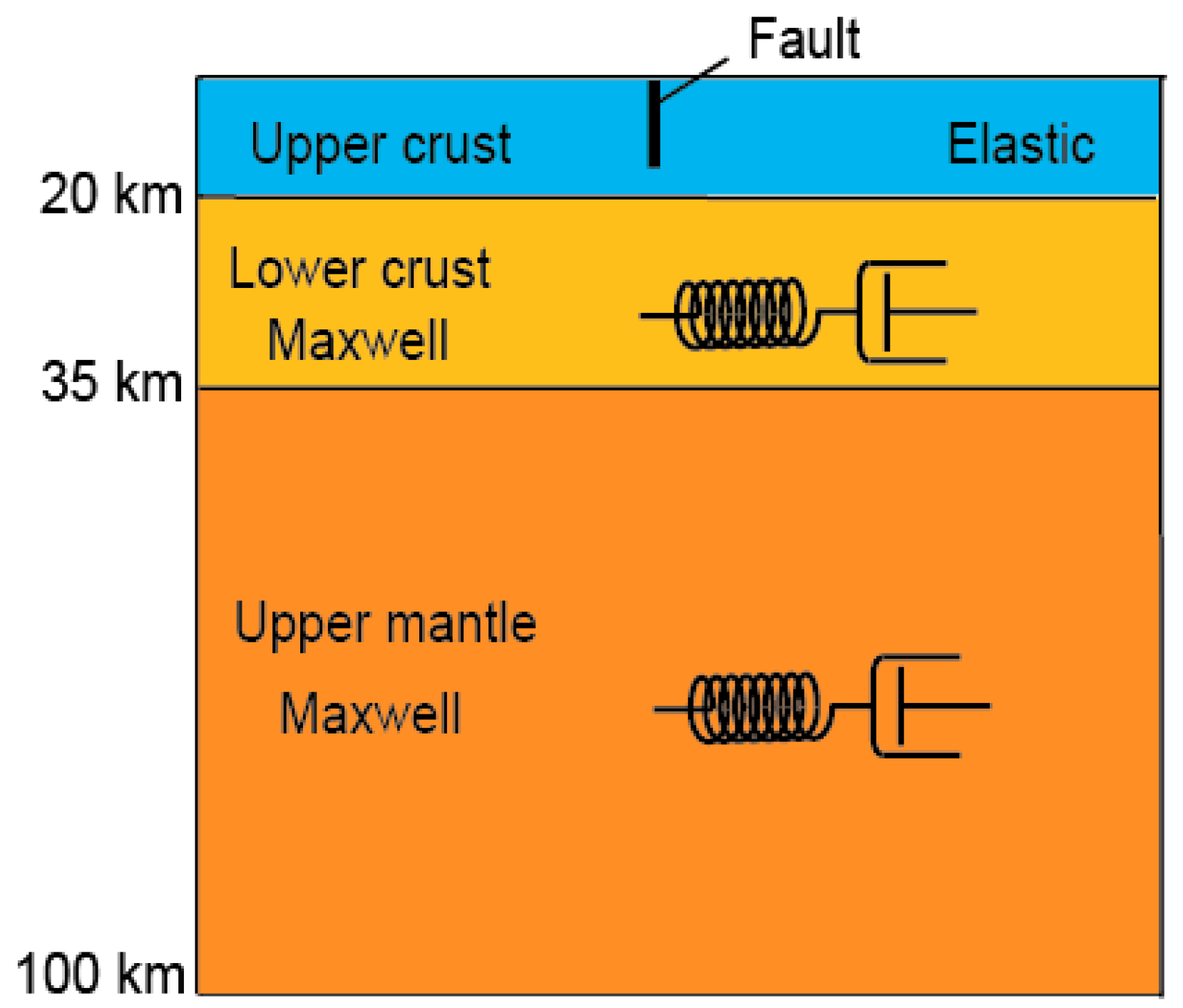
3. Effect of Post-Seismic Viscoelastic Relaxation

The post-seismic viscoelastic relaxation effect (PVRE) may affect crustal deformation near large earthquakes for decades [38]. Studies on post-seismic deformation of the 1999 İzmit/Düzce earthquakes suggest that the PVRE induced by these events is clear and should not be ignored in the PS-InSAR observation period [39]. In this paper, we estimated and removed the PVRE using a model-based method following [40]. The detailed model construction and PVRE estimation have been given in [40], and some key steps are described in this section.
Firstly, a three-layer viscoelastic model was set up to forward simulate this viscoelastic effect on each PS-InSAR point within the observation period (Figure 5). The model has one elastic upper crust layer and two viscoelastic layers representing the lower crust and upper mantle, for which the Maxwell rheology was applied (Figure 5).
Secondly, the lower crust and upper mantle viscosity of the Maxwell rheology play an important role in estimating the PVRE effect [38]. These parameters were inferred from the post-seismic GPS observation in a similar time period by employing a grid-search method [40].
Thirdly, we calculated the PVRE at each PS-InSAR data point using the derived optimal viscosity parameters and the numerical code provided by [41]. The results show that the mean PVRE effect on ground velocity is almost constant in the observation period. Using the optimal viscosities, the calculated PVRE is estimated to be ~2 mm/year horizontally in the study area and is therefore considerable for inverting the fault movement (Figure 4c,d). However, the PVRE reveals a smooth spatial pattern in the area around the KL fault, so that its influence on the estimation of the fault slip is not so significant.
At last, we removed the PVRE from the InSAR velocities, in order to obtain the deformation signal that is largely free of the post-seismic effect (Figure 4e,f).
To avoid the effects induced by other local deformation processes (landsliding, groundwater extraction and others), we low-pass filtered the data using a simple median filtering method. We got the velocity of each InSAR point by calculating the mean value of neighboring points within a distance (filtering length). After filtering the small-scale signal, the relative fault movement becomes more visible (Figure 6), which highlights the relative motions of the KL fault. Other small-scale processes may slightly affect the deformation pattern and play a secondary role in controlling the crustal deformation in this area.

4. Modelling and Results

After removing the PVRE, a velocity profile perpendicular to the fault orientation was constructed (Figure 7), which was used to estimate the fault slip rate and locking depth based on a widely-used 2D screw dislocation model [42]. In this model, the fault-parallel velocity ( v ) as a function of its perpendicular distance to the fault ( x ) can be drawn by:
v ( x ) = ( V / π ) × arctan ( x / D )
where V and D are the slip rate and the locking depth of the KL fault, respectively. A grid-search method was applied to search for the slip rate and locking depth over ranges of 0.5–20 mm/year and 0.5–20 km with 0.5-mm/year and 0.5-km intervals. The RMS (root mean square) misfit between the model and observation for each combination of the parameters was calculated, from which the optimal values of the slip rate and locking depth were fixed by minimizing the RMS misfit.
The uncertainty of the obtained optimal slip rate and locking depth were estimated statistically using the Monte Carlo method [43]. We firstly constructed the 1D variance-covariance matrix of the ascending and descending InSAR data using the method of [44] and generated spatially-correlated noise. Secondly, we obtained the perturbed dataset by adding the noise to the observation. Finally, we searched for optimal parameters based on each disturbed dataset and could analyze the best-fitting model. We run these steps 500 times in order to obtain a robust estimation about the uncertainty of the parameters. The distribution of the slip rate and locking depth are inferred from a Monte Carlo simulation and show a general consistence with the RMS misfit map (Figure 8). The result statistically reveals a mean slip rate of 5.1 ± 0.4 mm/year and a locking depth of 1.0 ± 0.5 km (the mean value and the one-sigma uncertainty; Figure 8), suggesting that the KL fault is active with a shallow locking depth. Therefore, a tectonically and potentially seismically active fault is located in the immediate vicinity of western Istanbul, with important implications as discussed in the following section.
In order to test the effect of possible small-scale deformations (such as landsliding), we also inverted the low-pass filtered data using the same method mentioned above. As shown in Figure 8, we found that similar results as those inverted from the unfiltered data could be obtained, although the data misfits became smaller as the filtering length increasing. The estimated locking depths tend systematically to a very small value (<1 km), suggesting possible creep of this secondary fault. Similar fault creep and shallow locking depth have been found on other strike-slip fault, such as the central section of the San Andreas fault [45] and western sections of the NAF [46].

5. Discussion and Implications

5.1. Limitations

A number of limitations of the present study need to be discussed that may affect the interpretation and correct understanding of our results. Although the herein used PS-InSAR technique provides very robust results at a pixel resolution that is higher than hitherto presented results in the region, the signal investigated is still rather small. Horizontal motions in the sub-centimeter scale are very challenging to observe, which is why we have decided to exploit the average velocity rather than certain time-dependent increments of the data. The advantage of this approach is that the total displacement values become significant. The disadvantage is that temporal variations may not be interpreted. The strong seasonality of the subsidence region [22] or the temporal variations of the landslides [17] are not discussed, as is the nature of the strike-slip fault motion. In this, we cannot decipher if this inferred fault slip is a short-term behavior or a long-term process, warranting further studies. Furthermore, future studies may use the temporal variability of the different processes to investigate the different types of deformation (faulting, landsliding and subsidence).
In addition, compared with the descending data, the ascending data are less sensitive to the horizontal movement of the KL fault due to the geometric setting. This limitation may highly affect the extraction of horizontal motion if only the descending data are available. In this paper, owing to the combined analysis of the ascending and descending data, such an effect would be decreased to a certain degree. Synthetic tests were carried out in order to investigate how the horizontal and vertical deformation signal depend on the geometric setting of the ascending, descending data and the fault orientation. As the results show in Figure A2, Figure A3, Figure A4 and Figure A5, we find that the input horizontal and vertical signals can generally be well recovered with the geometric setting of the InSAR data and the fault orientation in this area. Nevertheless, more close investigations, such as continuous cross-fault GPS and strain-meter observation, are strongly required in order to obtain a more robust estimation of the fault movement.
This study is based on assumptions made from earlier studies on the KL fault mechanism. In addition, it is hard to further distinguish whether the KL fault is a simple fault or a narrow zone including a few small active faults [18] using the geodetic data shown in this paper. We assumed it to be a single dextral fault as a first order approximation.

5.2. Tectonic Implication

Geodetic results in this paper show clear dextral movement of the fault near KL, revealing the movement of an active secondary fault north of the Marmara Sea. Our results of relative motion (~5 mm/year) on the two sides of KL provide an important indication of the existence of the secondary faults in this area. Combined with previous geological and seismic results [8,16,17,18,19], this active fault perhaps can be interpreted as an extension of the northern branch of the NAF (NNAF) [16,18]. This interpretation suggests two possibilities about the evolution of the north branch of the NAF: one is that the NNAF does not bend from NW to WSW at KL and connect to the Ganos fault at the west, but extends to KL northwest [16]; the other one is that the NNAF might separate into two branches, one running northwest into the KL and the other one bending to the WSW direction.
For detailed analysis of the two possibilities, more close observations, such as more dense near-field GPS [36] and numerical simulations [47], are required. However, no matter which possibility reveals the development of the north branch of the NAF, the active fault beneath KL would play an important role in regional tectonic evolution and related seismic hazard assessment.
Fault complexities at fault bends are observed worldwide. These are commonly explained by perturbations induced by geometrical complexities in a main fault trace [4]. During multiple earthquake cycles residual stresses may accumulate and lead to the formation and dislocation of secondary faults. Whether the herein investigated N30°W trending fault on land is seismogenically active is not known. However, due to the shallow locking depth shown by our modelling result, the KL fault might be subjected to aseismic creep. This perhaps can explain that only a few earthquakes were observed in this area [48].

5.3. Local Landslides and Subsidence

Faulting processes are often associated with topography reshaping, steep erosion and landslide processes. Many small-scale landslides have been observed in the Avcilar area (upper left panel in Figure 1), which may affect the local deformation process. Landslide inventory maps of that region suggest steeper slopes to be vulnerable for flank instability. For this reason, one may suspect that the observed horizontal PS-InSAR deformation might be induced by slow landslides. Many factors can affect the development of landslides, where the terrain gradient has a dominant role in controlling the susceptibility and the final movement [9,49]. In other words, if the observed motions in this area mainly result from the landslides, they should show general spatial correlation with the terrain gradient.
With this assumption, we decomposed the LOS velocities into N120°W and vertical directions using the method mentioned in Section 2.2, where the N120°W direction is close to the horizontal component of the maximum terrain gradient in this area. We then draw the decomposed horizontal velocities along the selected profile and compared them with the corresponding terrain. As shown in Figure 9, no clear spatial correlation was found between the horizontal motion and the slope of the terrain, even when filtered data were applied. We thus conjecture that the modelled long-term N30°W PS-InSAR velocity is distinct from that of the local landslides, but mainly induced by stable tectonic movement.
The subsidence area at the west of the KL fault agrees well with the results of [21] in terms of location and subsidence rate; however, our result suggests that this subsidence shows also a high spatial correlation with the Haramidere valley, which perhaps was induced by ground water redistribution [21], soli liquefaction [50] or other unknown mechanisms, which deserve future investigations. The subsidence area east of the KL fault is thought to be mainly related to substratum material consolidation processes, as well as the human activity of this rapidly growing urban area [22].

6. Conclusions

In this paper, we use long-term PS-InSAR observation (2002–2010) to investigate crustal deformation and related secondary fault activity southwest of Istanbul. The mean LOS velocity in ascending and descending geometries was decomposed into fault-parallel and vertical direction motions, in which the post-seismic viscoelastic relaxation effect of the 1999 İzmit/Düzce earthquakes was removed based on model-based estimations. Based on the assumption of the fault behavior (i.e., fixed fault orientation and strike-slip character) inferred from geological studies, our results suggest that a secondary fault near KL is now active with a dextral slip rate of ~5 mm/year and a shallow locking depth of <1.0 km. The results show the first geodetic evidence about the existence and present activity of secondary faults north of the Marmara Sea, which has valuable implications for regional tectonic evolution and close seismic hazard assessment of the mega city Istanbul.

Acknowledgments

We thank the editor and the reviewers for their insightful comments. This work is supported by the National Natural Science Foundation of China (Grant Numbers 41304017, 41674023 and 41274104) and the New Directions in Seismic Hazard Assessment through Focused Earth Observation in the Marmara Supersite (MARSite) project co-funded by the European Commission within the Seventh Framework Programme (Grant No. 308417). Data processing and analysis were made as a contribution to the European Space Agency (ESA) Scientific Exploitation of Operational Missions (SEOM) project Sentinel-1—INSAR performance study with TOPS data (INSARAP, ESA-ESRIN Contract 4000110587/14/I-BG), and to the Helmholtz Alliance on Remote Sensing and Earth System Dynamics (EDA).

Author Contributions

F.D. and T.R.W. contributed to the data analysis, modeling and manuscript writing. F.M. and M.C. contributed to the InSAR data processing. R.W., S.E., X.X. and P.P. contributed to the result analysis and manuscript revision. All authors reviewed the manuscript.

Conflicts of Interest

The authors declare no conflict of interest.

Appendix A

A.1. Quantitative Comparison between GPS and InSAR Observation

Figure A1 shows the comparison between the GPS observation and the InSAR observation. We projected the horizontal GPS velocity onto the N30°E direction and find that the horizontal InSAR velocities are generally comparable with those of the GPS observation in terms of magnitude and direction, though a difference is found for a few stations. Note that the inverted horizontal InSAR velocities on two continuous stations (AVCT and KCEK in Figure A1) fit well with that of the GPS observation.
Figure A1. Comparison between the obtained InSAR velocity and the observed GPS velocity in the study area. The observed horizontal GPS velocities (black arrows) were projected onto the N30°E direction (red arrows). The horizontal InSAR velocity (blue arrows) on each GPS station was the average value of InSAR points within 1 km surrounding the GPS site. AVCT and KCEK are continuous stations, and others are survey sites.
Remotesensing 08 00846 g010

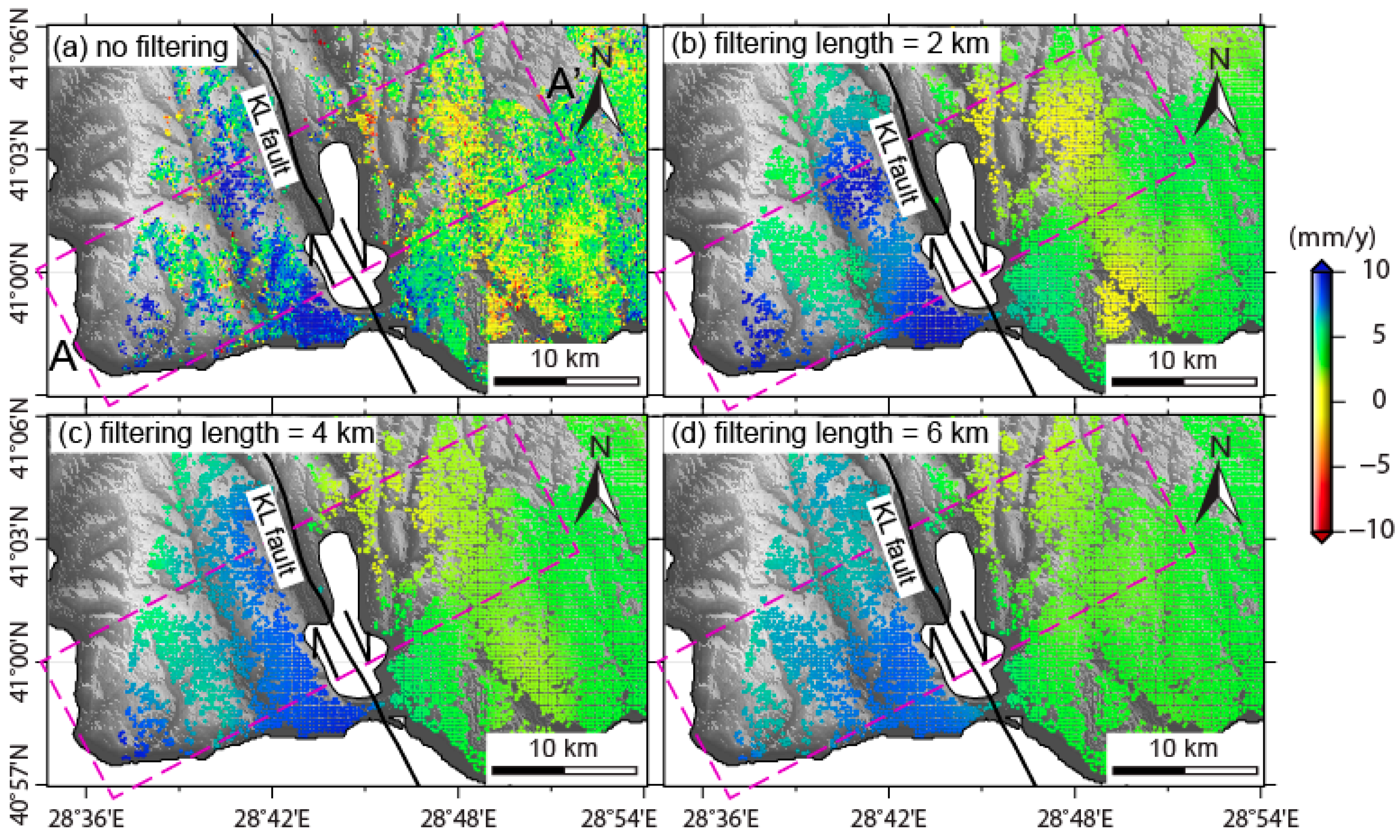
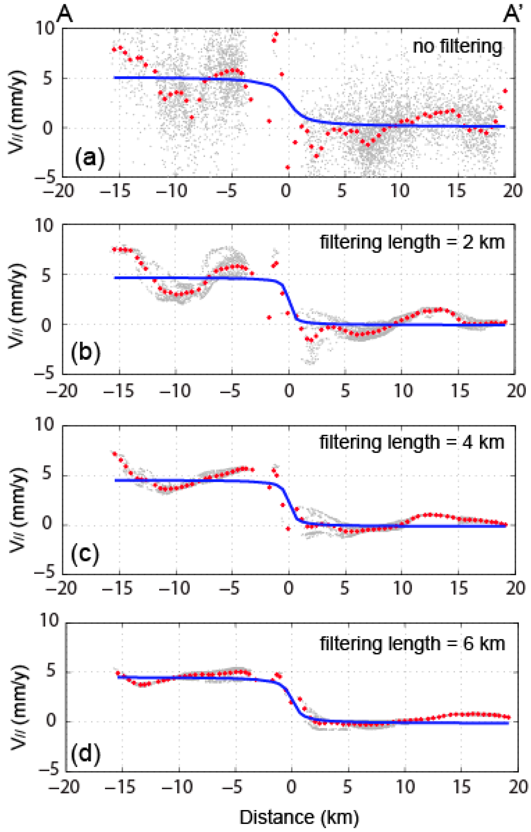
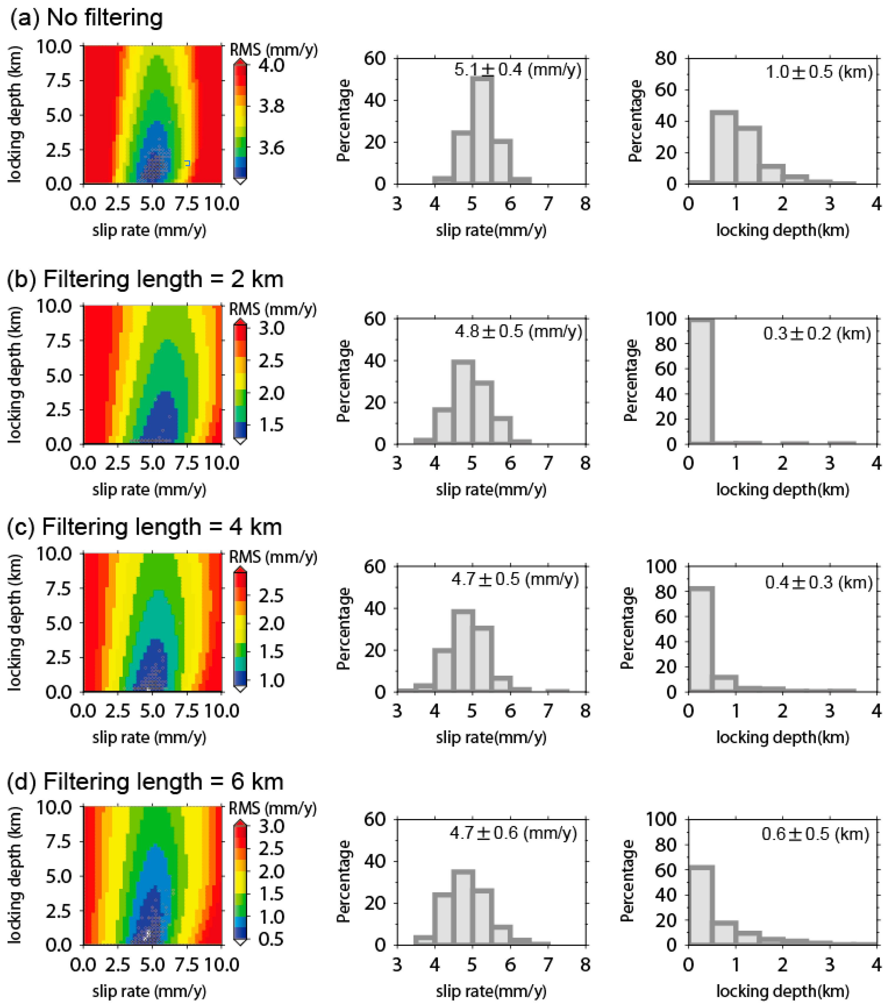
A.2. Synthetic Tests

Synthetic tests were carried out in order to investigate how the horizontal and vertical deformation signals depend on the geometric setting of the ascending and descending data and the fault orientation. The steps are as follows:
We firstly assumed a right lateral slip rate of 5 mm/year of the KL fault (locking depth = 0) and generate the horizontal velocity field (Figure A2a). Two rectangular subsidence areas with a vertical velocity of −5 mm/year (Figure A2b) were added to the horizontal velocity field.
Secondly, we projected the velocity field that was obtained in the first step to the LOS directions of the ascending track and descending track (Figure A2c,d).
Thirdly, we added noise to the generated LOS velocities (Figure A2e,f). A Gaussian noise with a standard deviation of 2 mm/year was used here.
Fourthly, we inverted the LOS velocities to get the horizontal and vertical velocities on each point (Figure A2g,h) using the least square method that was mentioned in Section 2.2.
At last, we low-pass filtered the obtained horizontal and vertical field to remove the high-frequency signals as has been done in the main text. A filtering length of 1 km is used here, but similar results can be obtained with filtering lengths of 2 km and 3 km (as shown by Figure 6). The detailed comparison of the input and the recovered horizontal signal along the selected profile was shown in Figure A3.
Other Gaussian noise levels (e.g., with standard deviations of 1 mm/year and 3 mm/year) were also tested, and a similar result can be obtained. In addition, we also used the random spatially-correlated noise generated from the variance-covariance matrix (as mentioned in Section 4) instead of the Gaussian noise in the synthetic test, and similar results can be obtained (Figure A4 and Figure A5).
From the synthetic tests, we find that the input signal can generally be well recovered with the geometric setting of the InSAR data and the fault orientation in this study.
Figure A2. Synthetic data that was used for the test. (a,b) Synthetic horizontal ((N30°W) and vertical velocity fields; (c,d) Generated LOS velocity fields in the ascending and descending geometric setting; (e,f) Inferred from (c,d) by adding noise; (g,h) Horizontal and vertical velocity that were inverted from noised synthetic LOS velocities (e,f); (i,j) Low-pass filtered horizontal and vertical velocity field (with a filtering length of 1 km) that were obtained from (g,h).
Remotesensing 08 00846 g011
Figure A3. Input (black dot) and recovered (red dot) horizontal velocity (N30°W) on profiles perpendicular to the orientation of the fault (Figure A2a,i).
Remotesensing 08 00846 g012
Figure A4. Similar to Figure A2, but for the synthetic test using the spatially-correlated noise instead of the Gaussian noise. (a,b) Synthetic horizontal ((N30°W) and vertical velocity fields; (c,d) Generated LOS velocity fields in the ascending and descending geometric setting; (e,f) Inferred from (c,d) by adding noise; (g,h) Horizontal and vertical velocity that were inverted from noised synthetic LOS velocities (e,f); (i,j) Low-pass filtered horizontal and vertical velocity field (with a filtering length of 1 km) that were obtained from (g,h).
Remotesensing 08 00846 g013
Figure A5. Input (black dot) and recovered (red dot) horizontal velocity (N30°W) on profiles perpendicular to the orientation of the fault (Figure A4a,i). Similar to Figure A3, but using the spatially-correlated noise instead of the Gaussian noise in the synthetic test.
Remotesensing 08 00846 g014

References

  1. Segall, P.; Pollard, D.D. Mechanics of discontinuous faults. J. Geophys. Res. 1980, 85, 4337–4350. [Google Scholar] [CrossRef]
  2. Ben-Zion, Y.; Rice, J.R. Slip patterns and earthquake populations along different classes of faults in elastic solids. J. Geophys. Res. 1995, 100, 12959–12983. [Google Scholar] [CrossRef]
  3. Zabcı, C.; Sançar, T.H.; Akyüz, S.; GçKıyak, N. Spatial slip behavior of large strike-slip fault belts: Implications for the Holocene slip rates of the eastern termination of the North Anatolian Fault, Turkey. J. Geophys. Res. Solid Earth 2015, 120, 8591–8609. [Google Scholar] [CrossRef] [Green Version]
  4. Saucier, F.; Humphreys, E.; Weldon, R. Stress near geometrically complex strike-slip faults: Application to the San Andreas fault at Cajon Pass, southern California. J. Geophys. Res. 1992, 97, 5081–5094. [Google Scholar] [CrossRef]
  5. Şengör, A.M.C.; Tuysuz, O.; Imren, C.; Sakınç, M.; Eyidoğa, H.; Görür, N.; Le Pichon, X.; Rangin, C. The North Anatolian fault: A new look. Annu. Rev. Earth Planet. Sci. 2004, 33, 1–75. [Google Scholar] [CrossRef]
  6. Armijo, R.; Meyer, B.; Hubert, A.; Barka, A. Westward propagation of the North Anatolian Fault into the northern Aegean: Timing and kinematics. Geology 1999, 27, 267–270. [Google Scholar] [CrossRef]
  7. Armijo, R.; Pondard, N.; Meyer, B.; Uçarkus, G.; de Lépinay, B.M.; Malavieille, J.; Dominguez, S.; Gustcher, M.; Schmidt, S.; Beck, C.; et al. Submarine fault scarps in the Sea of Marmara pull-apart (North Anatolian Fault): Implications for seismic hazard in Istanbul. Geochem. Geophys. Geosyst. 2005, 6, Q06009. [Google Scholar] [CrossRef]
  8. Gokasan, E.; Ustaomer, T.; Gazioglu, C.; Yucel, Z.Y.; Ozturk, K.; Tur, H.; Ecevitoglu, B.; Tok, B. Morpho-tectonic evolution of the Marmara Sea inferred from multibeam bathymetric and seismic data. Geo-Mar. Lett. 2003, 23, 19–33. [Google Scholar] [CrossRef]
  9. Duman, T.Y.; Çan, T.; Ulusay, R.; Keçer, M.; Emre, Ö.; Ateş, Ş.; Gedik, İ. A geohazard reconnaissance study based on geoscientific information for development needs of the western region of İstanbul (Turkey). Environ. Geol. 2005, 48, 871–888. [Google Scholar] [CrossRef]
  10. Lorenzo-Martin, F.; Roth, F.; Wang, R. Elastic and inelastic triggering of earthquakes in the North Anatolian Fault zone. Tectonophysics 2006, 424, 271–289. [Google Scholar] [CrossRef]
  11. Şengör, A.M.C.; Gorur, N.; Saroglu, F. Strike-slip faulting and related basin formation in zones of tectonic escape: Turkey as a case study. Soc. Ecol. Paleontol. Mineral. Spec. Publ. 1985, 37, 228–264. [Google Scholar]
  12. Smith, A.D.; Taymaz, T.; Oktay, F.Y.; Yuce, H.; Alpar, B.; Basaran, H.; Jackson, J.A.; Kara, S.; Simsek, M. High-resolution seismic profiling in the Sea of Marmara (Northwest Turkey): Late Quaternary sedimentation and sea-level changes. Geol. Soc. Am. Bull. 1995, 107, 923–936. [Google Scholar] [CrossRef]
  13. Wong, H.K.; Ludmann, T.; Ulug, A.; Gorur, N. The Sea of Marmara: A plate boundary sea in an escape tectonic regime. Tectonophysics 1995, 244, 231–250. [Google Scholar] [CrossRef]
  14. Gorur, N.; Cagatay, M.N.; Sakinc, M.; Sumengen, M.; Senturk, K.; Yaltirak, C.; Tchapalyga, A. Origin of the Sea of Marmara as deduced from Neogene to Quaternary paleobiographic evolution of its frame. Int. Geol. Rev. 1997, 39, 342–352. [Google Scholar] [CrossRef]
  15. Okay, A.I.; Kaslilar-Ozcan, A.; IImren, C.; Boztepe-Guney, A.; Demirbag, E.; Kuscu, I. Active faults and evolving strike-slip basins in the Marmara Sea, Northwest Turkey: A multichannel seismic reflection study. Tectonophysics 2000, 321, 189–218. [Google Scholar] [CrossRef]
  16. Gokasan, E.; Gazioglu, C.; Alpar, B.; Yucel, Z.Y.; Ersoy, S.; Gundogdu, O.; Yaltirak, C.; Tok, B. Evidences of NW extension of the North Anatolian Fault Zone in the Marmara Sea: A new approach to the 17 August 1999 Marmara Sea earthquake. Geo-Mar. Lett. 2002, 21, 183–199. [Google Scholar] [CrossRef]
  17. Ergintav, S.; Demirbag, E.; Ediger, V.; Saatcilar, R.; Inan, S.; Cankurtaranlar, A.; Dikbas, A.; Bas, M. Structural framework of onshore and offshore Avcılar, Istanbul under the influence of the North Anatolian fault. Geophys. J. Int. 2011, 185, 93–105. [Google Scholar] [CrossRef]
  18. Alp, H. Evidence for active faults in Küçükçekmece Lagoon (Marmara Sea, Turkey), inferred from high-resolution seismic data. Geo-Mar. Lett. 2014, 34, 447–455. [Google Scholar] [CrossRef]
  19. Tur, H.; Hoskan, N.; Aktas, G. Tectonic evolution of the northern shelf of the Marmara Sea (Turkey): Interpretation of seismic and bathymetric data. Mar. Geophys. Res. 2015, 36, 1–34. [Google Scholar] [CrossRef]
  20. Dogan, U.; Oz, D.; Ergintav, S. Kinematics of landslide estimated by repeated GPS measurements in the Avcilar region of Istanbul. Turkey. Stud. Geophys. Geod. 2013, 57, 217–232. [Google Scholar] [CrossRef]
  21. Akarvardar, S.; Feigl, K.L.; Ergintav, S. Ground deformation in an area later damaged by an earthquake: Monitoring the Avcilar district of Istanbul, Turkey, by satellite radar interferometry 1992–1999. Geophys. J. Int. 2009, 178, 976–988. [Google Scholar] [CrossRef]
  22. Walter, T.R.; Manzo, M.; Manconi, A.; Solaro, G.; Lanari, R.; Motagh, M.; Woith, H.; Parolai, S.; Shirzaei, M.; Zschau, J.; et al. Geohazard supersite: InSAR monitoring at Istanbul city. EOS Trans. 2010, 91, 313–324. [Google Scholar] [CrossRef]
  23. Zebker, H.A.; Goldstein, R. Topographic mapping from SAR observation. J. Geophys. Res. 1986, 91, 4993–4999. [Google Scholar] [CrossRef]
  24. Massonnet, D.; Rossi, M.; Carmona, C.; Adragna, F.; Peltzer, G.; Feigl, K.; Rabaute, T. The displacement field of the Landers earthquake mapped by radar interferometry. Nature 1993, 364, 138–142. [Google Scholar] [CrossRef]
  25. Berardino, P.; Fornaro, G.; Lunari, R.; Sansosti, E. A new algorithm for surface deformation monitoring based on small baseline differential SAR interferograms. IEEE Trans. Geosci. Remote Sens. 2002, 40, 2375–2383. [Google Scholar] [CrossRef]
  26. Ferretti, A.; Pratti, C.; Rocca, F. Permanent scatterers in SAR interferometry. IEEE Trans. Geosci. Remote Sens. 2001, 39, 8–20. [Google Scholar] [CrossRef]
  27. Hooper, A.; Zebker, H.; Segall, P.; Kampes, B. A new method for measuring deformation on volcanoes and other natural terrains using InSAR persistent scatterers. Geophys. Res. Lett. 2004, 31, 1–5. [Google Scholar] [CrossRef]
  28. Kampes, B.M. Radar Interferometry: Persistent Scatterer Technique; Springer: Dordrecht, The Netherlands, 2006. [Google Scholar]
  29. Costantini, S.; Falco, S.; Malvarosa, F.; Minati, F. A new method for identification and analysis of persistent scatterers in series of SAR images. In Proceedings of the International Geoscience and Remote Sensing Symposium (IGARSS), Boston, MA, USA, 7–11 July 2008.
  30. Costantini, M.; Falco, S.; Malvarosa, F.; Minati, F.; Trillo, F.; Vecchioli, F. Persistent scatterer pair interferometry: Approach and application to COSMO-SkyMed SAR data. J. Sel. Top. Appl. Earth Obs. Remote Sens. 2014, 7, 2869–2879. [Google Scholar] [CrossRef]
  31. Ferretti, A.; Fumagalli, A.; Novali, F.; Prati, C.; Rocca, F.; Rucci, A. A New algorithm for processing interferometric data-stacks: SqueeSAR. IEEE Trans. Geosci. Remote Sens. 2011, 49, 3460–3470. [Google Scholar] [CrossRef]
  32. Costantini, M.; Minati, F.; Trillo, F.; Vecchioli, F. Enhanced PSP SAR interferometry for analysis of weak scatterers and high definition monitoring of deformations over structures and natural terrains. In Proceedings of the International Geoscience and Remote Sensing Symposium (IGARSS), Melbourne, Australia, 21–26 July 2013.
  33. Costantini, M.; Malvarosa, F.; Minati, F. A General formulation for redundant integration of finite differences and phase unwrapping on a sparse multidimensional domain. IEEE Trans. Geosci. Remote Sens. 2012, 50, 758–768. [Google Scholar] [CrossRef]
  34. Costantini, M.; Malvarosa, F.; Minati, F.; Vecchioli, F. Multi-scale and block decomposition methods for finite difference integration and phase unwrapping of very large datasets in high resolution SAR interferometry. In Proceedings of the International Geoscience and Remote Sensing Symposium (IGARSS), Munich, Germany, 22–27 July 2012; pp. 5574–5577.
  35. Lindesy, E.O.; Fialko, Y.; Bock, Y.; Sandwell, D.T.; Bilham, R. Localized and distributed creep along the southern San Andreas Fault. J. Geophys. Res. Solid Earth 2014, 119, 7909–7922. [Google Scholar] [CrossRef]
  36. Tofani, V.; Raspini, F.; Catani, F.; Casagli, N. Persistent scatterer interferometry (PSI) technique for landslide characterization and monitoring. Remote Sens. 2013, 5, 1045–1065. [Google Scholar] [CrossRef]
  37. Ergintav, S.; Reilinger, R.E.; Çakmak, R.; Floyd, M.; Cakir, Z.; Doğan, U.; King, R.W.; McClusky, S.; Özener, H. Istanbul’s earthquake hot spots: Geodetic constraints on strain accumulation along faults in the Marmara seismic gap. Geophys. Res. Lett. 2014, 41, 5783–5788. [Google Scholar] [CrossRef]
  38. Bürgmann, R.; Dresen, G. Rheology of the lower crust and upper mantle: Evidence from rock mechanics, geodesy, and field observations. Annu. Rev. Earth Planet. Sci. 2008, 36, 531–567. [Google Scholar] [CrossRef]
  39. Wang, L.; Wang, R.; Roth, F.; Enescu, B.; Hainzl, S.; Ergintav, S. Afterslip and viscoelastic relaxation following the 1999 M7.4 Izmit earthquake from GPS measurements. Geophys. J. Int. 2009, 178, 1220–1237. [Google Scholar] [CrossRef]
  40. Diao, F.; Walter, T.R.; Solaro, G.; Wang, R.; Bonano, M.; Manzo, M.; Ergintav, S.; Zheng, Y.; Xiong, X.; Lanari, R. Fault locking near Istanbul: Indication of earthquake potential from InSAR and GPS observations. Geophys. J. Int. 2016, 205, 490–498. [Google Scholar] [CrossRef]
  41. Wang, R.; Lorenzo-Martín, F.; Roth, F. PSGRN/PSCMP—A new code for calculating co- and post-seismic deformation, geoid and gravity changes based on the viscoelastic-gravitational dislocation theory. Comput. Geosci. 2006, 32, 527–541. [Google Scholar] [CrossRef]
  42. Savage, J.C.; Burford, R.O. Geodetic determination of relative plate motion in central California. J. Geophys. Res. 1973, 78, 832–845. [Google Scholar] [CrossRef]
  43. Walters, R.J.; Holley, R.J.; Parsons, B.; Wright, T.J. Interseismic strain accumulation across the North Anatolian Fault from Envisat InSAR measurements. Geophys. Res. Lett. 2011, 38, L05303. [Google Scholar] [CrossRef]
  44. Biggs, J.; Wright, T.; Lu, Z.; Parsons, B. Multi-interferogram method for measuring interseismic deformation: Denali Fault, Alaska. Geophys. J. Int. 2007, 170, 1165–1179. [Google Scholar] [CrossRef]
  45. Jolivet, R.; Simons, M.; Agram, P.S.; Duputel, Z.; Shen, Z.-K. Aseismic slip and seismogenic coupling along the central San Andreas Fault. Geophys. Res. Lett. 2015, 42, 297–306. [Google Scholar] [CrossRef] [Green Version]
  46. Cakir, Z.; Ergintav, S.; Ozener, H.; Dogan, U.; Akoglu, A.M.; Meghraoui, M.; Reilinger, R. Onset of aseismic creep on major strike-slip faults. Geology 2012, 40, 1115–1118. [Google Scholar] [CrossRef]
  47. Hergert, T.; Heidbach, O. Slip-rate variability and distributed deformation in the Marmara Sea fault system. Nat. Geosci. 2010, 3, 132–135. [Google Scholar] [CrossRef]
  48. BoÄŸaziçi University Kandilli Observatory and Earthquake Research Institute—Regional Earthquake-Tsunami Monitoring Center. Available online: http://www.koeri.boun.edu.tr/sismo/2/earthquake-catalog/ (accessed on 11 June 2016).
  49. Duman, T.Y.; Çan, T.; Gokceoglu, C.; Nefeslioglu, H.A.; Sonmez, H. Application of logistic regression for landslide susceptibility zoning of Cekmece Area, Istanbul, Turkey. Environ. Geol. 2006, 51, 241–256. [Google Scholar] [CrossRef]
  50. Tezcan, S. S.; Kaya, E.; Bal, E.; Ozdemir, Z. Seismic amplification at Avc lar, Istanbul. Eng. Struct. 2002, 24, 661–667. [Google Scholar] [CrossRef]
Figure 1. Geological map of the study area. The black lines indicate the distribution of active faults in this area [7], whereas the dashed gray lines show the trace of the secondary faults southwest of Istanbul [8]. The red line and red star show the coseismic rupture and epicenter of the İzmit/Düzce earthquakes, respectively. The black box draws the study area of this paper. The dashed orange boxes show the spatial coverage of the ascending and descending track in this area. NNAF: Northern branch of the North Anatolian Fault; KL: Küçükçekmece Lake; BL: Büyükçekmece Lake. The upper left panel shows the shaded relief map of the study area, in which the isolate red areas show active landslides [9].
Remotesensing 08 00846 g001
Figure 2. Spatial and temporal distribution of SAR images for the ENVISAT dataset acquired in ascending (a) and descending (b) geometries.
Remotesensing 08 00846 g002
Figure 3. Persistent scatterers (PS)-InSAR velocity in the LOS (line of sight) direction for ascending (a) and descending geometry (b). Positive means that the ground points move toward the satellite.
Remotesensing 08 00846 g003
Figure 4. Decomposed InSAR velocity in the horizontal (positive means that points move along N30°W) (a) and the vertical direction (b); (c,d) are the horizontal (N30°W) and vertical crustal velocity that was induced by the post-seismic viscoelastic relaxation of the 1999 İzmit/Düzce earthquakes; (e,f) are fault-parallel and vertical velocity after removing the post-seismic viscoelastic relaxation effect of the İzmit/Düzce earthquakes; black arrows in (a) show GPS velocity in this area [37].
Remotesensing 08 00846 g004
Figure 5. Sketch map shows the viscoelastic model used for post-seismic viscoelastic relaxation effect (PVRE) estimation.
Remotesensing 08 00846 g005
Figure 6. Horizontal velocity field along N30°W near KL: (a) Without spatial filtering; (bd) Filtered data with different spatial filtering length. Purple boxes show the location of the velocity profile (A–A’) shown in Figure 7.
Remotesensing 08 00846 g006
Figure 7. Decomposed horizontal velocity (N30°W) on profiles perpendicular to the orientation of the fault and comparisons to the model predictions that were inferred from the optimal fault parameters: (a) Original fault-parallel velocity without spatial filtering; (bd) Velocity profiles obtained from low-pass filtered data. The blue lines in each subfigure are the forward predictions based on the inverted optimal fault parameters. In each subfigure, the gray dots show the original or filtered data along the profile, and the red dots represent the mean values at each distance along the profile. The location of this profile is shown in Figure 6.
Remotesensing 08 00846 g007
Figure 8. Inversion results: the first column shows the slip rate versus fault locking depth; the second and third columns reveal the statistic distribution of the slip rate and locking depth inferred from each velocity profile. In the first column, the black circles represent the optimal solution inferred from 500 Monte Carlo simulations. (a) Shows the result that was inferred from the original data; (bd) show the results that were inverted from filtered data with filtering length of 2 km, 4 km and 6 km respectively.
Remotesensing 08 00846 g008
Figure 9. Decomposed horizontal velocity (in the N120°W direction) on the profile and comparisons with the topography. The first column shows unfiltered data, while the second column shows the data filtered with a filtering length of 1 km. In each subfigure, the gray dots show the original data along the profile, and the red dots represent the mean values at each distance along the profile. The location of the profile is shown in Figure 6.
Remotesensing 08 00846 g009

