Concept Paper

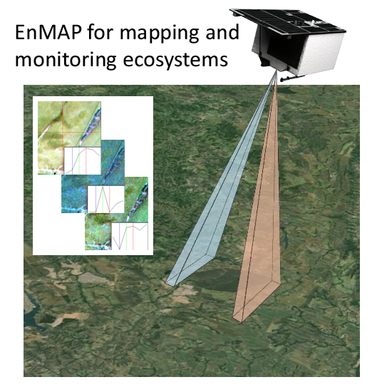
Monitoring Natural Ecosystem and Ecological Gradients: Perspectives with EnMAP

by
Pedro J. Leitão
1,*,
Marcel Schwieder
1,
Stefan Suess
1,
Akpona Okujeni
1,
Lênio Soares Galvão
2,
Sebastian Van der Linden
1 and
Patrick Hostert
1
1
Geography Department, Humboldt-Universität zu Berlin, Unter den Linden 6, D-10099 Berlin, Germany
2
Divisão de Sensoriamento Remoto, Instituto Nacional de Pesquisas Espaciais (INPE), Avenida dos Astronautas, 1758, Bairro Jardim da Granja, Caixa Postal 515, São José dos Campos, SP 12227-010, Brazil
*
Author to whom correspondence should be addressed.
Remote Sens. 2015, 7(10), 13098-13119; https://doi.org/10.3390/rs71013098
Submission received: 1 June 2015 / Revised: 15 September 2015 / Accepted: 29 September 2015 / Published: 2 October 2015

Abstract

:
In times of global environmental change, the sustainability of human–environment systems is only possible through a better understanding of ecosystem processes. An assessment of anthropogenic environmental impacts depends upon monitoring natural ecosystems. These systems are intrinsically complex and dynamic, and are characterized by ecological gradients. Remote sensing data repeatedly collected in a systematic manner are suitable for describing such gradual changes over time and landscape gradients, e.g., through information on the vegetation’s phenology. Specifically, imaging spectroscopy is capable of describing ecosystem processes, such as primary productivity or leaf water content of vegetation. Future spaceborne imaging spectroscopy missions like the Environmental Mapping and Analysis Program (EnMAP) will repeatedly acquire high-quality data of the Earth’s surface, and will thus be extremely useful for describing natural ecosystems and the services they provide. In this conceptual paper, we present some of the preparatory research of the EnMAP Scientific Advisory Group (EnSAG) on natural ecosystems and ecosystem transitions. Through two case studies we illustrate the usage of spectral indices derived from multi-date imaging spectroscopy data at EnMAP scale, for mapping vegetation gradients. We thus demonstrate the benefit of future EnMAP data for monitoring ecological gradients and natural ecosystems.

Graphical Abstract

1. Introduction

Global environmental change is occurring at unprecedented rates, resulting in a sharp decrease in pristine ecosystems globally [1,2]. This urges systematic monitoring of the Earth’s surface, and particularly of natural or quasi-natural areas from local to global scales. Only through monitoring and analysis of ecosystem processes it is possible to deepen our understanding of anthropogenic global environmental impacts, e.g., by feeding information into complex ecosystem models [3].
Natural ecosystems, unlike managed ones, are intrinsically heterogeneous and dynamic, formed of vegetation continua and ecological gradients [4,5]. With gradients we refer to gradual changes or transitions, both in time and in space [6], of ecosystem characteristics, be it biotic or abiotic. Spatial gradients result from the spatial patterns of ecosystems and living communities, which include large-scale geographical and climatic (e.g., latitudinal and altitudinal) variability [7], as well as small-scale spatial variation in the respective system’s biogeochemical cycle [8]. Temporal gradients refer to the change in ecosystems or their conditions from one point in time to the next. This can include short-term, seasonal or phenological changes within a year-time [9], or longer-term changes such as e.g., changing ecosystems as a result from changing climatic conditions [10]. Ecological gradients can also be the direct outcome of human disturbances to the system. Most typical gradients of anthropogenic origin include spatial or temporal rural-to-urban transitions (Figure 1) [11], shrub encroachment following agricultural land abandonment [12], forest degradation [13], overgrazing [14] or exotic species invasions [15]. Indeed, successional shrub encroachment following agricultural land abandonment, or vegetation regeneration at the deforestation frontier constitute typical examples of spatio-temporal gradients. Both typically show a landscape (spatial) gradient of patches at different stages of vegetation regeneration and re-growth, in itself a gradual process in time [16,17]. Additionally, ecological gradients largely determine the patterns and composition of biotic communities with direct implications on ecosystem functioning and the provided services [18,19,20], thus highlighting the importance of monitoring ecosystem transitions.
Quantifying ecosystem characteristics, however, requires using information at the meso- to macro-scale, which needs to be consistent and reproducible through space and time. Remotely sensed data of the Earth´s surface is thus the ideal source of such information [21,22]. On the temporal domain, time-series of remotely sensed data allow ecosystem monitoring based on climate or disturbance related vegetation changes and their phenological patterns [23,24]. Moreover, the recent opening of the Landsat archive has made available a valuable dataset, which enables a detailed characterization of dynamic ecosystem processes at landscape scales, such as e.g., disturbances or long-term trends [25]. This has been followed by a wealth of studies recurring to this archive for ecosystem change monitoring [26,27].
Figure 1. Gradient of vegetation cover fractions along a rural-to-urban transect in Berlin captured by simulated Environmental Mapping and Analysis (EnMAP) data (white line): (Top) false-color simulated EnMAP data (Red-Green-Blue: 833, 1652, and 632 nm). (Bottom) Different mean (across track) vegetation cover fractions along the transect (for further details on the vegetation fraction mapping see [28]).
Remotesensing 07 13098 g001
Imaging spectroscopy (IS) data, i.e., data with a high number of contiguous and narrow spectral bands, allow a precise characterization and quantification of relevant ecosystem properties, such as vegetation physiognomies or plant functional types [29,30]. Numerous studies made use of field-based or airborne spectral measurements for quantifying biophysical parameters related to the natural vegetation, such as primary production, leaf area index or photosynthetic activity [31,32], biomass [33], carbon storage and water fluxes [34], ecosystem structure [35], species turnover [36,37], or vegetation successional stage [38]. These highly detailed data have also been used for monitoring anthropogenic ecosystem disturbances, such as overgrazing [39] or species invasions [40].
Most of these studies, however, were limited to few acquisitions (one per year or less), and none of those studies could use high quality, landscape scale IS data, as the Environmental Mapping and Analysis (EnMAP) mission will provide [41]. Few studies have so far used simulated EnMAP data [42] to monitor gradual ecosystem changes [28,37,43]. The high temporal and systematic coverage of the EnMAP system will allow for continuous monitoring and the study of ecosystem processes and properties [44], as demonstrated by some pilot studies using data from experimental spaceborne systems [45,46]. Currently, the only spaceborne full width IS sensor in orbit is the Hyperion onboard the Earth Observing One (EO-1) platform, which delivers a low Signal to Noise Ratio (SNR), particularly in the shortwave infrared (SWIR) spectral region. Despite these limitations, a few studies have made use of time series of Hyperion data for ecosystem monitoring, covering topics like seasonal vegetation dynamics [47,48] and invasive species mapping [49,50]. These studies show that repeatedly acquired high spectral resolution data are likely to reveal new insights on vegetation condition, change and phenology, thus improving existing carbon emission accounts and monitoring efforts effective [51]. Such findings, which would have not been possible to achieve solely based on multispectral imagery, are of fundamental relevance to global change mitigation programs such as the Reducing Emissions from Deforestation and forest Degradation (REDD), REDD+ or the Convention on Biological Diversity [52]. These studies hence highlight the importance of hyperspectral satellite sensors, which can assure multiple and systematic acquisitions of highly detailed data suitable for monitoring ecosystem dynamics.
In this paper, we present some of the preparatory research activities of the EnMAP Scientific Advisory Group (EnSAG) on natural ecosystems and ecosystem transitions (EnSAG-Ecosystems), alongside the work previously published [37,43] and that published in the current issue [53]. Our aim is to demonstrate the benefit from high quality spaceborne IS data, like EnMAP, for characterizing and quantifying gradual ecosystem transitions and natural ecosystems. We also include two illustrative case studies using IS data at the EnMAP scale to describe gradients of vegetation: one in Southern Portugal and another in Central Brazil.

2. Monitoring Ecological Gradients with Spaceborne IS Data

While physically-based modeling of natural vegetation is in many cases unfeasible due to its complexity and heterogeneity, advances in statistical and machine learning (e.g., Support Vector Machines or Random Forests) provide great opportunities for analyzing complex data problems [54,55] with clear advantages over traditional methods, e.g., when dealing with high-collinear datasets [56]. Indeed, spaceborne IS data collected over heterogeneous landscapes and covering ecological gradients are characterized by high complexity and gradually changing mixtures (fractions) of diverse surface covers. Utilizing machine learners thus bears great potential for adequate information extraction of highly detailed and complex data such as the forthcoming EnMAP data for ecosystem analysis and monitoring [37,57]. Additionally, these methods allow the combination of empirical relations between specific spectral regions (e.g., in the form of spectral indices) and biophysical parameters.
IS data also create challenges for analysis and transferability of modeled relationships, as, e.g., spectral autocorrelation in high-dimensional feature space hampers straightforward information extraction. Feature reduction or extraction becomes important, e.g., in-built in machine learning algorithms [58] or based on statistical redundancy [59]. Nevertheless, the use of narrow-band spectral indices have been shown very useful for quantifying vegetation foliar and canopy chemistry patterns [60,61,62], thus constituting a great potential for dealing with data redundancy. In addition, as they directly describe ecosystem properties, they can be considered proximal predictors. While modeling with such type of predictors ensures model transferability [63], the combined use of advanced machine learning algorithms, further allows maximal information extraction.
In the following, we present two case studies using spectral indices derived from IS data at the EnMAP scale to analyze vegetation cover gradients. One refers to a gradual ecosystem transition (from grassland to shrublands) in a study site in Southern Portugal that faces successional shrub encroachment. The second case study builds upon work-in-progress in the Brazilian Cerrado, a spatio-spectrally complex savanna ecosystem. While the usage of narrow-band spectral indices does not cover all possibilities of use of the future EnMAP data for ecosystem research, it does however illustrate one potential research avenue to be considered.

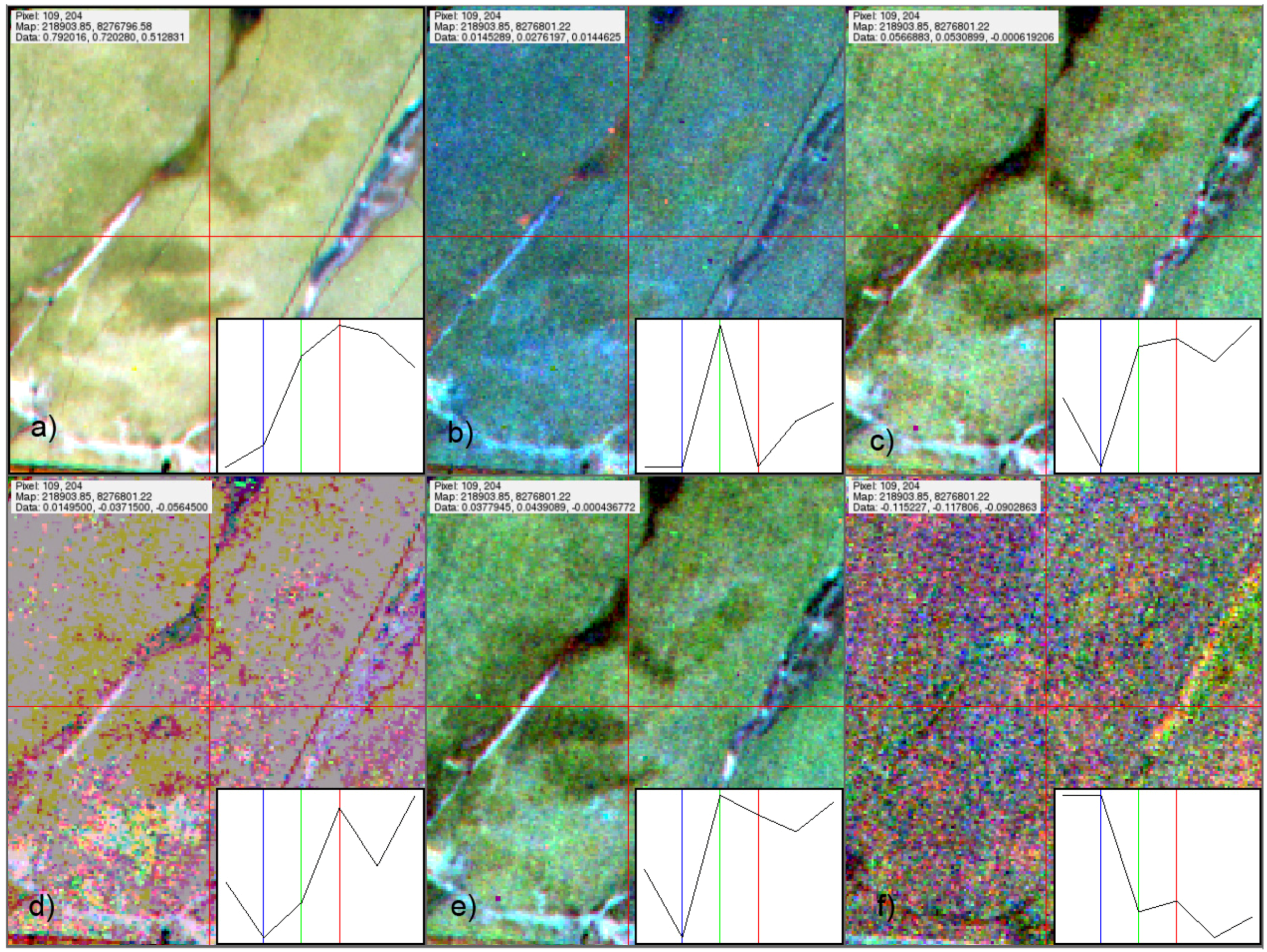
2.1. Common Methodological Approach

Both cases make use of multi-date narrow-band spectral indices, this way coupling the spectral and temporal information domains. To this effect, we used six indices (Table 1), which relate to different biophysical and physiological properties of the surface’s vegetation, such as chlorophyll, water or lignin content. Information on these properties and their development along the phenological cycle should allow a detailed characterization of the vegetation condition and cover, at the sub-pixel level (fractions). All spectral indices were calculated in the EnMAP-Box [64].
Table 1. Narrow band spectral indices used in the analysis, usage and spectral bands used
NameUsageSpectral Bands (nm)Reference
Normalized Difference Vegetation Index (NDVI)Structure, vigor670, 800[60]
Modified Chlorophyll Absorption in Reflectance Index (MCARI)Chlorophyll550, 670, 700[65]
Leaf Water Vegetation Index (LWVI2)Leaf water1094, 1205[66]
Cellulose Absorption Index (CAI)Cellulose2000, 2100, 2200[67]
Normalized Difference Lignin Index (NDLI)Lignin1680, 1754[61]
Normalized Difference Nitrogen Index (NDNI)Nitrogen1510, 1680[61]
Both case studies aim at estimating vegetation cover fractions by fitting either subsets or the full spectral index time series data, as described below. The data analysis was done using Boosted Regression Trees (BRT), a machine learning approach that combines the strengths of decision trees and boosting [68]. Decision trees analyze the variation of a response variable for a set of predictor variables, which are then subject to subsequent binary splits that fits simple models to each resulting section until achieving the best model split [68]. BRT is based on an ensemble approach, which fits multiple decision trees to the data, in order to optimize the predictive performance of the final model. BRT are highly performing as they incorporate stochasticity in the models, using only a random subset from the data to fit each tree, and its sequential (stage-wise) model fitting, meaning that each new tree builds on previously fitted trees [68]. Furthermore, this approach allows for prediction, the inspection of individual variable responses (through partial dependency plots), and ranking of predictor variable importance, and has thus been widely used in various research domains [69,70,71]. This approach should thus allow maximal information extraction from the spectral indices.
The reference data were fit to the spectral indices using BRT, which was done in R [72] using modified code from the “gbm” package [68,73]. In this implementation, the BRT parameterization requires the input of two parameters, one relating to the level of shrinkage, i.e., the contribution of each tree to the growing model, and the other to the maximum level of interactions, i.e., the tree complexity or tree depth. These two parameters then define the number of trees to be fitted for optimal prediction [68]. We did this through a heuristic grid search based on a five-fold cross-validation, to optimize for withheld variance explained (coefficient of determination r2). The best parameter pair was selected and the subsequent models were reduced by eliminating the least explanatory variables in a back selection manner [68]. The models were validated by a 10-fold cross-validation using the r2 measure—in the current implementation of BRT, the only performance measure available for models with Gaussian-like response variables. All models were re-iterated 21 times, which allows the inference of statistical significance (p < 0.05) of the model performances and the importance of the input variables. The mean (out of all iterations) model performances, and importance of the significant variables were thus calculated. Finally, the differences in model performances between different models were also tested for their significance.
It is expected that adding temporal information to that provided by the spectral indices, by describing changes in biophysical conditions of vegetation throughout the phenological cycle, improves its characterization. It is also expected that the usefulness of the different spectral indices (describing different biophysical conditions of the vegetation) for characterizing the vegetation cover varies throughout the phenological cycle. In order to test the tradeoffs between the temporal and spectral data domains, we ran (multi-index) models (fitting all six spectral indices) for each available data acquisition (single-date) and for the time-stack (multi-date), on both case studies. Additionally (for the second case study only), we ran single-index models fitting the temporal profiles (i.e., all acquisitions) of each individual spectral index at a time. The model results were finally compared in terms of their performances and of the importance of the variables selected by the models.

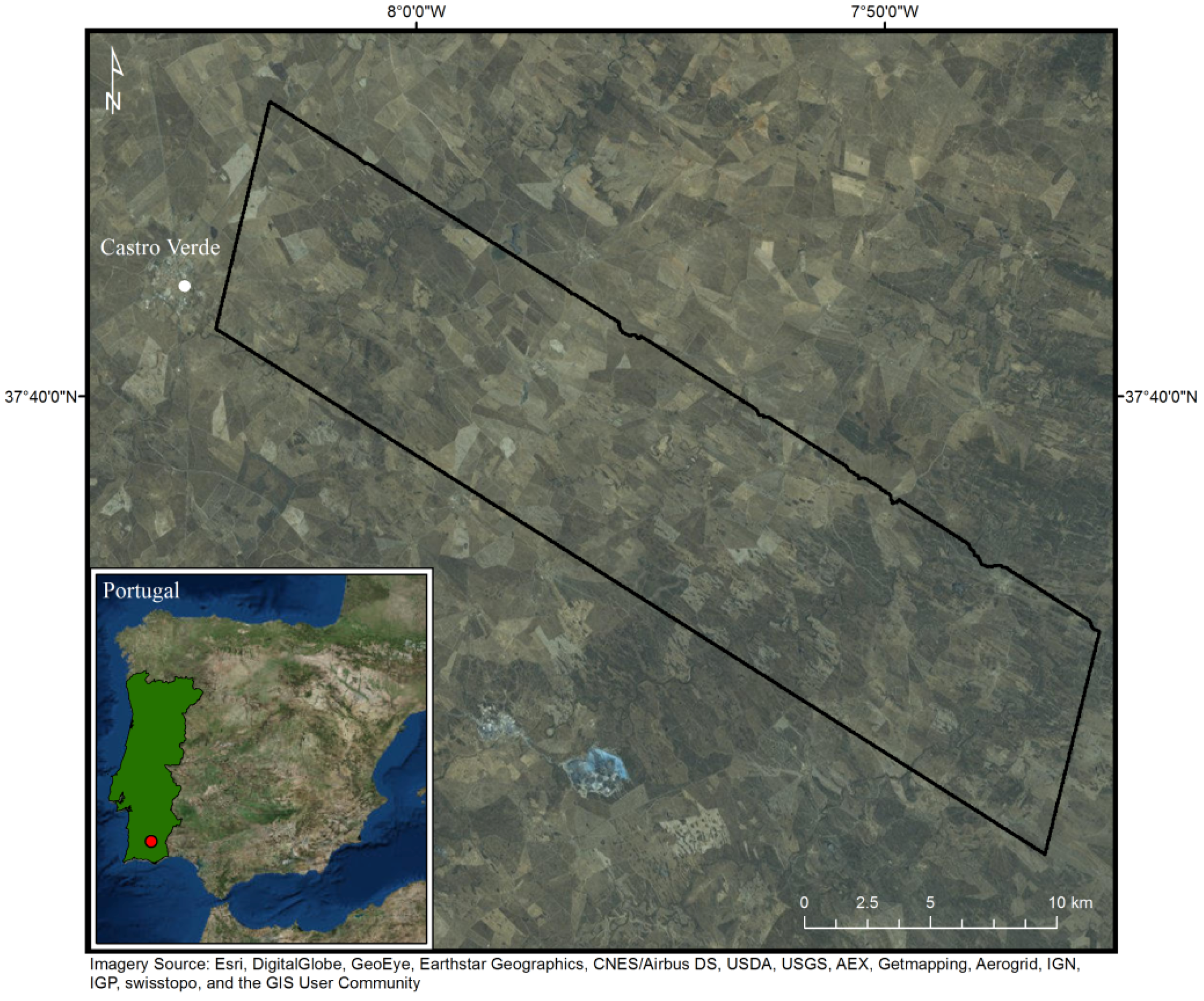
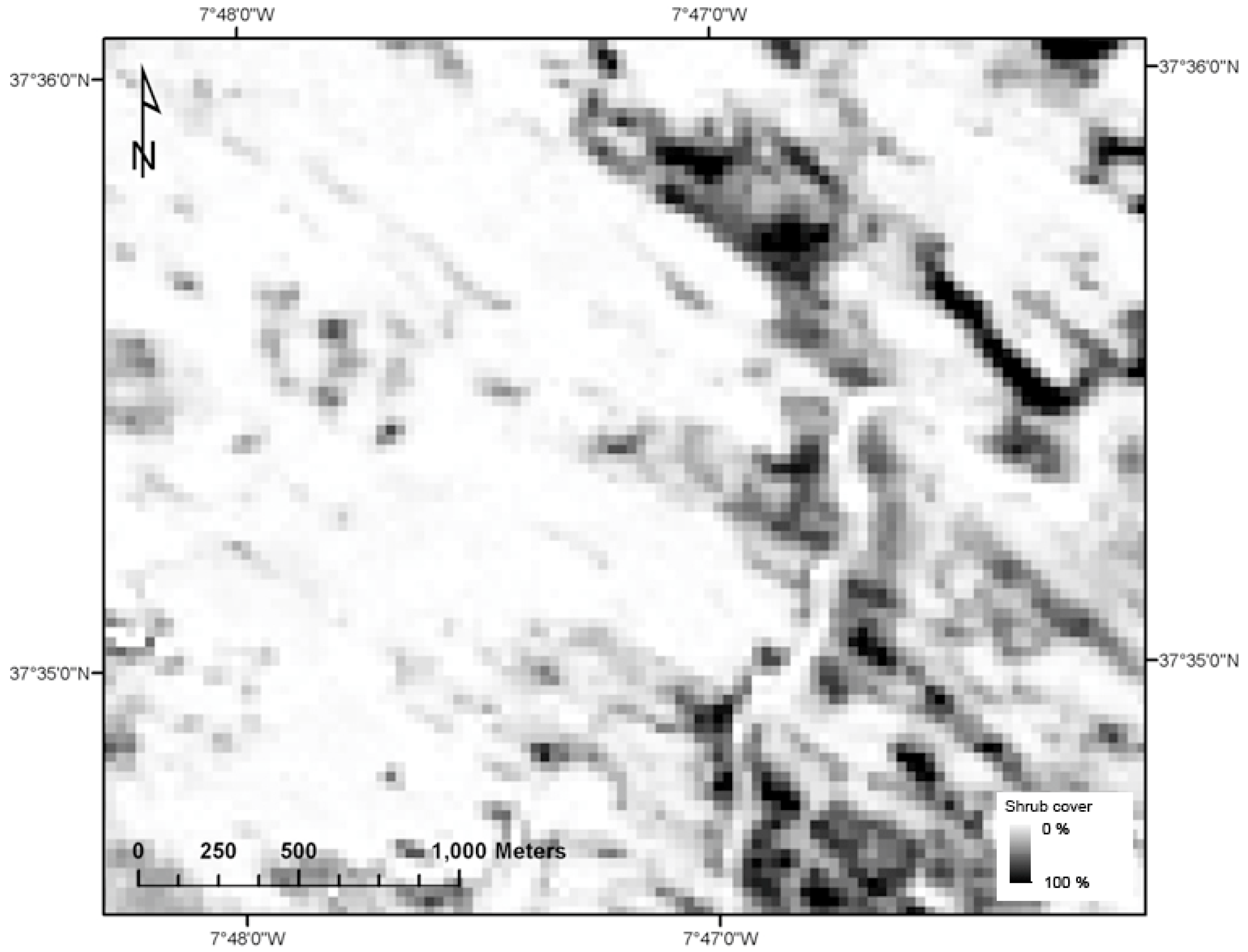
2.2. Gradual Ecosystem Transitions: Shrub Encroachment in Southern Portugal

The cultural landscapes of Southern Portugal (Figure 2), known as pseudo-steppes, are characterized by very extensive agriculture, largely dominated by grazed fallow grasslands and scattered winter cereals on a rotation basis [74]. The NW part of the study area is within a designated Special Protection Area (SPA) for birds, holding internationally important populations of several steppe bird species, and is subject to a specific agri-environment scheme [75]. This scheme is based on subsidy payment to farmers to maintain traditional agricultural practices, this way conserving the pseudo-steppe landscape and promoting its local biodiversity. Outside the SPA, the region’s poor and skeletal soils and the lack of land use incentives, lead to widespread land abandonment and subsequent successional shrub encroachment [43]. This is a typical case of an ecosystem transition (spatio-temporal gradient), observed in other parts of the world, as e.g., in Eastern Europe after the fall of the Socialist regimes [76]. While the successional encroachment of shrubby and woody vegetation has deep implications on ecosystem functioning [12], the study region presents a management challenge with conflicting interests between biodiversity and soil conservation [77]. Monitoring this ecological gradient is therefore of major relevance towards the sustainable management of these landscapes.
We thus aim at modeling the fractional shrub cover along the shrub cover gradient in the region, by recurring to multi-date EnMAP-like data. In this case study, we used simulated EnMAP data corrected to surface reflectance [42], which was derived from the Airborne Imaging Spectrometer for Applications (AISA) Eagle and Hawk data at a ground sampling distance (g.s.d.) of 5.4 m, acquired (from an altitude of 4500 m) in two airborne campaigns in April (7 April 2011) and August 2011 (11 August 2011) over the study region [43]. From these data, the described spectral indices (Table 1) were calculated for use in the analyses.
Figure 2. Study area in the Castro Verde region in Southern Portugal, characterized by agricultural land abandonment (NW–SE gradient) leading to successional shrub encroachment.
Remotesensing 07 13098 g002
As reference data, we used an independent high spatial resolution (g.s.d. of 1.8 m) land cover map (overall accuracy of 94.2%), derived from AISA Eagle and Hawk imagery acquired from an altitude of 1500 m obtained during the abovementioned air campaigns. This land cover map was resampled to the EnMAP pixel size to calculate the respective shrub cover fractions [43], used as the response variable in the models.
Both predictors and response variables were thus calculated from these datasets. For the analysis we sorted 80 sample points in a stratified random manner, which can be considered a realistic (field collected) sample size.
BRT models were used to fit the spectral index values on the shrub cover fractions (multi-index models), for each of the single time-steps (April and August), and for the time-stack. The single-index models, based on the temporal profiles of each spectral index, were skipped in this case study, as the time-stack and respective profiles are constituted of just two acquisitions.
The April models were the weakest, with a mean predictive performance of only ca. 0.16 (Table 2). The background (herbaceous) vegetation is highly heterogeneous at this time of year (spring greening peak), with various degrees of cover from photosynthetically active vegetation, possibly dominating the pixel’s reflectance. In August, the annual (herbaceous) vegetation is dry and the contrast between shrub and background is highest. This period of the year is therefore considered the best time for discriminating shrubby vegetation from the background [78]. These models delivered a mean predictive performance of ca. 0.33, which is significantly different to that of the April models. Our results, however, show a significant increase in model performance when using the time-stack (close to the sum of the performances of both single-date models), so that we can conclude that the temporal (phenological) information was an added value to the models.
Table 2. Mean model performances (r2) and variable importance (%) in the respective Boosted Regression Trees (BRT) models. Variables not significantly selected by the models have no importance reported.
AprilAugustTime-Stack
NDVI23%61%46% (August)
MCARI24%13% (April)
LWVI224%19% (August)
CAI19%
NDLI34%18% (April)
NDNI
r20.1590.3310.446
The models fitted on the April data had a greater contribution (34%) of the lignin index (NDLI), followed by those relating to chlorophyll (MCARI) or vegetation vigor (NDVI)—with respective levels of importance of 24% and 23%. This makes sense, as during this period the background herbaceous vegetation dominates the signal of MCARI and NDVI indices. Of least importance (19%), though significantly selected by the models was the cellulose absorption index (CAI). Indices related to leaf water or nitrogen contents were not significantly selected in the models. In the models based on the August data, on the other hand, the NDVI showed to be the most relevant index to model fractional shrub cover (with an importance of 61%). This is not surprising as the herbaceous vegetation is dry in August and shrub cover alone provides the spectral signature in the visible red and near infrared wavelengths regions. The index related to leaf water content (LWVI2) was weighted second importance (24%), and none of the remaining indices were significantly included in the models. In the time-stack models, the most contributing variable (46%) was the NDVI from August, followed by the water content (August) and lignin (April) indices. Of least importance (13%), although significantly selected in the time-stack models, was the chlorophyll index for April. All other indices were not significantly selected by the models.
This case study served to illustrate the added value of IS data for modeling and mapping vegetation cover along a spatial gradient of shrub encroachment (see Figure 3), as several of the indices selected (like the LWVI2 or the NDLI) by the models require spectral regions that are not covered by the most common multi-spectral sensors. The availability of multi-date imagery further improved the models, thus highlighting the importance of repeated IS data acquisitions, such as coming from a spaceborne platform like the future EnMAP. The results from such a study allows the assessment of system’s condition. The systematic mapping of these landscapes using a comparable approach (e.g., by transferring a model to a new set of imagery data), would allow measuring the gradual changes (temporal gradients) of shrub cover, and this way monitor the development of the encroachment process. This would provide the necessary knowledge for adopting adequate management options towards the sustainability of the system.
Figure 3. Spatial gradients of shrub cover, as derived from the land cover map of the study area resampled to a ground sample distance (g.s.d.) of 30 m (adapted from [43]). In this image, brighter pixels correspond to areas with low shrub cover, and darker ones correspond to areas with higher (successional) shrub cover. The gradual transitions from bright to dark pixels illustrate the described vegetation gradients.
Remotesensing 07 13098 g003

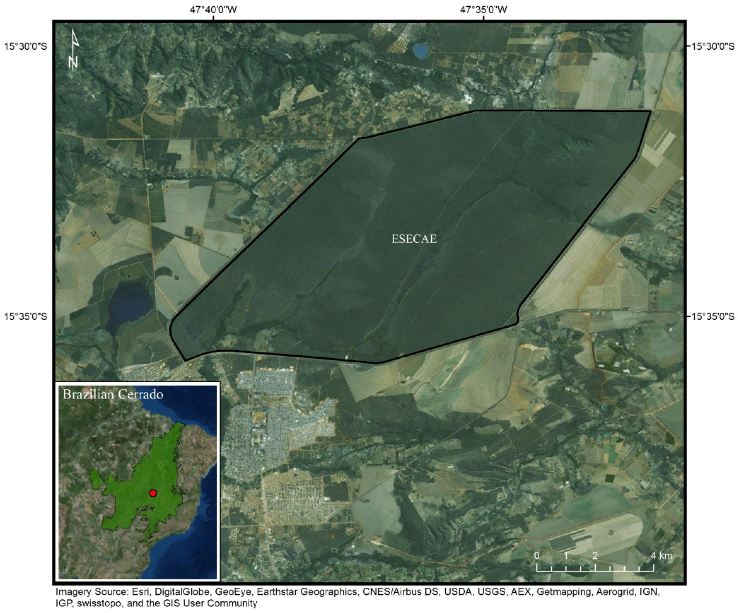
2.3. Brazilian Cerrado

The Brazilian Cerrado covers ca. 20% of Brazil’s surface and it holds the richest biodiversity of all of the world’s savannas, thus constituting one of the global biodiversity hotspots [79,80]. This system, however, is mostly unprotected and highly threatened, with an estimated conversion rate of over 40%, resulting in considerable biodiversity loss and carbon emissions [81,82,83]. The need for monitoring the Cerrado system is obvious to better understand its dynamics and thus support its sustainable management [84]. The Cerrado exhibits high climatic, edaphic and structural gradients [85,86,87], resulting in heterogeneous patterns of vegetation structure and density, which poses numerous challenges to remote sensing analyses. The Cerrado constitutes a major focus of our current research within the EnSAG-Ecosystems activities, where we focus on modeling and mapping the different Cerrado vegetation physiognomies [88], Cerrado vegetation cover, and ultimately its aboveground biomass and plant community transitions [37].
The current case study, although still preliminary, aims at modeling the vegetation cover, which intrinsically relate to vegetation biomass and respective carbon storage potential of these landscapes. The study is conducted in a region within the Estação Ecológica de Águas Emendadas (ESECAE), in the Brazilian Federal District, where most Cerrado vegetation physiognomies are present (Figure 4).
Figure 4. Study area in the Brazilian Cerrado: Estação Ecológica de Águas Emendadas (ESECAE).
Remotesensing 07 13098 g004
Here we referred to a six-step time series of EO-1 Hyperion data (acquired between August 2006 and May 2007) for analysis, which cover most of the yearly phenological cycle (Table 3). These data allow us to infer on the value of future EnMAP data, as both sensors (Hyperion and EnMAP) share the same spatial resolution (g.s.d. of 30 m), although Hyperion’s low SNR will be clearly outperformed by EnMAP [41]—most particularly in the SWIR region, with a reported SNR of 180:1 at 2200 nm, instead of 40:1 for Hyperion at similar wavelengths. The data were pre-processed (radiometric atmospheric and geometric corrections), including the correction of known problems of data striping, pixel shift, keystone and spectral smiling, resulting in surface ready-to-use reflectance data [89].
This time series was the base for calculating the six narrow-band spectral indices (Table 1) for each time-step. This also allowed us to build temporal profiles for each spectral index for the use in the (multi-date) single-index models (Figure 5).
Table 3. EO-1 Hyperion data acquisitions over the study area.
DateView Angle (°)Season
2006-08-296.25Dry season
2006-09-1313.12End of dry season
2006-11-19−5.77Beginning of wet season
2007-02-1017.51Wet season
2007-03-022.20Wet season
2007-05-176.70End of wet season
Figure 5. Screenshot of the temporal profiles of the six spectral indices plotted in RGB (Red-Green-Blue: 2007-02-10; 2006-11-19; 2006-09-13), with central pixel profiles displayed in the respective lower right corner: (a) NDVI; (b) MCARI; (c) LWVI2; (d) CAI; (e) NDLI; and (f) NDNI, as visualized in the EnMAP-Box [64]. Particularly in the CAI and NDNI plots, it is possible to observe high level of noise in the data (due to the low SNR of Hyperion).
Remotesensing 07 13098 g005
Due to the lack of field-based data, we derived the reference data directly from image data. For this purpose we used the panchromatic band of the Advanced Land Imager (ALI) sensor, which is (alike Hyperion) onboard of the EO-1 platform and captures the surface’s albedo at a high spatial resolution (g.s.d. 10m). At the end of the dry season (August image), the contrast between the dark woody (perennial) vegetation and the light background (soil and yearly herbaceous vegetation) is at its highest [90], which makes the surface’s albedo a good proxy for (woody) vegetation cover. We have thus resampled the ALI panchromatic data to the Hyperion g.s.d. to serve as a measure of vegetation cover for the use as response variable in the conducted analyses (Figure 6).
Both predictors and response variables were calculated from these datasets. In this case study, due to its higher complexity (full vegetation gradient from grassland to woodland), we sorted 150 sample points in a stratified random manner, equivalent to a higher field sampling effort (when compared to the previous case study).
BRT models were used to fit the spectral index values to the vegetation cover (multi-index models), for each of the single time-steps, and for the full time-stack. The dry season acquisition (August), however, was excluded from the analyses due to its high dependency with the reference data—both data were acquired simultaneously from the same platform (EO-1), so they share, e.g., the same view angle bias effects. Single-index models, based on the temporal profiles of each spectral index, were also performed in this case study.
Figure 6. Spatial gradients of Cerrado vegetation cover, as captured by the panchromatic band of the Earth Observing One (EO-1) Advanced Land Imager (ALI) sensor (resampled to a g.s.d. of 30 m). In this image, brighter pixels correspond to low vegetated areas (bare soil and grasslands) where darker ones correspond to more densely vegetated areas (dense savannah woodlands and riparian galleries). The gradual transitions from bright to dark pixels illustrate the described vegetation gradients.
Remotesensing 07 13098 g006
Our results showed that the best performing models were the ones based on the (multi-index) time-stack (with a cross-validated r2 of 0.681), on the (multi-index) September data (0.688) and on the (single-index) NDVI temporal profiles (0.680), with no significant differences between them. Indeed, all of these models included only one (and the same) significant variable, namely the NDVI for the September acquisition—this variable alone contributed with 85%, 96% and 94% to the respective models.
Within the multi-index models (Table 4), those based on the November and May data followed in performance (respective mean r2 of 0.608 and 0.590, non-significantly different). The March models had a mean predictive performance of 0.492, and the weakest models were those using the February data with a mean r2 of 0.392. While the NDVI was always the most important (and significant) variable on all models, the leaf water content index was also significantly selected in the November, February and the May models, with a variable importance up to 34% (in the February models). Additionally, the cellulose absorption index was significantly selected by the March models.
The single-index models (Table 5) that followed in performance were those based on the leaf water (r2 of 0.581) and lignin (0.572) indices, non-significantly different. The models based on the chlorophyll absorption followed (with a mean performance of 0.539), and then those based on the cellulose index (0.477). Finally, the models based on the nitrogen content were the weakest, with a mean performance of only 0.097. In these models, the data from the nearest date to that of the reference data (September) were always significantly selected, being this the most important model variable in the NDVI (94%), MCARI (81%) and NDNI (60%) models. On the other hand, data from November were also significantly used in the MCARI, LWVI2 and NDLI models, being the most important variable in the two latter ones (respective importance of 77% and 79%). The CAI based model had the data from March as the most important (50%), followed by September (25%) and May (22%).
Table 4. Mean performances of the multi-index models (r2) and importance of the spectral indices, according to their contributions in the BRT models. Variables not significantly selected by the models have no importance reported.
SeptemberNovemberFebruaryMarchMayTime-Stack
NDVI96%33%57%70%77%85% (September)
MCARI
LWVI228%34%19%
CAI20%
NDLI
NDNI
r20.6880.6080.3920.4920.5900.681
Table 5. Mean performances of the single-index models (r2) and ranking of acquisition dates, according to their contributions in the BRT models. Variables not significantly selected by the models have no importance reported.
NDVIMCARILWVI2CAINDLINDNI
September94%81%18%25%16%60%
November19%77%79%
February39%
March50%
May22%
r20.6800.5390.5810.4770.5720.097
In this case study, we illustrated the usefulness of multi-date IS data for modeling (spatial) gradients of vegetation cover, while testing the tradeoffs between the spectral and temporal domains of information. When dealing with ecological gradients, the Cerrado is possibly the ideal system to study, as it is constituted by the combination of several different spatial gradients (as previously described), which result in a complex mosaic of different vegetation physiognomies. It is also a highly dynamic system, including a high frequency of fire occurrence and resulting vegetation successional dynamics. Only through the usage of replicable and transferable methods, such as the ones presented, it is possible to assess this complex system. Indeed, the monitoring of this globally important yet threatened ecosystem requires the systematic quantification and mapping of the spatial and temporal gradients of ecosystem properties such as vegetation cover, biomass or carbon stored.

3. Discussion

Our case studies demonstrated that spaceborne IS data collected at repeated times have the potential to monitor gradual ecosystem transitions as well as heterogeneous landscapes. While the use of narrow-band spectral indices could relate to specific vegetations properties, their development through time could depict changes in vegetation conditions along the phenological cycle. This had also been demonstrated in a study in the Cerrado, which made use of spectral indices derived from MODIS to describe annual vegetation dynamics [90]. Indeed, we observed that while the narrow-band NDVI was determinant in explaining the variance in most models, the leaf water content index (LWVI2) was also highly contributing in models fit on the EnMAP simulated data and in most multi-index models fit on (single-date) Hyperion data. This finding is particularly relevant, as this narrow-band spectral index uses a spectral region not available in multispectral sensors. We also found that the several spectral indices contributed differently in the models depending on the respective stage of the vegetation’s phenological cycle. For example, in the first case study the lignin index (NDLI) was the second most contributing variable when fitting the shrub fractional cover to the August EnMAP simulated data, whereas it was the third in the time-stack models, being LWVI2, respectively, the second most contributing variable. This emphasizes that both spectral and temporal data domains contribute with complementary information for describing such complex systems. The potential usage of narrow-band spectral indices as an expert-based feature reduction method for IS data was also demonstrated in the first case study. Indeed, making use of six spectral indices, effectively using information from 13 spectral bands, we achieved good results. On the other hand, similar studies covering the same study region, which made use of the full EnMAP simulated spectra achieved better results [43,53]. Indeed, not all important spectral features from these studies were covered by the six spectral indices here used, thus suggesting the potential relevance of further research, e.g., in identifying important (and robust) spectral regions (or indices) for the characterization of specific ecosystem properties.
Our second case study has more limitations, particularly in what relates with the reference data. On the one side, the reference data was derived from an image and has therefore no direct translation into field measures. On the other side, it was derived from data collected by a sensor onboard the same platform (the EO-1 satellite), therefore sharing data bias resulting from the acquisition of orbital imagery, such as local atmospheric effects or view angle effects. For this reason, and as we used ALI data collected at the peak of the dry season for the extraction of the reference data (August), we could not use Hyperion data from this date for modeling (to ensure a certain level of reference data independency). This is clearly a limitation as the dry season is the considered to be the best period to discriminate the different Cerrado vegetation physiognomies [91]. Indeed, the respective model results were also more limited. For example, the fact that all three best performing models (multi-index September and time stack, and single-index NDVI models) only significantly used the NDVI variable from a single acquisition date (September), does not allow us to draw any conclusions relating to the usage of multi-date IS data for ecosystem monitoring. In fact, the temporal phenological gradient of the Cerrado vegetation probably results in a high temporal dependence of this variable and the reference data, as both images were acquired only 15 days from each other (29 August 2006 and 13 September 2006). On the other hand, the significant selection of, e.g., the leaf water and cellulose indices in several of the multi-index models, which use spectral regions not covered by multi-spectral systems, highlight the usefulness of IS data for ecosystem modeling. In addition, the relatively good results of some of the single-index models, further highlight the value of time series of spaceborne IS data for monitoring ecosystem parameters in complex landscapes.
We have thus demonstrated that time series of spaceborne IS data, by linking both the spectral and the temporal domains of information, are suitable for characterizing ecosystem processes and patterns, such as ecological gradients or complex (heterogeneous) landscapes. Our tests on Hyperion data were also successful in demonstrating this. While data coming from the Hyperion sensor is known to be noisy, and most particularly in the SWIR spectral region (see, e.g., Figure 4d,f), we found that most indices used were able to deliver reasonable results, with the exception of the nitrogen index (with spectral bands on the 1510 and 1680 nm). For example, while the CAI index showed erroneous values at random pixel locations, the BRT models were still able to extract useful information from the temporal profiles. This further demonstrates the strengths of machine learning algorithms in dealing with complex (and noisy) data problems [56,68].
The Hyperion sensor, though with its limitations relating to data quality, by being the only spaceborne full width IS sensor available, showed to be essential for demonstrating the benefits of usage of these types of data for ecosystem monitoring. Data coming from the forthcoming EnMAP sensor, on the other hand, with highly increased data quality (much higher SNR values on all spectral regions), and with much larger image swath (30 km instead of 7.5 km), will allow for a better description of natural ecosystem processes, with much higher precision than ever before. It is thus important to develop robust models, capable of being transferred to larger or other regions (e.g., through the use of proximal predictors, such as spectral indices), to take the most benefit of these improved properties of the EnMAP sensor for ecosystem monitoring.
Furthermore, it is expected that the synergies between the spectral and temporal information from multiple acquisitions of EnMAP data will be crucial in describing ecosystem gradients of higher complexity. As such, ongoing research within our activities focus on mapping vegetation communities, aboveground biomass and carbon storage in the Cerrado, as a demonstration of the usage of EnMAP data for natural (complex) ecosystem monitoring in a detailed manner [41].
The usage of narrow-band spectral indices clearly does not exhaust the full potential of the future EnMAP data for ecosystem monitoring, but rather illustrates one possible research avenue. Indeed, continued work within the EnSAG-Ecosystems activities has been making use of several statistical and machine learning methods for inferring different ecosystem properties from EnMAP-like data [37,43,53]. Nevertheless, further research is still necessary for a full assessment of the value of EnMAP for ecosystem research. Particularly the analysis of trade-off and synergies between real EnMAP data, once available, and those from other platforms, such as airborne IS or spaceborne multispectral systems (e.g., Landsat OLI or the Sentinel’s). Finally, the continuous work of the EnSAG further contributes to the development of methods and algorithms for handling such complex data [41].

4. Conclusions

We conclude that EnMAP data will be extremely useful for mapping and monitoring natural ecosystems and their services, by allowing the detailed characterization of complex and heterogeneous landscapes. Indeed, its high spectral resolution with much improved SNR, allied to its wide spatial coverage and frequent revisit period will guarantee a highly detailed spectral, spatial and temporal coverage of the Earth’s surface. With EnMAP, we will be a step further towards accurately and systematically mapping and quantifying gradual biophysical parameters at the sub-pixel level, such as e.g., species communities, primary production, aboveground biomass, or carbon storage potential. It will constitute a major technological development and a valuable tool for addressing urging global challenges, such as understanding current anthropogenic impacts and their effects on ecosystem dynamics. EnMAP will hence contribute to global mitigation programs, such as REDD and REDD+ or the Convention on Biological Diversity.

Acknowledgments

This study is part of the research activities of the EnMAP Scientific Advisory Group (EnSAG), and was funded by the German Aerospace Centre (DLR) — Project Management Agency, granted by the Ministry of Economics and Technology (BMWi grant 50EE1309). Data acquisition was also partly funded by the European Facility for Airborne Research (EUFAR) with the HyMedEcos-Gradients project (EUFAR 11-04) with support from the Airborne Research and Survey Facility (ARSF), Geodetic Equipment Facility (GEF) and Field Spectroscopy Facility (FSF) of the UK’s Natural Environmental Research Council (NERC). We gratefully acknowledge support by the Liga para a Proteção da Natureza (LPN) during the field campaigns in Portugal. The authors would like to thank Karl Segl and Christian Rogass from the German Research Center for Geosciences (GFZ Potsdam), for simulating the EnMAP imagery with EeteS, and preprocessing the Hyperion data. Finally, we thank five anonymous referees, whose comments contributed to the improvement of earlier versions of this manuscript.

Author Contributions

Pedro J. Leitão designed the research, collected field data, conducted the analysis and wrote the manuscript. Marcel Schwieder collected field data and processed the CV reference data. Stefan Suess collected field data and pre-processed the AISA data. All authors contributed in writing and reviewing the manuscript.

Conflicts of Interest

The authors declare no conflict of interest.

References

  1. Walther, G.R.; Post, E.; Convey, P.; Menzel, A.; Parmesan, C.; Beebee, T.J.C.; Fromentin, J.M.; Hoegh-Guldberg, O.; Bairlein, F. Ecological responses to recent climate change. Nature 2002, 416, 389–395. [Google Scholar] [CrossRef] [PubMed]
  2. Kareiva, P.; Watts, S.; McDonald, R.; Boucher, T. Domesticated nature: Shaping landscapes and ecosystems for human welfare. Science 2007, 316, 1866–1869. [Google Scholar] [CrossRef]
  3. Sitch, S.; Smith, B.; Prentice, I.C.; Arneth, A.; Bondeau, A.; Cramer, W.; Kaplan, J.O.; Levis, S.; Lucht, W.; Sykes, M.T.; et al. Evaluation of ecosystem dynamics, plant geography and terrestrial carbon cycling in the LPJ dynamic global vegetation model. Glob. Change Biol. 2003, 9, 161–185. [Google Scholar] [CrossRef]
  4. McIntosh, R.P. Continuum concept of vegetation. Bot. Rev. 1967, 33, 130–187. [Google Scholar] [CrossRef]
  5. Muller, F. Gradients in ecological systems. Ecol. Model. 1998, 108, 3–21. [Google Scholar] [CrossRef]
  6. Gosz, J.R. Gradient analysis of ecological change in time and space: Implications for forest management. Ecol. Appl. 1992, 2, 248–261. [Google Scholar] [CrossRef]
  7. Gaston, K.J. Global patterns in biodiversity. Nature 2000, 405, 220–227. [Google Scholar] [CrossRef] [PubMed]
  8. Schimel, D.S. Terrestrial ecosystems and the carbon-cycle. Glob. Change Biol. 1995, 1, 77–91. [Google Scholar] [CrossRef]
  9. Ardö, J.; Mölder, M.; El-Tahir, B.A.; Abdalla, H.; Elkhidir, M. Seasonal variation of carbon fluxes in a sparse savanna in semi arid Sudan. Carbon Balance Manag. 2008, 3, 7. [Google Scholar] [CrossRef] [PubMed]
  10. Serreze, M.C.; Walsh, J.E.; Chapin, F.S.; Osterkamp, T.; Dyurgerov, M.; Romanovsky, V.; Oechel, W.C.; Morison, J.; Zhang, T.; Barry, R.G. Observational evidence of recent change in the northern high-latitude environment. Clim. Change 2000, 46, 159–207. [Google Scholar] [CrossRef]
  11. McDonnell, M.J.; Pickett, S.T.A. Ecosystem structure and function along urban rural gradients: An unexploited opportunity for ecology. Ecology 1990, 71, 1232–1237. [Google Scholar] [CrossRef]
  12. Eldridge, D.J.; Bowker, M.A.; Maestre, F.T.; Roger, E.; Reynolds, J.F.; Whitford, W.G. Impacts of shrub encroachment on ecosystem structure and functioning: towards a global synthesis. Ecol. Lett. 2011, 14, 709–722. [Google Scholar] [CrossRef] [PubMed]
  13. Attiwill, P.M. The disturbance of forest ecosystems—The ecological basis for conservative management. For. Ecol. Manag. 1994, 63, 247–300. [Google Scholar] [CrossRef]
  14. Adler, P.B.; Raff, D.A.; Lauenroth, W.K. The effect of grazing on the spatial heterogeneity of vegetation. Oecologia 2001, 128, 465–479. [Google Scholar]
  15. Mack, R.N.; Simberloff, D.; Lonsdale, W.M.; Evans, H.; Clout, M.; Bazzaz, F.A. Biotic invasions: Causes, epidemiology, global consequences, and control. Ecol. Appl. 2000, 10, 689–710. [Google Scholar] [CrossRef]
  16. Estel, S.; Kuemmerle, T.; Alcántara, C.; Levers, C.; Prishchepov, A.; Hostert, P. Mapping farmland abandonment and recultivation across Europe using MODIS NDVI time series. Remote Sens. Environ. 2015, 163, 312–325. [Google Scholar] [CrossRef]
  17. Müller, H.; Leitão, P.J.; Hostert, P. Vegetation dynamics, carbon stocks and turnover rates in the Amazon—Upscaling local processes with remote sensing time series. In 43rd Annual Meeting of the Ecological Society of Germany, Austria and Switzerland, Potsdam, Germany, 9–13 September 2013.
  18. Hooper, D.U.; Chapin, F.S.; Ewel, J.J.; Hector, A.; Inchausti, P.; Lavorel, S.; Lawton, J.H.; Lodge, D.M.; Loreau, M.; Naeem, S.; et al. Effects of biodiversity on ecosystem functioning: A consensus of current knowledge. Ecol. Monogr. 2005, 75, 3–35. [Google Scholar] [CrossRef] [Green Version]
  19. Lavorel, S.; Grigulis, K.; Lamarque, P.; Colace, M.-P.; Garden, D.; Girel, J.; Pellet, G.; Douzet, R. Using plant functional traits to understand the landscape distribution of multiple ecosystem services. J. Ecol. 2011, 99, 135–147. [Google Scholar] [CrossRef]
  20. Sala, O.E.; Maestre, F.T. Grass-woodland transitions: determinants and consequences for ecosystem functioning and provisioning of services. J. Ecol. 2014, 102, 1357–1362. [Google Scholar] [CrossRef]
  21. Field, C.B.; Randerson, J.T.; Malmstrom, C.M. Global net primary production: Combining ecology and remote-sensing. Remote Sens. Environ. 1995, 51, 74–88. [Google Scholar] [CrossRef]
  22. De Fries, R.; Pagiola, S.; Adamowicz, W.L.; Akçakaya, H.R.; Arcenas, A.; Babu, S.; Balk, D.; Confalonieri, U.; Cramer, W.; Falconí, F.; et al. Analytical approaches for assessing ecosystem condition and human well-being. In Ecosystems and Human Well-Being: Current State and Trends; Hassan, R., Scholes, R., Ash, N., Eds.; Island Press: Washington, DC, USA, 2005; Chapter 2; pp. 37–71. [Google Scholar]
  23. Hoare, D.; Frost, P. Phenological description of natural vegetation in southern Africa using remotely-sensed vegetation data. Appl. Veg. Sci. 2004, 7, 19–28. [Google Scholar] [CrossRef]
  24. Fisher, J.I.; Mustard, J.F.; Vadeboncoeur, M.A. Green leaf phenology at Landsat resolution: Scaling from the field to the satellite. Remote Sens. Environ. 2006, 100, 265–279. [Google Scholar] [CrossRef]
  25. Kennedy, R.E.; Andrefouet, S.; Cohen, W.B.; Gomez, C.; Griffiths, P.; Hais, M.; Healey, S.P.; Helmer, E.H.; Hostert, P.; Lyons, M.B.; et al. Bringing an ecological view of change to landsat-based remote sensing. Front. Ecol. Environ. 2014, 12, 339–346. [Google Scholar] [CrossRef] [Green Version]
  26. Vogelmann, J.E.; Xian, G.; Homer, C.; Tolk, B. Monitoring gradual ecosystem change using Landsat time series analyses: Case studies in selected forest and rangeland ecosystems. Remote Sens. Environ. 2012, 122, 92–105. [Google Scholar] [CrossRef]
  27. Homer, C.G.; Meyer, D.K.; Aldridge, C.L.; Schell, S.J. Detecting annual and seasonal changes in a sagebrush ecosystem with remote sensing-derived continuous fields. J. Appl. Remote Sens. 2013, 7 (1), 073508. [Google Scholar] [CrossRef]
  28. Okujeni, A.; van der Linden, S.; Hostert, P. Extending the vegetation-impervious-soil model using simulated EnMAP data and machine learning. Remote Sens. Environ. 2015, 158, 69–80. [Google Scholar] [CrossRef]
  29. Shoshany, M. Satellite remote sensing of natural Mediterranean vegetation: A review within an ecological context. Progr. Phys. Geogr. 2000, 24, 153–178. [Google Scholar] [CrossRef]
  30. Ustin, S.L.; Gamon, J.A. Remote sensing of plant functional types. New Phytol. 2010, 186, 795–816. [Google Scholar] [CrossRef] [PubMed]
  31. Lee, K.S.; Cohen, W.B.; Kennedy, R.E.; Maiersperger, T.K.; Gower, S.T. Hyperspectral versus multispectral data for estimating leaf area index in four different biomes. Remote Sens. Environ. 2004, 91, 508–520. [Google Scholar] [CrossRef]
  32. Smith, M.L.; Ollinger, S.V.; Martin, M.E.; Aber, J.D.; Hallett, R.A.; Goodale, C.L. Direct estimation of aboveground forest productivity through hyperspectral remote sensing of canopy nitrogen. Ecol. Appl. 2002, 12, 1286–1302. [Google Scholar] [CrossRef]
  33. Mutanga, O.; Skidmore, A.K. Narrow band vegetation indices overcome the saturation problem in biomass estimation. Int. J. Remote Sens. 2004, 25, 3999–4014. [Google Scholar] [CrossRef]
  34. Fuentes, D.A.; Gamon, J.A.; Cheng, Y.; Claudio, H.C.; Qiu, H.-L.; Mao, Z.; Sims, D.A.; Rahman, A.F.; Oechel, W.; Luo, H. Mapping carbon and water vapor fluxes in a chaparral ecosystem using vegetation indices derived from AVIRIS. Remote Sens. Environ. 2006, 103, 312–323. [Google Scholar] [CrossRef]
  35. Asner, G.P.; Elmore, A.J.; Hughes, R.F.; Warner, A.S.; Vitousek, P.M. Ecosystem structure along bioclimatic gradients in Hawaii from imaging spectroscopy. Remote Sens. Environ. 2005, 96, 497–508. [Google Scholar] [CrossRef]
  36. Schmidtlein, S.; Zimmermann, P.; Schüpferling, R.; Weiß, C. Mapping the floristic continuum: Ordination space position estimated from imaging spectroscopy. J. Veg. Sci. 2007, 18, 131–140. [Google Scholar] [CrossRef]
  37. Leitão, P.J.; Schwieder, M.; Suess, S.; Catry, I.; Milton, E.J.; Moreira, F.; Osborne, P.E.; Pinto, M.J.; van der Linden, S.; Hostert, P. Mapping beta diversity from space: Sparse generalised dissimilarity modelling (SGDM) for analysing high-dimensional data. Methods Ecol. Evol. 2015. [Google Scholar] [CrossRef]
  38. Oldeland, J.; Dorigo, W.; Wesuls, D.; Jürgens, N. Mapping bush encroaching species by seasonal differences in hyperspectral imagery. Remote Sens. 2010, 2, 1416–1438. [Google Scholar] [CrossRef]
  39. Harris, A.T.; Asner, G.P. Grazing gradient detection with airborne imaging spectroscopy on a semi-arid rangeland. J. Arid Environ. 2003, 55, 391–404. [Google Scholar] [CrossRef]
  40. Underwood, E.; Ustin, S.; DiPietro, D. Mapping nonnative plants using hyperspectral imagery. Remote Sens. Environ. 2003, 86, 150–161. [Google Scholar] [CrossRef]
  41. Guanter, L.; Kaufmann, H.; Segl, K.; Chabrillat, S.; Förster, S.; Rogass, C.; Kuester, T.; Hollstein, A.; Rossner, G.; Chlebek, C.; et al. The EnMAP spaceborne imaging spectroscopy mission for Earth Observation. Remote Sens. 2015, 7, 8830–8857. [Google Scholar] [CrossRef]
  42. Segl, K.; Guanter, L.; Rogass, C.; Kuester, T.; Roessner, S.; Kaufmann, H.; Sang, B.; Mogulsky, V.; Hofer, S. EeteS—The EnMAP End-to-End Simulation Tool. IEEE J. Sel. Topics Appl. Earth Obs. Remote Sens. 2012, 5, 522–530. [Google Scholar] [CrossRef]
  43. Schwieder, M.; Leitão, P.J.; Suess, S.; Senf, C.; Hostert, P. Estimating fractional shrub cover using simulated EnMAP data: A comparison of three machine learning regression techniques. Remote Sens. 2014, 6, 3427–3445. [Google Scholar] [CrossRef]
  44. Ustin, S.L.; Roberts, D.A.; Gamon, J.A.; Asner, G.P.; Green, R.O. Using imaging spectroscopy to study ecosystem processes and properties. BioScience 2004, 54, 523–534. [Google Scholar] [CrossRef]
  45. Asner, G.P.; Nepstad, D.; Cardinot, G.; Ray, D. Drought stress and carbon uptake in an Amazon forest measured with spaceborne imaging spectroscopy. Proc. Natl. Acad. Sci. USA 2004, 101, 6039–6044. [Google Scholar] [CrossRef] [PubMed]
  46. Stagakis, S.; Markos, N.; Sykioti, O.; Kyparissis, A. Monitoring canopy biophysical and biochemical parameters in ecosystem scale using satellite hyperspectral imagery: An application on a Phlomis fruticosa Mediterranean ecosystem using multiangular CHRIS/PROBA observations. Remote Sens. Environ. 2010, 114, 977–994. [Google Scholar] [CrossRef]
  47. Torres-Madronero, M.C.; Velez-Reyes, M.; Van Bloem, S.J.; Chinea, J.D. Multi-temporal unmixing analysis of Hyperion images over the Guanica Dry Forest. IEEE J. Sel. Topics Appl. Earth Obs. Remote Sens. 2012, 6, 329–338. [Google Scholar]
  48. Campbell, P.K.E.; Middleton, E.M.; Thome, K.J.; Kokaly, R.F.; Huemmrich, K.F.; Lagomasino, D.; Novick, K.A.; Brunsell, N.A. EO-1 Hyperion reflectance time series at calibration and validation sites: Stability and sensitivity to seasonal dynamics. IEEE J. Sel. Topics Appl. Earth Obs. Remote Sens. 2013, 6, 276–290. [Google Scholar] [CrossRef]
  49. Somers, B.; Asner, G.P. Hyperspectral time series analysis of native and invasive species in Hawaiian rainforests. Remote Sens. 2012, 4, 2510–2529. [Google Scholar] [CrossRef]
  50. Somers, B.; Asner, G.P. Invasive species mapping in Hawaiian rainforests using multi-temporal Hyperion spaceborne imaging spectroscopy. IEEE J. Sel. Topics Appl. Earth Obs. Remote Sens. 2013, 6, 351–359. [Google Scholar] [CrossRef]
  51. Numata, I.; Cochrane, M.A.; Souza, C.M., Jr.; Sales, M.H. Carbon emissions from deforestation and forest fragmentation in the Brazilian Amazon. Environ. Res. Lett. 2011, 6, 044003. [Google Scholar] [CrossRef]
  52. Kaufmann, H.; Förster, S.; Wulf, H.; Segl, K.; Guanter, L.; Bochow, M.; Heiden, U.; Müller, A.; Heldens, W.; Schneiderhan, T.; et al. Science Plan of the Environmental Mapping and Analysis Program (EnMAP); Deutsches Geo Forschungs Zentrum GFZ: Potsdam, Gemany, 2012. [Google Scholar]
  53. Suess, S.; van der Linden, S.; Okujeni, A.; Schwieder, M.; Leitão, P.J.; Hostert, P. Using class-probabilities to map gradual transitions in shrub vegetation maps from simulated EnMAP data. Remote Sens. 2015, 7, 10668–10688. [Google Scholar] [CrossRef]
  54. Vapnik, V.N. An overview of statistical learning theory. IEEE Trans. Neural Netw. 1999, 10, 988–999. [Google Scholar] [CrossRef] [PubMed]
  55. Breiman, L. Random Forests. Mach. Learn. 2001, 45, 5–32. [Google Scholar] [CrossRef]
  56. Dormann, C.F.; Elith, J.; Bacher, S.; Buchmann, C.; Carl, G.; Carré, G.; Marquéz, J.R.G.; Gruber, B.; Lafourcade, B.; Leitão, P.J.; et al. Collinearity: A review of methods to deal with it and a simulation study evaluating their performance. Ecography 2013, 36, 27–46. [Google Scholar] [CrossRef]
  57. Verrelst, J.; Munoz, J.; Alonso, L.; Delegido, J.; Rivera, J.P.; Camps-Valls, G.; Moreno, J. Machine learning regression algorithms for biophysical parameter retrieval: Opportunities for Sentinel-2 and -3. Remote Sens. Environ. 2012, 118, 127–139. [Google Scholar] [CrossRef]
  58. Pal, M.; Foody, G.M. Feature selection for classification of hyperspectral data by SVM. IEEE Trans. Geosci. Remote Sens. 2010, 48, 2297–2307. [Google Scholar] [CrossRef]
  59. Held, M.; Rabe, A.; Senf, C.; van der Linden, S.; Hostert, P. Analyzing hyperspectral and hypertemporal data by decoupling feature redundancy and feature relevance. IEEE Geosci. Remote Sens. Lett. 2015, 12, 983–987. [Google Scholar] [CrossRef]
  60. Haboudane, D.; Miller, J.R.; Pattey, E.; Zarco-Tejada, P.J.; Strachan, I.B. Hyperspectral vegetation indices and novel algorithms for predicting green LAI of crop canopies: Modeling and validation in the context of precision agriculture. Remote Sens. Environ. 2004, 90, 337–352. [Google Scholar] [CrossRef]
  61. Serrano, L.; Peñuelas, J.; Ustin, S.L. Remote sensing of nitrogen and lignin in Mediterranean vegetation from AVIRIS data: Decomposing biochemical from structural signals. Remote Sens. Environ. 2002, 81, 355–364. [Google Scholar] [CrossRef]
  62. Ferwerda, J.G.; Skidmore, A.K.; Mutanga, O. Nitrogen detection with hyperspectral normalized ratio indices across multiple plant species. Int. J. Remote Sens. 2005, 26, 4083–4095. [Google Scholar] [CrossRef]
  63. Austin, M.P. Spatial prediction of species distribution: An interface between ecological theory and statistical modelling. Ecol. Model. 2002, 157, 101–118. [Google Scholar] [CrossRef]
  64. van der Linden, S.; Rabe, A.; Held, M.; Jakimow, B.; Leitão, P.J.; Okujeni, A.; Suess, S.; Hostert, P. The EnMAP-Box—A toolbox and application programming interface for EnMAP data processing. Remote Sens. 2015, 7, 11249–11266. [Google Scholar] [CrossRef]
  65. Daughtry, C.S.T.; Walthall, C.L.; Kim, M.S.; de Colstoun, E.B.; McMurtrey, J.E. Estimating corn leaf chlorophyll concentration from leaf and canopy reflectance. Remote Sens. Environ. 2000, 74, 229–239. [Google Scholar] [CrossRef]
  66. Galvão, L.S.; Formaggio, A.R.; Tisot, D.A. Discrimination of sugarcane varieties in Southeastern Brazil with EO-1 Hyperion data. Remote Sens. Environ. 2005, 94, 523–534. [Google Scholar] [CrossRef]
  67. Nagler, P.L.; Inoue, Y.; Glenn, E.P.; Russ, A.L.; Daughtry, C.S.T. Cellulose absorption index (CAI) to quantify mixed soil-plant litter scenes. Remote Sens. Environ. 2003, 87, 310–325. [Google Scholar] [CrossRef]
  68. Elith, J.; Leathwick, J.R.; Hastie, T. A working guide to boosted regression trees. J. Anim. Ecol. 2008, 77, 802–813. [Google Scholar] [CrossRef] [PubMed]
  69. Shirley, S.M.; Yang, Z.; Hutchinson, R.A.; Alexander, J.D.; McGarigal, K.; Betts, M.G. Species distribution modelling for the people: Unclassified landsat TM imagery predicts bird occurrence at fine resolutions. Divers. Distrib. 2013, 19, 855–866. [Google Scholar] [CrossRef]
  70. Cheong, Y.L.; Leitão, P.J.; Lakes, T. Assessment of land use factors associated with dengue cases in Malaysia using Boosted Regression Trees. Spat. Spatio-Temporal Epidemiol. 2014, 10, 75–84. [Google Scholar] [CrossRef] [PubMed]
  71. Müller, D.; Leitão, P.J.; Sikor, T. Comparing the determinants of cropland abandonment in Albania and Romania using Boosted Regression Trees. Agric. Syst. 2013, 117, 66–77. [Google Scholar] [CrossRef]
  72. R Development Core Team. R: A Language and Environment for Statistical Computing; Version 2.6.0; R Foundation for Statistical Computing: Vienna, Austria, 2015. [Google Scholar]
  73. Ridgeway, G. Generalized Boosted Models: A Guide to the GBM Package, Version 2.1.1. 2007.
  74. Leitão, P.J.; Moreira, F.; Osborne, P.E. Breeding habitat selection by steppe birds in Castro Verde: A remote sensing and advanced statistics approach. Ardeola 2010, 57, 93–116. [Google Scholar]
  75. Moreira, F.; Leitão, P.J.; Morgado, R.; Alcazar, R.; Cardoso, A.; Carrapato, C.; Delgado, A.; Geraldes, P.; Gordinho, L.; Henriques, I.; et al. Spatial distribution patterns, habitat correlates and population estimates of steppe birds in Castro Verde. Airo 2007, 17, 5–30. [Google Scholar]
  76. Kuemmerle, T.; Hostert, P.; Radeloff, V.C.; Perzanowski, K.; Kruhlov, I. Post-socialist farmland abandonment in the Carpathians. Ecosystems 2008, 11, 614–628. [Google Scholar] [CrossRef]
  77. Marta-Pedroso, C.; Domingos, T.; Freitas, H.; de Groot, R.S. Cost-benefit analysis of the Zonal Program of Castro Verde (Portugal): Highlighting the trade-off between biodiversity and soil conservation. Soil Tillage Res. 2007, 97, 79–90. [Google Scholar] [CrossRef]
  78. Calvão, T.; Palmeirim, J.M. Mapping Mediterranean scrub with satellite imagery: Biomass estimation and spectral behaviour. Int. J. Remote Sens. 2004, 25, 3113–3126. [Google Scholar] [CrossRef]
  79. Klink, C.A.; Machado, R.B. Conservation of the Brazilian Cerrado. Conserv. Biol. 2005, 19, 707–713. [Google Scholar] [CrossRef]
  80. Myers, N.; Mittermeier, R.A.; Mittermeier, C.G.; Fonseca, G.A.B.; Kent, J. Biodiversity hotspots for conservation priorities. Nature 2000, 403, 853–858. [Google Scholar] [CrossRef] [PubMed]
  81. Ratter, J.A.; Ribeiro, J.F.; Bridgewater, S. The Brazilian cerrado vegetation and threats to its biodiversity. Ann. Bot. 1997, 80, 223–230. [Google Scholar] [CrossRef]
  82. Ferreira, M.E.; Ferreira, L.G.; Miziara, F.; Soares-Filho, B.S. Modeling landscape dynamics in the central Brazilian savanna biome: future scenarios and perspectives for conservation. J. Land Use Sci. 2012, 8, 403–421. [Google Scholar] [CrossRef]
  83. Batlle-Bayer, L.; Batjes, N.H.; Bindraban, P.S. Changes in organic carbon stocks upon land use conversion in the Brazilian Cerrado: A review. Agric. Ecosyst. Environ. 2010, 137, 47–58. [Google Scholar] [CrossRef]
  84. Sano, E.E.; Rosa, R.; Brito, J.L.S.; Ferreira, L.G. Land cover mapping of the tropical savanna region in Brazil. Environ. Monit. Assess. 2010, 166, 113–124. [Google Scholar] [CrossRef] [PubMed]
  85. Lopes, A.S.; Cox, F.R. Cerrado vegetation in Brazil: An edaphic gradient. Agron. J. 1977, 69, 828–831. [Google Scholar] [CrossRef]
  86. De Castro, E.A.; Kauffman, J.B. Ecosystem structure in the Brazilian Cerrado: A vegetation gradient of aboveground biomass, root mass and consumption by fire. J. Trop. Ecol. 1998, 14, 263–283. [Google Scholar] [CrossRef]
  87. Ribeiro, L.F.; Tabarelli, M. A structural gradient in cerrado vegetation of Brazil: Changes in woody plant density, species richness, life history and plant composition. J. Trop. Ecol. 2002, 18, 775–794. [Google Scholar]
  88. Schwieder, M.; Leitão, P.J.P.; Rabe, A.; Bustamante, M.M.C.; Ferreira, L.G.; Hostert, P. Mapping Cerrado physiognomies using Landsat time series based phenological profiles. In Proceedings of the XVII Simpósio Brasileiro de Sensoriamento Remoto, INPE, João Pessoa, Brazil, 27 April 2015; pp. 3656–3663.
  89. Rogass, C.; Guanter, L.; Mielke, C.; Scheffler, D.; Boesche, N.K.; Lubitz, C.; Brell, M.; Spengler, D.; Segl, K. An automated processing chain for the retrieval of georeferenced reflectance data from hyperspectral EO-1 Hyperion acquisitions. In Proceedings of the 34th EARSeL Symposium, Warsaw, Poland, 16–20 June 2014. [CrossRef]
  90. Ferreira, L.G.; Yoshioka, H.; Huete, A.; Sano, E.E. Seasonal landscape and spectral vegetation index dynamics in the Brazilian Cerrado: An analysis within the Large-Scale Biosphere-Atmosphere Experiment in Amazonia (LBA). Remote Sens. Environ. 2003, 87, 534–550. [Google Scholar] [CrossRef]
  91. Ratana, P.; Huete, A.R.; Ferreira, L. Analysis of cerrado physiognomies and conversion in the MODIS seasonal-temporal domain. Earth Interact. 2005, 9, 1–22. [Google Scholar] [CrossRef]

