Cross-Calibration of GF-1/WFV over a Desert Site Using Landsat-8/OLI Imagery and ZY-3/TLC Data

Abstract

The wide field of view (WFV) is an optical imaging sensor on-board the Gao Fen 1 (GF-1). The WFV lacks an on-board calibrator, so on-orbit radiometric calibration is required. Zhong et al. proposed a method for cross-calibrating the charge-coupled device on-board the Chinese Huan Jing 1 (HJ-1/CCD) that can be applied to the GF-1/WFV. However, the accuracy is limited because of the wider radiometric dynamic range and the higher spatial resolution of the GF-1/WFV. Therefore, Landsat-8 Operational Land Imager (OLI) imagery with a radiometric resolution similar to that of the GF-1/WFV and DEM extracted from ZY-3 three-line array panchromatic camera (TLC) with a higher spatial resolution were used. A calibration site with uniform surface material and a natural topographic variation was selected, and a model of this site’s bidirectional reflectance distribution function (BRDF) was developed. The model has excellent agreement with the real situation, as shown by the comparison of the simulations to the actual OLI surface reflectance. Then, the model was used to calibrate the WFV. Compared with the TOA reflectance from synchronized Landsat-8/OLI images, all errors calculated with the calibration coefficients retrieved in this paper are less than 5%, much less than the errors calculated with the calibration coefficients given by the China Centre for Resource Satellite Data and Application (CRESDA).

1. Introduction

The wide field of view (WFV) camera is one of the key instruments operating on the Gao Fen 1 (GF-1) satellite, (hereafter, the WFV camera on-board the GF-1 satellite is written as GF-1/WFV), launched by the China Centre for Resource Satellite Data and Application (CRESDA) on 27 April 2013. The GF-1 satellite has four WFV cameras and two panchromatic cameras on-board. For WFV cameras, the nominal spatial resolution is 16 m. The GF-1/WFV has three visible bands (450–520 nm, 520–590 nm, and 630–690 nm) and one near-infrared (NIR) band (770–890 nm), which is similar to the Huan Jing 1/charge-coupled device (abbreviated as HJ-1/CCD) in spectral settings. Four WFV (GF-1/WFV1, GF-1/WFV2, GF-1/WFV3 and GF-1/WFV4) cameras work simultaneously in the GF-1 satellite, making a swath of approximately 800 km wide and a revisit period of 4 days. The comparison of the primary characteristics of the GF-1/WFV and the HJ-1/CCD is shown in Table 1. The GF-1 has the highest performance of all satellites launched by China up to now due to its perfect combination of higher spatial and spectral resolution. However, as the HJ-1/CCD does, the GF-1/WFV lacks on-board calibration capabilities, which would limit the applications of the data. To better use the GF-1/WFV data quantitatively, alternative calibration methods need to be developed. CRESDA performs the vicarious calibration measurements for GF-1/WFV and releases the calibration coefficients once a year through its website at http://www.cresda.com. However, the radiometric capability is not always stable for a whole year because the WFV cameras are not the state-of-the-art instruments. Thus, the frequency of vicarious calibration also needs to be increased as the instruments age.

Table 1. Primary characteristics of GF-1/WFV and HJ-1/CCD.

Sensor	Spectral Settings (nm)	Spatial Resolution	Radiometric Resolution (bit)	Swath Width (km)	Revisit Period
GF-1/WFV	450–520	16 m	10	800 (four cameras combined)	4 days
	520–590
	630–690
	770–890
HJ-1/CCD	430–520	30 m	8	360 (one camera); ~700 (one satellite A/B)	96 hours for one satellite; 48 hours for two satellites together
	520–600
	630–690
	700–900

Table 1. Primary characteristics of GF-1/WFV and HJ-1/CCD.

Sensor	Spectral Settings (nm)	Spatial Resolution	Radiometric Resolution (bit)	Swath Width (km)	Revisit Period
GF-1/WFV	450–520	16 m	10	800 (four cameras combined)	4 days
	520–590
	630–690
	770–890
HJ-1/CCD	430–520	30 m	8	360 (one camera); ~700 (one satellite A/B)	96 hours for one satellite; 48 hours for two satellites together
	520–600
	630–690
	700–900

The wide swath coverage and large view angle of the WFV cameras provide challenges in cross-calibration using a common cross-calibration method with a narrow field of view sensors. Due to the topography, near-nadir observations actually see the material at a wide range of illumination and view angles. These observations and DEM data can be used to develop a model of calibration site’s BRDF that covered most of the illumination and view angle range of the sensor data with wide field of view. Zhong et al. [1] developed a cross-calibration technique for HJ-1/CCDs with wide swath coverage and large angle observation. In this method, the Landsat TM/ETM+ imagery and the ASTER GDEM product are used to retrieve a desert site’s BRDF characteristics. With the retrieved BRDF characteristics, the surface reflectance under the HJ-1/CCD’s solar illumination and view geometries of the calibration site are simulated. Then, the top-of-atmosphere (TOA) can be calculated using the atmospheric radiative transfer model. The method performs very well for different HJ-1/CCD sensors in consecutive years and satisfies the requirement of 5% error for the radiometric calibration procedure. The technique is also viable for other sensors whose channel setting is similar to HJ-1/CCD, such as the GF-1/WFV. The radiometric resolution of the GF-1/WFV is 10 bit, which is higher than that of the HJ-1/CCD, 8 bit. A higher radiometric resolution indicates that more detailed information could be obtained from the GF-1/WFV imagery. In the approach developed by Zhong et al. [1], the radiometric resolution of reference imagery, Landsat-7/ETM+, is also 8 bit, as HJ-1/CCD is. If the cross-calibration of the GF-1/WFV still uses Landsat TM/ETM+, some information may be lost. In addition, the horizontal resolution of the ASTER GDEM product used in Zhong’s method is only slightly higher than 120 m, whereas that of the GF-1/WFV is 16 m. The large difference in resolution degrades the accuracy of the cross-calibration. Therefore, new reference imagery with a higher radiometric resolution and DEM data with a higher spatial resolution are subsequently expected to better calibrate the GF-1/WFVs.

The Operational Land Imager (OLI) on-board the Landsat-8 was launched by the National Aeronautics and Space Administration (NASA) and the United States Geological Survey (USGS) [2] on 17 February 2013 from the Vandenberg Air Force Base in California. The Landsat-8/OLI offers significant improvements in both the data quality and spectral coverage compared with the Landsat TM/ETM+ and has obtained a large number of clear images so far.

The three-line array camera sensor (TLC) is one of the key instruments operating on the Zi Yuan 3 satellite, which is abbreviated as ZY-3 (hereafter, the TLC sensor on-board the ZY-3 is written as ZY-3/TLC), launched on 1 January 2012 by the CRESDA in the Taiyuan satellite launch centre. The ZY-3 is the first civilian high-resolution optical transmission type mapping satellite in China, and it is primarily used in cartography, DEM modelling and resource investigation [3]. The DEM extracted by the ZY-3/TLC has a higher horizontal resolution than the ASTER GDEM.

In this paper, the Landsat-8/OLI Imagery and DEM extracted by the ZY-3/TLC are used together to cross-calibrate the GF-1/WFV. First, the BRDF characteristics of a desert is recalculated using the Landsat-8/OLI Imagery and DEM extracted by the ZY-3/TLC together. Second, the surface reflectance under the solar illumination and the view geometries of the GF-1/WFV are simulated by the retrieved BRDF. Third, the radiance at the top-of-the atmosphere (TOA) is calculated with the simulated surface reflectance of the GF-1/WFV using the atmosphere radiative transfer model. Finally, the cross-calibration of the GF-1/WFV is performed.

To assess the performance of the improved cross-calibration approach in this paper, the TOA reflectance from the improved method and CRESDA’s are compared with TOA reflectance from synchronized Landsat-8/OLI images at the Dunhuang test site.

2. Datasets

In the approach developed by Zhong et al. [1], a calibration site approximately of 30 × 30 km located within the Badain Jaran Desert is chosen. It is located in central Inner Mongolia of Northern China (Figure 1). The calibration site is selected for the following three reasons [4,5]: First, the area is temporally, spatially and radiationally stable in brightness, spatial homogeneity, altimetric and bidirectional effects, seasonal variation, and long-term stability [1]. Second, many clean lakes are located in the calibration site, which can be used to determine the aerosol optical depth (AOD) accurately using the dark object (DO) method [6]. Third, sand is the primary surface material in this area, and the topography is hilly, offering a wide range of slopes and aspects to retrieve BRDF. In this paper, the Badain Jaran Desert calibration site is selected, and the corresponding Landsat-8/OLI, ZY-3/TLC and GF-1/WFV data from this site are collected.

Figure 1. Location and close view of the calibration site. (a) Location of the calibration site and a true colour composite from MODIS imagery. (b) Close view of the site from a true colour composite of Landsat-7/ETM+ imagery.

Figure 1. Location and close view of the calibration site. (a) Location of the calibration site and a true colour composite from MODIS imagery. (b) Close view of the site from a true colour composite of Landsat-7/ETM+ imagery.

2.1. OLI Imagery

Since the launch of Landsat 1 in 1972, the imagery from the Landsat series of satellites has become the longest continuous dataset of reasonable high spatial-resolution imagery for Earth observing, which is widely used for many types of remote sensing applications, such as land surface parameter retrieval, land use and land cover change [1,7], and cross-calibration for other sensors [8,9,10]. The Landsat-8 was launched to continue Landsat’s mission of monitoring Earth systems and capturing changes at a relatively high spatial resolution [11,12]. In addition to fulfilling the Landsat’s goal in data continuity, the Landsat-8 offers significant improvements in both data quality and spectral coverage [11,12,13,14]. The Landsat-8 has an Operational Land Imager, which is abbreviated as OLI (hereafter, the OLI sensor on-board the Landsat-8 satellite is written as Landsat-8/OLI), and a Thermal Infrared Sensor on-board. The OLI sensor was designed by the Ball Aerospace and Technology Corporation, and it includes 9 bands covering the visible, near-infrared and short-wave infrared portions of the spectrum [15]. The OLI has spatial and spectral characteristics similar to those of the Thematic Mapper (TM) and Enhanced Thematic Mapper Plus (ETM+), but it also includes some enhancements. The comparison of the band settings, spectral range and spatial resolution between OLI and ETM+ is listed in Table 2.

Table 2. Comparison between Landsat-8/OLI and Landsat-7/ETM+ [16].

Landsat-8/OLI			Landsat-7/ETM+
Band	Spectral Range (nm)	Spatial Resolution (m)	Band	Spectral Range (nm)	Spatial Resolution (m)
1	435–451	30	--	--	--
2	452–512	30	1	441–514	30
3	533–590	30	2	519–601	30
4	636–673	30	3	631–692	30
5	851–879	30	4	772–898	30
6	156–1651	30	5	1547–1749	30
10	1060–1119	100	6	1031–1236	60
11	1150–1251	100
7	2107–2294	30	7	2064–2345	30
8	503–676	15	8	515–896	15
9	1363–1384	30	--	--	--

Table 2. Comparison between Landsat-8/OLI and Landsat-7/ETM+ [16].

Landsat-8/OLI			Landsat-7/ETM+
Band	Spectral Range (nm)	Spatial Resolution (m)	Band	Spectral Range (nm)	Spatial Resolution (m)
1	435–451	30	--	--	--
2	452–512	30	1	441–514	30
3	533–590	30	2	519–601	30
4	636–673	30	3	631–692	30
5	851–879	30	4	772–898	30
6	156–1651	30	5	1547–1749	30
10	1060–1119	100	6	1031–1236	60
11	1150–1251	100
7	2107–2294	30	7	2064–2345	30
8	503–676	15	8	515–896	15
9	1363–1384	30	--	--	--

The OLI is chosen as the reference sensor for the following reasons:

(1)

The radiometric quantization and signal-to-noise characteristics of the Landsat-8/OLI are an improvement over the Landsat-7/ETM+ [14]. The OLI data are quantized into 12 bit, which provides 16 times the radiometric resolution of the 8-bit data from the previous Landsat instruments [17]. The improved radiometric resolution of the Landsat-8/OLI translates into 4096 potential grey levels in an image, compared with only 256 grey levels in previous 8-bit instruments [16,18]. In addition, the OLI uses pushbroom instead of the whiskbroom used by TM and ETM+, which allows it to have a higher signal-to-noise ratio than previous Landsat instruments. Therefore, compared to TM and ETM+, the OLI is a better reference sensor for cross-calibrating WFV with 10-bit radiometric quantization.

(2)

The Landsat-8/OLI has exceptional radiometric stability. The calibration accuracy and continuity of the Landsat-8/OLI are performed through pre-launch, on-board and vicarious calibration techniques [13,14]. Prior to launch, radiance calibration is primarily used in an integration sphere, with the assistance of noise characterization, linearity, stray light, bright target recovery and ghosting [19,20]. OLI includes an on-board radiometric calibration system to monitor changes in performance throughout the mission time, and techniques such as lunar views and side slither manoeuvers are also used to monitor the calibration system of OLI [14]. During the commissioning phase, the Landsat-8 is temporarily placed in an intermediary orbit, where it drifts relative to the Landsat-7. This provides nearly simultaneous imaging for approximately 3 days, making data comparison and cross-calibration possible [17]. Furthermore, the early ground-based vicarious radiometric calibration of the Landsat-8/OLI is performed, and the results show that the comparison between the TOA spectral radiance obtained by OLI and the ground-based measurements show exceptional agreement (bands 1–6 < 1%, band 7 < 5%) [17]. Jeffery et al. [21] use the reflectance-based approach and the Radiometric Calibration Test Site to examine the stability of the Landsat-8/OLI instrument, and the results show the TOA spectral radiance calculated by the two methods agrees with the ground-based measurements (5% uncertainty for the reflectance-based approach, and 3%–4% uncertainty for the Radiometric Calibration Test Site method). In addition, practical and repeatable comparative analyses of the Landsat-7/ETM+ and the Landsat-8/OLI were conducted by Peng et al. [22] from spectral bands and vegetation indices, and the results showed that the two sensors had high similarity (the R² was greater than 0.96) though subtle differences existed. Therefore, the ETM+ and OLI imagery can be used as complementary data [23]. The radiometric stability of the Landsat-8/OLI makes it a better reference sensor than the Landsat TM/ETM+ for cross-calibrating GF-1/WFVs.

Furthermore, the OLI imagery is more plentiful than the ETM+. Because the airborne scan line corrector failed for some reason on 31 May 2003, the collected images have missed some stripes [24]; this has seriously affected the application of Landsat. Instead, at least 400 scenes are collected by OLI daily; these data become available for downloading within 24 hours of acquisition.

Subsequently, the higher radiometric performance, the higher number of bits of radiometric quantization, and the easy access of the Landsat-8/OLI make it a better reference sensor than the TM/ETM+ for cross-calibrating GF-1/WFVs.

2.2. DEM Extracted by ZY-3/TLC

The ZY-3 satellite is the first Chinese civilian high-resolution stereo-mapping satellite. It is equipped with a three-line array panchromatic camera (TLC) and one multispectral scanner [25,26,27]. The TLC camera has three scanners, including one nadir-viewing panchromatic scanner with a 2.1 m resolution, one forward-viewing panchromatic scanner with a 3.6 m resolution, and one backward-viewing panchromatic scanner with a 3.6 m resolution. The spectral ranges of the forward, backward and nadir scanners are all 500–800 nm, covering the visible and near-infrared portions of the spectrum. The swath width of the forward and backward images is approximately 52 km, and that of the nadir image is approximately 51 km. The revisit period of each independent scanner on-board the ZY-3 is approximately 3–5 days. The primary characteristics of the ZY-3 are listed in Table 3. The applications of the ZY-3 data are primarily cartography, DEM modelling and resource investigation [3,23,28]. Obviously, the DEM extracted by the ZY-3/TLC has a higher spatial resolution and is more suitable for the cross-calibration of the GF-1/WFV than the ASTER GDEM.

Table 3. Primary characteristics of ZY-3.

Sensor	Band	Spectral Range (nm)	Spatial Resolution (m)	Swath Width (km)	Revisit Period (days)
Forward scanner	---	500–800	3.6	52	3–5
Backward scanner	---	500–800	3.6	52	3–5
Nadir scanner	---	500–800	2.1	51	3–5
Multispectral scanner	1	450–520	5.8	51	5
	2	520–590
	3	630–690
	4	770–890

Table 3. Primary characteristics of ZY-3.

Sensor	Band	Spectral Range (nm)	Spatial Resolution (m)	Swath Width (km)	Revisit Period (days)
Forward scanner	---	500–800	3.6	52	3–5
Backward scanner	---	500–800	3.6	52	3–5
Nadir scanner	---	500–800	2.1	51	3–5
Multispectral scanner	1	450–520	5.8	51	5
	2	520–590
	3	630–690
	4	770–890

The Environment for Visualizing Images (ENVI) is a powerful processing platform of remote sensing imagery developed by the America Exelis Visual Information Solutions company. Its advanced ability for image analysis and processing allows users to extract information from remotely sensed data rapidly, conveniently and accurately [29]. In this paper, the DEM extraction function model provided by ENVI is used to extract the DEM data. The slope and aspect can also be calculated from ZY-3/TLC. The DEM, slope and aspect extracted from the ZY-3/TLC are shown in Figure 2.

Figure 2. DEM, slope and aspect extracted from ZY-3/TLC. (a) DEM. (b) Aspect. (c) Slope.

Figure 2. DEM, slope and aspect extracted from ZY-3/TLC. (a) DEM. (b) Aspect. (c) Slope.

3. Methodology

3.1. Spectral Matching between GF-1/WFV and OLI

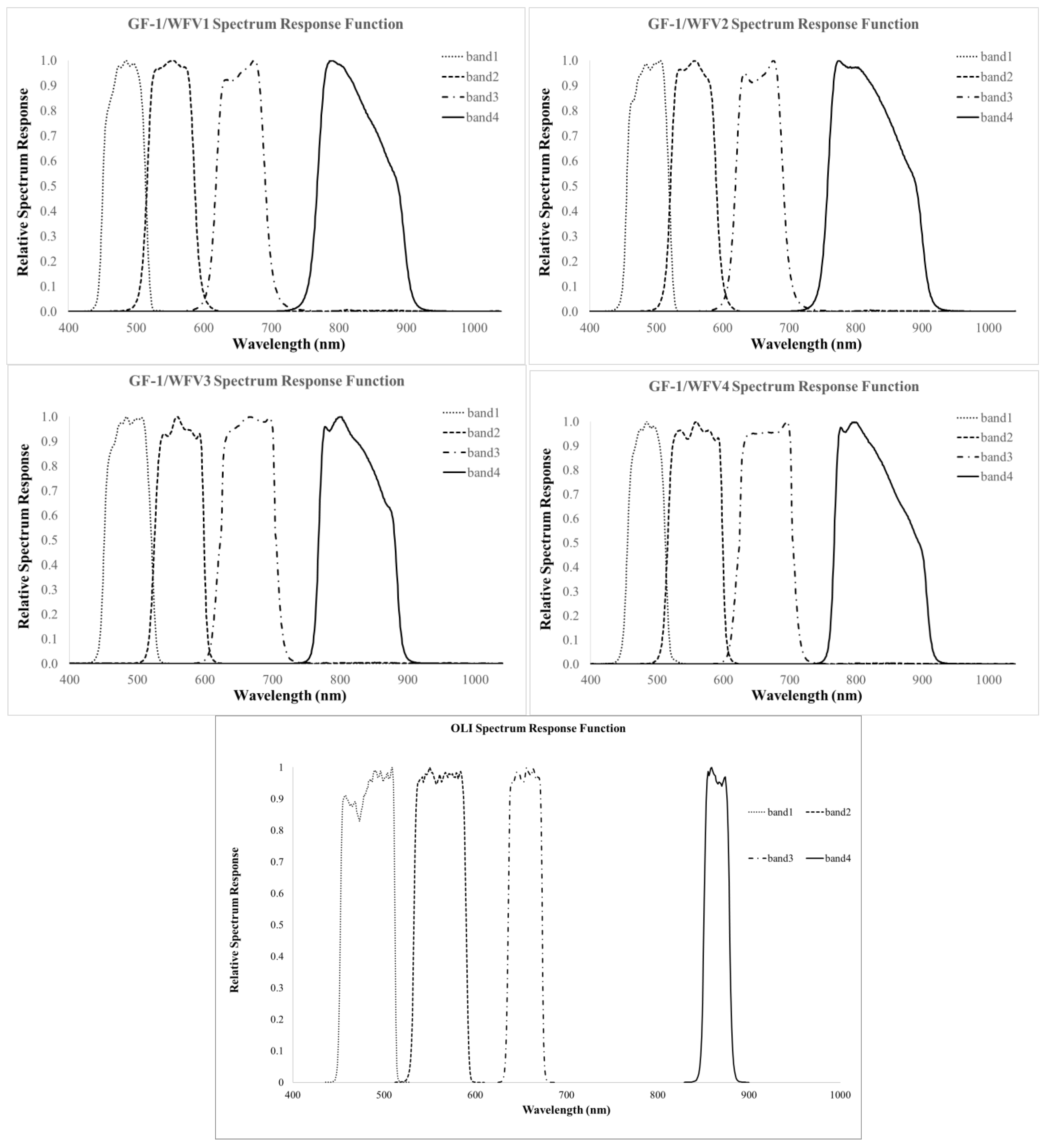
Because the spectral responses of the Landsat-8/OLI and the GF-1/WFV are different, the spectral matching between the two different sensors needs to be completed. The relative spectral response profiles of the GF-1/WFV and the Landsat-8/OLI are plotted in Figure 3. To simulate the GF-1/WFV reflectance of the calibration site, the spectral matching factors are calculated to account for the difference induced by the spectral response function between the GF-1/WFV and the Landsat-8/OLI. The spectral matching factor is defined as [1,30,31].

$$a={\displaystyle \underset{{\lambda }_1}{\overset{{\lambda }_2}{\int }}{\rho }_{\lambda }\times f_{GF}(\lambda )d\lambda }/{\displaystyle \underset{{\lambda }_3}{\overset{{\lambda }_4}{\int }}{\rho }_{\lambda }\times f_{OLI}(\lambda )d\lambda }$$

(1)

where $\text{α}$ is the spectral matching factor; $\text{λ}$ is the spectral wavelength; ${\text{ρ}}_{\text{λ}}$ is the ground-measured spectrum of the desert at the calibration site, which is plotted in Figure 4; f_GF (λ) and f_GF (λ) are the relative spectral response functions for GF-1/WFV and Landsat-8/OLI, respectively. λ₁-λ₂ is the spectral range of GF-1/WFV; λ₃-λ₄ is the spectral range of Landsat-8/OLI.

Figure 3. Relative spectral response profiles of GF-1/WFVs and Landsat-8/OLI in corresponding first to fourth wavelength regions.

Figure 3. Relative spectral response profiles of GF-1/WFVs and Landsat-8/OLI in corresponding first to fourth wavelength regions.

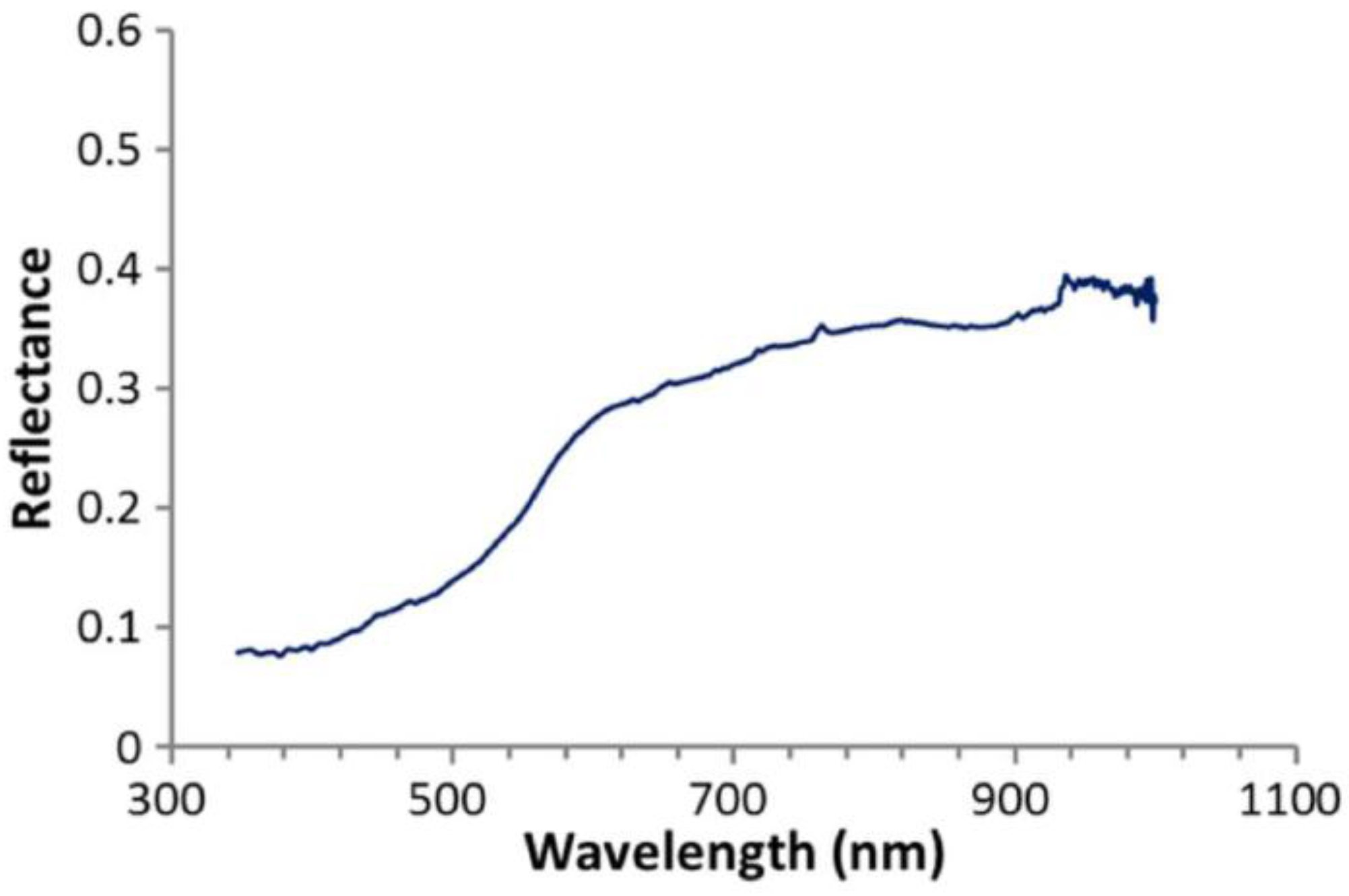
The ground-measured spectrum of the calibration site we used in this paper, which is shown in Figure 4, comes from the measurement in the Badain Jaran Desert using an SVC HR-1024 high-resolution field portable spectroradiometer on 13–14 July 2012 [1]. Based on the definition of the spectral matching factor, the spectral matching factors between the GF-1/WFV and the Landsat-8/OLI are calculated and listed in Table 4.

Figure 4. Spectra plot of the calibration site.

Figure 4. Spectra plot of the calibration site.

Table 4. Spectral matching factor between GF-1/WFV and Landsat-8/OLI.

	Sensor	Spectral Matching Factor Between GF-1/WFV and Landsat-8/OLI
Band		GF-1/WFV1	GF-1/WFV2	GF-1/WFV3	GF-1/WFV4
1		1.0012	1.0269	1.0218	1.0053
2		0.9361	0.9668	1.0068	0.9755
3		0.9990	0.9995	1.0104	1.0107
4		1.0021	1.0009	1.0019	1.0032

Table 4. Spectral matching factor between GF-1/WFV and Landsat-8/OLI.

	Sensor	Spectral Matching Factor Between GF-1/WFV and Landsat-8/OLI
Band		GF-1/WFV1	GF-1/WFV2	GF-1/WFV3	GF-1/WFV4
1		1.0012	1.0269	1.0218	1.0053
2		0.9361	0.9668	1.0068	0.9755
3		0.9990	0.9995	1.0104	1.0107
4		1.0021	1.0009	1.0019	1.0032

3.2. BRDF Fitting and Surface Reflectance of GF-1/WFV Calculation

To obtain an accurate BRDF characterization of the calibration site, the surface reflectance needs to be retrieved first. We collected 18 clean OLI images that covered the calibration site in 2013 and 2014. The selected OLI scenes and their acquisition date and solar angle are listed in Table 6. Because many clear lakes, which can be seen as dark objects, are located within the calibration site, the DO method is used to retrieve the AOD at 550 nm. The DO method is a widely used method for the atmospheric correction of remotely sensed imagery, and the advantages of the methods are its easy performance and high accuracy [32,33]. This method supposes that there is an area in the image where the reflectance is so small that it can be neglected (such as hill shading, dense vegetation, and clean water). The radiance of this area is then considered to be caused only by the atmosphere, so the AOD can be calculated through radiative transfer code, as 6S [34], and other methods, like per-pixel method [35,36]. In this study, the clear lakes in the calibration site can be considered DO to be used for atmospheric correction. The steps of AOD retrieval are as follows:

(1)

Calculate the radiance of these selected images. The radiance of the Landsat-8/OLI image can be calculated using [17]

$$L_{\lambda }=M_L{Q}_{cal}+A_L$$

(2)

where L_λ is the TOA radiance; M_λ is the band-specific multiplicative rescaling factor from the metadata (RADIANCE_MULT_BAND_X, where X is the band number); A_λ is the band-specific additive rescaling factor from the metadata (RADIANCE_ADD_BAND_X, where X is the band number); and Q_cal is the quantized and calibrated standard product pixel values (DN). The unit for L_λ is $W\cdot m^{-2}\cdot s{r}^{-1}\cdot \mu m^{-1}$.

(2)

Extract the radiance on the clear lake area for band 2. For clean water, the reflectance is low in the blue band (450–520 nm), and the radiance calculated in step (1) can be seen as atmospheric path radiance.

(3)

Set up the input parameters for the 6S model. The parameters in the 6S model include the atmospheric model, aerosol model, solar zenith and azimuth, view zenith and azimuth, wavelength, surface reflectance, and AOD. For example, the input parameters for the image on 16 April 2013 are listed in Table 5. In this table, only AOD can be changed, and every input AOD corresponds to a TOA radiance as output.

Table 5. Parameter setup for the image on 16 April 2013.

Input Parameters	Value	Notation
Atmospheric model	2	Min-latitude summer
Aerosol model	5	Shettle model for background desert aerosol
Solar zenith	144.7937	Read from header file of OLI image
Solar azimuth	55.4264	Read from header file of OLI image
View zenith	0	OLI is nadir viewing
View azimuth	0	OLI is nadir viewing
Wavelength	450–520 nm	Blue band
Surface reflectance	0	Clearwater surface is set as 0
AOD set	0.0:0.1:3.0	From 0.0 to 3.0 interval 0.1

Table 5. Parameter setup for the image on 16 April 2013.

Input Parameters	Value	Notation
Atmospheric model	2	Min-latitude summer
Aerosol model	5	Shettle model for background desert aerosol
Solar zenith	144.7937	Read from header file of OLI image
Solar azimuth	55.4264	Read from header file of OLI image
View zenith	0	OLI is nadir viewing
View azimuth	0	OLI is nadir viewing
Wavelength	450–520 nm	Blue band
Surface reflectance	0	Clearwater surface is set as 0
AOD set	0.0:0.1:3.0	From 0.0 to 3.0 interval 0.1

(4)

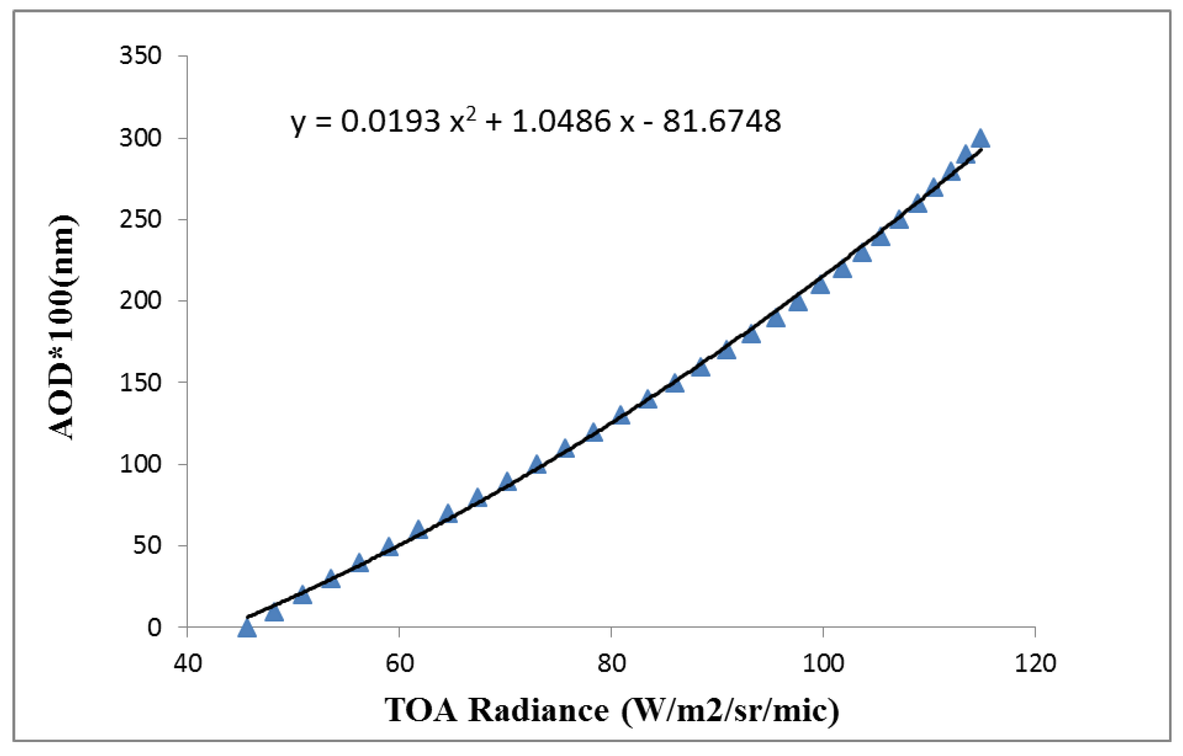
Fit the relationship between AOD and TOA radiance and interpolate the AOD with the radiance extracted in step (2). For example, for the image on 16 April 2013, the relationship between AOD and TOA radiance can be fitted as a quadratic equation, which is plotted in Figure 5. Therefore, the AOD can be interpolated using the TOA radiance retrieved from the image.

Figure 5. Example of AOD retrieval using the DO method.

Figure 5. Example of AOD retrieval using the DO method.

Finally, the AODs for all selected images can be retrieved based on the above steps and are shown in Table 6. The atmospheric effect can be corrected with the retrieved AODs for these selected images because the site is hardly influenced by human activities. After atmospheric correction, the surface reflectance of these selected images can be obtained.

Table 6. Acquisition times and retrieved AODs of the selected images.

OLI Scene	Acquisition Time (YYYY/MM/DD)	Sun Azimuth(°)	Sun Elevation(°)	Retrieved AOD at 550 nm
LC81320322013115LGN01	2013/04/25	142.9618	58.3580	0.0119
LC81320322013163LGN00	2013/06/12	130.2973	66.4286	0.2388
LC81320322013275LGN00	2013/10/02	156.5397	43.6109	0.2446
LC81320322013291LGN00	2013/10/18	160.1080	38.1122	0.0029
LC81320322013307LGN00	2013/11/03	162.2424	32.9450	0.0434
LC81320322013339LGN00	2013/12/05	162.3984	25.4647	0.0169
LC81320322013355LGN00	2013/12/21	160.8491	23.9861	0.0852
LC81330322014061LGN00	2014/03/02	150.7158	38.1367	0.1556
LC81330322014045LGN00	2014/02/14	152.8417	32.5780	0.2441
LC81330322013362LGN00	2013/12/28	159.9492	23.9154	0.0149
LC81330322013346LGN00	2013/12/12	161.8216	24.5987	0.0031
LC81330322013330LGN00	2013/11/26	162.8562	27.0349	0.0049
LC81330322013186LGN00	2013/07/05	128.8544	65.4402	0.0595
LC81330322013154LGN00	2013/06/03	132.3370	66.0213	0.3609
LC81330322013122LGN01	2013/05/02	141.3082	60.3896	0.1428
LC81330322013106LGN01	2013/04/16	144.7937	55.4264	0.3759
LC81320322014038LGN00	2014/02/07	153.8301	30.4546	0.3952
LC81320322014022LGN00	2014/01/22	156.2278	26.5810	0.0627

Table 6. Acquisition times and retrieved AODs of the selected images.

OLI Scene	Acquisition Time (YYYY/MM/DD)	Sun Azimuth(°)	Sun Elevation(°)	Retrieved AOD at 550 nm
LC81320322013115LGN01	2013/04/25	142.9618	58.3580	0.0119
LC81320322013163LGN00	2013/06/12	130.2973	66.4286	0.2388
LC81320322013275LGN00	2013/10/02	156.5397	43.6109	0.2446
LC81320322013291LGN00	2013/10/18	160.1080	38.1122	0.0029
LC81320322013307LGN00	2013/11/03	162.2424	32.9450	0.0434
LC81320322013339LGN00	2013/12/05	162.3984	25.4647	0.0169
LC81320322013355LGN00	2013/12/21	160.8491	23.9861	0.0852
LC81330322014061LGN00	2014/03/02	150.7158	38.1367	0.1556
LC81330322014045LGN00	2014/02/14	152.8417	32.5780	0.2441
LC81330322013362LGN00	2013/12/28	159.9492	23.9154	0.0149
LC81330322013346LGN00	2013/12/12	161.8216	24.5987	0.0031
LC81330322013330LGN00	2013/11/26	162.8562	27.0349	0.0049
LC81330322013186LGN00	2013/07/05	128.8544	65.4402	0.0595
LC81330322013154LGN00	2013/06/03	132.3370	66.0213	0.3609
LC81330322013122LGN01	2013/05/02	141.3082	60.3896	0.1428
LC81330322013106LGN01	2013/04/16	144.7937	55.4264	0.3759
LC81320322014038LGN00	2014/02/07	153.8301	30.4546	0.3952
LC81320322014022LGN00	2014/01/22	156.2278	26.5810	0.0627

Because the topography of the calibration site is hilly, the solar illuminations and view geometries corresponding to the slopes vary in a very large range. That is, the solar angles of the slope (the zenith and azimuth angles) and the viewing angles of the slope (the zenith and azimuth angles) are varied pixel by pixel, even though these pixels are all nadir viewed in Landsat-8/OLI imagery. For this calibration site, only if the solar illuminations and view geometries of every pixel corresponding to slopes in nadir-viewing Landsat-8/OLI imagery are known can the BRDF consequently be reconstructed. In this paper, the BRDF characterization of the calibration is reconstructed based on the BRDF fitting method developed by Zhong et al. [1]. For every pixel in remotely sensed imagery, the solar illuminations and view geometries of slopes are determined only by the slope and the aspect given the positions of the sun and the sensor. Because the slope and the aspect of the calibration site can be calculated from the DEM extracted by ZY-3/TLC, the pixel’s solar illumination and view geometries can be calculated. Notably, the slope and aspect calculated are in a local coordinate system, whereas the solar illuminations and view geometries are in the global coordinate system. Therefore, the coordinates in the global coordinate system need to be converted to those in the local coordinate system. The sun-view geometries of the local coordinate system are the real sun-view geometries of every pixel.

To keep more information, the 4-D surface (the solar zenith range of the slope, the view zenith range of the slope, the relative azimuth range of the slope, and the surface reflectance) is used to characterize the site’s BRDF instead of statistical BRDF models. In the 4-D surface, the solar zenith range of slope, the view zenith range of slope and relative azimuth range of slope are variables. Then, a lookup table (LUT) is established with the solar zenith angle of the slope, the view zenith angle of the slope and the relative azimuth angle of the slope as inputs and the surface reflectance as the output. Therefore, for any combination of the solar zenith angle of the slope, the view zenith angle of the slope and the relative azimuth angle of the slope, the corresponding surface reflectance can be obtained from the lookup table by interpolating.

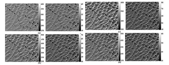
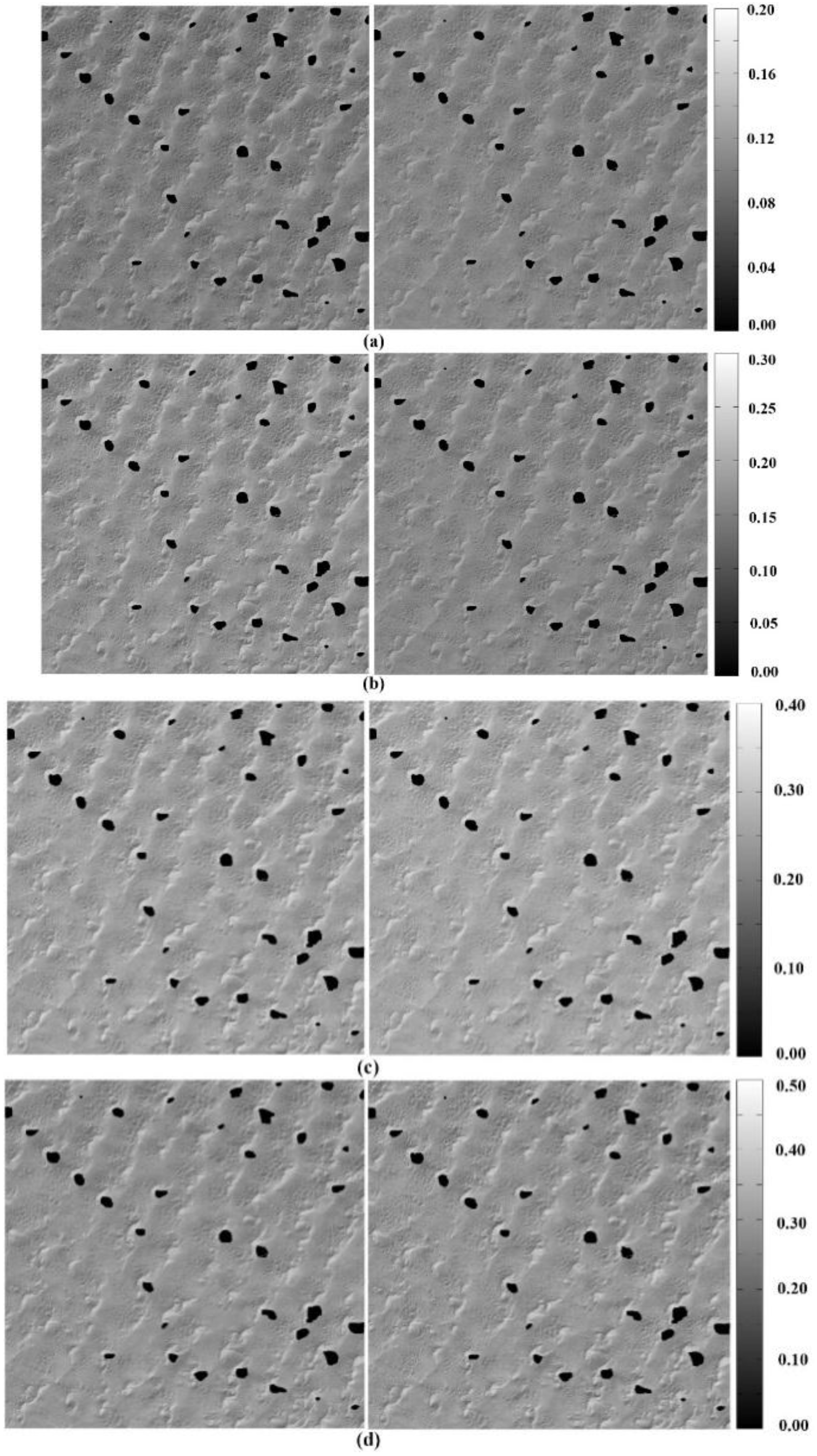
To verify the accuracy of the fitted BRDF LUT, 9 other OLI images are selected, and the surface reflectance of these chosen images is simulated using the established LUT. Figure 6 shows an example of simulation of the Landsat-8/OLI imagery on 18 March 2014. The mean surface reflectance of every image is then compared with that of the actual Landsat-8/OLI imagery (atmosphere corrected using the aforementioned DO method).

Figure 6. Example of simulated surface reflectance and its corresponding actual surface reflectance. (a) Simulated surface reflectance (left) and actual surface reflectance (right) of band 2. (b) Simulated surface reflectance (left) and actual surface reflectance (right) of band 3. (c) Simulated surface reflectance (left) and actual surface reflectance (right) of band 4. (d) Simulated surface reflectance (left) and actual surface reflectance (right) of band 5.

Figure 6. Example of simulated surface reflectance and its corresponding actual surface reflectance. (a) Simulated surface reflectance (left) and actual surface reflectance (right) of band 2. (b) Simulated surface reflectance (left) and actual surface reflectance (right) of band 3. (c) Simulated surface reflectance (left) and actual surface reflectance (right) of band 4. (d) Simulated surface reflectance (left) and actual surface reflectance (right) of band 5.

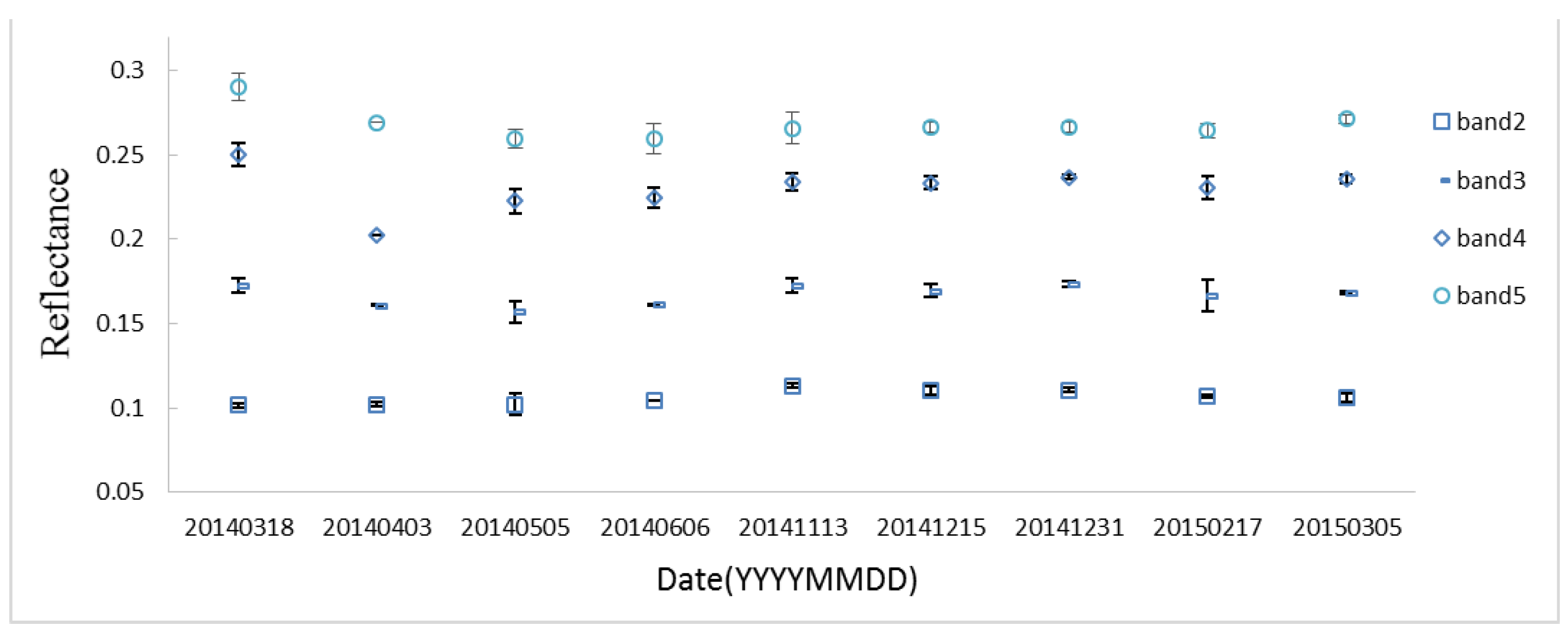
The comparison results for band 2 of all 9 OLI images between the mean simulated and actual surface reflectance are listed in Table 7, and the difference errors in percentage for bands 2–5 are plotted in Figure 7. The actual surface reflectance is from the retrieved imagery after atmospheric correction and the simulated one is simulated from the fitted BRDF characterization. The differences between the two are usually less than 5%.

Compared with the actual OLI images, the mean difference errors of the simulated images for all the 9 OLI images are 1.82% for band 2, 2.10% for band 3, 1.88% for band 4, and 1.94% for band 5. Subsequently, the derived BRDF characterization has excellent agreement with the real situation. Consequently, the BRDF characterization can be used to simulate the surface reflectance of other similar sensors, such as the GF-1/WFV, effectively.

Table 7. Comparison between actual surface reflectance and the simulated one on band 2 of OLI. Actual surface reflectance is from the retrieved imagery after atmospheric correction and the simulated one is simulated from the fitted BRDF characterization. The differences between the two are very small, so the fitted BRDF characterization can be used to simulate the surface reflectance of other similar sensors.

Acquisition Time (YYYY.MM.DD)	Actual Surface Reflectance (ρ')	Simulated Surface Reflectance (ρ')	Difference (ρ'-ρ')	Difference Error (%)
2014.03.18	0.1114	0.1128	0.0014	1.22
2014.04.03	0.1021	0.1006	−0.0015	1.49
2014.05.05	0.1021	0.1082	0.0061	5.94
2014.06.06	0.1045	0.1044	−0.0002	0.15
2014.11.13	0.1132	0.1122	−0.0010	0.86
2014.12.15	0.1105	0.1132	0.0027	2.43
2014.12.31	0.1107	0.1120	0.0013	1.19
2015.02.17	0.1167	0.1177	0.0011	0.90
2015.03.05	0.1059	0.1082	0.0023	2.20

Table 7. Comparison between actual surface reflectance and the simulated one on band 2 of OLI. Actual surface reflectance is from the retrieved imagery after atmospheric correction and the simulated one is simulated from the fitted BRDF characterization. The differences between the two are very small, so the fitted BRDF characterization can be used to simulate the surface reflectance of other similar sensors.

Acquisition Time (YYYY.MM.DD)	Actual Surface Reflectance (ρ')	Simulated Surface Reflectance (ρ')	Difference (ρ'-ρ')	Difference Error (%)
2014.03.18	0.1114	0.1128	0.0014	1.22
2014.04.03	0.1021	0.1006	−0.0015	1.49
2014.05.05	0.1021	0.1082	0.0061	5.94
2014.06.06	0.1045	0.1044	−0.0002	0.15
2014.11.13	0.1132	0.1122	−0.0010	0.86
2014.12.15	0.1105	0.1132	0.0027	2.43
2014.12.31	0.1107	0.1120	0.0013	1.19
2015.02.17	0.1167	0.1177	0.0011	0.90
2015.03.05	0.1059	0.1082	0.0023	2.20

Figure 7. Difference error between the actual and simulated surface reflectance for OLI bands 2–5 corresponding to the lines in the figure from bottom to top, respectively.

Figure 7. Difference error between the actual and simulated surface reflectance for OLI bands 2–5 corresponding to the lines in the figure from bottom to top, respectively.

In this paper, 14 scenes of GF-1/WFV (4 scenes for the GF-1/WFV1, 2 scenes for the GF-1/WFV2, 2 scenes for the GF-1/WFV3, 6 scenes for the GF-1/WFV4) that covered the calibration site are chosen. Information on these selected GF-1/WFVs images is listed in Table 8. The surface reflectance of these selected scenes is retrieved with the BRDF LUT established with the Landsat-8/OLI and DEM extracted by the ZY-3/TLC.

Table 8. Information of selected GF-1/WFVs images.

Sensor	Acquisition Time (YYYY/MM/DD)	Day of Year	Sun_Azimuth (°)	Sun_Elevation (°)
Gf-1/WFV1	2014/03/19	78	154.0470	46.6876
	2014/08/30	242	153.7930	56.8938
	2013/11/29	333	165.6380	27.5476
	2013/12/03	337	165.4560	26.8842
GF-1/WFV2	2014/09/28	271	166.1860	47.8796
	2014/01/21	22	162.2180	28.8269
GF-1/WFV3	2014/02/11	42	162.8680	33.7337
	2014/10/24	297	173.8830	37.8871
GF-1/WFV4	2014/01/18	18	167.5590	28.3773
	2014/11/13	317	177.2160	31.9344
	2013/08/09	221	152.9710	63.5083
	2013/11/18	322	173.5370	30.4243
	2014/01/26	26	166.7120	30.0972
	2013/11/26	330	173.2250	28.6828

Table 8. Information of selected GF-1/WFVs images.

Sensor	Acquisition Time (YYYY/MM/DD)	Day of Year	Sun_Azimuth (°)	Sun_Elevation (°)
Gf-1/WFV1	2014/03/19	78	154.0470	46.6876
	2014/08/30	242	153.7930	56.8938
	2013/11/29	333	165.6380	27.5476
	2013/12/03	337	165.4560	26.8842
GF-1/WFV2	2014/09/28	271	166.1860	47.8796
	2014/01/21	22	162.2180	28.8269
GF-1/WFV3	2014/02/11	42	162.8680	33.7337
	2014/10/24	297	173.8830	37.8871
GF-1/WFV4	2014/01/18	18	167.5590	28.3773
	2014/11/13	317	177.2160	31.9344
	2013/08/09	221	152.9710	63.5083
	2013/11/18	322	173.5370	30.4243
	2014/01/26	26	166.7120	30.0972
	2013/11/26	330	173.2250	28.6828

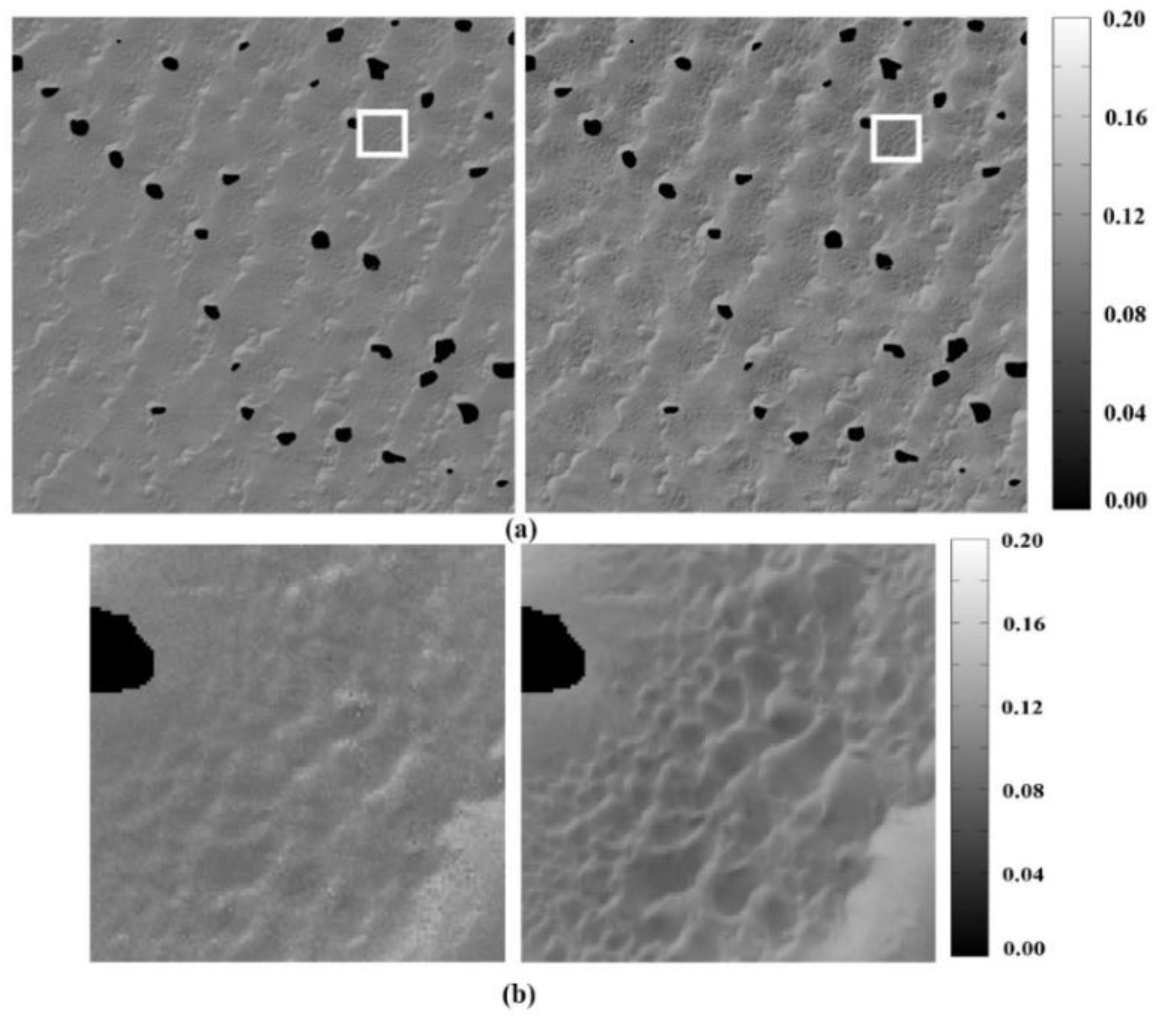
To verify the improvement of the fitted BRDF, we compare the surface reflectance simulated by the LUT established with the Landsat-8/OLI and DEM extracted by the ZY-3/TLC (new LUT) with that simulated by the LUT established with the Landsat-7/ETM+ and the ASTER GDEM (old LUT). Figure 8 shows a comparison example of the two types of surface reflectance for the GF-1/WFV1 image on 19 March 2014.

Figure 8. Comparison of the simulated surface reflectance at the blue band on 19March 2014 using the old LUT (left) and using the new LUT (right). (a) Broad view of the simulated surface reflectance and (b) close view of the highlighted area.

Figure 8. Comparison of the simulated surface reflectance at the blue band on 19March 2014 using the old LUT (left) and using the new LUT (right). (a) Broad view of the simulated surface reflectance and (b) close view of the highlighted area.

3.3. TOA Radiance Simulation and Calibration Coefficient Calculation

To simulate the TOA radiance of the GF-1/WFV images, the AOD needs to be retrieved in addition to the surface reflectance of each image. An updated retrieval algorithm by Liang et al. [37] and Zhong et al. [38] is introduced. The algorithm takes full advantage of MODIS’ multi-temporal observation capability, and its central idea is to detect the “clearest” observation during a multi-temporal window for each pixel. Therefore, only if the AODs for the “clearest” observations are known can the AODs of other “hazy” observations be interpolated from the surface reflectance of the “clearest” observations. The algorithm primarily contains the following steps:

(1)

Prepare MODIS multi-temporal images and complete the data pre-processing. The MODIS data are downloaded covering the calibration site from http://ladsweb.nascom.nasa.gov. Data pre-processing includes projection transform, subset and calibration. Then, time series MODIS TOA radiance images are prepared.

(2)

Determine the AOD for the “clearest” day. The AOD for the “clearest” day is determined through Table 3, which is calculated by the aforementioned DO method using OLI imagery.

(3)

Detect the “clearest” pixel. The long time-series images of MODIS are sorted by visual interpretation, and the “clearest” observations are selected during the temporal window for every 10° in the view zenith angles from 0° to 50° (0–10, 11–20, 21–30, 31–40 and 41–50). The images with a view zenith angle larger than 50° are not used in this study because the observation changes when the view zenith angle is larger than 50°.

(4)

Retrieve the surface reflectance of the “clearest” pixels: The surface reflectance of the “clearest” pixels can be retrieved by establishing a lookup table using the 6S model [32] because the AOD for the “clearest” pixels is known.

(5)

Fit the site’s BRDF. To better fit the BRDF characterization of the desert calibration site, the Staylor-Suttles BRDF model [39] is used, and the coefficients of the model are calculated using the calculated surface reflectance, the solar illuminations and view geometries of the “clearest” pixels. The Staylor-Suttles model is described as

$$R({\theta }_i,{\theta }_v,\varphi )=B({\mu }_v,-{\mu }_i)\frac{1+c_3{({\mu }_v{\mu }_i-\sin {\theta }_i\sin {\theta }_v\cos \varphi )}^2}{1+c_3[{({\mu }_v{\mu }_i)}^2+0.5{(\sin {\theta }_i\sin {\theta }_v)}^2]}$$

(3)

$$B({\mu }_v,-{\mu }_i)=\frac{1}{{\mu }_v{\mu }_i}[c_1+c_2{(\frac{{\mu }_v{\mu }_i}{{\mu }_v+{\mu }_i})}^N]$$

(4)

where c₁, c₂, c₃ and N are free parameters or coefficients of the model that need to be fitted, μ_i=cosθ_i, μ_v=cosθv, θ_i is the solar zenith, θv is the view zenith, and ϕ is the relative azimuth.

(6)

Retrieve the surface reflectance of all pixels. The surface reflectance of the “hazy” pixels can be calculated using the Staylor-Suttles BRDF model because the coefficients of the model are known. Then, the surface reflectance of all pixels can be retrieved.

(7)

Retrieve the AOD. The MODTRAN radiative transfer code [40] is used to retrieve the AOD of the MODIS imagery. A set of parameters needs to be set up as the MODTRAN model inputs including atmospheric model, aerosol model, surface reflectance, VIS, atmospheric water vapour content, solar zenith, view zenith, relative azimuth and TOA radiance. Every input combination corresponds to one AOD value as output.

With the above procedure, the AOD of any MODIS image can be retrieved. Because the calibration is stable, given any GF-1/WFV image, its AOD can be calculated by the corresponding MODIS image with the same transit date as the GF-1/WFV image, although the two images may have a slightly different transit time. The retrieved AODs of all selected images of the GF-1/WFV are listed in Table 9.

Table 9. Retrieved AOD for GF-1/WFV imagery.

Sensor	Acquisition Time (YYYY.MM.DD)	AOD (550 nm)
GF1/WFV1	2013.11.29	0.0574
	2013.12.03	0.1078
	2014.03.19	0.0561
	2014.08.30	0.3339
GF1/WFV2	2014.01.21	0.0558
	2014.09.28	0.0833
GF1/WFV3	2014.02.11	0.0645
	2014.10.23	0.0558
GF1/WFV4	2013.08.09	0.2251
	2013.11.18	0.0882
	2013.11.26	0.0994
	2014.01.18	0.1664
	2014.01.26	0.0883
	2014.11.13	0.0568

Table 9. Retrieved AOD for GF-1/WFV imagery.

Sensor	Acquisition Time (YYYY.MM.DD)	AOD (550 nm)
GF1/WFV1	2013.11.29	0.0574
	2013.12.03	0.1078
	2014.03.19	0.0561
	2014.08.30	0.3339
GF1/WFV2	2014.01.21	0.0558
	2014.09.28	0.0833
GF1/WFV3	2014.02.11	0.0645
	2014.10.23	0.0558
GF1/WFV4	2013.08.09	0.2251
	2013.11.18	0.0882
	2013.11.26	0.0994
	2014.01.18	0.1664
	2014.01.26	0.0883
	2014.11.13	0.0568

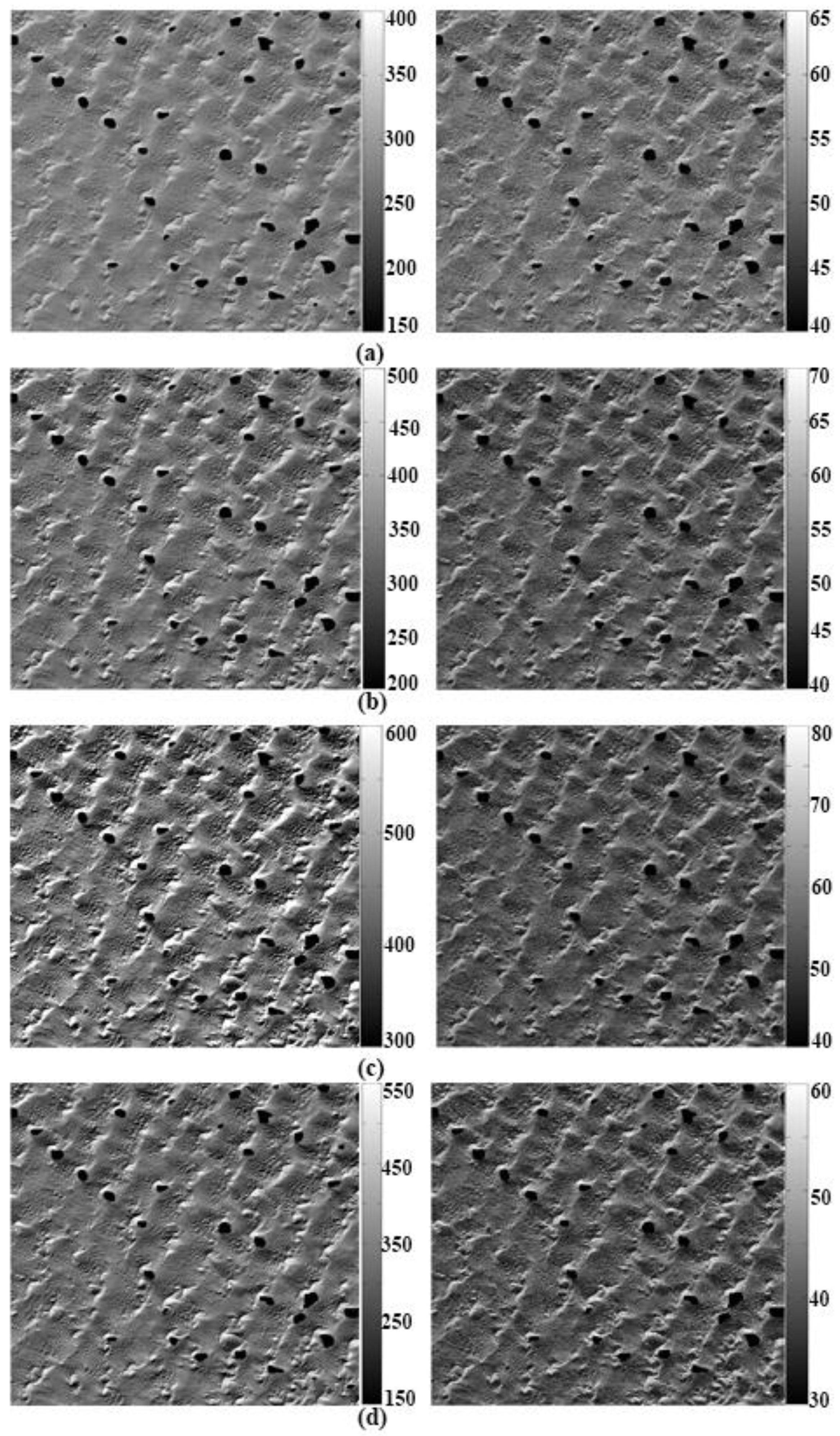
With the derived GF-1/WFV surface reflectance and the AOD retrieved by MODIS imagery, the TOA radiance of the GF-1/WFV can be calculated using the 6S model. The mean TOA radiance and DN for every GF-1/WFV image are listed in Table 10. An example of the simulated TOA radiance and its corresponding $DN$ for the GF-1/WFV image on 25 April 2013 is shown in Figure 9.

Table 10. Mean TOA radiance and DN for every GF-1/WFV image.

Sensor	Date (YYYY.MM.DD)	Band 1		Band 2		Band 3		Band 4
		DN	TOA	DN	TOA	DN	TOA	DN	TOA
GF1/WFV1	2013.11.29	286.37	52.84	338.09	50.76	426.49	54.05	309.02	41.86
	2013.12.03	276.98	53.09	328.47	50.35	418.38	52.71	306.75	40.54
	2014.03.19	416.55	74.00	513.40	75.07	662.84	89.98	476.86	65.25
	2014.08.30	438.81	87.02	548.11	88.48	714.68	95.42	498.47	74.05
GF1/WFV2	2014.01.21	275.05	51.24	335.62	50.87	437.26	53.53	321.29	40.43
	2014.09.28	393.90	66.80	504.41	71.86	652.25	81.79	456.83	63.83
GF1/WFV3	2014.02.11	323.60	57.75	367.65	63.85	460.96	70.20	354.98	56.16
	2014.10.23	331.13	63.06	385.90	68.16	491.87	72.75	372.63	57.42
GF1/WFV4	2013.08.09	439.24	89.20	522.10	99.83	647.38	117.70	494.37	89.93
	2013.11.18	312.47	59.26	346.12	64.86	415.75	72.39	327.41	57.74
	2013.11.26	283.80	50.05	313.88	61.69	383.11	68.57	301.64	54.62
	2014.01.18	312.47	58.41	346.12	62.77	415.75	69.02	327.41	54.98
	2014.01.26	296.12	59.69	327.65	65.64	399.93	73.73	321.66	58.96
	2014.11.13	321.17	60.55	360.54	66.78	433.87	74.95	347.77	59.79

Table 10. Mean TOA radiance and DN for every GF-1/WFV image.

Sensor	Date (YYYY.MM.DD)	Band 1		Band 2		Band 3		Band 4
		DN	TOA	DN	TOA	DN	TOA	DN	TOA
GF1/WFV1	2013.11.29	286.37	52.84	338.09	50.76	426.49	54.05	309.02	41.86
	2013.12.03	276.98	53.09	328.47	50.35	418.38	52.71	306.75	40.54
	2014.03.19	416.55	74.00	513.40	75.07	662.84	89.98	476.86	65.25
	2014.08.30	438.81	87.02	548.11	88.48	714.68	95.42	498.47	74.05
GF1/WFV2	2014.01.21	275.05	51.24	335.62	50.87	437.26	53.53	321.29	40.43
	2014.09.28	393.90	66.80	504.41	71.86	652.25	81.79	456.83	63.83
GF1/WFV3	2014.02.11	323.60	57.75	367.65	63.85	460.96	70.20	354.98	56.16
	2014.10.23	331.13	63.06	385.90	68.16	491.87	72.75	372.63	57.42
GF1/WFV4	2013.08.09	439.24	89.20	522.10	99.83	647.38	117.70	494.37	89.93
	2013.11.18	312.47	59.26	346.12	64.86	415.75	72.39	327.41	57.74
	2013.11.26	283.80	50.05	313.88	61.69	383.11	68.57	301.64	54.62
	2014.01.18	312.47	58.41	346.12	62.77	415.75	69.02	327.41	54.98
	2014.01.26	296.12	59.69	327.65	65.64	399.93	73.73	321.66	58.96
	2014.11.13	321.17	60.55	360.54	66.78	433.87	74.95	347.77	59.79

The calibration coefficients for the GF-1/WFV can be calculated using

$$L=DN\cdot g+b$$

(5)

where L is the TOA radiance, g is the gain, b is the offset, DN is the digital reading of the imagery. The unit for L and b is $W\cdot m^{-2}\cdot s{r}^{-1}\cdot \mu m^{-1}$.

In this paper, parameter L is simulated, parameter b can be used prelaunch to offset (0 for each band), and the parameter DN can be read from the GF-1/WFV image. Then, the parameters of every scene are calculated. The results are shown in Table 11.

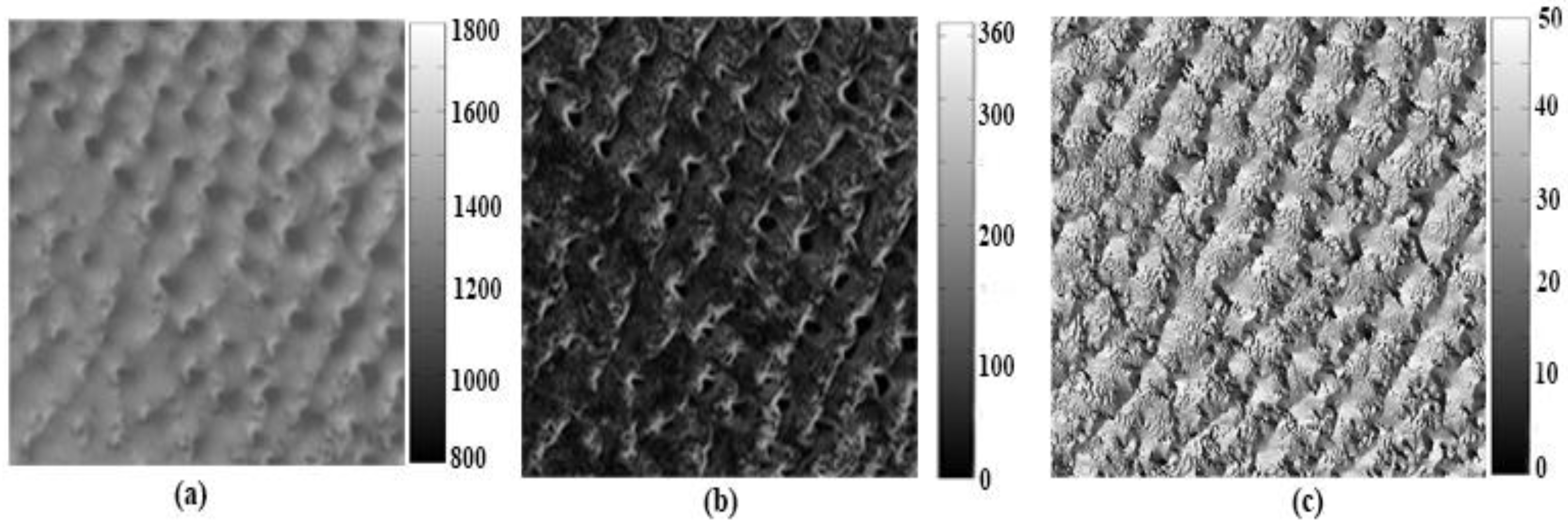
Figure 9. Example of the simulated TOA radiance and its corresponding DN of GF-1/WFV image on 11 February 2014. (a) Simulated TOA (right) and DN (left) of band 1. (b) Simulated TOA (right) and DN (left) of band 2. (c) Simulated TOA (right) and DN (left) of band 3. (d) Simulated TOA (right) and DN (left) of band 4.

Figure 9. Example of the simulated TOA radiance and its corresponding DN of GF-1/WFV image on 11 February 2014. (a) Simulated TOA (right) and DN (left) of band 1. (b) Simulated TOA (right) and DN (left) of band 2. (c) Simulated TOA (right) and DN (left) of band 3. (d) Simulated TOA (right) and DN (left) of band 4.

Table 11. Calibration coefficients for GF-1/WFV.

Sensor	Band 1		Band 2		Band 3		Band 4
GF1/WFV1	Gain	Bias	Gain	Bias	Gain	Bias	Gain	Bias
20131129	0.1765	0.000	0.1465	0.000	0.1234	0.000	0.1320	0.000
20131203	0.1829	0.000	0.1491	0.000	0.1224	0.000	0.1289	0.000
20140319	0.1693	0.000	0.1432	0.000	0.1233	0.000	0.1347	0.000
20140830	0.1901	0.000	0.1571	0.000	0.1314	0.000	0.1474	0.000
Mean	0.1797	0.000	0.1490	0.000	0.1251	0.000	0.1358	0.000
Sensor	Band 1		Band 2		Band 3		Band 4
GF1/WFV2	Gain	Bias	Gain	Bias	Gain	Bias	Gain	Bias
20140121	0.1734	0.000	0.1463	0.000	0.1197	0.000	0.1257	0.000
20140928	0.1679	0.000	0.1424	0.000	0.1213	0.000	0.1352	0.000
Mean	0.1707	0.000	0.1444	0.000	0.1205	0.000	0.1304	0.000
Sensor	Band 1		Band 2		Band 3		Band 4
GF1/WFV3	Gain	Bias	Gain	Bias	Gain	Bias	Gain	Bias
20140211	0.1675	0.000	0.1631	0.000	0.1400	0.000	0.1464	0.000
20141023	0.1739	0.000	0.1668	0.000	0.1415	0.000	0.1500	0.000
Mean	0.1707	0.000	0.1649	0.000	0.1407	0.000	0.1482	0.000
Sensor	Band 1		Band 2		Band 3		Band 4
GF1/WFV4	Gain	Bias	Gain	Bias	Gain	Bias	Gain	Bias
20130809	0.1965	0.000	0.1928	0.000	0.1746	0.000	0.1828	0.000
20131118	0.1740	0.000	0.1708	0.000	0.1555	0.000	0.1568	0.000
20131126	0.1850	0.000	0.1795	0.000	0.1600	0.000	0.1611	0.000
20140118	0.1728	0.000	0.1661	0.000	0.1486	0.000	0.1494	0.000
20140126	0.1847	0.000	0.1822	0.000	0.1642	0.000	0.1624	0.000
20141113	0.1724	0.000	0.1687	0.000	0.1545	0.000	0.1533	0.000
Mean	0.1809	0.000	0.1767	0.000	0.1596	0.000	0.1610	0.000

Table 11. Calibration coefficients for GF-1/WFV.

Sensor	Band 1		Band 2		Band 3		Band 4
GF1/WFV1	Gain	Bias	Gain	Bias	Gain	Bias	Gain	Bias
20131129	0.1765	0.000	0.1465	0.000	0.1234	0.000	0.1320	0.000
20131203	0.1829	0.000	0.1491	0.000	0.1224	0.000	0.1289	0.000
20140319	0.1693	0.000	0.1432	0.000	0.1233	0.000	0.1347	0.000
20140830	0.1901	0.000	0.1571	0.000	0.1314	0.000	0.1474	0.000
Mean	0.1797	0.000	0.1490	0.000	0.1251	0.000	0.1358	0.000
Sensor	Band 1		Band 2		Band 3		Band 4
GF1/WFV2	Gain	Bias	Gain	Bias	Gain	Bias	Gain	Bias
20140121	0.1734	0.000	0.1463	0.000	0.1197	0.000	0.1257	0.000
20140928	0.1679	0.000	0.1424	0.000	0.1213	0.000	0.1352	0.000
Mean	0.1707	0.000	0.1444	0.000	0.1205	0.000	0.1304	0.000
Sensor	Band 1		Band 2		Band 3		Band 4
GF1/WFV3	Gain	Bias	Gain	Bias	Gain	Bias	Gain	Bias
20140211	0.1675	0.000	0.1631	0.000	0.1400	0.000	0.1464	0.000
20141023	0.1739	0.000	0.1668	0.000	0.1415	0.000	0.1500	0.000
Mean	0.1707	0.000	0.1649	0.000	0.1407	0.000	0.1482	0.000
Sensor	Band 1		Band 2		Band 3		Band 4
GF1/WFV4	Gain	Bias	Gain	Bias	Gain	Bias	Gain	Bias
20130809	0.1965	0.000	0.1928	0.000	0.1746	0.000	0.1828	0.000
20131118	0.1740	0.000	0.1708	0.000	0.1555	0.000	0.1568	0.000
20131126	0.1850	0.000	0.1795	0.000	0.1600	0.000	0.1611	0.000
20140118	0.1728	0.000	0.1661	0.000	0.1486	0.000	0.1494	0.000
20140126	0.1847	0.000	0.1822	0.000	0.1642	0.000	0.1624	0.000
20141113	0.1724	0.000	0.1687	0.000	0.1545	0.000	0.1533	0.000
Mean	0.1809	0.000	0.1767	0.000	0.1596	0.000	0.1610	0.000

3.4. Verification of the Updated Calibration Method Using the GF-1/WFV Data

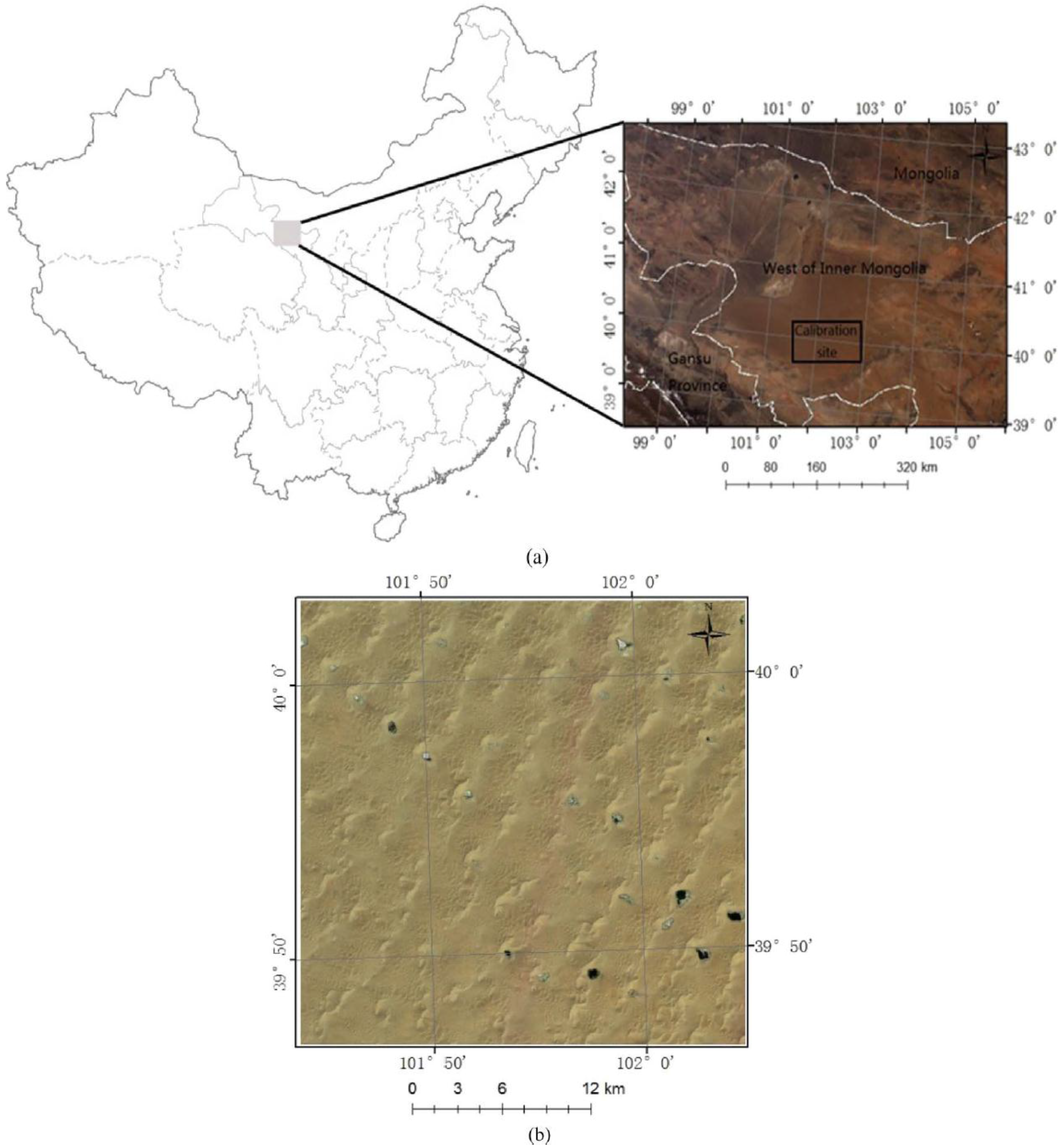
The calibration coefficients in this paper are slightly different from those published by CRESDA, so further verification is needed. Generally speaking, the Working Group on Calibration and Validation of the Committee on Earth Observation Satellites always take ground measurements of land-surface spectra and atmospheric parameters at the Dunhuang test site, which can be used to verify cross-calibrated results as actual data. The Dunhuang test site, located in Gansu Province, China, is one of the China Radiometric Calibration Sites for the vicarious calibration of Chinese space-borne sensors. The site is spatially uniform, with a coefficient of variation less than 2% of the spectral reflectance over the 10 km-by-10 km central region [8]. Unfortunately, synchronized ground-measurement data are not retrieved, so the OLI images covering the Dunhuang test site are used as reference data for validation. The procedure is carried out as follows:

(1)

Choose image pairs of the GF-1/WFVs and the Landsat-8/OLI with a similar transit time at the Dunhuang test site. Information on the chosen image pairs is listed in Table 12.

(2)

Calculate the TOA reflectance of these GF-1/WFVs images using the calibration coefficients given by CRESDA. The TOA radiance of the GF-1/WFV can be calculated using Equation (5), and the TOA reflectance of the GF-1/WFV can be calculated using Equation (6).

$${\rho }_{\lambda }=\frac{\pi L_{\lambda }{d}^2}{ESU{N}_{\lambda }\cdot \sin ({\theta }_{SE})}$$

(6)

where ${\text{ρ}}_{\text{λ}}$ is the TOA reflectance; $L_{\text{λ}}$ is the TOA radiance; d is the distance of the earth; θ_SE is the solar elevation; and ESUN_λ is the solar irradiance at the top of atmosphere, listed in Table 13.

Table 12. Information of the chosen image pairs of GF-1/WFVs and Landsat-8/OLI.

Sensor	Acquiring Date of GF-1/WFVs (YYYYMMDD)	Acquiring Date of OLI (YYYYMMDD)	Solar Zenith of GF-1/WFVs (°)	Solar Zenith of OLI (°)	View Zenith of GF-1/WFVs (°)	View Zenith of OLI (°)	Relative Azimuth of GF-1/WFVs (°)	Relative Azimuth of OLI (°)
WFV1	20140312	20140314	46.0999	47.2203	26.6714	0.0000	53.1060	149.3809
WFV2	20140815	20140812	27.6772	31.1131	8.8375	0.0000	48.3420	137.9205
WFV3	20140212	20140217	55.9372	56.3834	8.7908	0.0000	120.5010	152.6038
WFV4	20140111	20140116	65.5926	64.4100	32.8268	0.0000	116.1370	157.3043

Table 12. Information of the chosen image pairs of GF-1/WFVs and Landsat-8/OLI.

Sensor	Acquiring Date of GF-1/WFVs (YYYYMMDD)	Acquiring Date of OLI (YYYYMMDD)	Solar Zenith of GF-1/WFVs (°)	Solar Zenith of OLI (°)	View Zenith of GF-1/WFVs (°)	View Zenith of OLI (°)	Relative Azimuth of GF-1/WFVs (°)	Relative Azimuth of OLI (°)
WFV1	20140312	20140314	46.0999	47.2203	26.6714	0.0000	53.1060	149.3809
WFV2	20140815	20140812	27.6772	31.1131	8.8375	0.0000	48.3420	137.9205
WFV3	20140212	20140217	55.9372	56.3834	8.7908	0.0000	120.5010	152.6038
WFV4	20140111	20140116	65.5926	64.4100	32.8268	0.0000	116.1370	157.3043

Table 13. Solar irradiance at the top of atmosphere of GF-1/WFVs.

Sensor	Band	ESUNλ
WFV1	1	1969.7
	2	1859.7
	3	1560.1
	4	1078.1
WFV2	1	1957.3
	2	1857.6
	3	1560.1
	4	1079.3
WFV3	1	1960.1
	2	1854.2
	3	1557.1
	4	1080.7
WFV4	1	1969.2
	2	1855.7
	3	1557.7
	4	1078.0

Table 13. Solar irradiance at the top of atmosphere of GF-1/WFVs.

Sensor	Band	ESUNλ
WFV1	1	1969.7
	2	1859.7
	3	1560.1
	4	1078.1
WFV2	1	1957.3
	2	1857.6
	3	1560.1
	4	1079.3
WFV3	1	1960.1
	2	1854.2
	3	1557.1
	4	1080.7
WFV4	1	1969.2
	2	1855.7
	3	1557.7
	4	1078.0

(3)

Calculate the TOA reflectance of the GF-1/WFVs images using the calibration coefficients retrieved in this paper. The TOA reflectance of the GF-1/WFV can be calculated using Equations (5) and (6).

(4)

Calculate the TOA reflectance of these OLI images using the given calibration coefficients. The TOA reflectance of OLI can be calculated using [17]

$${\rho }_{\lambda }=(M_{\text{ρ}}{Q}_{cal}+A_{\text{ρ}})/\text{sin}\left({\theta }_{SE}\right)$$

(7)

where ρ_λ is the TOA reflectance; M_ρ is the band-specific multiplicative rescaling factor from the metadata (REFLECTANCE_MULT_BAND_X, where X is the band number); A_ρ is the band-specific additive rescaling factor from the metadata (REFLECTANCE_ADD_BAND_X, where X is the band number); Q_cal is the quantized and calibrated standard product pixel values (DN); and θ_SE is solar elevation.

(5)

Compare the three sets of TOA reflectance. The comparison results are listed in Table 14.

Compared with the TOA reflectance from synchronized OLI images, all errors of the TOA reflectance calculated using the calibration coefficients in this paper are less than 5%, and more than half of those are less than 3%, much less than that calculated with the calibration coefficients given by CRESDA, whose error could reach 20%. Consequently, the calibration coefficients retrieved in this paper have high accuracy, and the cross-calibration method performs excellently for the GF-1/WFVs. Therefore, the updated cross-calibration method performs very well for different GF-1/WFV cameras. Compared with the given calibration coefficients provided once every year, the updated cross-calibration method can provide as many calibration coefficients as possible only if there is GF-1/WFV imagery at the Badan Jaran Desert calibration site without cloud contamination. The updated cross-calibration method can be made a routine procedure for cross-calibrating GF-1/WFVs.

Table 14. GF-1/WFV cross-calibration validation results.

Sensor	Date (YYYYMMDD)	Band	DN	GCC *	CCC $	TOA reflectance by GCC	TOA reflectance by CCC	TOA reflectance by OLI	Error by GCC (%)	Error by CCC (%)
WFV1	20140312	1	573.9939	0.2004	0.1693	0.2646	0.2370	0.2295	20.52	3.26
		2	657.9767	0.1648	0.1432	0.2642	0.2295	0.2279	15.94	0.74
		3	718.4975	0.1243	0.1233	0.2594	0.2573	0.2556	1.47	0.66
		4	475.5688	0.1563	0.1347	0.3124	0.2692	0.2773	12.67	2.90
WFV2	20140815	1	629.9536	0.1733	0.1679	0.1939	0.1878	0.1944	0.29	3.40
		2	739.1819	0.1383	0.1424	0.1967	0.2025	0.2050	4.06	1.21
		3	798.6314	0.1122	0.1213	0.2122	0.2294	0.2283	7.07	0.47
		4	494.6433	0.1391	0.1352	0.2396	0.2329	0.2434	1.53	4.30
WFV3	20140212	1	442.7085	0.1745	0.1675	0.2337	0.2122	0.2173	7.54	2.35
		2	458.7962	0.1514	0.1631	0.1988	0.2264	0.2196	9.48	3.09
		3	498.3198	0.1257	0.1400	0.2256	0.2513	0.2467	8.53	1.87
		4	352.0519	0.1462	0.1464	0.2671	0.2675	0.2702	1.12	0.99
WFV4	20140111	1	417.5617	0.1713	0.1724	0.2048	0.2066	0.1983	3.29	4.20
		2	430.0000	0.1600	0.1687	0.2008	0.2084	0.1995	3.22	4.47
		3	436.7456	0.1497	0.1545	0.2255	0.2239	0.2148	4.98	4.20
		4	311.8841	0.1435	0.1533	0.2269	0.2362	0.2325	2.41	1.60

* GCC is the abbreviation of given calibration coefficients; ^$ CCC is the abbreviation of cross-calibration coefficients.

Table 14. GF-1/WFV cross-calibration validation results.

Sensor	Date (YYYYMMDD)	Band	DN	GCC *	CCC $	TOA reflectance by GCC	TOA reflectance by CCC	TOA reflectance by OLI	Error by GCC (%)	Error by CCC (%)
WFV1	20140312	1	573.9939	0.2004	0.1693	0.2646	0.2370	0.2295	20.52	3.26
		2	657.9767	0.1648	0.1432	0.2642	0.2295	0.2279	15.94	0.74
		3	718.4975	0.1243	0.1233	0.2594	0.2573	0.2556	1.47	0.66
		4	475.5688	0.1563	0.1347	0.3124	0.2692	0.2773	12.67	2.90
WFV2	20140815	1	629.9536	0.1733	0.1679	0.1939	0.1878	0.1944	0.29	3.40
		2	739.1819	0.1383	0.1424	0.1967	0.2025	0.2050	4.06	1.21
		3	798.6314	0.1122	0.1213	0.2122	0.2294	0.2283	7.07	0.47
		4	494.6433	0.1391	0.1352	0.2396	0.2329	0.2434	1.53	4.30
WFV3	20140212	1	442.7085	0.1745	0.1675	0.2337	0.2122	0.2173	7.54	2.35
		2	458.7962	0.1514	0.1631	0.1988	0.2264	0.2196	9.48	3.09
		3	498.3198	0.1257	0.1400	0.2256	0.2513	0.2467	8.53	1.87
		4	352.0519	0.1462	0.1464	0.2671	0.2675	0.2702	1.12	0.99
WFV4	20140111	1	417.5617	0.1713	0.1724	0.2048	0.2066	0.1983	3.29	4.20
		2	430.0000	0.1600	0.1687	0.2008	0.2084	0.1995	3.22	4.47
		3	436.7456	0.1497	0.1545	0.2255	0.2239	0.2148	4.98	4.20
		4	311.8841	0.1435	0.1533	0.2269	0.2362	0.2325	2.41	1.60

* GCC is the abbreviation of given calibration coefficients; ^$ CCC is the abbreviation of cross-calibration coefficients.

4. Discussion

Overall, the updated cross-calibration method is useful for GF-1/WFV, although the wide swath coverage and much larger view angles of GF-1/WFVs made them difficult to be cross-calibrated using similar sensors like Landsat series, which are mostly observing the earth nadir. The Badain Jaran Desert is selected as the calibration site for it has a homogeneous surface material, which is sand, but the topography is hilly. This affords a wide range of local slopes and aspects of the same basic material, a natural data set for characterizing the material BRDF. The well-calibrated Landsat-8/OLI and DEM data extracted by the ZY-3/TLC are used together to retrieve the BRDF characterizing of the calibration site and cross-calibrate GF-1/WFVs. The updated cross-calibration method primarily aims at 10-bit remote sensing data, compared with the cross-calibration method proposed by Zhong et al. [1], which is primarily aimed at 8-bit data. With the development of remote sensing technology and the increase in remote sensing application requirements, higher radiometric quantization data may be used more widely because it can convey more details of the surface. Therefore, the updated method has greater application potential. The updated cross-calibration method uses DEM data extracted by the ZY-3/TLC, which has a higher spatial resolution than the ASTER GDEM product, so more accurate cross-calibration results can be obtained with the updated method. The method takes advantage of a site with uniform surface material and a natural topographic variation. Sensors with a wide field of view provide challenges for cross-calibration with a narrow field of view sensors. Due to the topography, the near-nadir Landsat-8/OLI observations actually show the material at a wide range of illumination and view angles. These observations and DEM data can be used to develop a model of the calibration site’s BRDF that covers most of the illumination and view-angle range of the sensor data with wide field of view, as the GF-1/WFV. Therefore, the updated cross-calibration is innovative. Compared to the given calibration coefficients provided once every year, the cross-calibration method can provide only if there is GF-1/WFV imagery at Badain Jaran Desert calibration site without cloud and haze contamination, so the updated cross-calibration method can be proposed as a routine procedure for cross-calibrating GF_1/WFVs. Additionally, the method has broad application prospects; it can be used for other Chinese sensors with medium or high spatial resolutions.

In this study, only 8 GF-1/WFVs images are selected (Table 8) and used to be cross-calibrated because the GF-1/WFVs data is limited at Badain Jaran Desert calibration site, so not enough calibration coefficients are obtained. Thus, the accuracy of the calibration result may be affected because the mean calibration coefficients are used in validation. Furthermore, not many synchronized Landsat-8/OLI and GF-1/WFV images have been accumulated over the past two years, so only limited cross-calibration coefficients were calculated. In addition, the validation of the updated method is limited by insufficient synchronized ground measurements, and further validation is required in the near future.

5. Conclusions

In this paper, an updated version of the cross-calibration method proposed by Zhong et al .[1] is developed for better cross-calibrating GF-1/WFV. Two improvements in the updated method were made specifically for the new characteristics of the GF-1/WFV. On one hand, the GF-1/WFV has a wide swath coverage and a band setting similar to that of the HJ-1/CCD, so the cross-calibration method for the data with wide swath and large viewing angles, such as the HJ-1/CCD, proposed by Zhong et al. [1] can be applied to the GF-1/WFV. However, the GF-1/WFV has a radiometric quantization of 10 bit, so the former, using Landsat-7/ETM+ with only 8 bit radiometric quantization, is not good enough for GF-1/WFV cross-calibration. On the other hand, the spatial resolution of the GF-1/WFV is 16 m, which is much higher than that of the ASTER GDEM product (~ 120 m), so the DEM with 16 m resolution extracted from the ZY-3/TLC is used to update the method. With the two improvements, the newly built LUT can better simulate the BRDF characterization of the calibration site. Compared with the surface reflectance of selected OLI images after atmospheric correction (actual surface reflectance), the absolute values of the difference in the simulated images are 1.82% for band 2, 2.10% for band 3, 1.88% for band 4, and 1.94% for band 5. Compared with the surface reflectance retrieved by the old BRDF LUT, the result retrieved by the new one has a similar texture and more details. Compared with the TOA reflectance from synchronized OLI images, all errors of the TOA reflectance calculated with the calibration coefficients retrieved in this paper are less than 5%, much less than those calculated with the calibration coefficients given by CRESDA.