Article

Rice Fields Mapping in Fragmented Area Using Multi-Temporal HJ-1A/B CCD Images

1
Institute of Remote Sensing and Information Application, Zhejiang University, Hangzhou 310058, China
2
Institute of Remote Sensing and Earth Sciences, Hangzhou Normal University, Hangzhou 311121, China
*
Author to whom correspondence should be addressed.
Remote Sens. 2015, 7(4), 3467-3488; https://doi.org/10.3390/rs70403467
Submission received: 30 December 2014 / Accepted: 17 March 2015 / Published: 24 March 2015
(This article belongs to the Special Issue Recent Advances in Remote Sensing for Crop Growth Monitoring)

Abstract

:
Rice is one of the most important crops in the world; meanwhile, the rice field is also an important contributor to greenhouse gas methane emission. Therefore, it is important to get an accurate estimation of rice acreage for both food production and climate change related studies. The eastern plain region is one of the major single-cropped rice (SCR) growing areas in China. Subjected to the topography and intensified human activities, the rice fields are generally fragmented and irregular. How remote sensing can meet this challenge to accurately estimate the acreage of the rice in this region using medium-resolution imagery is the topic of this study. In this study, the applicability of the Chinese HJ-1A/B satellites and a two-band enhanced vegetation index (EVI2) was investigated. Field campaigns were carried out during the rice growing season and ground-truth data were collected for classification accuracy assessments in 2012. A stepwise classification strategy utilizing the EVI2 signatures during key phenology stages, i.e., the transplanting and the vegetative to reproductive transition phases, of the SCR was proposed, and the overall classification accuracy was 91.7%. The influence of the mixed pixel and boundary effects to classification accuracy was also investigated. This work demonstrates that the Chinese HJ-1A/B data are suitable data source to estimating SCR cropping area under complex land cover composition.

Graphical Abstract

1. Introduction

Rice is one of the most important crops in the world and provides the main source of energy for more than half of the world population [1]. Additionally, the seasonally flooded rice fields contribute about 5%–19% of total global methane emission, an important greenhouse gas source, to the atmosphere [2,3]. China produced about one third of the world’s rice on about one fifth of the world’s paddy rice land [4]. During the past two decades, the arable land in China declined at a speed of 0.25 million hectares per year [5]. The trend was more obvious in the eastern plain region of China, where intensified human activities have changed the land use and land cover (LULC) patterns dramatically in the last decades. This region has long been one of the major rice growing areas in China, and the cultivar is dominated by the single-cropped rice (SCR). From the food safety, ecological and policy making points of view, a timely and efficient monitoring and mapping of rice cropping area is critical [6,7]. Conventionally, the local government usually estimates the cropping area of rice by field survey; however, it is time-consuming and costly. As a powerful alternative, remote sensing has proved its effectiveness in estimating rice cropping areas from regional to global scales [8,9,10].
In the literature, many different kinds of optical remote sensing data, e.g., the Advanced Very High Resolution Radiometer (AVHRR), Moderate Resolution Imaging Spectroradiometer (MODIS), SPOT VEGETATION and Landsat-MSS, and techniques have been applied in rice cropping area estimating practices [7,8,11,12,13]. The data mentioned above have demonstrated advantages in rice monitoring at regional to global scales due to wide range of coverage and relative long data archiving. However, coarse resolution satellite data is not suitable for precise rice crop mapping in the eastern plain region of China because the rice fields in this region are relatively small, irregular, and fragmented by well-developed roads and dense water networks, and generally mixed with other land cover types. As a consequence, the mixed-pixel problem is prominent and induces temporal uncertainty in discriminating the spectral signatures of rice and the other land cover types [6].
Middle to high spatial resolution satellite data, e.g., Landsat TM/ETM+/OLI, SPOT and China Brazil Earth Resources Satellite (CBERS), are promising in capturing small patches of crop fields [14,15]. However, the cost and relatively long revisit cycles partially offset their advantages in spatial resolution. Specifically, the cloud cover during monsoon season, which is partially overlapped with the major growing season of the SCR, makes it more difficult to obtain qualified remote sensing imageries [16,17]. For applications where the rice phenology information is critically needed, the satellite data with acceptable spatial resolution and more frequent revisit cycle should be more desirable.
The small sun-synchronous satellites for environment and disaster monitoring and forecasting (HJ-1A/B) of China were launched in 2008. HJ-1A/B satellites have a spatial resolution of 30 m and a revisit cycle of four days (the revisit cycle of the constellation is 2 days), with imaging swath of 700 km. The CCD camera onboard HJ-1A/B includes four bands, i.e., blue, green, red and near-infrared, and the spectral range is 0.43–0.90 μm. HJ-1A/B CCD data have been applied in rice area estimation [18,19] and yield prediction [20]. In this study, however, it is our interest to explore the potential of using HJ-1A/B data to extract small, irregular SCR growing area in the eastern plain region of China, where the mixed-pixel problem is serious as mentioned above. Specifically, it is our interest to take advantage of its high revisit feature of the HJ-1A/B data to capture the key phenology spectral signatures of the SCR to facilitate the classification.
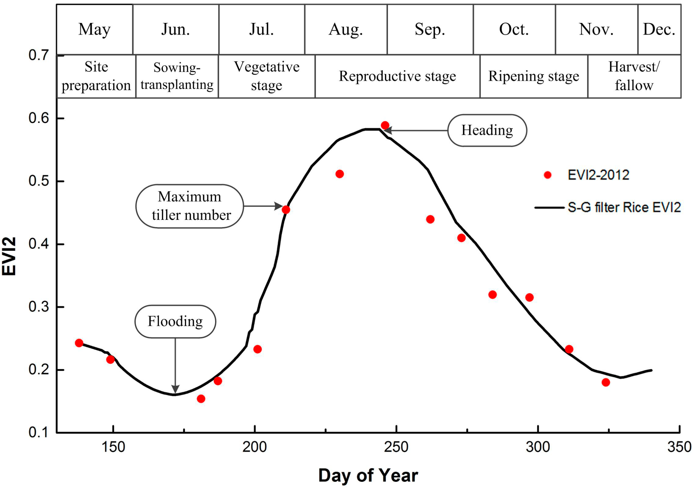
The unique physical feature of rice fields and the phenology of the SCR may provide valuable information for remote sensing classification. The rice grows on flooded soils, and the rice fields are a mixture of rice plant and open water during the transplanting and early period of the growing season [21]. As new leaves and tillers emerged, there is an accelerated increase in canopy height and leaf area of the rice. About 50 to 60 days after transplanting, the rice canopy would cover most of the surface area [22], but the leaf area is still increased till the heading stage. After that, the leaf area of rice starts to decease and the leaf color turns to yellow until the ripening and harvest stages. By using time series remote sensing images, the combined field and phenology features of rice, which differentiate the rice field from the other land cover types, may increase the classification accuracy.
To minimize the interference of external environmental factors, various vegetation indices (VIs) are commonly used in practice [23,24,25]. For example, the well-recognized normalized difference vegetation index (NDVI) [26] has been testified to be closely correlated with leaf area, biomass, percent ground cover and crop productivity [27,28,29,30]. Due to the saturation effect, however, NDVI may fail to capture the difference in well-vegetated areas, compared with the enhanced vegetation index (EVI) [31]. In practice, the time series signatures of NDVI and EVI derived from the MODIS and SPOT data had been used to map the area, species (single, early, and late), and key phenologies of rice [13,18,32]. Recently, a novel VI, i.e., the 2-band EVI (EVI2), has been proposed and testified to be comparable with the traditional EVI, and more importantly, it may achieve greater consistencies across sensors because only 2 bands are involved, as compared with 3 bands in EVI [33,34].
In addition to the data used, it is of critical importance to select appropriate classification method to properly mapping the rice fields. It is our interest to compare the classification efficiencies of the commonly used parametric and nonparametric classification algorithms, i.e., the maximum likelihood classifier (MLC) and support vector machines (SVM), with a two-step classification method proposed in this study and specifically designed to classify the rice fields from the other land cover types. The MLC is one of the most commonly used classification techniques [35,36,37]. It is a parametric classification algorithm with the assumption that the class signatures are normally distributed. The SVM is a nonparametric classifier, which projects the training data in the input space into a high dimensional space using a kernel function where the classes are linearly separable [38]. The SVMs have no limitation about the probability distribution forms of the class signature, but its performance largely depends on the kernel used, the parameter choice for the specific kernel, and the method used to generate the SVM [39,40,41].
Our study aimed to investigate the capability of EVI2 in SCR growth monitoring, and to test the feasibility of using HJ-1A/B CCD data to estimate the SCR growing area in the eastern plain region of China. For this purpose, we proposed a simple but effective classification method, which makes use of the time series HJ-1A/B imageries and the specific signatures of EVI2 (including its 1st derivative) at key phenology stages of the SCR. An extensive field campaign was carried out for verification simultaneously. We compared the effectiveness of this method with the parametric and nonparametric classification algorithms, namely MLC and SVM. We also discussed the influence of the mixed-pixel which was typical in the study area and may affect the classification accuracy.

2. Data and Methods

2.1. Study Area

Deqing County lies in the west of Hangjiahu Plain, with mean annual temperature ranging between 13 °C and 16 °C and annual precipitation of 1379 mm (Figure 1). The plain areas mainly distribute at the eastern Deqing, with the altitudes ranging from 4 m along the Beijing-Hangzhou Grand Canal to 721 m on the Tianmu Mountains. Deqing County is part of the SCR growing region in the water network area of north Zhejiang [42], where countless lakes, ponds and winding rivers scattered throughout this region, with the addition of well-developed road networks, leading to fragmented patches of irregular crop land plots. Deqing has a total area of 936 km2, and the SCR area in Deqing accounts for more than 91% of the major crop areas according to the statistical data of local agriculture department. The SCR fields mainly concentrate in the eastern regions of Deqing with average elevation less than 20 m.
Figure 1. HJ-1A CCD false-color composite image of the study area on 19 November 2012.
Remotesensing 07 03467 g001

2.2. Field Campaigns

To facilitate the remote sensing classification and verification, a continuous field campaign was carried out to record the phenologies of the SCR. Additionally, five field sites named A to E were also selected at the east of Deqing County. All the sites were larger than 1 km2, and were surveyed using a handheld GPS receiver (Trimble Juno-SB). For each land cover patch, the boundary and the corresponding land cover type were recorded. The land cover types were classified as rice, trees, water bodies, economic crops and other nonvegetated areas. The vector format maps of the five field sites in 2012 were shown in Figure 2. These maps were then reclassified into SCR and non-rice area and converted into raster format at 30 m resolution as ground-truth data for accuracy assessment.
Figure 2. Vector maps and geo-locations of the five field sites.
Remotesensing 07 03467 g002

2.3. Remote Sensing Data

HJ-1A/B data from 17 May to 5 December 2012 over the study area were collected for time-series VI analysis and downloaded from the China Center for Resources Satellite Data and Application. The sensor characteristics are presented in Table 1. Total 14 HJ-1A/B images with cloud cover less than 10% during the key phenology periods of SCR were selected for the following classification procedures (Table 2).
Table 1. Technical specification of HJ-1-A/B CCD and ZY1-02C P/MS sensors.
SatellitePayloadBand No.Spectral Range (µm)Nadir Spatial Resolution (m)Swath Width (km)Repetition Cycle (day)
HJ-1A/BMultispectral CCD camera10.43–0.5230360 (700 for two)4
20.52–0.6030
30.63–0.6930
40.76–0.9030
ZY1-02CP/MS camera10.51–0.855603–5
20.52–0.5910
30.63–0.6910
40.77–0.8910
Table 2. Dates of the selected HJ-1A/B CCD images, field campaigns, and the corresponding SCR phenology stages.
NO.SatelliteDateField Campaign DatePhenology Stage
1HJ-1B2012/05/17/Fallow
2HJ-1B2012/05/28/Site preparation
3HJ-1A2012/06/292012/06/29Sowing-transplanting
4HJ-1B2012/07/05/Vegetative stage
5HJ-1B2012/07/192012/07/20Vegetative stage (tillering)
6HJ-1A2012/07/292012/07/30Vegetative stage (maximum tiller number)
7HJ-1A2012/08/172012/08/15Reproductive stage (ear differentiation)
8HJ-1B2012/09/022012/08/31Reproductive stage (heading)
9HJ-1B2012/09/182012/09/16Reproductive stage (panicle initiation and flowering)
10HJ-1B2012/09/292012/09/25Reproductive stage
11HJ-1B2012/10/102012/10/13Ripening stage (grain filling)
12HJ-1A2012/10/232012/10/27Ripening stage (milk)
13HJ-1B2012/11/06/Ripening stage
14HJ-1A2012/11/192012/11/18Harvest/fallow
To assist the selection of training samples for classification, the Chinese Resource-1 02C satellite (ZY1-02C), which provides multispectral and panchromatic images at 10 m and 5 m spatial resolutions, respectively, was used as an auxiliary data source (Table 1). The multispectral and panchromatic images of ZY1-02C were fused to facilitate location identity in field campaigns and visual interpretation.
All the HJ 1-A/B and ZY1-02C images were geometrically corrected using the Second National Soil Survey Vector Map (scale 1:10,000), and the Root Mean Square Error (RMS error) was less than one pixel (30 m). Additionally, the radiometric calibration and atmospheric correction of the HJ 1-A/B CCD data were performed, respectively. Figure 3 showed the images of HJ-1A/B CCD and ZY1-02C of field site B at different phenology stages of the SCR.
The remote sensing classification system (five land cover types) was same as the one used in the field campaign. The training samples were randomly located and visually interpreted from the ZY1-02C fused image (5 m in spatial resolution). The class separability of the training data set was analyzed using the Jeffries-Matusita (J-M) distance metric between classes [43,44]. A larger J-M distance indicates more distinct distributions between two classes. The training data were modified if the J-M distance was close to 2 between rice and the other land cover types [45,46]. The final set of training samples were 800 pixels in total. There were 354 training pixels for rice, 92 training pixels for trees, 195 training pixels for water bodies, 76 training pixels for economic crops and 83 training pixels for other nonvegetated areas. The vector data of the 5 field sites were rasterized into 30 m resolution as ground-truth data for accuracy assessment.
Figure 3. HJ-1A/B CCD and ZY1-02C false color images of the field site B at different phenology stages of the SCR: (a) to (c) were acquired from HJ-1A/B on 29 June (sowing-transplanting stage), 29 July (vegetative stage), and 2 September (reproductive stage) 2012, respectively; and (d) ZY1-02C on 19 February 2012.
Remotesensing 07 03467 g003

2.4. Classification Methods

2.4.1. Characteristics of EVI2 Time-Series Data during SCR Growing Periods

EVI2 may achieve greater consistencies across sensors because only 2 bands are involved. EVI2 is defined as follows [33]:
E V I 2 = 2.5 × ρ n i r ρ r e d ρ n i r + 2.4 × ρ r e d + 1
where ρnir and ρred are estimated surface reflectance values for near-infrared and visible red bands (HJ-1A/B CCD bands 4 and 3, respectively).
Since there are nearly always disturbances in optical remote sensing applications caused by unfavorable atmospheric conditions and sun zenith angle changes in year around and show up as undesirable noise [47,48], noise reduction is necessary before further analysis. In this study, we used the Savitzky-Golay (S-G) filters to smooth the EVI2 time-series data. The S-G filters are suitable to smooth the irregular spacing data points, e.g., the time-series HJ-1A/B CCD data used in this study [49]. The S-G filters apply an iterative weighted moving average filter to time series data, with weighting given as a polynomial of a particular degree [50,51], which can be summarized as:
g i = n = n L n R c n f i + n n
where fi represents original value at data point i; gi is the smoothed value; n is the width of the moving window to perform filtering; nL and nR corresponding to the left and right edges of the signal component. For a specific uneven time-series data in a moving window, cn is not a constant but a polynomial fitting function, depending on the user’s preference. The fitting function can be defined as quadratic polynomial for a specific fi:
c n ( t ) = c 1 + c 2 t + c 3 t 2
where t corresponds to the day of year in EVI2 time-series.
The S-G filter was implemented using IDL 8.0 programming language to perform an image-based EVI2 time-series filtering for the HJ-1A/B CCD data from 17 May to 5 December 2012 in the study area. In this way, the time-series EVI2 curves of the five land cover types could be used to identify the most critical stages to distinguish between different land cover types.

2.4.2. Single-Cropped Rice Classification Method

In this study, we proposed a classification method which is based on the assumption that the probability distribution functions (PDFs) of the land cover types follow normal distributions [52,53]. For this purpose, we tested the samples’ probability distributions of the five land cover types using the Quantile-Quantile Plot (Q-Q Plot) [54], and it showed that normal distribution assumption was acceptable.
Using the training data set, the mean (μ) and standard deviation (σ) of each land cover type can be obtained, and then we can define the normal distribution function for each land cover type using these two parameters. To properly differentiate one specific land cover type from the others, it is crucial to minimize the overlaps between the target and the neighboring normal PDFs. For two land cover types L1 and L2, assuming L1~N(μ1, σ12) and L2~N(μ2, σ22), then the intersection between L1 and L2 should be as follows [55]:
x = σ 1 μ 2 + σ 2 μ 1 σ 1 + σ 2
where if x is out of [μ − 2σ, μ + 2σ] (hereafter μ(σ) can be μ11) or μ22) either), the two classes can be assumed distinguishable; if x is out of [μ − σ, μ + σ] but within [μ − 2σ, μ + 2σ], the two classes are mildly overlapped; if x is within [μ − σ, μ + σ], then the two classes are seriously overlapped. Generally, the two classes can be thought separable if x is out of [μ − σ, μ + σ].
Instead of using the whole growing period dataset, only key phenology stages images (during which the SCR are most differentiable from the other land cover types as explained later) were investigated in SCR field extraction. We used both of EVI2 and its 1st derivative, calculated by three consecutive images, to minimize the probability of mis-classification. For EVI2, we selected the image on 29 June 2012 (transplanting stage), whilst the spectral characteristic of the SCR was similar to water but not to the other land cover types, especially the trees. In addition, we made use of the quick change rate of EVI2, i.e., the 1st derivative of SCR during the vegetative stages (here we used the image on 29 July 2012) to gather further information to refine the classification results [56,57].

2.4.3. Parametric and Nonparametric Classification Algorithms

The MLC assumes that the class signatures are normally distributed and calculates the probabilities of a given pixel belonging to each class. The pixel is assigned to the class with the highest probability [58]. The SVM classifier is a kernel-based machine learning technique; it separates the classes with a decision surface which maximizes the margin between the classes. The success of the SVM depends on how well the process is trained. In this study, a well-known radial basis function (RBF) kernel was used in the SVM [19,38,41].
We applied the MLC and SVM using the same training samples and parameters for each classifier. The multi-temporal HJ-1 CCD data, i.e., six scenes from 2012/06/29 to 2012/09/02 during SCR transplanting to early reproductive stages, were used. The six reflectance/EVI2 imageries were composited and classified using the MLC and SVM separately, and the results were compared with the method proposed in Section 2.4.2.

2.4.4. Classification Accuracy Assessment

To assess classification accuracy, the ground-truth data (30 m resolution) were used. The ground-truth pixel numbers for field site A to E were 2842, 3078, 3186, 3248, and 2350, respectively. The proposed classification results were compared with the local agricultural statistic data in 2012. The user’s and producer’s accuracies, overall accuracy and Kappa statistic were also used to evaluate the SCR classification accuracy among the proposed method and the traditional methods, i.e., MLC and SVM.

2.5. Influence of the Mixed-Pixel

To analyze the relationship between the land cover structure (or fragmentation) and classification accuracy, we calculated the landscape metrics, i.e., class area (CA), percent of landscape (%LAND), patch density (PD), mean patch size (MPS), area-weighted mean shape index (AWMSI), and mean nearest-neighbor distance (MNN), for each ground-truth site at class level using FRAGSTATS to quantify its structure property [59]. Among the landscape metrics used here, CA is a measure of how much of the landscape is composed of a particular land cover type; %LAND is the percent of each land cover type; PD is the number of patches on a per unit area; MPS is the average area of patches for a certain class; AWMSI measures the area-weighted average patch shape; and MNN measures the mean average nearest distance among patches in a class. The landscape indices, e.g., PD, MPS, AWMSI and MNN, can be used to represent the fragmentation of land cover for a specific field site. The larger the values of PD, AWMSI and MNN, the more fragmented the site was; and vice versa for MPS.
To evaluate the influence of the land cover composition of a specific pixel on the classification accuracy, the vector maps of the five ground-truth sites were further divided into cells of size 30 m × 30 m using the gridlines derived from the HJ CCD images (only the SCR fields were kept and the other land cover types were taken as background). We calculated the area proportion of SCR in each cell, and divided the cells, in which the SCR area were greater than zero, into three grades, i.e., 75%–100%, 50%–75%, and <50%, according to the SCR area proportion. For each grade in per site, the proportion of cells, which were classified as rice field in the HJ CCD images, to the total cell number in that specific grade was calculated. We further calculated the number of misclassified pixels, i.e., the commission and omission errors, and analyzed the corresponding spatial distribution of the misclassified pixels. For a specific pixel, the commission error means that the pixel’s SCR area proportion is less than 50% but is classified as rice field; while the omission error means that the pixel contains more than 50% SCR area but is classified as the other land cover types.

3. Results

3.1. Time-Series EVI2 Characteristics

The temporal dynamics of time-series EVI2 of the SCR processed by S-G filters and the other land cover types calculated from HJ-1A/B images were shown in Figure 4 and Figure 5. The EVI2 of water bodies varied slightly over the growing season of SCR in the range of 0.07–0.14. During the transplanting and early part of the SCR growing period, rice fields were flooded and its spectral signature was similar to that of the water bodies. Not surprisingly, the EVI2 value of rice fields was very close to water bodies but obviously lower than that of trees and economic crops on June 29 (DOY = 181, about 10 days after transplanting in 2012). After transplanting, the EVI2 of SCR increased rapidly and maximized at about 0.6 between the ear differentiation and early heading stages, about 75 days after transplanting. Caused by the etiolation and senescence of the SCR leaves, the EVI2 started to decrease after the heading period till harvest.
The EVI2 values of the other nonvegetated areas, including residential areas, roads and bare land, were similar with less fluctuation but relatively higher compared with water bodies. The trees class had relatively high EVI2 values around 0.30 to 0.47. The economic crops were generally planted during a similar period as the SCR were transplanted, but usually have a longer life cycle and relativly small changing rate of EVI2 compared with SCR, especially during the vegetative stages of SCR. During the transplanting period, the water like spectral characteristic of the SCR made its EVI2 signature a little lower than the economic crops.
Figure 4. Time-series EVI2 data fitted by the S-G filters.
Remotesensing 07 03467 g004
Figure 5. Time-series EVI2 of the five land use types processed by the S-G filters.
Remotesensing 07 03467 g005

3.2. Classification Thresholds

The normal distributions of EVI2 on 29 June 2012 and its first derivative on 29 July 2012 of the five land cover types were shown in Figure 6. During the transplanting stage, the rice fields were flooded and the PDF of EVI2 of the SCR was close to that of the water bodies, and it also mixed with the nonvegetated areas and economic crops classes. Therefore, except the trees, which were mildly separable with respect to the economic crops but highly distinguishable from the other classes, the EVI2 signature of SCR was seriously overlapped with the other three land cover types (Figure 6a). Obviously, it is insufficient to identify the SCR just using images in the transplanting period.
Figure 6. Normal distributions of the five land cover types: (a) EVI2 on 29 June 2012; and (b) the 1st derivative of EVI2 on 29 July 2012.
Remotesensing 07 03467 g006
During the vegetative stages of the SCR, there was a quick increase of EVI2 due to the formation of additional tillers (Figure 4), while the increase rates of the economic crops and trees were not as steep as SCR. The other two land cover types didn’t show obvious changes during this period. In this situation, the 1st derivative of EVI2 based on the image on 29 July 2012, when the maximum tiller number had arrived, demonstrated that the rice fields could be confidently distinguished from the water bodies and the other nonvegetated areas (Figure 6b). As shown in Figure 6a, the rice fields class was distinguishable from the trees using EVI2 signatures during the transplanting stage, and it is mildly separable from the economic crops class. By using Equation (4), one pixel could be classified as rice field if its EVI2 value on 29 June 2012 equal or less than 0.24, whilst its 1st derivative of EVI2 on 29 July 2012 was equal or greater than 0.010.

3.3. Classification Accuracy Assessment

Based on the coupling thresholds of EVI2 and its 1st derivative of the SCR, during the key phenology stages, i.e., the transplanting and the vegetative to reproductive transition phases, the rice fields in Deqing County was classified using HJ-1A/B data in 2012 (Figure 7). The classified rice fields, with an area of about 94.0 km2, mainly concentrated in the eastern plain region of the study area with altitudes around 4 m. According to the statistical data of the local agriculture department in 2012, the total acreage of the SCR was 86.4 km2, so the relative classification accuracy was about 91.2%.
Figure 7. Classification result of the SCR fields using HJ-1A/B data in 2012.
Remotesensing 07 03467 g007
Table 3. Classification accuracies and Kappa coefficients of the five ground-truth sites for SCR. The last column corresponded to that if all sites were treated as a whole.
Classification AccuracyABCDEAll
Producer’s accuracy (%)95.4394.1290.7294.9895.6794.35
User’s accuracy (%)75.177.2969.1786.3183.4278.70
Overall accuracy (%)92.4390.6891.9394.2193.4091.68
Kappa coefficient0.760.750.710.850.830.79
We compared the classification accuracies of the 5 ground-truth sites (Table 3). The overall classification accuracy and Kappa coefficient for all the sites were 91.68% and 0.79, respectively. For each site, the producer’s and user’s accuracies of rice, overall classification accuracy and Kappa coefficient are listed in Table 3, in which the site D had the highest user’s accuracy and overall classification accuracy (86.31% and 94.21%, respectively), followed by site E, with user’s accuracy of 83.42% and overall accuracy of 93.40%. All the ground-truth sites had producer’s accuracies higher than 90.72% (site C). The accuracy assessment demonstrated a satisfactory result of the proposed classification method.

3.4. Comparison of Classification Methods

The classification accuracy of the proposed method used in this study outperformed the MLCs and SVMs (Table 4 and Table 5). By using EVI2 instead of the reflectance data, the MLC-EVI2 and SVM-EVI2 improved the classification accuracies to certain extent, but not significant, compared with their counterparts, respectively. The MLCs and SVMs also showed better classification accuracies in site D and site E. While site C had a lower classification result compared with the other four field sites.
Table 4. Classification accuracies and Kappa coefficients of the five ground-truth sites for SCR using MLC and SVM methods. The last column is the corresponding results if all sites were treated as a whole.
Classification MethodsClassification AccuracyABCDEAll
MLC-EVI2Producer’s accuracy (%)67.7770.7760.6877.0170.6962.41
User’s accuracy (%)67.0863.8361.4373.2573.6860.58
Overall accuracy (%)88.8585.1084.0389.1787.8184.88
Kappa coefficient0.710.680.680.600.740.65
MLC-ReflectanceProducer’s accuracy (%)68.6066.4852.9779.9370.2762.55
User’s accuracy (%)65.2361.2156.1569.4970.2757.52
Overall accuracy (%)88.4283.7481.5488.5886.7283.83
Kappa coefficient0.700.630.640.700.720.65
SVM-EVI2Producer’s accuracy (%)82.2383.3860.0583.7681.0773.97
User’s accuracy (%)50.9052.4350.9059.1461.1654.33
Overall accuracy (%)83.4680.1776.9685.3785.3481.09
Kappa coefficient0.630.620.570.550.690.61
SVM-ReflectanceProducer’s accuracy (%)84.3085.8260.9685.4079.1074.80
User’s accuracy (%)50.0051.6351.5158.4063.8752.87
Overall accuracy (%)82.9778.2376.3584.7884.2780.00
Kappa coefficient0.630.590.560.550.610.57
Table 5. Landscape indices of the five land cover types in the ground-truth sites.
SiteClassCA (ha)%LANDPDMPS (ha)AWMSIMNN (m)
ARice50.0825.781.560.641.7327.41
Trees44.9923.162.200.452.8319.45
Water bodies69.1235.581.220.822.5418.03
Economic crops2.321.196.890.151.40126.17
Other nonvegetated areas27.7714.294.830.217.7630.91
BRice60.8530.251.250.802.1121.90
Trees56.7328.201.730.583.2321.38
Water bodies48.1223.921.410.713.8620.32
Economic crops3.751.865.330.195.6780.80
Other nonvegetated areas31.7215.774.480.224.5517.64
CRice40.5019.661.310.761.5722.14
Trees45.4722.071.830.552.5615.98
Water bodies74.0835.950.901.112.1020.15
Economic crops7.553.672.250.441.3492.04
Other nonvegetated areas38.4418.664.630.227.3421.30
DRice70.3136.030.951.051.2513.85
Trees32.1216.461.960.512.2013.24
Water bodies62.6132.081.150.871.947.00
Economic crops5.953.0515.120.074.3821.55
Other nonvegetated areas24.1512.388.490.1218.5313.50
ERice55.6231.151.110.901.4013.64
Trees41.6323.322.450.411.9714.60
Water bodies43.7424.500.781.292.6022.36
Economic crops5.883.295.440.181.5865.06
Other nonvegetated areas31.6717.745.270.198.2919.73

3.5. Influence of the Mixed-Pixel

In the five ground-truth sites (Table 5), the average area percentage of water bodies was the highest among the 5 land cover types (larger than 0.71 in five field sites), followed by rice and trees (larger than 0.64 and 0.41, respectively). About 36.03% area of site D was rice, compared with the smallest proportion of 19.66% in site C. The site D had the smallest trees area proportion of 16.46%. The economic crops had the smallest area, and its average patch size in site D was only 0.07 ha, smaller than the area of one pixel of HJ-1 CCD image (30 m × 30 m); the high values of MNN also indicated the highly scattered status of the economic crops (see also Figure 2), and economic crops had the largest value of MNN of the five categories for five field sites. The other nonvegetated areas had the highest AWMSI (except site B), reflecting the complex shape of the road system. The fragmentation statuses of rice, indicated by PD, AWMSI and MNN, of sites D and E were the lowest compared with sites AC; while the site D and E had the highest MPS. The sites D and E had less fragmented degrees compared with site C, while sites A and B had intermediate level of fragmentation statuses of rice.
Figure 8 showed the ratios of the pixels which were classified as rice field in the HJ CCD images to the total pixel number (ground-truth data, pixels in which the area proportion of rice field is greater than 50%) in each grade for sites AE. It is obvious that the recognition ratio increased as the area proportion of rice field in pixel ascending, i.e., the grade 75%–100% had the highest classification accuracy. The site D and E had the highest recognition ratio in each grade, while site C the lowest. This result also demonstrated the difficulties in classification in fragmented areas where the mixed-pixel problems were more serious.
More than 69.03% commission pixels concentrated at the boundaries, while at least 63.89% omission pixels lay on the boundaries; that is, most of the misclassified pixels concentrated at the boundaries of the rice fields (Table 6 and Figure 9). The omission pixel numbers of sites DE were 40 and 36 respectively, obviously less than sites AC (65, 70 and 80 respectively). The misclassification error was largely determined by the commission error. As shown in Figure 9, the commission error pixels (red color) were more than the omission ones (blue color).
Figure 8. Recognition ratios for the ground-truth sites A–E, compared with the classification results of HJ CCD images.
Remotesensing 07 03467 g008
Table 6. Statistics of the pixel numbers in classification for sites A–E. The boundary pixels are the pixels which contain certain area of rice field and interface with the other land cover types; the commission pixels represent pixels in which the rice field area proportion is less than <50%, but is misclassified as rice field; and the omission pixels are pixels in which the rice field area proportion is great than 50% but is wrongly classified as the other land cover types.
Statistics of ClassificationABCDE
Rice pixel number779995678942742
Boundary pixel number476594433542369
Commission pixel number150217155144119
Commission pixels on boundary12216910710191
Omission pixel number6570804436
Omission pixels on boundary4757534023
Classification error(%) 127.6028.8434.6619.9620.89
Note: 1 The classification error is calculated as (omission number + commission number)/rice pixel number.
Figure 9. Spatial distribution of the misclassified pixels in sites (AE).
Remotesensing 07 03467 g009aRemotesensing 07 03467 g009b

4. Discussion

It is generally acknowledged that using a single-temporal image to well discriminate a specific kind of crop at various phenology stages from the other vegetation (or land cover types) is an enormous challenge [19,60,61]. However, using the spectral characteristics (or vegetation indices) determined by the key phenologies of a specific crop species, i.e., multi-temporal remote sensing imageries, is a promising way to improve the classification accuracy [62,63]. To effectively discriminate the rice field in eastern plain region of China, where the rice field is generally fragmented and irregular due to the topography and widely distributed water bodies and road networks, a specifically designed stepwise remote sensing classification strategy was applied in this study.
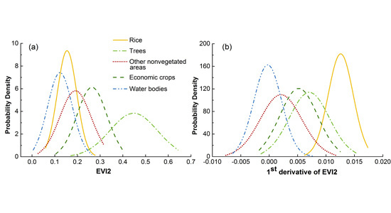
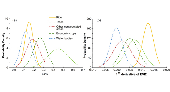
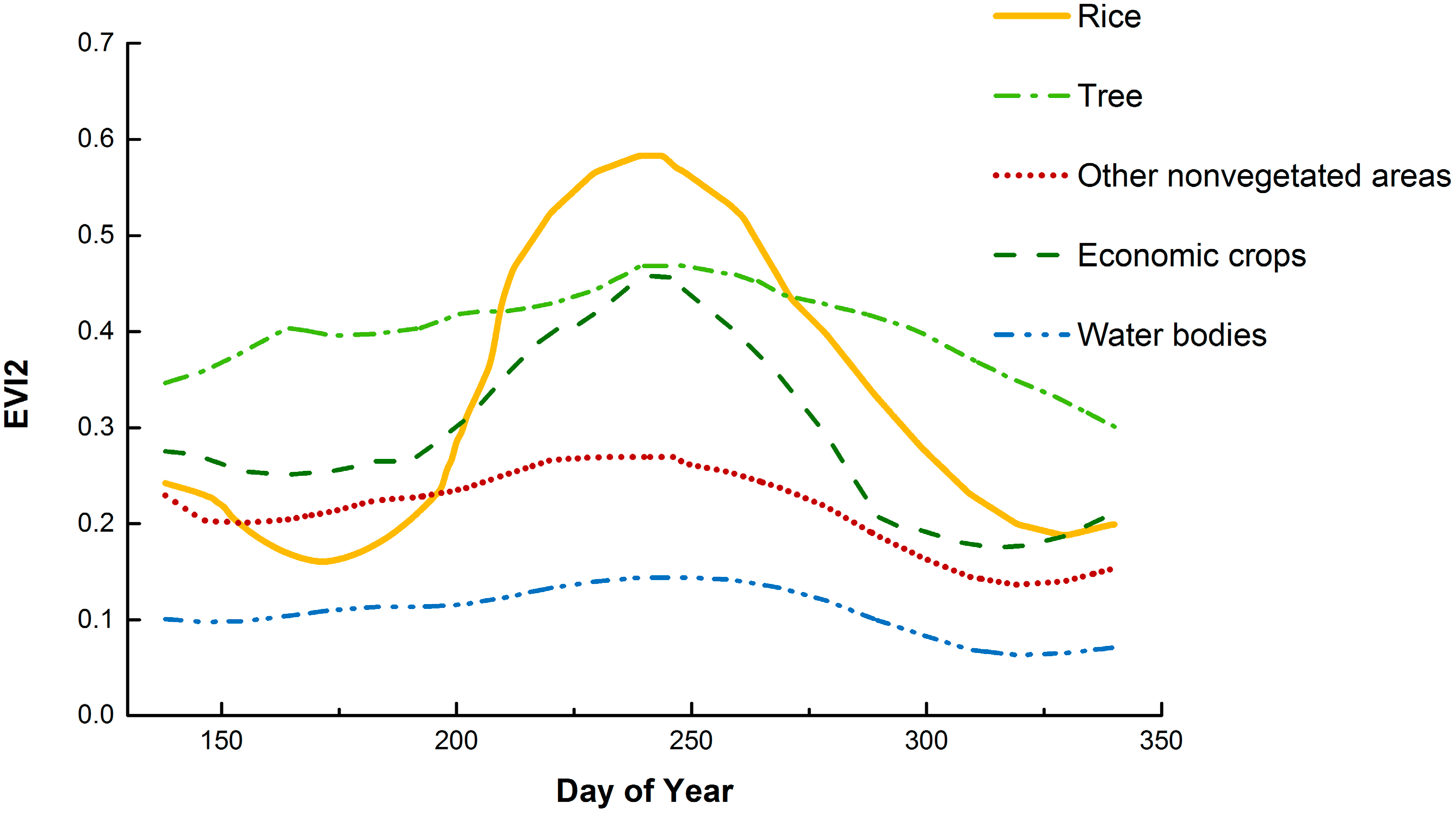
The time-series EVI2 data for the major land cover types in the study area were built from the HJ-1 A/B CCD imageries and the S-G filters was applied to smooth the EVI2 time-series. With the reference field campaign data, the EVI2 showed efficient discriminating capability in capturing the spectral differences between SCR and the other land cover types during the key SCR phenology stages (Figure 5). It is prominent that the EVI2 of SCR increased rapidly during the transplanting and ear differentiation (including early heading) stages, and the temporal resolution of HJ-1 A/B CCD data was testified to be suitable to capture these features. The stepwise classification algorithm proposed in this study can be seen as an exemplar of the decision tree classification category, and it outperformed the parametric (MLC) and nonparametric (SVM) classification algorithms, respectively (Table 3 and Table 4). By using EVI2 instead of the reflectance data, the classification accuracies improved to certain extents for both of MLC and SVM. The results also implied that by treating the satellite-derived vegetation classification information hierarchically, the mixtures among spectral feature spaces can be effectively alleviated. For MLC and SVM, total six scenes during SCR transplanting to early reproductive stages (from 2012/06/29 to 2012/09/02) were used, including the transplanting, vegetative to reproductive transition phases. However, it is noteworthy that time-series EVI2 of SCR during this period increased rapidly and intersected with the EVI2s of all the other land cover types, except water bodies (Figure 5). Therefore, the classification accuracies of MLC and SVM should unavoidably be decreased, because both of the methods treated the spectral signatures contained in the six scenes collectively.
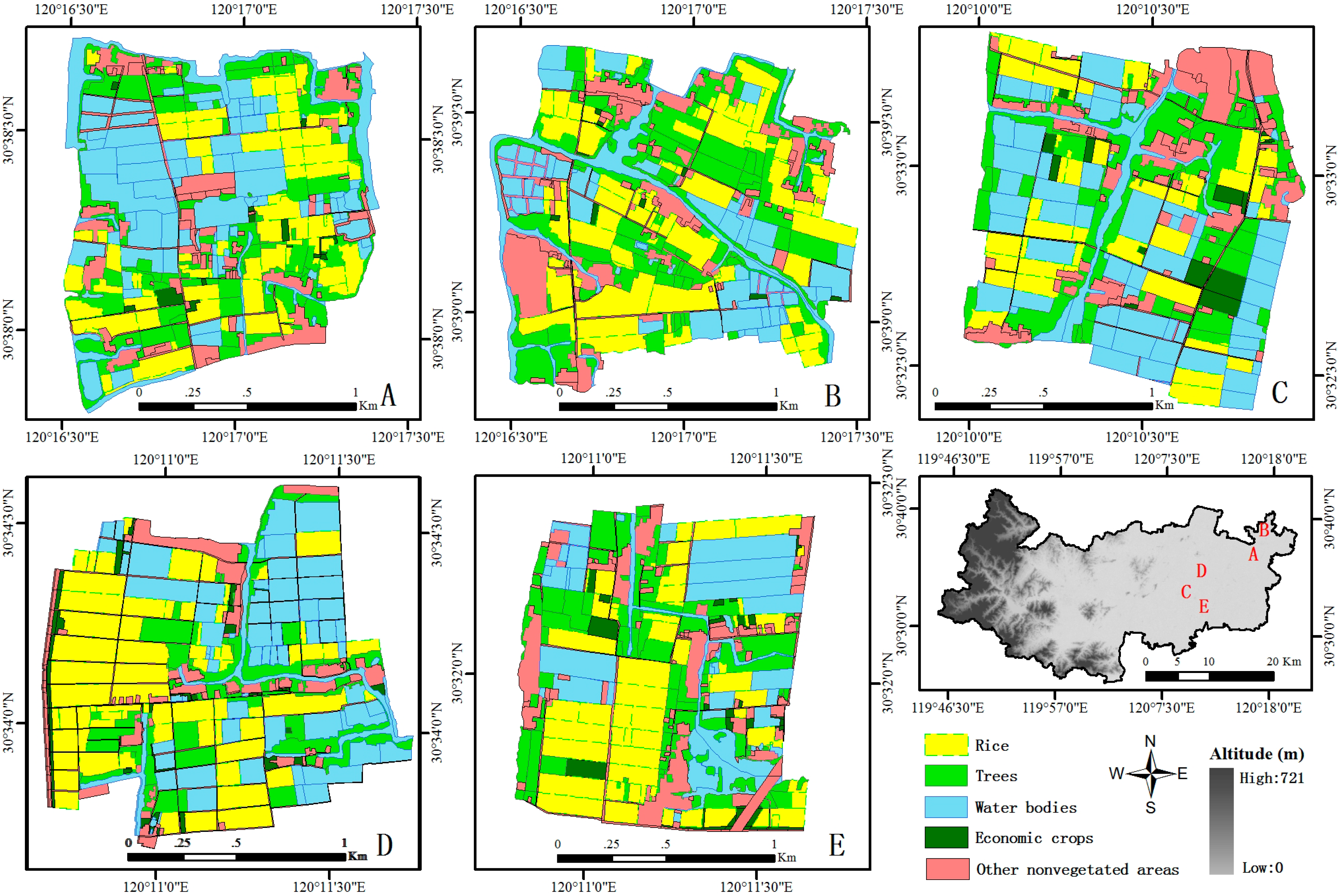
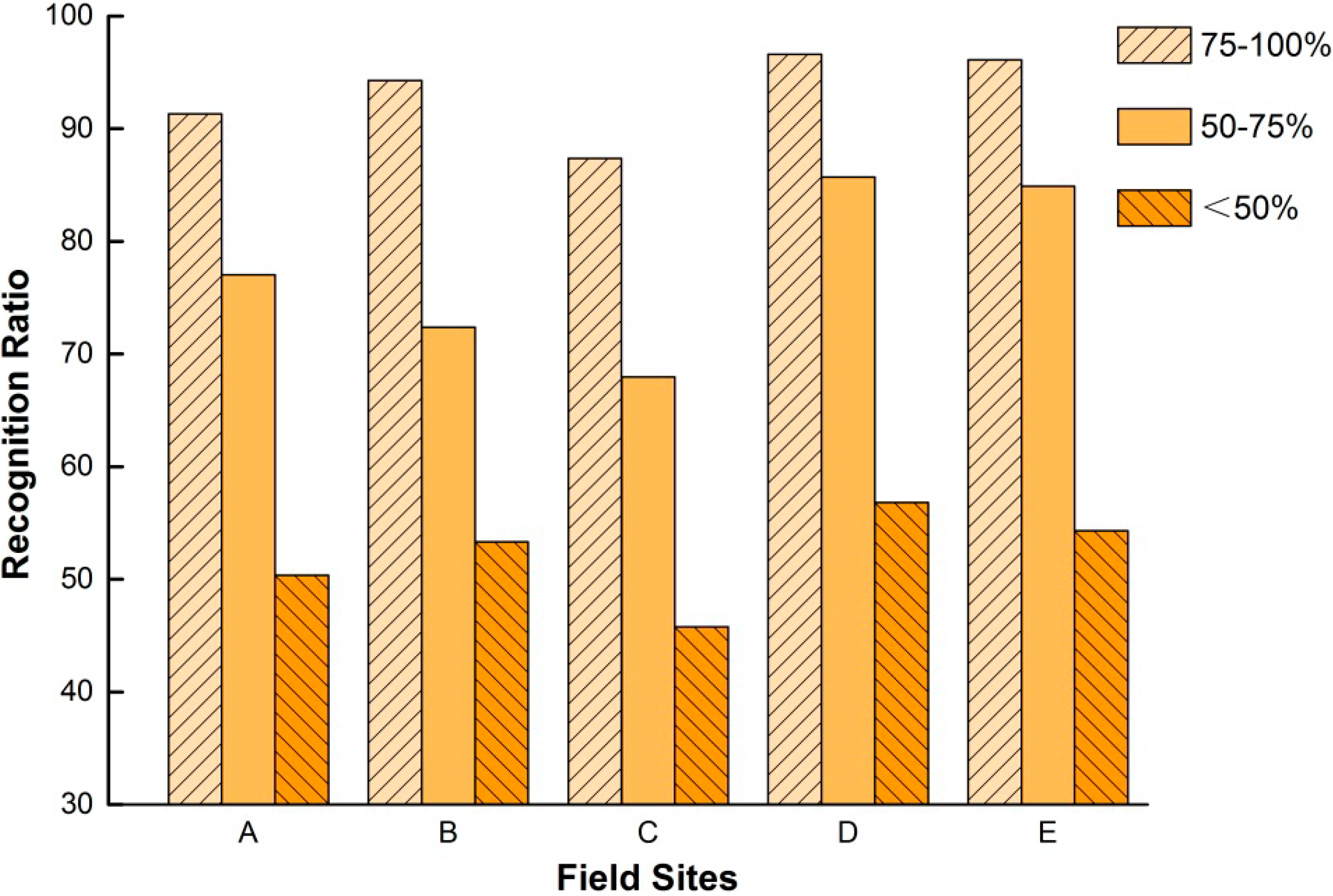
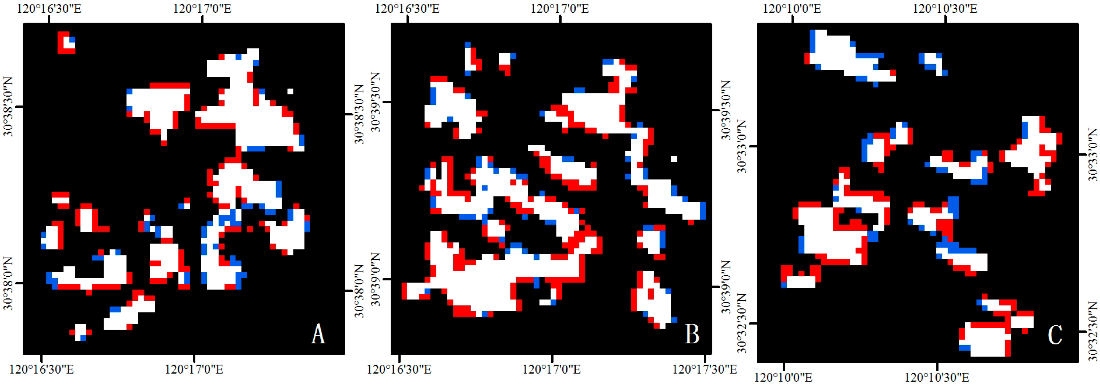
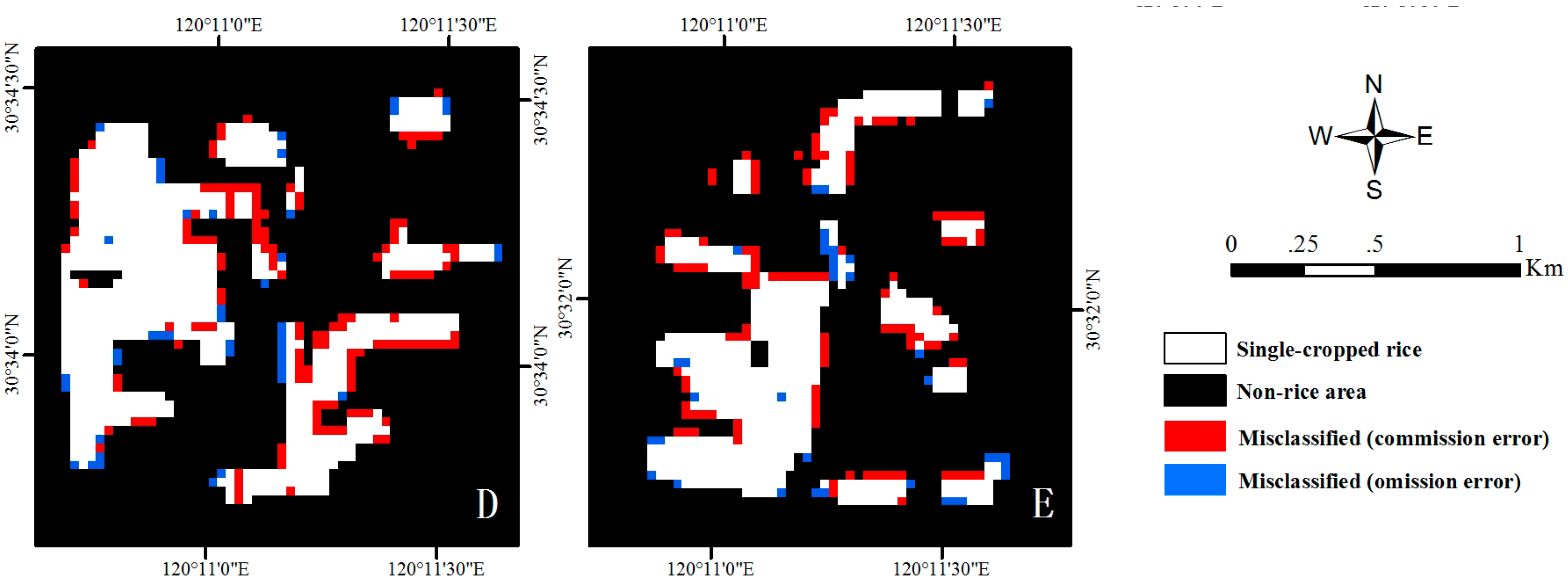
The influence of the mixed-pixel is a primary concern in remote sensing classification practices. We used five ground-truth sites as an example and analyzed the relationship between the purity of pixels (measured as the area proportion of rice field in a specific cell) and the corresponding recognition ratios. The mixed-pixel analysis showed that the recognition ratio was positively correlated with the rice field area proportion at each ground-truth site (Table 5 and Figure 8). The sites D and E showed the best recognition ratio of SCR among the five ground-truth sites, and it is in accordance with the fragmentation statuses indicated by the landscape indices (Table 5). It is not unexpectedly that as the area proportion of rice field increased in each cell, the possibility of misclassification decreased consequently, especially for the grade of 75%–100% (refer in particular to rice field).
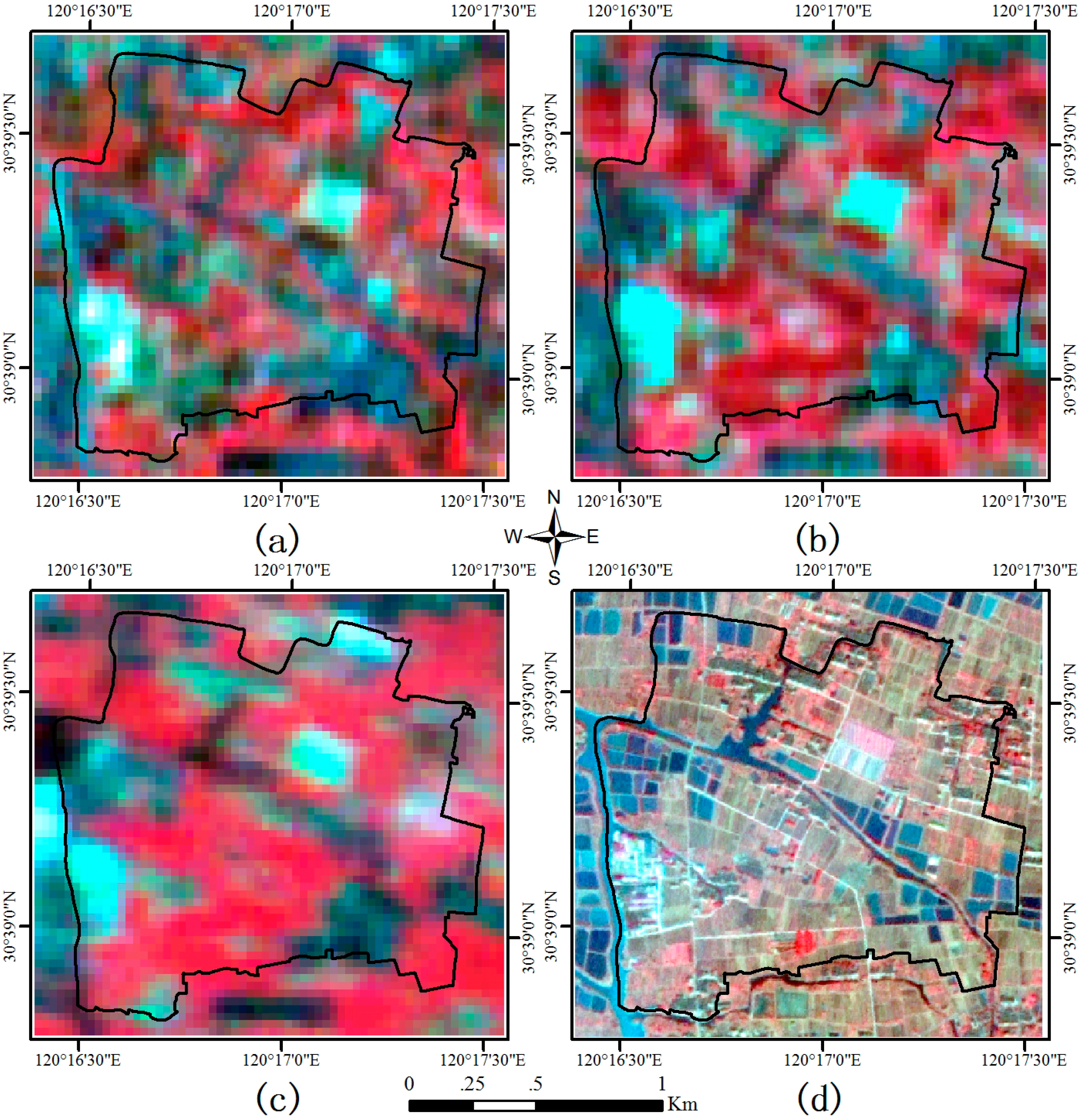
As large part of the classification error can be attributed to the influence of mixed-pixels where the area proportion of rice field was less than 75%, and most of the mixed-pixels concentrated at the boundaries of the rice fields (Table 6 and Figure 9). We further analyzed the classification error caused by the commission and omission errors due to the mixed-pixels and boundary effects, respectively. The results showed that the ratio of the edge pixels to the total rice pixel number correlated with the fragmentation states of each site, i.e., the number of the edge pixel was positively correlated with land fragmentation states of each site due to the increased rice field perimeter. As a consequence, the classification errors of sites DE were less than sites AC as shown in Table 6. For rice fields, the misclassification caused by the commission errors was more common, compared with the omission errors (i.e., cells in which rice field area was less than 50% but was classified as rice field, see Figure 8).
However, it should be noted that due to the existence of spatial autocorrelation, the classification accuracy reported in this study may be overestimated [64]. Spatial autocorrelation might be present due to large pixel size [65] or points sampled in close proximity [66]. To avoid the artificially increased classification accuracy caused by the random cross-validation using autocorrelated dataset, more than one permanent training/test dataset should be utilized in accuracy assessment [64]. In this study, five ground-truth sites with different land cover percentages were selected for classification accuracy assessment, however the authors acknowledged that the autocorrelation may still unavoidable and quantitative evaluation of its influence is still a challenge. Further studies should be focused on field data collection, with subsampling and cross-validation like k-fold method [64] to improve the classification accuracy assessment.
The extrapolation of the findings in this study must be cautious due to various changes in the environmental factors (e.g., dry or wet) and vegetation status in different regions and years. The aim of this study was to provide a general methodology in the classification of single-cropped rice. However, when applying it to another region or year, the VI thresholds, which are used to distinguish different land cover types, must be decided according to the specific time series satellite images, i.e., the VI thresholds and the timestamps (according to the key phenologies) are variable.

5. Conclusions

In this study, we applied a simple but robust stepwise algorithm to estimate the single cropped rice (SCR) growing area in irregular and fragmented regions. The multi-temporal HJ-1A/B images and specific signatures of EVI2 at the key phenology stages, i.e., the transplanting and the vegetative to reproductive transition phases, of the SCR were used to classify the rice fields from the other land use types with satisfactory results, compared with the traditional MLC and SVM methods. Due to the fragmented land use composition in the study area, we also assessed the influence of mixed-pixel quantified by using the landscape indices and it showed that the classification accuracy ratio of rice field was positively correlated with its compactness. We showed that by making full use of the key phenological information, and under the support of high-temporal resolution remote sensing data, e.g., HJ-1A/B, the SCR can be mapped at a relative high confidence. The crucial point in the proposed method was the construction of high-quality time-series VI curves, which were then used to identify the key phenology stages to differentiate different land cover types. However, due to the variation of environmental factors and the corresponding changes of vegetation status, due care should be taken when extrapolating the results to other regions or periods. Additionally, we noted that the influence of spatial autocorrelation should also be taken into consideration in classification accuracy evaluation in further study.

Acknowledgements

This research was funded by The National High Technology Research and Development Program of China (Grant No. 2012AA12A30703) and Agricultural Project of Scientific and Technological Research of Shanghai, China (2011-2-11). We are grateful to the lab members Qiaoli Ge, Sujuan Wang, Jingjing Shi, Liwen Zhang, Qiaoying Guo, Zhuokun Pan, Zhewen Zhao, Yao Zhang, Weijiao Huang, Chen Wei, Dilong Gan, Zhen Zhou, Yuanyuan Chen, Bing Han, Mengting Jin, Xiaoqiang Zhang, Jingbo Zhu, and Ran Huang for their great assistance during the field campaigns and data processing. We would also like to express our sincere thanks to the anonymous reviewers for their constructive comments.

Author Contributions

Jing Wang had the original idea for the study and wrote the original manuscript. Jingfeng Huang supervised the process of field campaign and data analysis. Kangyu Zhang provided partial source codes for image analysis. Xinxing Li was responsible for image data collection. Bao She, Chuanwen Wei and Jian Gao processed field campaign data. Xiaodong Song offered valuable comments to the manuscript and was responsible to manuscript revisions. All authors read and approved the final manuscript.

Conflicts of Interest

The authors declare no conflict of interest.

References

  1. Gnanamanickam, S.S. Rice and its importance to human life. In Rice and Its Importance to Human Life; Springer: Berlin, Germany, 2009; pp. 1–11. [Google Scholar]
  2. Gon, H.D. Changes in CH4 emission from rice fields from 1960 to 1990s: 1. Impacts of modern rice technology. Glob. Biogeochem. Cycles 2000, 14, 61–72. [Google Scholar] [CrossRef]
  3. Zhang, W.; Yu, Y.Q.; Huang, Y.; Li, T.T.; Wang, P. Modeling methane emissions from irrigated rice cultivation in China from 1960 to 2050. Glob. Change Biol. 2011, 17, 3511–3523. [Google Scholar] [CrossRef]
  4. FAOSTAT. Statistical Database of the Food and Agricultural Organization of the United Nations. Available online: http://faostat.fao.org/default.aspx?lang=en (accessed on 30 December 2014).
  5. Zhai, H. Prospects for grain demand and supply in the 21st century. In Proceedings of the 12th Toyota Conference: Challenge of Plant and Agricultural Sciences to the Crisis of the Biosphere on the Earth in the 21st Century, Shizuoka, Japan, 25–28 November 1998; pp. 29–37.
  6. Chen, C.F.; Huang, S.W.; Son, N.T.; Chang, L.Y. Mapping double-cropped irrigated rice fields in Taiwan using time-series Satellite Pour I’Observation de la Terre data. J. Appl. Remote Sens. 2011, 5. [Google Scholar] [CrossRef]
  7. Xiao, X.M.; Boles, S.; Frolking, S.; Li, C.S.; Babu, J.Y.; Salas, W.; Moore, B., III. Mapping paddy rice agriculture in South and Southeast Asia using multi-temporal MODIS images. Remote Sens. Environ. 2006, 100, 95–113. [Google Scholar] [CrossRef]
  8. Fang, H.L.; Wu, B.F.; Liu, H.Y.; Huang, X. Using NOAA AVHRR and Landsat TM to estimate rice area year-by-year. Int. J. Remote Sens. 1998, 19, 521–525. [Google Scholar] [CrossRef]
  9. Gumma, M.K.; Thenkabail, P.S.; Hideto, F.; Nelson, A.; Dheeravath, V.; Busia, D.; Rala, A. Mapping irrigated areas of Ghana using fusion of 30 m and 250 m resolution remote-sensing data. Remote Sens. 2011, 3, 816–835. [Google Scholar] [CrossRef]
  10. Yu, L.; Wang, J.; Clinton, N.; Xin, Q.C.; Zhong, L.H.; Chen, Y.L.; Gong, P. FROM-GC: 30 m global cropland extent derived through multisource data integration. Int. J. Digit. Earth 2013, 6, 521–533. [Google Scholar] [CrossRef]
  11. Kamthonkiat, D.; Honda, K.; Turral, H.; Tripathi, N.K.; Wuwongse, V. Discrimination of irrigated and rainfed rice in a tropical agricultural system using SPOT VEGETATION NDVI and rainfall data. Int. J. Remote Sens. 2005, 26, 2527–2547. [Google Scholar] [CrossRef]
  12. Sakamoto, T.; Van Nguyen, N.; Ohno, H.; Ishitsuka, N.; Yokozawa, M. Spatio–temporal distribution of rice phenology and cropping systems in the Mekong Delta with special reference to the seasonal water flow of the Mekong and Bassac Rivers. Remote Sens. Environ. 2006, 100, 1–16. [Google Scholar] [CrossRef]
  13. Sun, H.S.; Huang, J.F.; Huete, A.R.; Peng, D.L.; Zhang, F. Mapping paddy rice with multi-date moderate-resolution imaging spectroradiometer (MODIS) data in China. J. Zhejiang Univ-Sc. A. 2009, 10, 1509–1522. [Google Scholar] [CrossRef]
  14. Carfagna, E.; Gallego, F.J. Using remote sensing for agricultural statistics. Int. Stat. Rev. 2005, 73, 389–404. [Google Scholar] [CrossRef]
  15. Wu, B.F.; Li, Q.Z. Crop planting and type proportion method for crop acreage estimation of complex agricultural landscapes. Int. J. Appl. Earth Obs. 2012, 16, 101–112. [Google Scholar] [CrossRef]
  16. Asner, G.P. Cloud cover in Landsat observations of the Brazilian Amazon. Int. J. Remote Sens. 2001, 22, 3855–3862. [Google Scholar] [CrossRef]
  17. Pyongsop, R.I.; Zhangbao, M.A.; Qingwen, Q.I.; Gaohuan, L. Cloud and shadow removal from Landsat TM data. J. Remote Sens. 2010, 14, 534–545. [Google Scholar]
  18. Chen, J.S.; Huang, J.X.; Hu, J.X. Mapping rice planting areas in southern China using the China Environment Satellite data. Math. Comput. Model. 2011, 54, 1037–1043. [Google Scholar] [CrossRef]
  19. Jia, K.; Wu, B.F.; Li, Q.Z. Crop classification using HJ satellite multispectral data in the North China Plain. J. Appl. Remote Sens. 2013, 7. [Google Scholar] [CrossRef]
  20. Li, W.G.; Li, H.; Zhao, L.H. Estimating Rice Yield by HJ-1A Satellite Images. Rice Sci. 2011, 18, 142–147. [Google Scholar] [CrossRef]
  21. Xiao, X.M.; Boles, S.; Frolking, S.; Salas, W.; Moore, B., III; Li, C.; He, L.; Zhao, R. Observation of flooding and rice transplanting of paddy rice fields at the site to landscape scales in China using VEGETATION sensor data. Int. J. Remote Sens. 2002, 23, 3009–3022. [Google Scholar] [CrossRef]
  22. Le Toan, T.; Ribbes, F.; Wang, L.F.; Floury, N.; Ding, K.H.; Kong, J.A.; Fujita, M.; Kurosu, T. Rice crop mapping and monitoring using ERS-1 data based on experiment and modeling results. IEEE Trans. Geosci. Remote Sens. 1997, 35, 41–56. [Google Scholar] [CrossRef]
  23. Baret, F.; Guyot, G. Potentials and limits of vegetation indices for LAI and APAR assessment. Remote Sens. Environ. 1991, 35, 161–173. [Google Scholar] [CrossRef]
  24. Gitelson, A.A. Remote estimation of crop fractional vegetation cover: the use of noise equivalent as an indicator of performance of vegetation indices. Int. J. Remote Sens. 2013, 34, 6054–6066. [Google Scholar] [CrossRef]
  25. Meng, J.H.; Wu, B.F.; Chen, X.Y.; Du, X.; Niu, L.M.; Zhang, F.F. Validation of HJ-1 B charge-coupled device vegetation index products with spectral reflectance of Hyperion. Int. J. Remote Sens. 2011, 32, 9051–9070. [Google Scholar] [CrossRef]
  26. Rouse, J.W.; Haas, R.H.; Schell, J.A.; Deering, D.W.; Harlan, J.C. Monitoring the Vernal Advancement and Retrogradation of Natural Vegetation; NASA/GSFC, Type III, Final Report; Texas AM University: College Station, TX, USA, 1974. [Google Scholar]
  27. De Rosnay, P.; Calvet, J.-C.; Kerr, Y.; Wigneron, J.-P.; Lemaître, F.; Escorihuela, M.J.; Sabater, J.M.; Saleh, K.; Barrié, J.; Bouhours, G. SMOSREX: A long term field campaign experiment for soil moisture and land surface processes remote sensing. Remote Sens. Environ. 2006, 102, 377–389. [Google Scholar] [CrossRef]
  28. Gao, S.; Niu, Z.; Huang, N.; Hou, X. Estimating the Leaf Area Index, height and biomass of maize using HJ-1 and RADARSAT-2. Int. J. Appl. Earth Obs. 2013, 24, 1–8. [Google Scholar] [CrossRef]
  29. Hansen, P.M.; Schjoerring, J.K. Reflectance measurement of canopy biomass and nitrogen status in wheat crops using normalized difference vegetation indices and partial least squares regression. Remote Sens. Environ. 2003, 86, 542–553. [Google Scholar] [CrossRef]
  30. Lu, L.; Li, X.; Huang, C.L.; Ma, M.G.; Che, T.; Bogaert, J.; Veroustraete, F.; Dong, Q.H.; Ceulemans, R. Investigating the relationship between ground-measured LAI and vegetation indices in an alpine meadow, north-west China. Int. J. Remote Sens. 2005, 26, 4471–4484. [Google Scholar] [CrossRef]
  31. Huete, A.; Didan, K.; Miura, T.; Rodriguez, E.P.; Gao, X.; Ferreira, L.G. Overview of the radiometric and biophysical performance of the MODIS vegetation indices. Remote Sens. Environ. 2002, 83, 195–213. [Google Scholar] [CrossRef]
  32. Xiao, X.M.; Boles, S.; Liu, J.Y.; Zhuang, D.F.; Frolking, S.; Li, C.S.; Salas, W.; Moore, B., III. Mapping paddy rice agriculture in southern China using multi-temporal MODIS images. Remote Sens. Environ. 2005, 95, 480–492. [Google Scholar] [CrossRef]
  33. Jiang, Z.Y.; Huete, A.R.; Didan, K.; Miura, T. Development of a two-band enhanced vegetation index without a blue band. Remote Sens. Environ. 2008, 112, 3833–3845. [Google Scholar] [CrossRef]
  34. Kim, Y.; Miura, T.; Jiang, Z.; Huete, A.R. Spectral compatibility of vegetation indices across sensors: band decomposition analysis with Hyperion data. J. Appl. Remote Sens. 2010, 4. [Google Scholar] [CrossRef]
  35. DeFries, R.S.; Townshend, J. NDVI-derived land cover classifications on a global scale. Int. J. Remote Sens. 1994, 15, 3567–3586. [Google Scholar] [CrossRef]
  36. Hubert-Moy, L.; Cotonnec, A.; Le Du, L.; Chardin, A.; Perez, P. A comparison of parametric classification procedures of remotely sensed data applied on different landscape units. Remote Sens. Environ. 2001, 75, 174–187. [Google Scholar] [CrossRef]
  37. Yang, C.H.; Everitt, J.H.; Murden, D. Evaluating high resolution SPOT 5 satellite imagery for crop identification. Comput. Electron. Agr. 2011, 75, 347–354. [Google Scholar] [CrossRef]
  38. Chen, C.F.; Son, N.T.; Chen, C.R.; Chang, L.Y. Wavelet filtering of time-series moderate resolution imaging spectroradiometer data for rice crop mapping using support vector machines and maximum likelihood classifier. J. Appl. Remote Sens. 2011, 5. [Google Scholar] [CrossRef]
  39. Foody, G.M.; Mathur, A. Toward intelligent training of supervised image classifications: directing training data acquisition for SVM classification. Remote Sens. Environ. 2004, 93, 107–117. [Google Scholar] [CrossRef]
  40. Mountrakis, G.; Im, J.; Ogole, C. Support vector machines in remote sensing: A review. ISPRS J. Photogramm. Remote Sens. 2011, 66, 247–259. [Google Scholar] [CrossRef]
  41. Rao, T.V. Supervised classification of remote sensed data using support vector machine. Glob. J. Comput. Sci. Technol. 2014, 14, 71–76. [Google Scholar]
  42. Xu, H.W.; Wang, K. Regionalization for rice yield estimation by remote sensing in Zhejiang Province. Pedosphere 2001, 11, 175–184. [Google Scholar]
  43. Lobo, A.; Chic, O.; Casterad, A. Classification of Mediterranean crops with multisensor data: per-pixel versus per-object statistics and image segmentation. Int. J. Remote Sens. 1996, 17, 2385–2400. [Google Scholar] [CrossRef]
  44. Panigrahy, S.; Parihar, J.S.; Patel, N.K. Kharif rice acreage estimation in Orissa using NOAA-AVHRR data. J. Indian Soc. Remote Sens. 1992, 20, 35–42. [Google Scholar] [CrossRef]
  45. Congalton, R.G. A Review of Assessing the Accuracy of Classifications of Remotely Sensed Data. Remote Sens. Environ. 1991, 37, 35–46. [Google Scholar] [CrossRef]
  46. Wardlow, B.D.; Egbert, S.L.; Kastens, J.H. Analysis of time-series MODIS 250 m vegetation index data for crop classification in the US Central Great Plains. Remote Sens. Environ. 2007, 108, 290–310. [Google Scholar] [CrossRef]
  47. Pan, Z.; Huang, J.; Zhou, Q.; Wang, L.; Cheng, Y.; Zhang, H.; Blackburn, G.A.; Yan, J.; Liu, J. Mapping crop phenology using NDVI time-series derived from HJ-1 A/B data. Int. J. Appl. Earth Obs. 2015, 34, 188–197. [Google Scholar] [CrossRef]
  48. Sakamoto, T.; Wardlow, B.D.; Gitelson, A.A.; Verma, S.B.; Suyker, A.E.; Arkebauer, T.J. A Two-Step Filtering approach for detecting maize and soybean phenology with time-series MODIS data. Remote Sens. Environ. 2010, 114, 2146–2159. [Google Scholar] [CrossRef]
  49. Cong, N.; Piao, S.; Chen, A.; Wang, X.; Lin, X.; Chen, S.; Han, S.; Zhou, G.; Zhang, X. Spring vegetation green-up date in China inferred from SPOT NDVI data: A multiple model analysis. Agr. Forest Meteorol. 2012, 165, 104–113. [Google Scholar] [CrossRef]
  50. Hird, J.N.; McDermid, G.J. Noise reduction of NDVI time series: An empirical comparison of selected techniques. Remote Sens. Environ. 2009, 113, 248–258. [Google Scholar] [CrossRef]
  51. Jönsson, P.; Eklundh, L. TIMESAT—A program for analyzing time-series of satellite sensor data. Comput. Geosci. 2004, 30, 833–845. [Google Scholar] [CrossRef]
  52. Li, A.N.; Jiang, J.G.; Bian, J.H.; Deng, W. Combining the matter element model with the associated function of probability transformation for multi-source remote sensing data classification in mountainous regions. ISPRS J. Photogramm. Remote Sens. 2012, 67, 80–92. [Google Scholar] [CrossRef]
  53. Voisin, A.; Krylov, V.A.; Moser, G.; Serpico, S.B.; Zerubia, J. Supervised classification of multisensor and multiresolution remote sensing images with a hierarchical copula-based approach. IEEE Trans. Geosci. Remote Sens. 2013, 52, 3346–3358. [Google Scholar] [CrossRef]
  54. Zhang, D.X.; Zhang, C.R.; Li, W.D.; Cromley, R.; Hanink, D.; Civco, D.; Travis, D. Restoration of the missing pixel information caused by contrails in multispectral remotely sensed imagery. J. Appl. Remote Sens. 2014, 8. [Google Scholar] [CrossRef]
  55. Hu, L.H.; Yu, Z.F.; Liu, Y.F. An algorithm of decision-tree generating automatically based on classification. In Proceedings of the First International Workshop on Education Technology and Computer Science, Wuhan, China, 7–8 March 2009; Vol. I, pp. 823–827.
  56. Jonsson, P.; Eklundh, L. Seasonality extraction by function fitting to time-series of satellite sensor data. IEEE Trans. Geosci. Remote Sens. 2002, 40, 1824–1832. [Google Scholar] [CrossRef]
  57. Sakamoto, T.; Yokozawa, M.; Toritani, H.; Shibayama, M.; Ishitsuka, N.; Ohno, H. A crop phenology detection method using time-series MODIS data. Remote Sens. Environ. 2005, 96, 366–374. [Google Scholar] [CrossRef]
  58. Otukei, J.R.; Blaschke, T. Land cover change assessment using decision trees, support vector machines and maximum likelihood classification algorithms. Int. J. Appl. Earth Obs. 2010, 12S, S27–S31. [Google Scholar] [CrossRef]
  59. Li, X.; Lu, L.; Cheng, G.D.; Xiao, H.L. Quantifying landscape structure of the Heihe River Basin, north-west China using FRAGSTATS. J. Arid Environ. 2001, 48, 521–535. [Google Scholar] [CrossRef]
  60. Murthy, C.S.; Raju, P.V.; Badrinath, K. Classification of wheat crop with multi-temporal images: performance of maximum likelihood and artificial neural networks. Int. J. Remote Sens. 2003, 24, 4871–4890. [Google Scholar] [CrossRef]
  61. Shao, Y.; Fan, X.T.; Liu, H.; Xiao, J.H.; Ross, S.; Brisco, B.; Brown, R.; Staples, G. Rice monitoring and production estimation using multitemporal RADARSAT. Remote Sens. Environ. 2001, 76, 310–325. [Google Scholar] [CrossRef]
  62. Han, H.B.; Ma, M.B.; Wang, X.F.; Ma, S.C. Classifying cropping area of middle Heihe River Basin in China using multitemporal Normalized Difference Vegetation Index data. J. Appl. Remote Sens. 2014, 8. [Google Scholar] [CrossRef]
  63. Nuarsa, I.W.; Nishio, F.; Hongo, C.; Mahardika, I.G. Using variance analysis of multitemporal MODIS images for rice field mapping in Bali Province, Indonesia. Int. J. Remote Sens. 2012, 33, 5402–5417. [Google Scholar] [CrossRef]
  64. Mannel, S.; Price, M.; Hua, D. Impact of reference datasets and autocorrelation on classification accuracy. Int. J. Remote Sens. 2011, 32, 5321–5330. [Google Scholar] [CrossRef]
  65. Friedl, M.A.; Woodcock, C.; Gopal, S.; Muchoney, D.; Strahler, A.H.; Barker-Schaaf, C. A note on procedures used for accuracy assessment in land cover maps derived from AVHRR data. Int. J. Remote Sens. 2000, 21, 1073–1077. [Google Scholar] [CrossRef]
  66. Mannel, S.; Price, M.; Hua, D. A method to obtain large quantities of reference data. Int. J. Remote Sens. 2006, 27, 623–627. [Google Scholar] [CrossRef]

