
Monitoring of Evapotranspiration in a Semi-Arid Inland River Basin by Combining Microwave and Optical Remote Sensing Observations


Abstract
:
1. Introduction
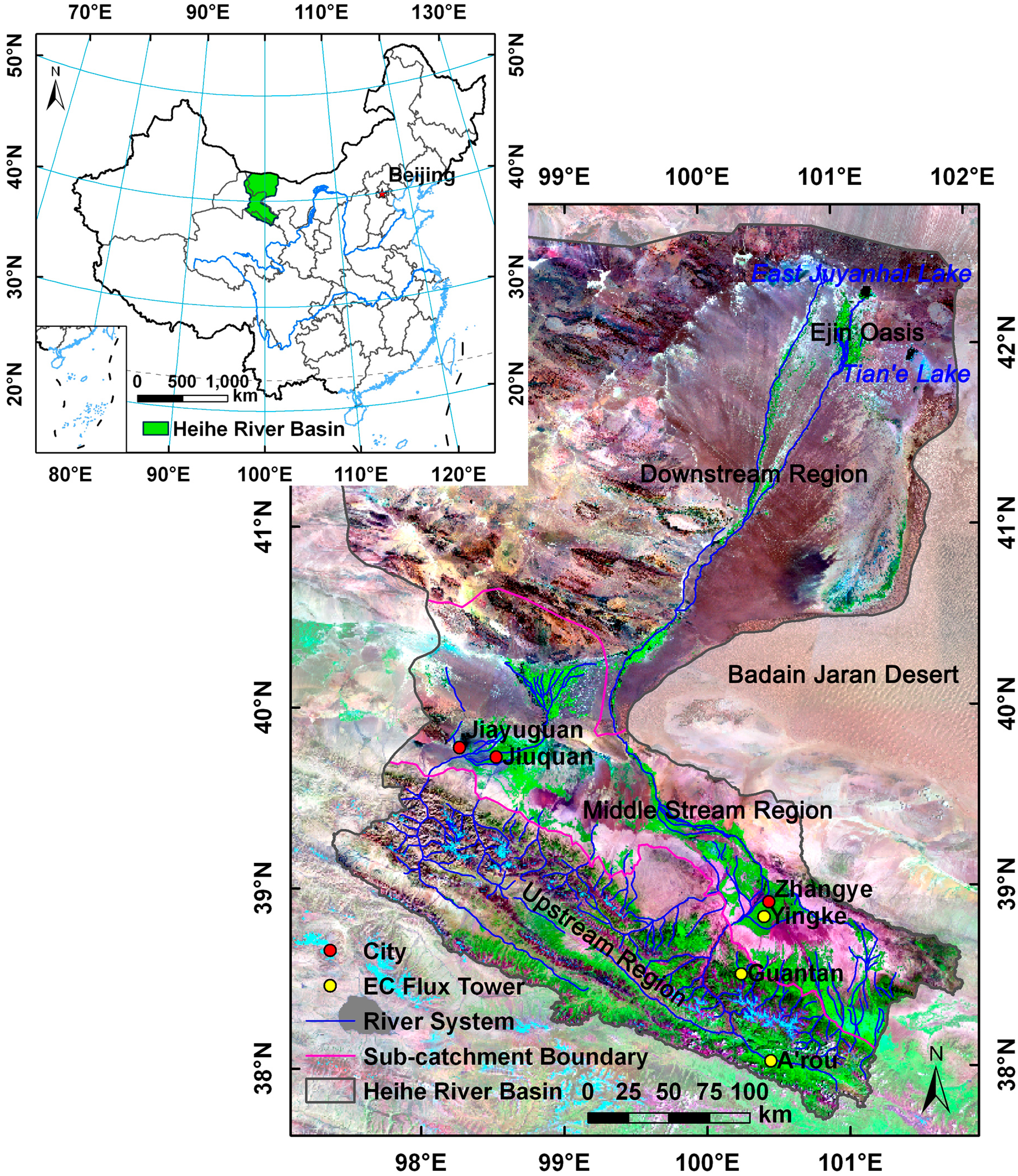
2. Study Area

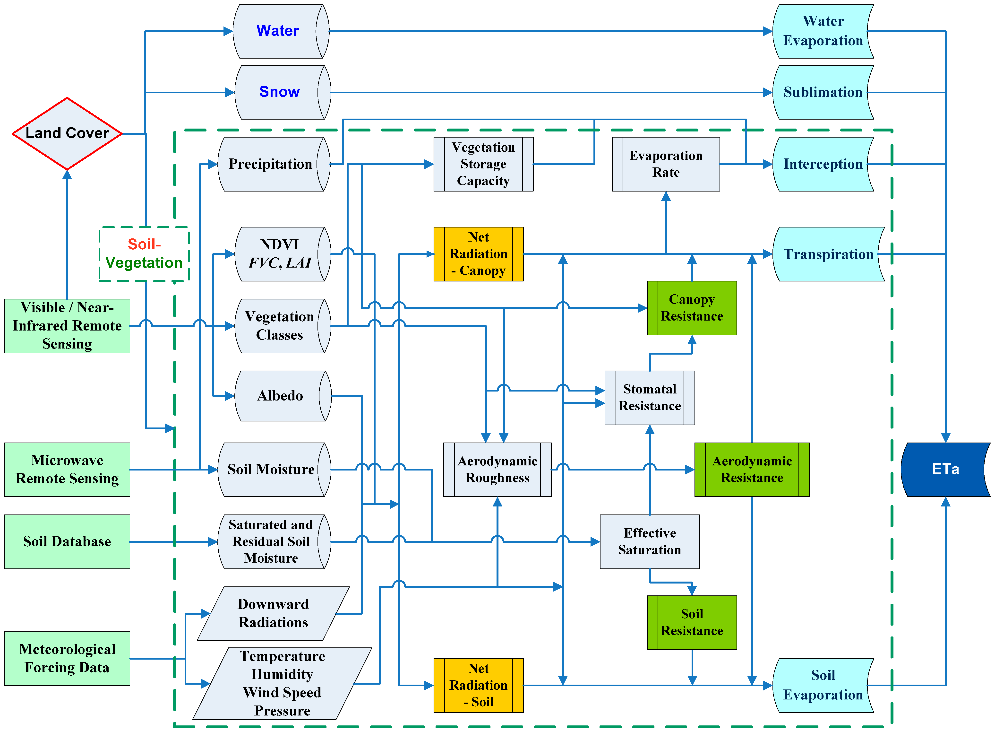
3. Theoretical Formulation of the ETMonitor Model

3.1. Evapotranspiration of the Soil–Vegetation Unity
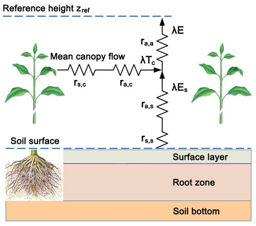
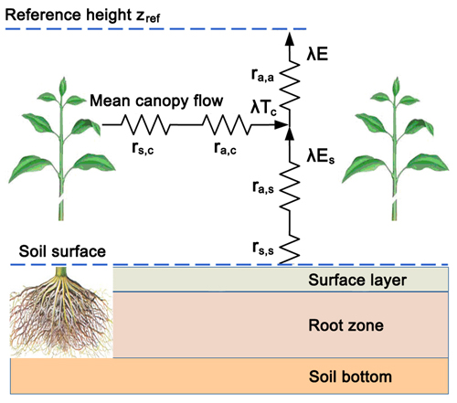
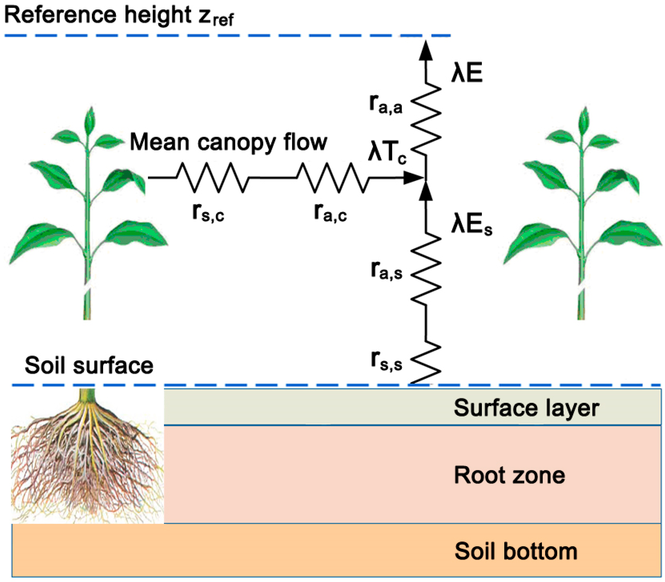
3.1.1. Shuttleworth–Wallace Dual-Source Model

3.1.2. Resistances
(1) Aerodynamic Resistance
(2) Soil Surface Resistance
(3) Canopy Surface Resistance
3.2. Interception
3.3. Sublimation
3.4. Evaporation from Water Surface
4. Data
4.1. Remote Sensing Data
4.1.1. Land Surface Albedo
4.1.2. Normalized Difference Vegetation Index (NDVI)
4.1.3. Soil Moisture
4.1.4. Land Cover
4.1.5. Snow Cover Extent
4.1.6. Precipitation
4.2. Soil Texture and Hydraulic Parameters
4.3. Meteorological Forcing Data
4.4. Eddy Covariance Flux Data

| Site Name | Sensors | Location/Elevation | Landscape | Data DOI |
|---|---|---|---|---|
| Yingke | CSAT3 (Campbell) and Li7500 (Li-cor) | 100°24′37.2″E | Cropland (maize) | 10.3972/water973.0278.db |
| 38°51′25.7″N | ||||
| 1519.1 m | ||||
| A’rou | 100°27′52.9″E | Alpine Meadow | 10.3972/water973.0282.db | |
| 38°02′39.8″N | ||||
| 3032.8 m | ||||
| Guantan | 100°15′00.8″E | Spruce Forest | 10.3972/water973.0294.db | |
| 38°32′01.3″N | ||||
| 2835.2 m |
4.5. MOD16 ETa
5. Results
5.1. Validation of the Model
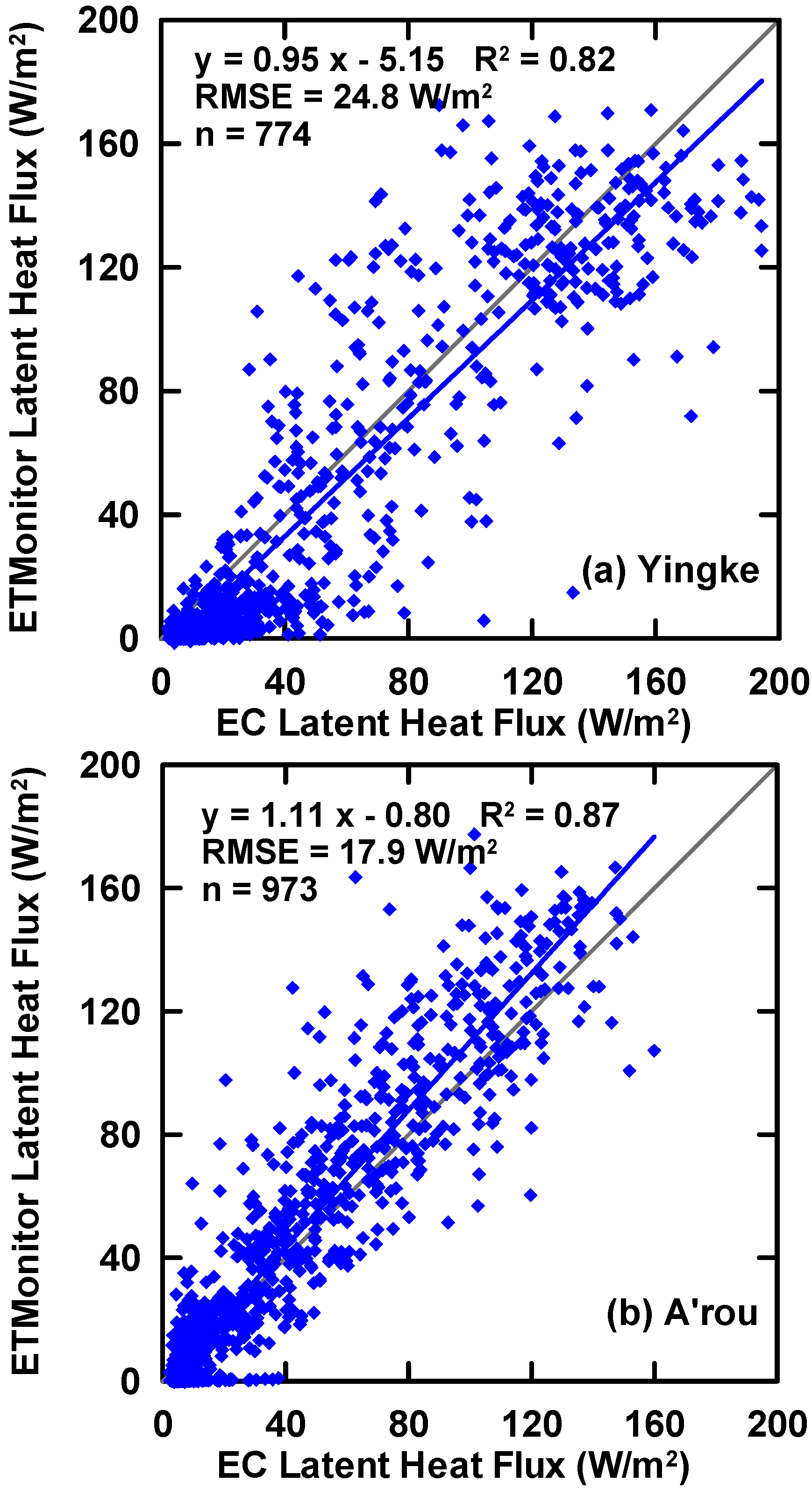
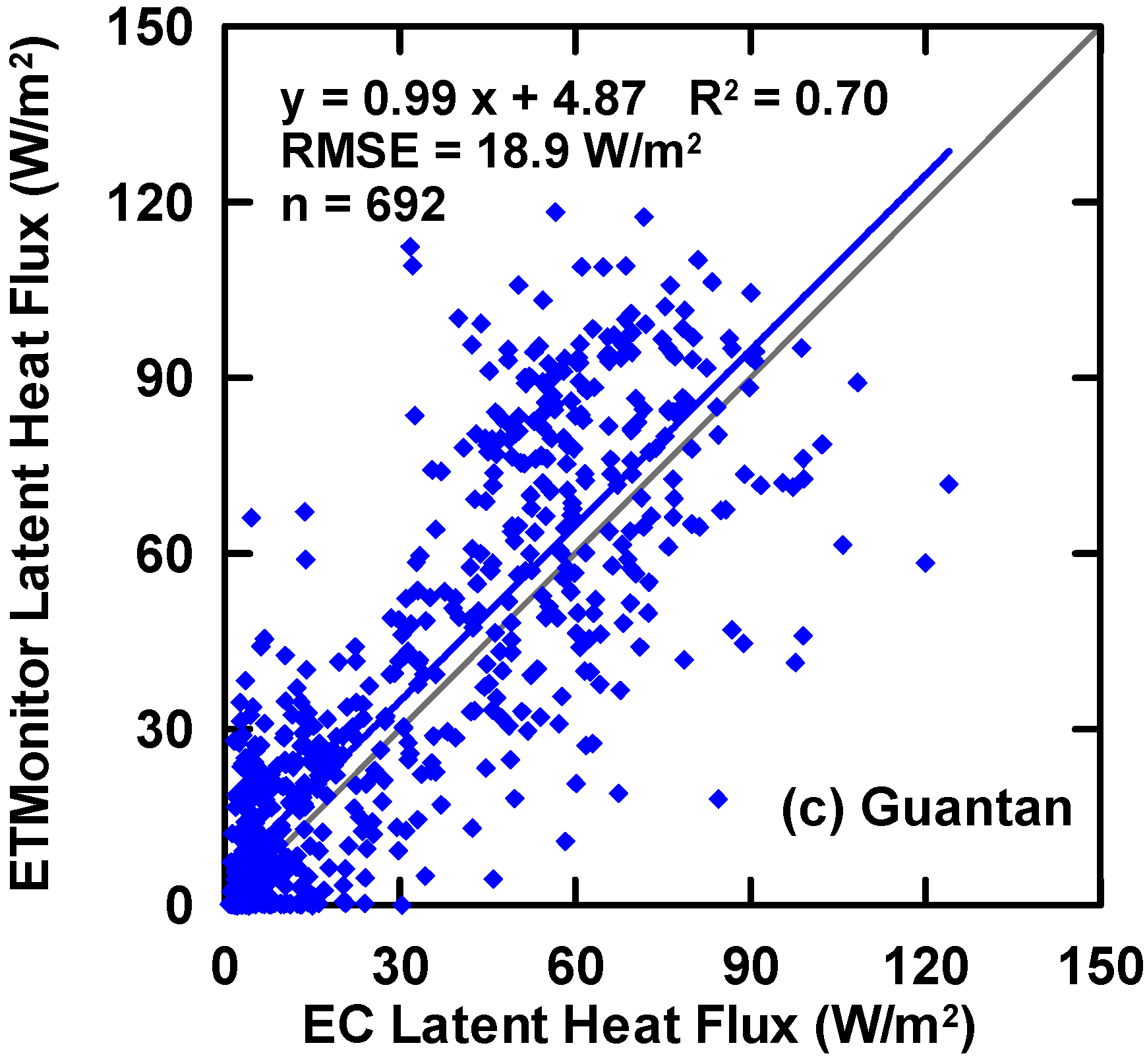
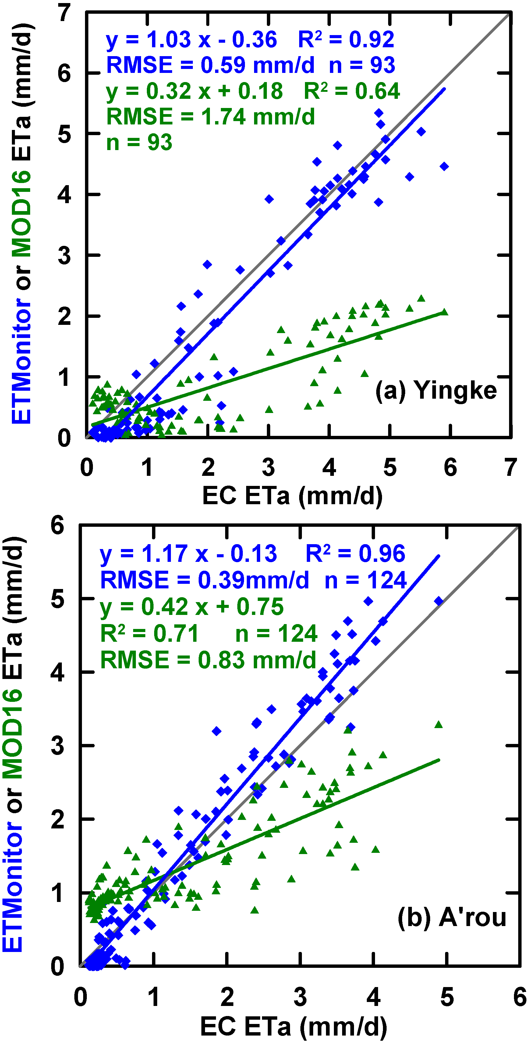
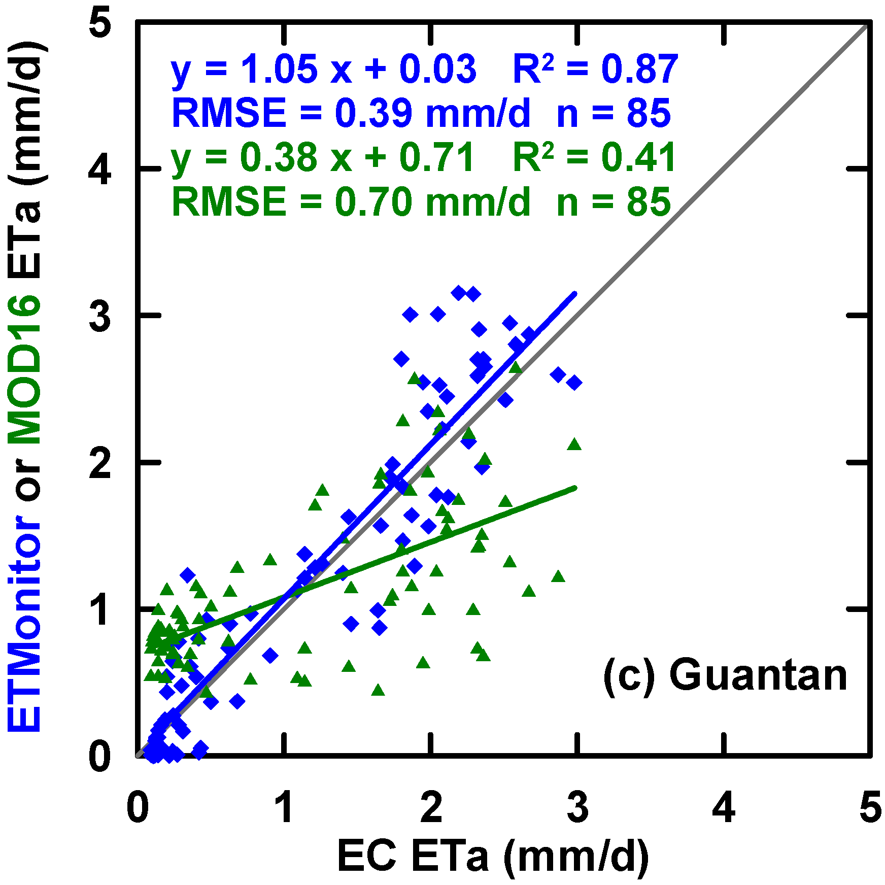
5.1.1. Comparison with the Ground Measurements


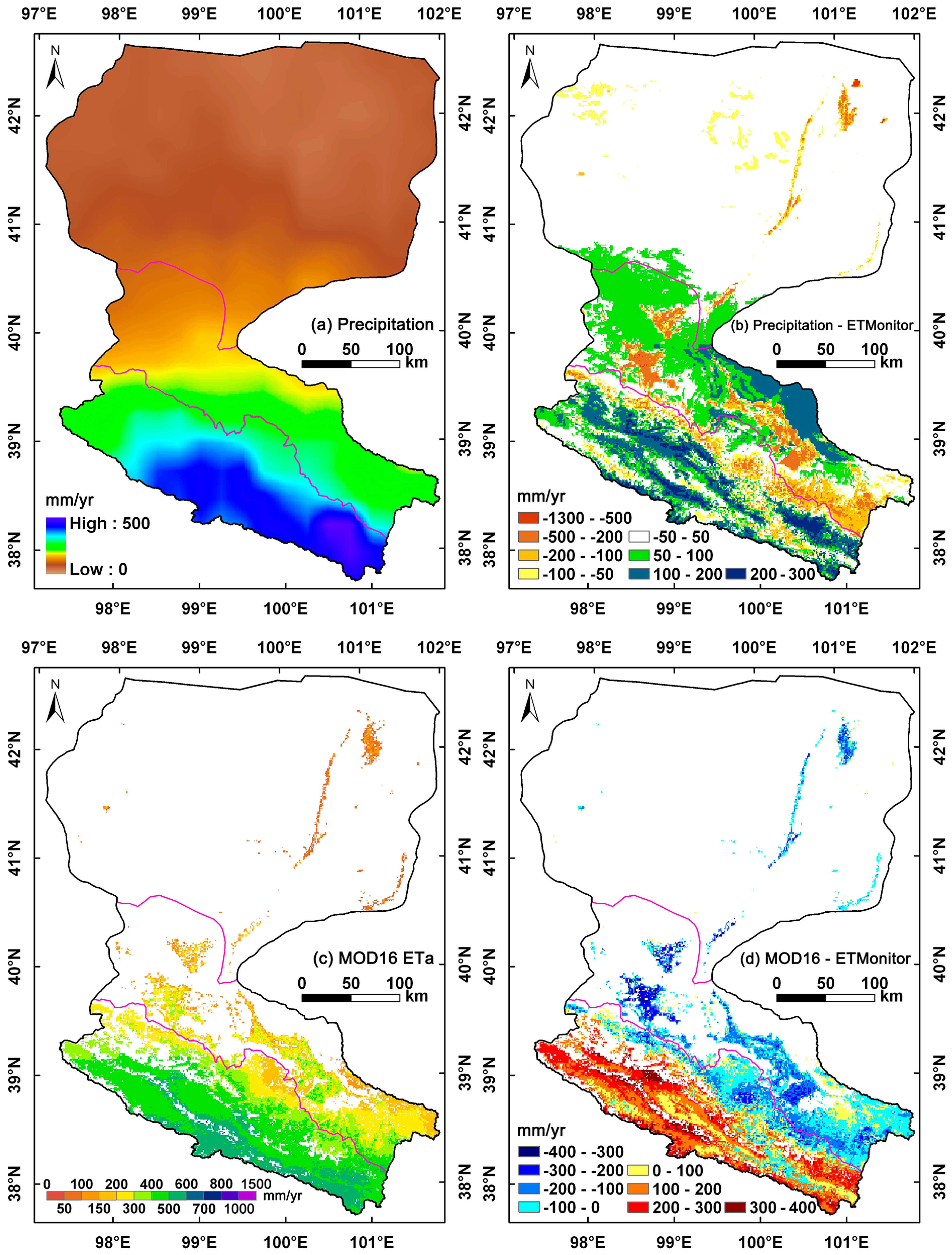
5.1.2. Spatial Intercomparison with Precipitation and MOD16 ETa


5.2. Sensitivity Analysis

| Parameter | Reference Value | ETr (mm·d−1) | ET0.9r (mm·d−1) | ET1.1r (mm·d−1) | Sensitivity | |
|---|---|---|---|---|---|---|
| NDVI | NDVI (-) | 0.66 | 3.562 | 2.914 | 3.964 | 0.295 |
| Albedo | Albedo (-) | 0.19 | 3.619 | 3.505 | 0.032 | |
| Surface layer soil water content | θg (cm3·cm−3) | 0.12 | 3.373 | 3.748 | 0.105 | |
| Air temperature | Ta (°C) | 21.3 | 3.365 | 3.662 | 0.084 | |
| Air pressure | P (Pa) | 84540 | 3.877 | 3.287 | 0.166 | |
| Specific humidity | Q (kg·kg−1) | 0.006 | 3.605 | 3.514 | 0.026 | |
| Wind speed | u (m·s−1) | 3 | 3.570 | 3.564 | 0.002 | |
| Downward short-wave radiation | Rs (W·m−2) | 293.8 | 3.193 | 3.932 | 0.207 | |
| Downward long-wave radiation | Rl (W·m−2) | 330.8 | 3.230 | 3.893 | 0.186 | |
| Minimum stomatal resistance | rst,min (s·m−1) | 180 | 3.744 | 3.398 | 0.097 | |
| Minimum soil surface resistance | rs,s,min (s·m−1) | 50 | 3.601 | 3.528 | 0.021 | |
| Saturated soil water content | θsat (cm3·cm−3) | 0.5 | 3.768 | 3.390 | 0.106 | |
| Solar radiation factor | kRs (W·m−2) | 500 | 3.693 | 3.440 | 0.071 | |
| Optimum air temperature | Topt (°C) | 25 | 3.595 | 3.510 | 0.024 | |
| Vapor pressure deficit factor | kVPD (hPa−1) | 0.023 | 3.671 | 3.446 | 0.063 | |
| Tenacity factor | Ksf (-) | 1.5 | 3.402 | 3.709 | 0.086 | |
5.3. ETa Spatial and Temporal Variations in the Heihe River Basin
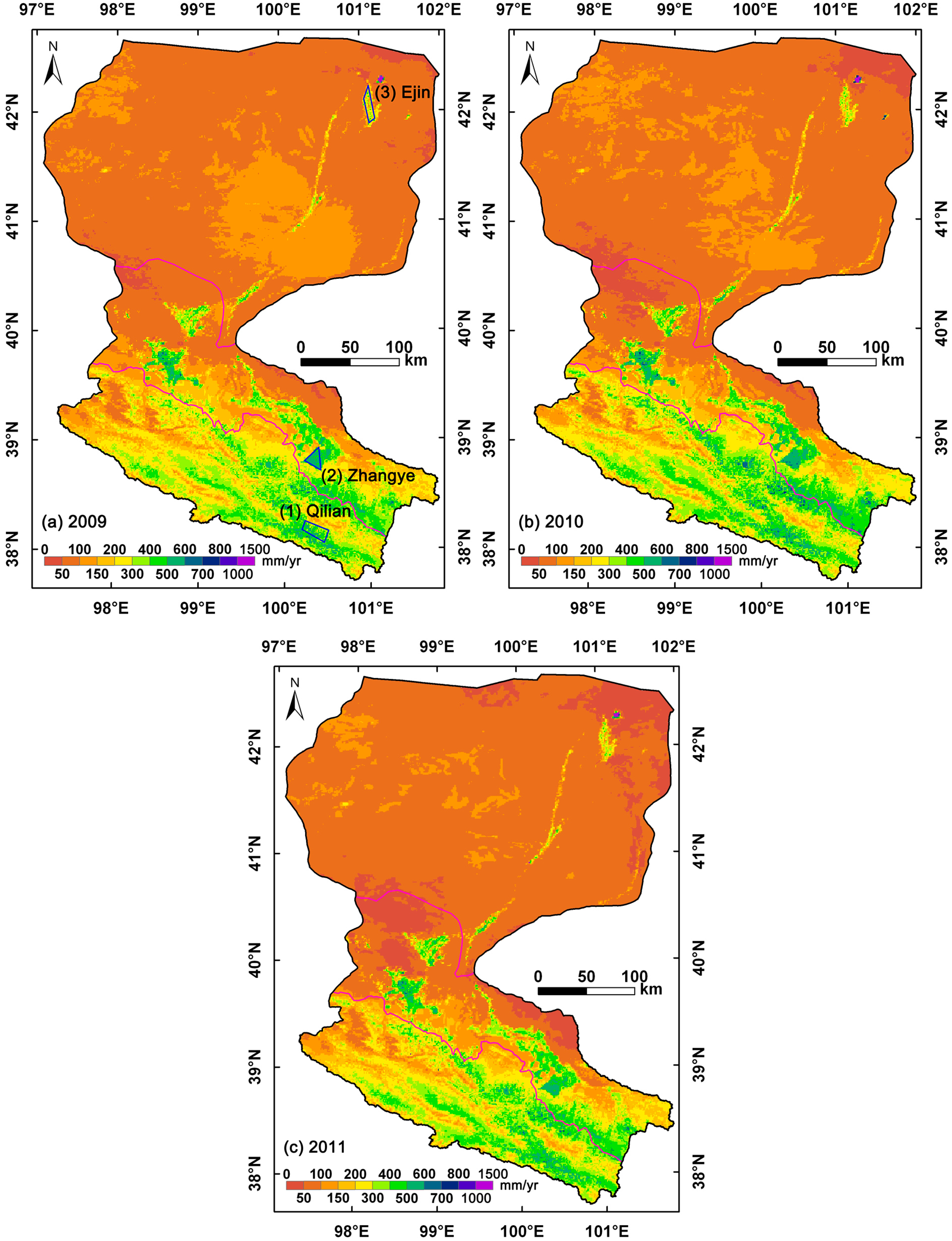
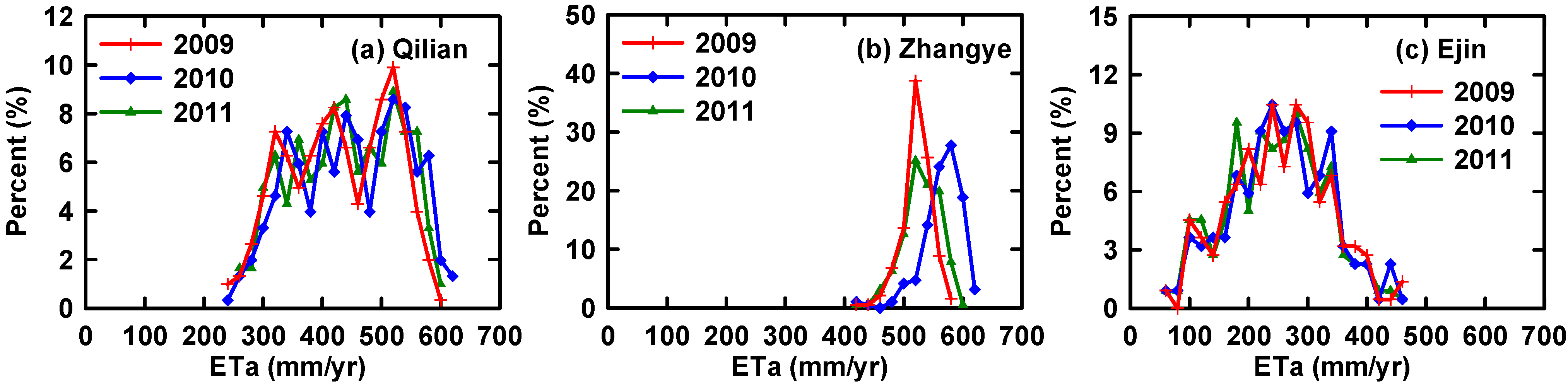
5.3.1. Characteristics of ETa in the Upstream, Middle Stream and Downstream Areas


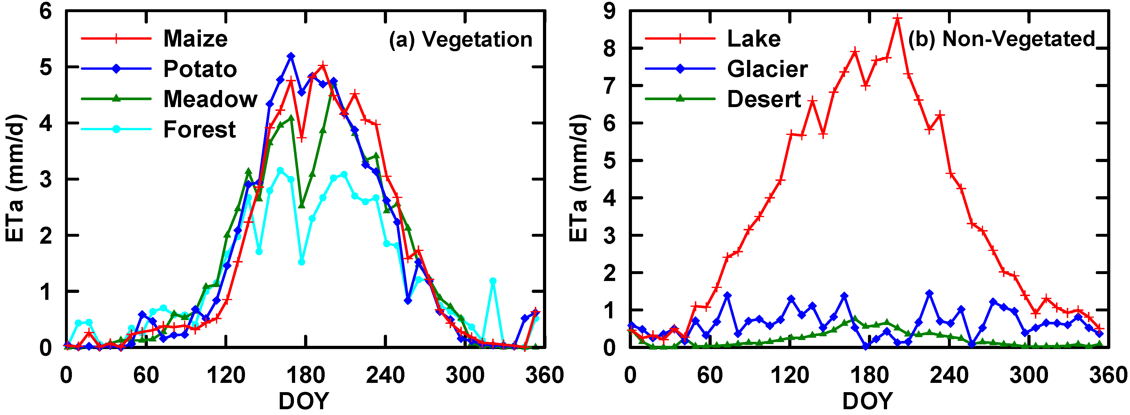
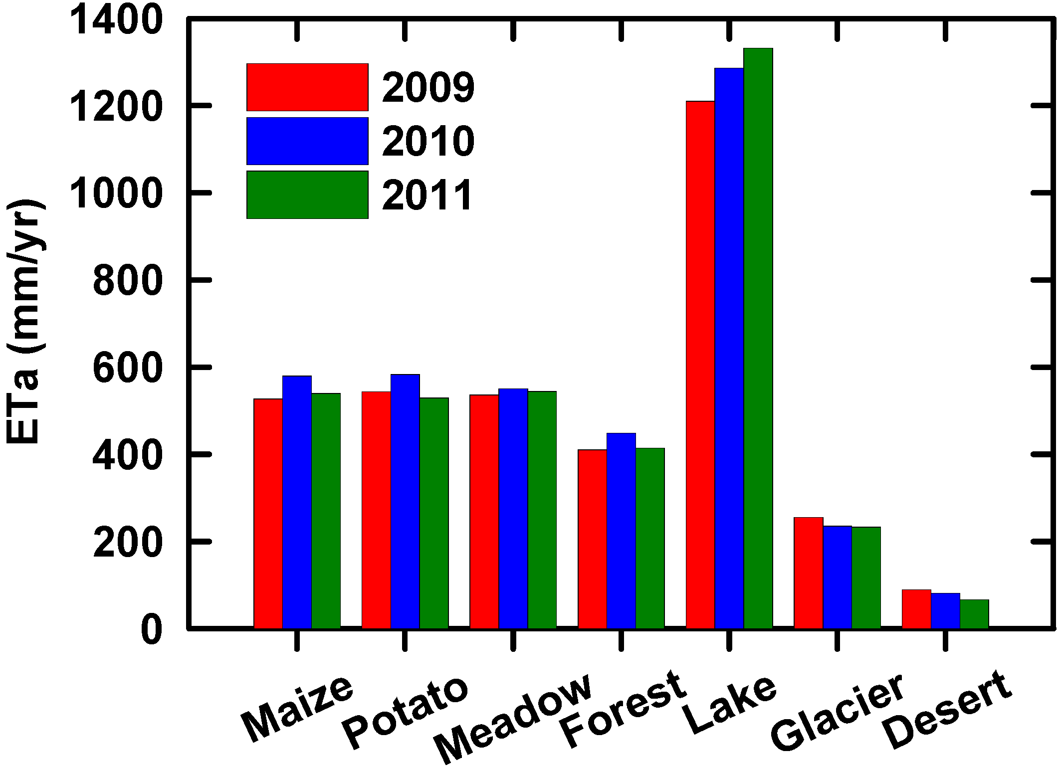
5.3.2. Land Cover Dependence and Temporal Variation


6. Discussion
7. Conclusions
Acknowledgments
Author Contributions
Conflicts of Interest
References
- Nian, Y.Y.; Li, X.; Zhou, J.; Hu, X.L. Impact of land use change on water resource allocation in the middle reaches of the Heihe River Basin in northwestern China. J. Arid Land 2014, 6, 273–286. [Google Scholar] [CrossRef]
- Zeng, Z.; Liu, J.; Koeneman, P.H.; Zarate, E.; Hoekstra, A.Y. Assessing water footprint at river basin level: A case study for the Heihe River Basin in northwest China. Hydrol. Earth Syst. Sci. 2012, 16, 2771–2781. [Google Scholar] [CrossRef]
- Ge, Y.C.; Li, X.; Huang, C.L.; Nan, Z.T. A Decision Support System for irrigation water allocation along the middle reaches of the Heihe River Basin, Northwest China. Environ. Model. Softw. 2013, 47, 182–192. [Google Scholar] [CrossRef]
- Leuning, R.; Zhang, Y.Q.; Rajaud, A.; Cleugh, H.; Tu, K. A simple surface conductance model to estimate regional evaporation using MODIS leaf area index and the Penman–Monteith equation. Water Resour. Res. 2008. [Google Scholar] [CrossRef]
- Carlson, T.N.; Capehart, W.J.; Gillies, R.R. A new look at the simplified method for remote sensing of daily evapotranspiration. Remote Sens. Environ. 1995, 54, 161–167. [Google Scholar] [CrossRef]
- Wang, K.C.; Liang, S.L. An improved method for estimating global evapotranspiration based on satellite determination of surface net radiation, vegetation index, temperature, and soil moisture. J. Hydrometeorol. 2008, 9, 712–727. [Google Scholar] [CrossRef]
- Garcia, M.; Fernández, N.; Villagarcía, L.; Domingo, F.; Puigdefábregas, J.; Sandholt, I. Accuracy of the Temperature-Vegetation Dryness Index using MODIS under water-limited vs. energy-limited evapotranspiration conditions. Remote Sens. Environ. 2014, 149, 100–117. [Google Scholar] [CrossRef]
- Jiang, L.; Islam, S. A methodology for estimation of surface evapotranspiration over large areas using remote sensing observations. Geophys. Res. Lett. 1999, 26, 2773–2776. [Google Scholar] [CrossRef]
- Tang, R.L.; Li, Z.L.; Tang, B.H. An application of the Ts–VI triangle method with enhanced edges determination for evapotranspiration estimation from MODIS data in arid and semi-arid regions: Implementation and validation. Remote Sens. Environ. 2010, 114, 540–551. [Google Scholar] [CrossRef]
- Bastiaanssen, W.G.M.; Menenti, M.; Feddes, R.A.; Holtslag, A.A.M. A remote sensing surface energy balance algorithm for land (SEBAL): 1. Formulation. J. Hydrol. 1998, 212, 198–212. [Google Scholar] [CrossRef]
- Jia, L.; Su, Z.; van den Hurk, B.; Menenti, M.; Moene, A.; De Bruin, H.A.R.; Yrisarry, J.J.B.; Ibanez, M.; Cuesta, A. Estimation of sensible heat flux using the Surface Energy Balance System (SEBS) and ATSR measurements. Phys. Chem. Earth 2003, 28, 75–88. [Google Scholar] [CrossRef]
- Kustas, W.P.; Norman, J.M. Evaluation of soil and vegetation heat flux predictions using a simple two-source model with radiometric temperatures for partial canopy cover. Agric. For. Meteorol. 1999, 94, 13–29. [Google Scholar] [CrossRef]
- Norman, J.M.; Kustas, W.P.; Humes, K.S. Source approach for estimating soil and vegetation energy fluxes in observations of directional radiometric surface temperature. Agric. For. Meteorol. 1995, 77, 263–293. [Google Scholar] [CrossRef]
- Su, Z. The Surface Energy Balance System (SEBS) for estimation of turbulent heat fluxes. Hydrol. Earth Syst. Sci. 2002, 6, 85–99. [Google Scholar] [CrossRef]
- Bastiaanssen, W.G.M.; Cheema, M.J.M.; Immerzeel, W.W.; Miltenburg, I.J.; Pelgrum, H. Surface energy balance and actual evapotranspiration of the transboundary Indus Basin estimated from satellite measurements and the ETLook model. Water Resour. Res. 2012. [Google Scholar] [CrossRef]
- Cleugh, H.A.; Leuning, R.; Mu, Q.; Running, S.W. Regional evaporation estimates from flux tower and MODIS satellite data. Remote Sens. Environ. 2007, 106, 285–304. [Google Scholar] [CrossRef]
- Fisher, J.B.; Tu, K.P.; Baldocchi, D.D. Global estimates of the land atmosphere water flux based on monthly AVHRR and ISLSCP-II data, validated at FLUXNET sites. Remote Sens. Environ. 2008, 112, 901–919. [Google Scholar] [CrossRef]
- Mu, Q.Z.; Heinsch, F.A.; Zhao, M.S.; Running, S.W. Development of a global evapotranspiration algorithm based on MODIS and global meteorology data. Remote Sens. Environ. 2007, 111, 519–536. [Google Scholar] [CrossRef]
- Mu, Q.Z.; Zhao, M.S.; Running, S.W. Improvements to a MODIS global terrestrial evapotranspiration algorithm. Remote Sens. Environ. 2011, 115, 1781–1800. [Google Scholar] [CrossRef]
- Courault, D.; Seguin, B.; Olioso, A. Review on estimation of evapotranspiration from remote sensing data: From empirical to numerical modeling approaches. Irrig. Drain. Syst. 2005, 19, 223–249. [Google Scholar] [CrossRef]
- Kalma, J.D.; McVicar, T.R.; McCabe, M.F. Estimating land surface evaporation: A review of methods using remotely sensed surface temperature data. Surv. Geophys. 2008, 29, 421–469. [Google Scholar] [CrossRef]
- Li, Z.L.; Tang, R.L.; Wan, Z.; Bi, Y.; Zhou, C.; Tang, B.H.; Yan, G.J.; Zhang, X. A review of current methodologies for regional evapotranspiration estimation from remotely sensed data. Sensors 2009, 9, 3801–3853. [Google Scholar] [CrossRef] [PubMed]
- Li, S.B.; Zhao, W.Z. Satellite-based actual evapotranspiration estimation in the middle reach of the Heihe River Basin using the SEBAL method. Hydrol. Process. 2010, 24, 3337–3344. [Google Scholar] [CrossRef]
- Yang, Y.M.; Su, H.B.; Zhang, R.H.; Tian, J.; Yang, S.Q. Estimation of regional evapotranspiration based on remote sensing: Case study in the Heihe River Basin. J. Appl. Remote Sens. 2012. [Google Scholar] [CrossRef]
- Li, Z.L.; Tang, B.H.; Wu, H.; Ren, H.Z.; Yan, G.J.; Wan, Z.M.; Trigo, I.F.; Sobrino, J.A. Satellite-derived land surface temperature: Current status and perspectives. Remote Sens. Environ. 2013, 131, 14–37. [Google Scholar] [CrossRef]
- Ghilain, N.; Arboleda, A.; Sepulcre-Canto, G.; Batelaan, O.; Ardo, J.; Gellens-Meulenberghs, F. Improving evapotranspiration in a land surface model using biophysical variables derived from MSG/SEVIRI satellite. Hydrol. Earth Syst. Sci. 2012, 16, 2567–2583. [Google Scholar] [CrossRef]
- Monteith, J.L. Evaporation and environment. In The State and Movement of Water in Living Organisms. Symposium of the Society of Experimental Biology; Fogg, G.E., Ed.; Society of Experimental Biology, Cambridge University Press: Swansea, UK, 1965; Volume 19, pp. 205–234. [Google Scholar]
- Liang, X.; Lettenmaier, D.P.; Wood, E.F.; Burges, S.J. A simple hydrologically based model of land surface water and energy fluxes for general circulation models. J. Geophys. Res. 1994, 99, 14415–14428. [Google Scholar] [CrossRef]
- Sellers, P.J.; Randall, D.A.; Collatz, G.J.; Berry, J.A.; Field, C.B.; Dazlich, D.A.; Zhang, C.; Collelo, G.D.; Bounoua, L. A revised land surface parameterization (SiB2) for atmospheric GCMs. Part I: Model formulation. J. Clim. 1996, 9, 676–705. [Google Scholar] [CrossRef]
- Shuttleworth, W.J.; Wallace, J.S. Evaporation from sparse crops—An energy combination theory. Q. J. R. Meteorol. Soc. 1985, 111, 839–855. [Google Scholar] [CrossRef]
- Anadranistakis, M.; Liakatas, A.; Kerkides, P.; Rizosb, S.; Gavanosisb, J.; Poulovassilis, A. Crop water requirements model tested for crops grown in Greece. Agric. Water Manag. 2000, 45, 297–316. [Google Scholar] [CrossRef]
- Shaw, R.H.; Pereira, A.R. Aerodynamic roughness of a plant canopy: A numerical experiment. Agric. Meteorol. 1982, 26, 51–65. [Google Scholar] [CrossRef]
- Gutman, G.; Ignatov, V. The derivation of the green vegetation fraction from NOAA/AVHRR data for use in numerical weather prediction models. Int. J. Remote Sens. 1998, 19, 1533–1543. [Google Scholar] [CrossRef]
- Camillo, P.J.; Gurney, R.J. A resistance parameter for bare-soil evaporation models. Soil Sci. 1986, 141, 95–105. [Google Scholar] [CrossRef]
- Clapp, R.B.; Hornberger, G.M. Empirical equations for some soil hydraulic properties. Water Resour. Res. 1978, 14, 601–604. [Google Scholar] [CrossRef]
- Dolman, A.J. A multiple-source land surface energy balance model for use in general circulation models. Agric. For. Meteorol. 1993, 65, 21–45. [Google Scholar] [CrossRef]
- Van Genuchten, M.T. A closed-form equation for predicting the hydraulic conductivity of unsaturated soils. Soil Sci. Soc. Am. J. 1980, 44, 892–898. [Google Scholar] [CrossRef]
- Avissar, R.; Avissar, P.; Mahrer, Y.; Bravdo, B.A. A model to simulate response of plant stomata to environmental conditions. Agric. For. Meteorol. 1985, 34, 21–29. [Google Scholar] [CrossRef]
- Jarvis, P.G. The interpretation of the variations in leaf water potential and stomatal conductance found in canopies in the field. Philos. Trans. R. Soc. Lond. B 1976, 273, 593–610. [Google Scholar] [CrossRef]
- Stewart, J.B. Modelling surface conductance of pine forest. Agric. For. Meteorol. 1988, 43, 19–35. [Google Scholar] [CrossRef]
- Mehrez, M.B.; Taconet, O.; Vidal-Madjar, D.; Valencogne, C. Estimation of stomatal resistance and canopy evaporation during the HAPEX–MOBILHY experiment. Agric. For. Meteorol. 1992, 58, 285–313. [Google Scholar] [CrossRef]
- Dickinson, R.E. Modelling evapotranspiration for three-dimensional global climate models. Geophys. Monogr. Ser. 1984, 29, 58–72. [Google Scholar]
- Irannejad, P.; Shao, Y.P. Description and validation of the atmosphere–land–surface interaction scheme (ALSIS) with HAPEX and Cabauw data. Glob. Planet. Chang. 1998, 19, 87–114. [Google Scholar] [CrossRef]
- Mo, X.G.; Liu, S.X.; Lin, Z.H.; Zhao, W.M. Simulating temporal and spatial variation of evapotranspiration over the Lushi basin. J. Hydrol. 2004, 285, 125–142. [Google Scholar] [CrossRef]
- Sellers, P.J.; Mintz, Y.; Sud, Y.C.; Dalcher, A. A simple biosphere model (SiB) for use within general circulation models. J. Atmos. Sci. 1986, 43, 505–531. [Google Scholar] [CrossRef]
- Noilhan, J.; Planton, S. A simple parameterization of land surface processes for meteorological models. Mon. Weather Rev. 1989, 117, 536–549. [Google Scholar] [CrossRef]
- Allen, R.G.; Pruitt, W.O.; Businger, J.A.; Fritschen, L.J.; Jensen, M.E.; Quinn, F.H. Evaporation and transpiration. In Hydrology Handbook, 2nd ed.; Task Committee on Hydrology Handbook of Management Group D of American Society of Civil Engineers (ASCE), Ed.; ASCE: New York, NY, USA, 1996; pp. 125–252. [Google Scholar]
- Gash, J.H.C.; Lloyd, C.R.; Lachaud, G. Estimating sparse forest rainfall interception with an analytical model. J. Hydrol. 1995, 170, 79–86. [Google Scholar] [CrossRef]
- Van Dijk, A.I.J.M.; Bruijnzeel, L.A. Modelling rainfall interception by vegetation of variable density using an adapted analytical model. Part 1. Model description. J. Hydrol. 2001, 247, 230–238. [Google Scholar] [CrossRef]
- Cui, Y.K.; Jia, L. A modified Gash model for estimating rainfall interception loss of forest using remote sensing observations at regional scale. Water 2014, 6, 993–1012. [Google Scholar] [CrossRef]
- Cui, Y.K.; Jia, L.; Hu, G.C.; Zhou, J. Mapping of interception loss of vegetation in the Heihe River basin of China using remote sensing observations. IEEE Geosci. Remote Sens. Lett. 2015, 12, 23–27. [Google Scholar] [CrossRef]
- Kuzmin, P.P. On method for investigations of evaporation from the snow cover. Trans. State Hydrol. Inst. 1953, 41, 34–52. (In Russian) [Google Scholar]
- Penman, H.L. Natural evaporation from open water, bare soil and grass. Proc. R. Soc. A 1948, 193, 120–145. [Google Scholar] [CrossRef]
- Liu, Q.; Wang, L.; Qu, Y.; Liu, N.; Liu, S.; Tang, H.; Liang, S. Preliminary evaluation of the long-term GLASS albedo product. Int. J. Digit. Earth 2013, 6, 69–95. [Google Scholar] [CrossRef]
- Jia, L.; Shang, H.; Hu, G.; Menenti, M. Phenological response of vegetation to upstream river flow in the Heihe River basin by time series analysis of MODIS data. Hydrol. Earth Syst. Sci. 2011, 15, 1047–1064. [Google Scholar] [CrossRef]
- Ran, Y.H.; Li, X.; Lu, L.; Li, Z.Y. Large-scale land cover mapping with the integration of multi-source information based on the Dempster–Shafer theory. Int. J. Geogr. Inf. Sci. 2012, 26, 169–191. [Google Scholar] [CrossRef]
- Zhong, B.; Ma, P.; Nie, A.H.; Yang, A.X.; Yao, Y.J.; Lv, W.B.; Zhang, H.; Liu, Q.H. Land cover mapping using time series HJ-1/CCD data. Sci. China Earth Sci. 2014, 57, 1790–1799. [Google Scholar] [CrossRef]
- Dai, Y.J.; Shangguan, W.; Duan, Q.Y.; Liu, B.; Fu, S.; Niu, G. Development of a China dataset of soil hydraulic parameters using pedotransfer functions for land surface modeling. J. Hydrometeorol. 2013, 14, 869–887. [Google Scholar] [CrossRef]
- Pan, X.D.; Li, X. Validation of WRF model on simulating forcing data for Heihe River Basin. Sci. Cold Arid Region. 2011, 3, 344–357. [Google Scholar]
- Pan, X.D.; Li, X.; Shi, X.K.; Han, X.J.; Luo, L.H.; Wang, L.X. Dynamic downscaling of near-surface air temperature at the basin scale using WRF—A case study in the Heihe River Basin, China. Front. Earth Sci. 2012, 6, 314–323. [Google Scholar] [CrossRef]
- Gao, Y.C.; Long, D.; Li, Z.L. Estimation of daily actual evapotranspiration from remotely sensed data under complex terrain over the upper Chao river basin in North China. Int. J. Remote Sens. 2008, 29, 3295–3315. [Google Scholar] [CrossRef]
- Stahl, K.; Moore, R.D.; Floyer, J.A.; Asplin, M.G.; McKendry, I.G. Comparison of approaches for spatial interpolation of daily air temperature in a large region with complex topography and highly variable station density. Agric. For. Meteorol. 2006, 139, 224–236. [Google Scholar] [CrossRef]
- Li, X.; Li, X.W.; Li, Z.Y.; Ma, M.G.; Wang, J.; Xiao, Q.; Liu, Q.; Che, T.; Chen, E.X.; Yan, G.J.; et al. Watershed allied telemetry experimental research. J. Geophys. Res. 2009. [Google Scholar] [CrossRef]
- Li, X.; Cheng, G.D.; Liu, S.M.; Xiao, Q.; Ma, M.G.; Jin, R.; Che, T.; Liu, Q.H.; Wang, W.Z.; Qi, Y.; et al. Heihe Watershed Allied Telemetry Experimental Research (HiWATER) scientific objectives and experimental design. Bull. Am. Meteorol. Soc. 2013, 94, 1145–1160. [Google Scholar] [CrossRef]
- Liu, S.M.; Xu, Z.W.; Wang, W.Z.; Jia, Z.Z.; Zhu, M.J.; Bai, J.; Wang, J.M. A comparison of eddy-covariance and large aperture scintillometer measurements with respect to the energy balance closure problem. Hydrol. Earth Syst. Sci. 2011, 15, 1291–1306. [Google Scholar] [CrossRef]
- Blanken, P.D.; Black, T.A.; Neumann, H.H.; Den Hartog, G.; Yang, P.C.; Nesic, Z.; Staebler, R.; Chen, W.; Novak, M.D. Turbulent flux measurements above and below the overstory of a boreal aspen forest. Bound. Layer Meteorol. 1998, 89, 109–140. [Google Scholar] [CrossRef]
- Goulden, M.L.; Daube, B.C.; Fan, S.M.; Sutton, D.J.; Bazzaz, A.; Munger, J.W.; Wofsy, S.C. Physiological responses of a black spruce forest to weather. J. Geophys. Res. 1997, 102, 28987–28996. [Google Scholar] [CrossRef]
- Meyers, T.P.; Hollinger, S.E. An assessment of storage terms in the surface energy balance of maize and soybean. Agric. For. Meteorol. 2004, 125, 105–115. [Google Scholar] [CrossRef]
- Twine, T.E.; Kustas, W.P.; Norman, J.M.; Cook, D.R.; Houser, P.R.; Meyers, T.P.; Prueger, J.H.; Starks, P.J.; Wesely, M.L. Correcting eddy-covariance flux underestimates over a grassland. Agric. For. Meteorol. 2000, 103, 279–300. [Google Scholar] [CrossRef]
- Kustas, W.P.; Norman, J.M. Evaluating the effects of subpixel heterogeneity on pixel average fluxes. Remote Sens. Environ. 2000, 74, 327–342. [Google Scholar] [CrossRef]
- Kustas, W.P.; Li, F.; Jackson, T.J.; Prueger, J.H.; MacPherson, J.I.; Wolde, M. Effects of remote sensing pixel resolution on modeled energy flux variability of croplands in Iowa. Remote Sens. Environ. 2004, 92, 535–547. [Google Scholar] [CrossRef]
- Li, F.; Kustas, W.P.; Anderson, M.C.; Prueger, J.H.; Scott, R.L. Effect of remote sensing spatial resolution on interpreting tower-based flux observations. Remote Sens. Environ. 2008, 112, 337–349. [Google Scholar] [CrossRef]
- Chen, Y.Y.; Yang, K.; Qin, J.; Zhao, L.; Tang, W.J.; Han, M.L. Evaluation of AMSR-E retrievals and GLDAS simulations against observations of a soil moisture network on the central Tibetan Plateau. J. Geophys. Res. Atmos. 2013, 118, 4466–4475. [Google Scholar] [CrossRef]
- Yang, K.; Qin, J.; Zhao, L.; Chen, Y.Y.; Tang, W.J.; Han, M.L.; Lazhu; Chen, Z.Q.; Lv, N.; Ding, B.H.; et al. A multi-scale soil moisture and freeze-thaw monitoring network on the Third Pole. Bull. Am. Meteorol. Soc. 2013, 94, 1907–1916. [Google Scholar] [CrossRef]
- Xue, B.L.; Wang, L.; Li, X.P.; Yang, K.; Chen, D.L.; Sun, L.T. Evaluation of evapotranspiration estimates for two river basins on the Tibetan Plateau by a water balance method. J. Hydrol. 2013, 492, 290–297. [Google Scholar] [CrossRef]
- Zhan, X.; Kustas, W.P.; Humes, K.S. An intercomparison study on models of sensible heat flux over partial canopy surfaces with remotely sensed surface temperature. Remote Sens. Environ. 1996, 58, 242–256. [Google Scholar] [CrossRef]
- Cheng, G.D. Integrated Management of the Water–Ecology–Economy System in the Heihe River Basin; Science Press: Beijing, China, 2009. (In Chinese) [Google Scholar]
- Decker, M.; Brunke, M.A.; Wang, Z.; Sakaguchi, K.; Zeng, X.B.; Bosilovich, M.G. Evaluation of the reanalysis products from GSFC, NCEP, and ECMWF using flux tower observations. J. Clim. 2012, 25, 1916–1944. [Google Scholar] [CrossRef]
- Liston, G.E.; Elder, K. A meteorological distribution system for high-resolution terrestrial modeling (MicroMet). J. Hydrometeorol. 2006, 7, 217–234. [Google Scholar] [CrossRef]
- McVicar, T.R.; Van Niel, T.G.; Li, L.T.; Hutchinson, M.F.; Mu, X.M.; Liu, Z.H. Spatially distributing monthly reference evapotranspiration and pan evaporation considering topographic influences. J. Hydrol. 2007, 338, 196–220. [Google Scholar] [CrossRef]
- Liu, Q.; Du, J.Y.; Shi, J.C.; Jiang, L.M. Analysis of spatial distribution and multi-year trend of the remotely sensed soil moisture on the Tibetan Plateau. Sci. China Earth Sci. 2013, 56, 2173–2185. [Google Scholar] [CrossRef]
- Shi, J.C.; Du, Y.; Du, J.Y.; Jiang, L.M.; Chai, L.N.; Mao, K.B.; Xu, P.; Ni, W.J.; Xiong, C.; Liu, Q.; et al. Progresses on microwave remote sensing of land surface parameters. Sci. China Earth Sci. 2012, 55, 1052–1078. [Google Scholar] [CrossRef]
- Das, N.N.; Entekhabi, D.; Njoku, E.G. An algorithm for merging SMAP radiometer and radar data for high-resolution soil-moisture retrieval. IEEE Trans. Geosci. Remote Sens. 2011, 49, 1504–1512. [Google Scholar] [CrossRef]
- Song, C.Y.; Jia, L.; Menenti, M. Retrieving high-resolution surface soil moisture by downscaling AMSR-E brightness temperature using MODIS LST and NDVI data. IEEE J. Sel. Top. Appl. Earth Obs. Remote Sens. 2014, 7, 935–942. [Google Scholar] [CrossRef]
- Liu, S.M.; Xu, Z.W.; Zhu, Z.L.; Jia, Z.Z.; Zhu, M.J. Measurements of evapotranspiration from eddy-covariance systems and large aperture scintillometers in the Hai River Basin, China. J. Hydrol. 2013, 487, 24–38. [Google Scholar] [CrossRef]
- Liu, Z.J.; Shao, Q.Q.; Liu, J.Y. The performances of MODIS-GPP and -ET products in China and their sensitivity to input data (FPAR/LAI). Remote Sens. 2015, 7, 135–152. [Google Scholar] [CrossRef]
- Velpuri, N.M.; Senay, G.B.; Singh, R.K.; Bohms, S.; Verdin, J.P. A comprehensive evaluation of two MODIS evapotranspiration products over the conterminous United States: Using point and gridded FLUXNET and water balance ET. Remote Sens. Environ. 2013, 139, 35–49. [Google Scholar] [CrossRef]
- Ruhoff, A.L.; Paz, A.R.; Aragao, L.E.O.C.; Mu, Q.; Malhi, Y.; Collischonn, W.; Rocha, H.R.; Running, S.W. Assessment of the MODIS global evapotranspiration algorithm using eddy covariance measurements and hydrological modelling in the Rio Grande basin. Hydrol. Sci. J. 2013, 58, 1–19. [Google Scholar] [CrossRef]
- Ramoelo, A.; Majozi, N.; Mathieu, R.; Jovanovic, N.; Nickless, A.; Dzikiti, S. Validation of global evapotranspiration product (MOD16) using flux tower data in the African savanna, South Africa. Remote Sens. 2014, 6, 7406–7423. [Google Scholar] [CrossRef]
- Hu, G.C.; Jia, L.; Menenti, M. Comparison of MOD16 and LSA-SAF MSG evapotranspiration products over Europe for 2011. Remote Sens. Environ. 2015, 156, 510–526. [Google Scholar] [CrossRef]
- Garcia, M.; Sandholt, I.; Ceccato, P.; Ridler, M.; Mougin, E.; Kergoat, L.; Morillas, L.; Timouk, F.; Fensholt, R.; Domingo, F. Actual evapotranspiration in drylands derived from in-situ and satellite data: Assessing biophysical constraints. Remote Sens. Environ. 2013, 131, 103–118. [Google Scholar] [CrossRef]
- Vinukollu, R.K.; Wood, E.F.; Ferguson, C.R.; Fisher, J.B. Global estimates of evapotranspiration for climate studies using multi-sensor remote sensing data: Evaluation of three process-based approaches. Remote Sens. Environ. 2011, 115, 801–823. [Google Scholar] [CrossRef]
- Cheng, G.D.; Li, X.; Zhao, W.Z.; Xu, Z.M.; Feng, Q.; Xiao, S.C.; Xiao, H.L. Integrated study of the water–ecosystem–economy in the Heihe River Basin. Natl. Sci. Rev. 2014, 1, 413–428. [Google Scholar] [CrossRef]
© 2015 by the authors; licensee MDPI, Basel, Switzerland. This article is an open access article distributed under the terms and conditions of the Creative Commons Attribution license (http://creativecommons.org/licenses/by/4.0/).
Share and Cite
Hu, G.; Jia, L. Monitoring of Evapotranspiration in a Semi-Arid Inland River Basin by Combining Microwave and Optical Remote Sensing Observations. Remote Sens. 2015, 7, 3056-3087. https://doi.org/10.3390/rs70303056
Hu G, Jia L. Monitoring of Evapotranspiration in a Semi-Arid Inland River Basin by Combining Microwave and Optical Remote Sensing Observations. Remote Sensing. 2015; 7(3):3056-3087. https://doi.org/10.3390/rs70303056
Chicago/Turabian StyleHu, Guangcheng, and Li Jia. 2015. "Monitoring of Evapotranspiration in a Semi-Arid Inland River Basin by Combining Microwave and Optical Remote Sensing Observations" Remote Sensing 7, no. 3: 3056-3087. https://doi.org/10.3390/rs70303056