
Estimation of Actual Crop Coefficients Using Remotely Sensed Vegetation Indices and Soil Water Balance Modelled Data


Abstract
:
1. Introduction
2. Material and Methods
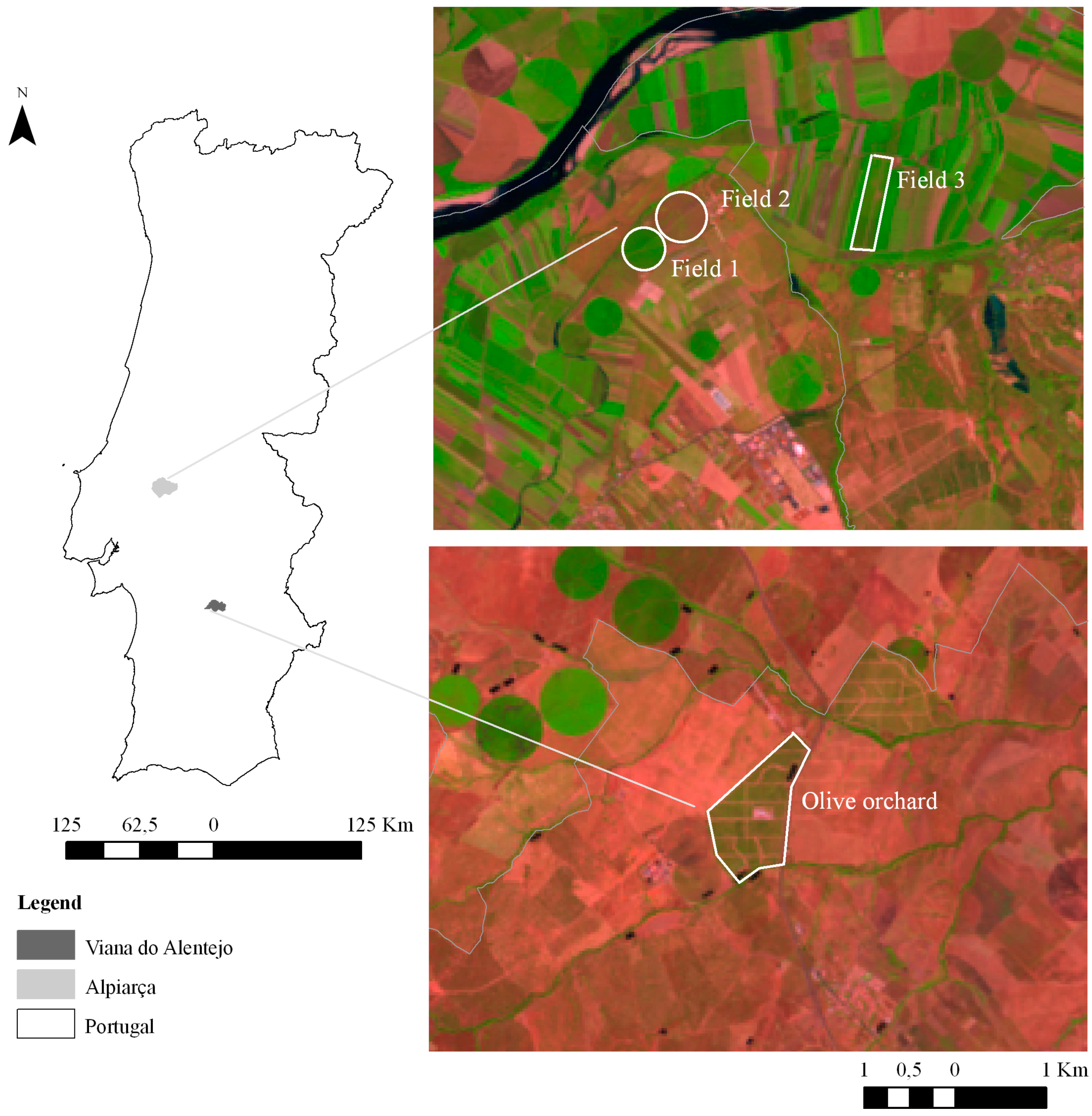
2.1. Study Areas


| Crop Growth Stages | Maize Study Areas | Barley Study Areas |
|---|---|---|
| Field 1—Year 2010 | 2012 season | |
| Initial (Ini) | 25/05–25/06 | 16/01–06/02 |
| Development (Dev) | 26/06–22/07 | 07/02–03/04 |
| Mid-season (Mid) | 23/07–04/09 | 04/04–20/05 |
| Late-season (Late) | 05/09–13/10 | 21/05–26/06 |
| Field 2—Year 2010 | 2012/2013 season | |
| Initial (Ini) | 25/05–25/06 | 06/12–12/01 |
| Development (Dev) | 26/06–17/07 | 13/01–10/03 |
| Mid-season (Mid) | 18/07–02/09 | 11/03–05/05 |
| Late-season (Late) | 03/09–13/10 | 06/05–06/06 |
| Field 1—Year 2011 | ||
| Initial (Ini) | 20/04–17/05 | |
| Development (Dev) | 18/05–28/06 | |
| Mid-season (Mid) | 29/06–17/08 | |
| Late-season (Late) | 18/08–20/09 | |
| Field 2—Year 2012 | ||
| Initial (Ini) | 16/04–08/05 | |
| Development (Dev) | 09/05 24/06 | |
| Mid-season (Mid) | 25/06–20/08 | |
| Late-season (Late) | 21/08–20/09 | |
| Field 3—Year 2012 | ||
| Initial (Ini) | 30/05–12/06 | |
| Development (Dev) | 13/06–15/07 | |
| Mid-season (Mid) | 16/07–13/09 | |
| Late-season (Late) | 14/09–12/10 |
2.2. Satellite Imagery
| Olive Study Area (203/033) | Maize Study Areas (204/033) | Barley Study Areas (204/033) | |||
|---|---|---|---|---|---|
| Field 1 | Field 2 | Field 3 | 2012 | 2012–2013 | |
| 31/01/2011 (1) | 06/07/2010 (2) | 06/07/2010 (2),* | 11/07/2012 (2) | 02/02/2012 (1) | 03/01/2013(1) |
| 20/03/2011 (2) | 22/07/2010 (3),* | 22/07/2010 (3) | 13/09/2012 (3) | 18/02/2012 (2) | 25/04/2013(3) |
| 05/04/2011 (2) | 30/07/2010 (3),* | 30/07/2010 (3),* | 29/09/2012 (4) | 05/03/2012 (2) | 11/05/2013(4) |
| 23/05/2011 (3) | 15/06/2011 (2) | 11/07/2012 (3) | 21/03/2012 (2) | ||
| 24/06/2011 (3) | 25/07/2011 (3) | 13/09/2012 (4) | 24/05/2012 (4),* | ||
| 26/07/2011 (3) | 18/08/2011 (3) | ||||
| 27/08/2011 (3),* | 19/09/2011 (4) | ||||
| 12/09/2011 (3) | |||||
| 06/10/2011 (4),* | |||||
| 11/02/2012 (1) | |||||
| 15/04/2012 (2),* | |||||
| 20/07/2012 (3),* | |||||
| 21/08/2012 (3),* | |||||
| 06/09/2012 (3) | |||||
| 08/10/2012 (4) | |||||
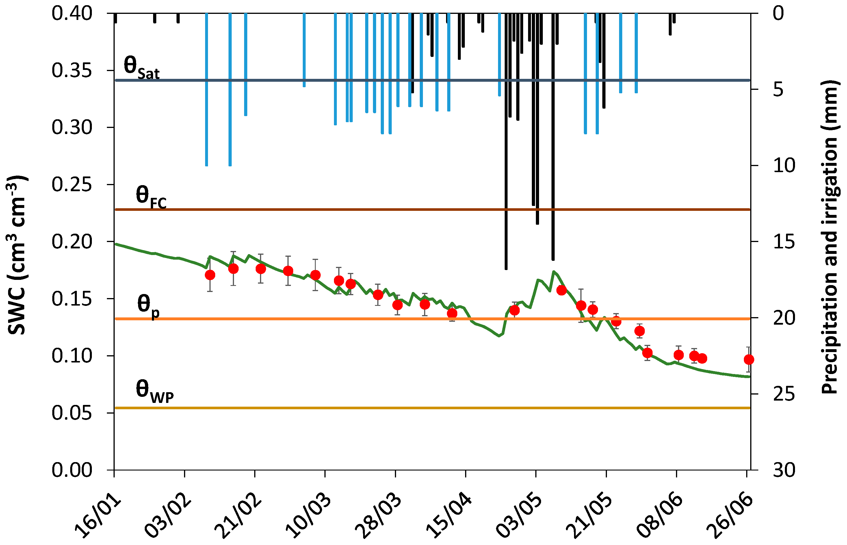
2.3. SIMDualKc

2.4. Basal Crop Coefficients Derived from Reflectance Vegetation Indices
| Kd | Maize Study Areas | Barley Study Areas (3) | Olive Study Areas |
|---|---|---|---|
| Kd (fc field) (1) | [0.93–0.99] | 0.90 | [0.62–0.78] |
| Kd (fc VI) (2) | [0.97–1.00] | 0.90 | [0.66–0.70] |
| Parameters | Crop Growth Stage | Value | ||
|---|---|---|---|---|
| Maize | Barley | Olive | ||
| NDVImax | 0.75–0.85 | 0.75–0.85 | 0.75–0.85 | |
| NDVImin | 0.1 | 0.1 | 0.1 | |
| SAVImax | 0.75 | 0.75 | 0.75 | |
| SAVImin | 0.09 | 0.09 | 0.09 | |
| β2 | 0–0.5 (2) | 0–0.5 (2) | 0–0.5 (2) | |
| β1(1) | Ini | 0.3 | 0.3 | 0.4–0.7 |
| Dev | 0.3–1 | 0.3–1 | 1 | |
| Dev (1st sub-stage) | 0.6 | 0.5 | 1 | |
| Dev (2nd sub-stage) | 0.9 | 0.7 | - | |
| Dev (3rd sub-stage) | - | 0.9 | - | |
| Mid | 1 | 1 | - | |
| End | 1 | 1 | 1 | |
3. Results
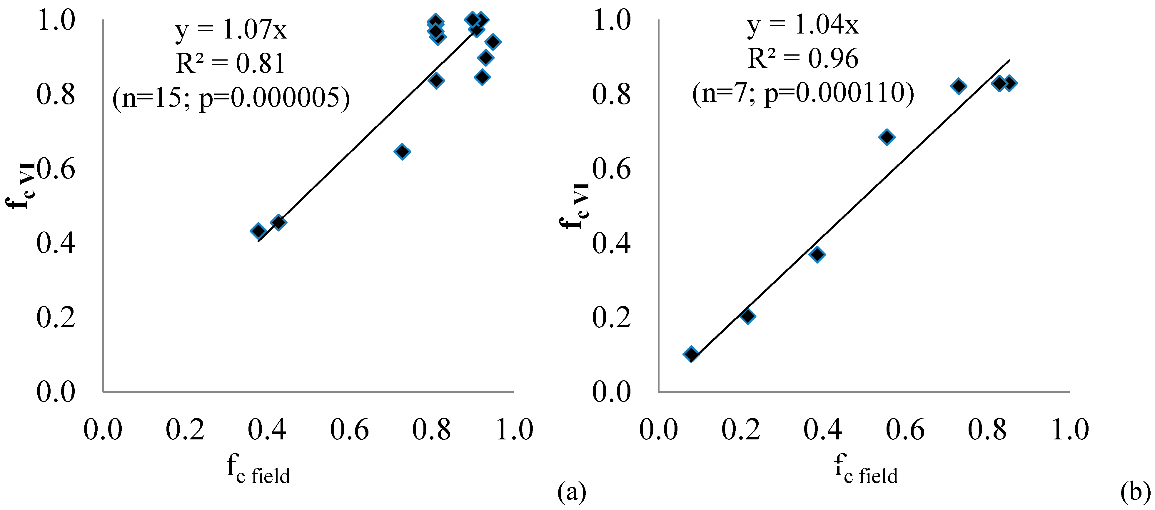
3.1. Estimation of the Fraction of Ground Cover from VI

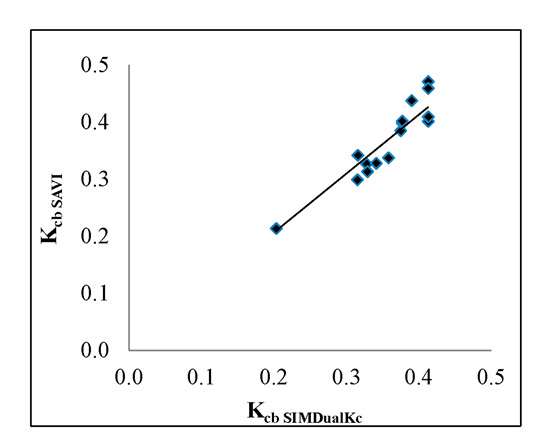
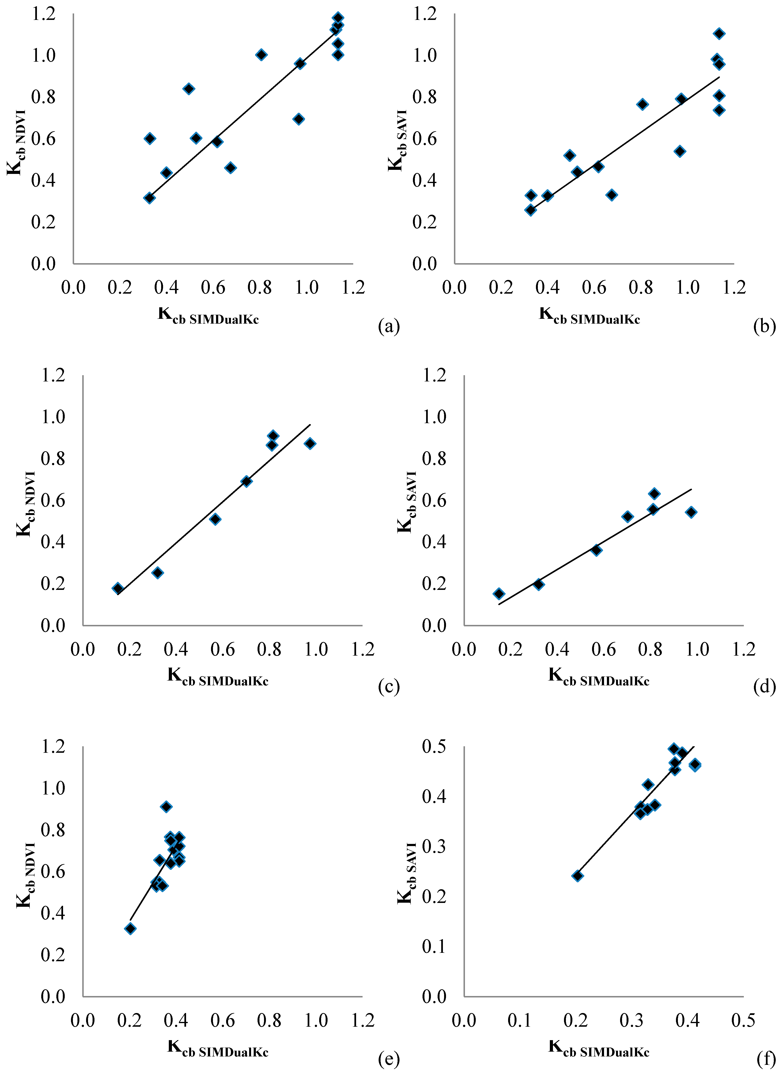
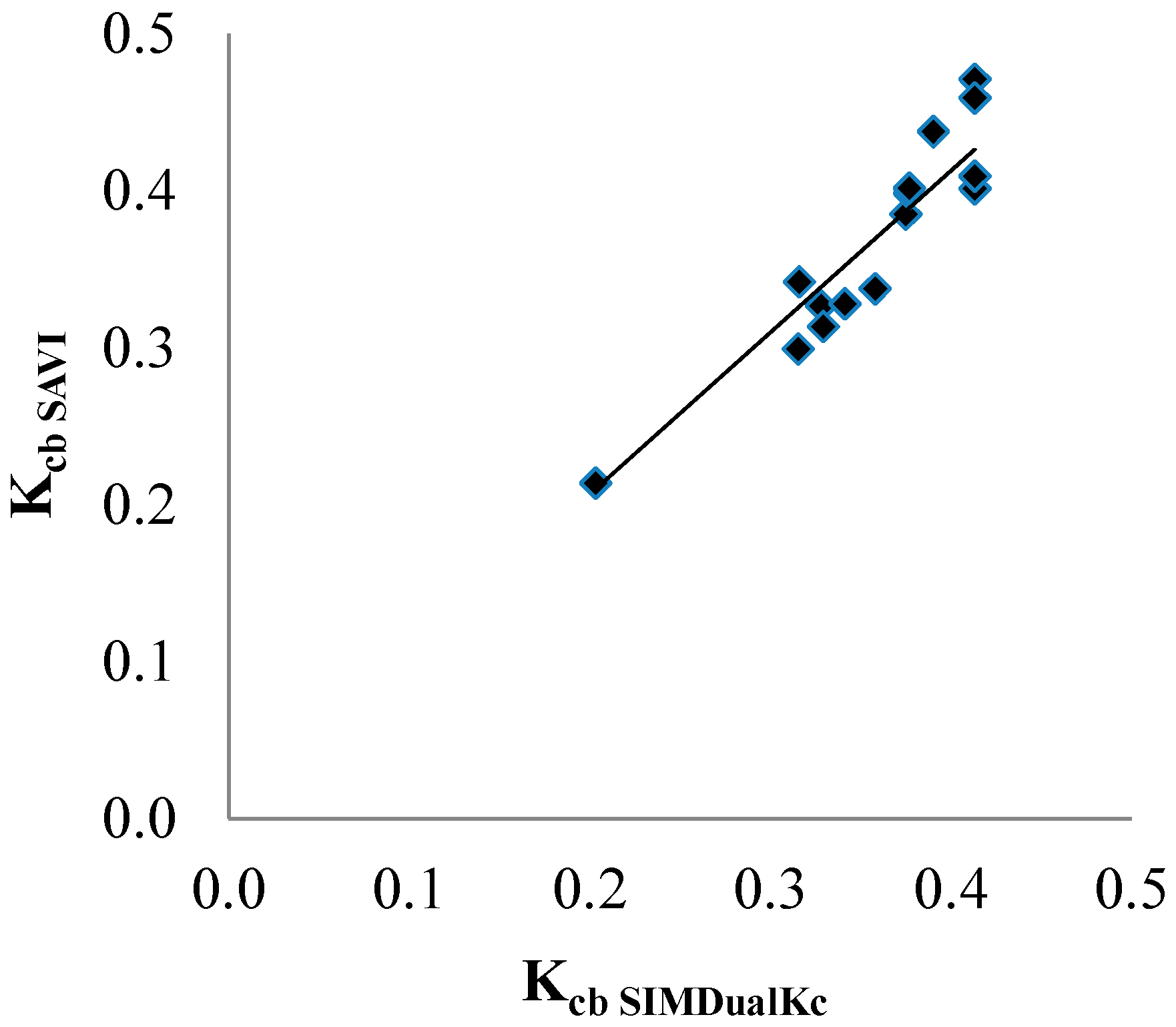
3.2. Estimation of Kcb from Reflectance-Based Vegetation Indices (Kcb VI)

| b | R2 | n | p | Estimation | Cross Validation | ||||
|---|---|---|---|---|---|---|---|---|---|
| RMSD ( ) | RMD (%) | RMSD ( ) | RMD (%) | ||||||
| Maize | Kcb NDVI | 0.98 | 0.74 | 15 | 0.0000389 | 0.16 | 14.8 | 0.08 | 8.4 |
| Kcb SAVI | 0.79 | 0.79 | 15 | 0.0000094 | 0.22 | 21.1 | 0.18 | 20.9 | |
| Barley | Kcb NDVI | 0.99 | 0.95 | 7 | 0.0001935 | 0.07 | 9.6 | 0.04 | 4.7 |
| Kcb SAVI | 0.67 | 0.89 | 7 | 0.0014203 | 0.23 | 32.0 | 0.22 | 31.3 | |
| Olive | Kcb NDVI | 1.81 | 0.56 | 15 | 0.0013317 | 0.31 | 81.1 | 0.30 | 82.5 |
| Kcb SAVI | 1.19 | 0.72 | 15 | 0.0000023 | 0.08 | 21.7 | 0.07 | 19.0 | |
| Kcb SAVI * | 1.03 | 0.88 | 15 | 0.0000002 | 0.02 | 5.6 | 0.01 | 3.3 | |

| Crop Growth Stages | Maize | Barley | Olive |
|---|---|---|---|
| Kcb NDVI | |||
| Initial | (1) | 0.18 ( ) (2) | 0.78 (±0.13) |
| Development (4) | [0.44–1.00] | [0.25–0.91] | [0.53–0.77] (3) |
| Mid-season | 0.92 (±0.11) (5) | 0.87 ( ) (2) | 0.61 (±0.05) (6) |
| Late-season (4) | [0.84–0.46] | [0.86–0.69] | [0.75–0.55] |
| Kcb SAVI | |||
| Initial | (1) | 0.15 ( ) (2) | 0.33 (±0.01) |
| Development (4) | [0.33–0.76] | [0.20–0.63] | [0.30–0.44] (3) |
| Mid-season | 0.76 (±0.10) (5) | 0.54 ( ) (2) | 0.37 (±0.03) (6) |
| Late-season (4) | [0.52–0.33] | [0. 56–0.52] | [0.40–0.33] |


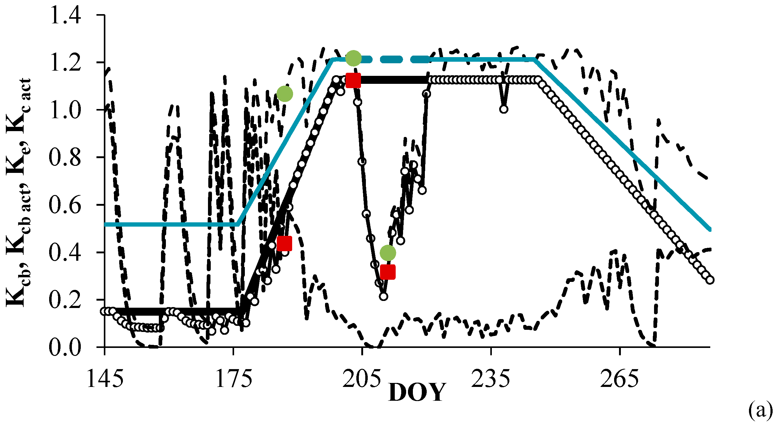
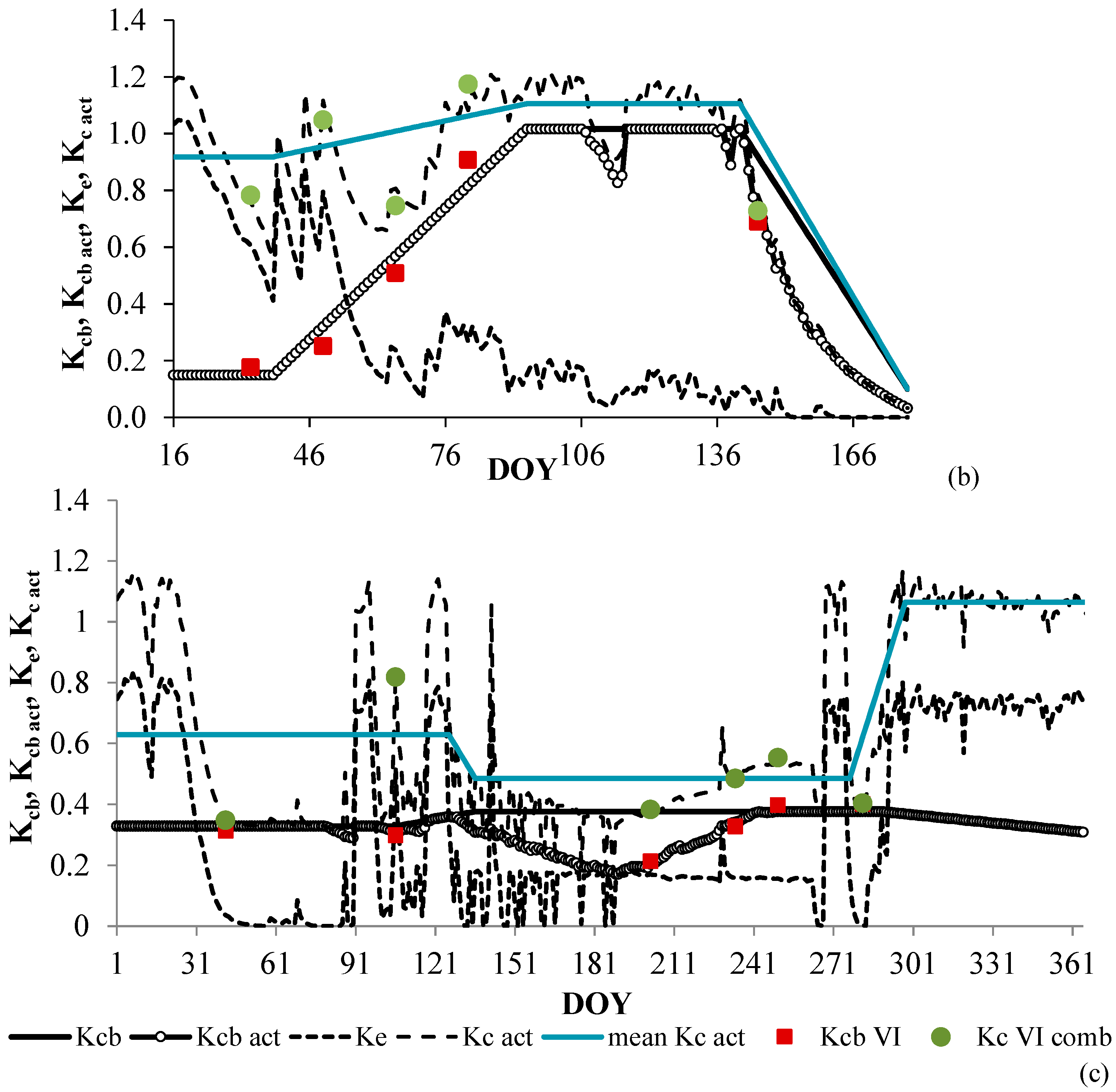
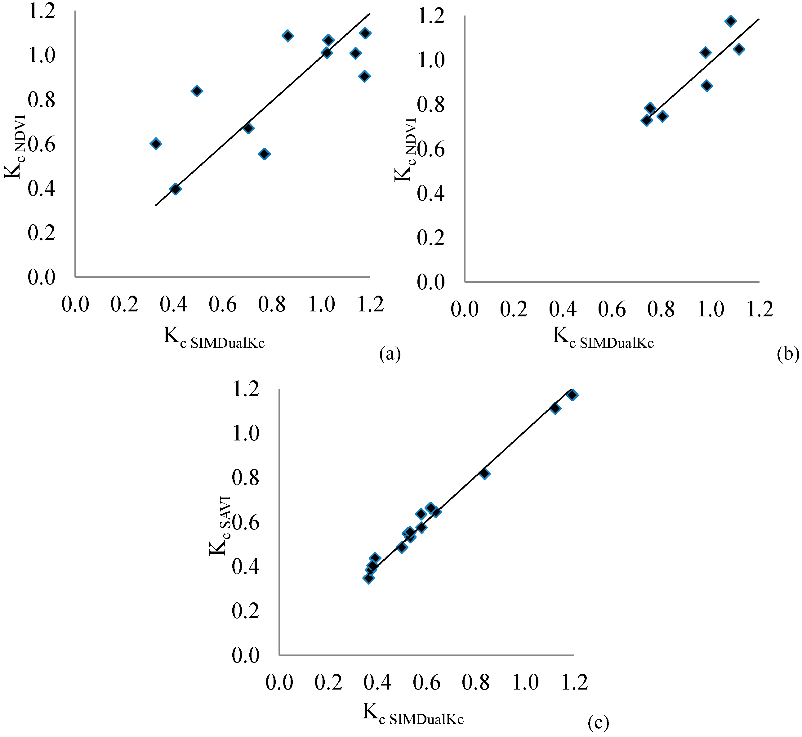
3.3. Estimation of Actual Kc from Reflectance-Based Vegetation Indices (Kc VI)
| b | R2 | n | p | Estimation | Cross Validation | |||
|---|---|---|---|---|---|---|---|---|
| RMSD ( ) | RMD (%) | RMSD ( ) | RMD (%) | |||||
| Maize | 0.99 | 0.72 | 15 | 0.0000637 | 0.16 | 12.7 | 0.08 | 6.9 |
| Barley | 0.99 | 0.83 | 7 | 0.0043194 | 0.07 | 6.4 | 0.03 | 2.6 |
| Olive | 1.01 | 0.99 | 15 | 0.0000000 | 0.02 | 3.3 | 0.01 | 2.1 |

| Crop Growth Stages | Maize | Barley | Olive |
|---|---|---|---|
| Initial | (1) | 0.78 ( ) (2) | 0.76 (±0.41) (3) |
| Development (4) | [0.90–1.30] (5) | [0.75–1.18] | [0.44–0.82] (6) |
| Mid-season | 0.98 (±0.11) (7) | 0.88 ( ) (2) | 0.62 (±0.08) (8) |
| Late-season (4) | [0.84–0.55] | [1.03–0.73] | [0.53–0.40] |
4. Discussion
4.1. Estimation of the Fraction of Ground Cover from Vegetation Indices
4.2. Estimation of Actual Kcb from Reflectance-Based Vegetation Indices (Kcb VI)
4.3. Estimation of Actual Kc by Combining Kcb VI with Ke from SIMDualKc (Kc VI)
5. Conclusions
Acknowledgments
Author Contributions
List of Symbols and Acronyms
| Dr | Root zone depletion [mm] |
| ET | Evapotranspiration [mm] |
| ETc | Crop evapotranspiration [mm] |
| ETo | Reference evapotranspiration [mm] |
| fc | Fraction of ground cover [ ] |
| fc field | Fraction of ground cover based on field data [ ] |
| fc VI | Fraction of ground cover based on vegetation indices data [ ] |
| few | Fraction of the soil that is both exposed and wetted [ ] |
| fc eff | Effective fraction of ground covered or shaded by vegetation near solar noon [ ] |
| h | Mean height of the vegetation [m] |
| Kc | Crop coefficient [ ] |
| Kc act | Actual crop coefficient [ ] |
| Kcb act | Actual basal crop coefficient [ ] |
| Kcb cover | Kcb of the ground cover in the absence of tree foliage [ ] |
| Kcb full | Estimated basal Kcb for peak plant growth conditions having nearly full ground cover [ ] |
| Kc max | Maximum value of Kc following rain or an irrigation event [ ] |
| Kc min | Minimum Kc for bare soil [ ] |
| Kc VI | Kc act computed combining the Kcb act derived from vegetation indices and the Ke derived from SIMDualKc [ ] |
| Kc NDVI | Kc act computed combining the Kcb act derived from NDVI and the Ke derived from SIMDualKc [ ] |
| Kc SAVI | Kc act computed combining the Kcb act derived from SAVI and the Ke derived from SIMDualKc [ ] |
| Kc SIMDualKc | Kc computed with SIMDualKc [ ] |
| Kcb VI | Kcb act computed from a vegetation index [ ] |
| Kcb NDVI | Kcb act computed from NDVI [ ] |
| Kcb SAVI | Kcb act computed from SAVI [ ] |
| Kcb SIMDualKc | Kcb act computed with SIMDualKc [ ] |
| Kd | Density coefficient [ ] |
| Ke | Soil evaporation coefficient [ ] |
| Kr | Evaporation reduction coefficient dependent on the cumulative depth of water depleted (evaporated) from the topsoil [ ] |
| Ks | Water stress coefficient [ ] |
| LAI | Leaf area index [m2·m−2 ] |
| ML | Multiplier on fc eff describing the effect of canopy density on shading and on maximum relative ET per fraction of ground shaded [ ] |
| p | Soil water depletion fraction for no stress [ ] |
| TAW | Total available water [mm] |
| RAW | Readily available soil water [mm] |
| RMD | Relative mean difference [%] |
| RMSD | Root-mean-square deviation [ ] |
| a.s.l | Above sea level [m] |
| ETM+ | Enhanced thematic mapper |
| NDVI | Normalized difference vegetation index |
| NIR | Near infrared |
| RS | Remote sensing |
| SAVI | Soil adjusted vegetation index |
| TM | Thematic mapper |
| VI | Vegetation index |
| VIi | VI for a specific date and pixel |
| VImax | VI for maximum vegetation cover |
| VImin | VI for minimum vegetation cover |
| β1 | Empirical coefficient depending upon the maximum NDVI value in each crop growth stage |
| β2 | Adjustment coefficient associated with crop senescence and leaves yellowing |
Conflicts of Interest
References
- Allen, R.G.; Pereira, L.S.; Raes, D.; Smith, M. Crop Evapotranspiration: Guidelines for Computing Crop Water Requirements. FAO Irrigation and Drainage Paper 56; FAO—Food and Agriculture Organization of the United Nations: Rome, Italy, 1998; p. 300. [Google Scholar]
- Monteith, J.L. Evaporation and environmen. In 19th Symposia of the Society for Experimental Biology; University Press: Cambridge, CA, USA, 1965; pp. 205–234. [Google Scholar]
- Shuttleworth, W.J.; Wallace, J.S. Calculating the water requirements of irrigated crops in Australia using the Matt-Shuttleworth approach. Trans. ASABE 2009, 52, 1895–1906. [Google Scholar] [CrossRef]
- Bastiaanssen, W.G.M.; Noordman, E.J.M.; Pelgrum, H.; Davids, G.; Thoreson, B.P.; Allen, R.G. SEBAL model with remotely sensed data to improve water-resources management under actual field conditions. J. Irrig. Drain. Eng. 2005, 131, 85–93. [Google Scholar] [CrossRef]
- Allen, R.G.; Tasumi, M.; Trezza, R. Satellite-based energy balance for mapping evapotranspiration with internalized calibration (METRIC)—Model. J. Irrig. Drain. Eng. 2007, 133, 380–394. [Google Scholar] [CrossRef]
- Kustas, W.P.; Norman, J.M.; Schmugge, T.J.; Anderson, M.C. Mapping surface energy fluxes with radiometric temperature. Chapter 7. In Thermal Remote Sensing in Land Surface Processes; Quattrochi, D., Luvall, J., Eds.; CRC Press: Boca Raton, FL, USA, 2004; pp. 205–253. [Google Scholar]
- Mateos, L.; González-Dugo, M.P.; Testi, L.; Villalobos, F.J. Monitoring evapotranspiration of irrigated crops using crop coefficients derived from time series of satellite images. I. Method validation. Agric. Water Manag. 2013, 125, 81–91. [Google Scholar] [CrossRef]
- Paço, T.A.; Pôças, I.; Cunha, M.; Silvestre, J.C.; Santos, F.L.; Paredes, P.; Pereira, L.S. Evapotranspiration and crop coefficients for a super intensive olive orchard. An application of SIMDualKc and METRIC models using ground and satellite observations. J. Hydrol. 2014, 519B, 2067–2080. [Google Scholar] [CrossRef]
- Pakparvar, M.; Cornelis, W.; Pereira, L.S.; Gabriels, D.; Hosseinimarandi, H.; Edraki, M.; Kowsar, S.A. Remote sensing estimation of actual evapotranspiration and crop coefficients for a multiple land use arid landscape of southern Iran with limited available data. J. Hydroinf. 2014, 16, 1441–1460. [Google Scholar] [CrossRef]
- Pôças, I.; Cunha, M.; Pereira, L.S.; Allen, R.G. Using remote sensing energy balance and evapotranspiration to characterize montane landscape vegetation with focus on grass and pasture lands. Int. J. Appl. Earth Obs. Geoinf. 2013, 21, 159–172. [Google Scholar] [CrossRef]
- Pereira, L.S.; Allen, R.G.; Smith, M.; Raes, D. Crop evapotranspiration estimation with FAO56: Past and future. Agric. Water Manag. 2015, 147, 4–20. [Google Scholar] [CrossRef]
- Allen, R.G.; Pereira, L.S. Estimating crop coefficients from fraction of ground cover and height. Irrig. Sci. 2009, 28, 17–34. [Google Scholar] [CrossRef]
- Campos, I.; Neale, C.M.U.; Calera, A.; Balbontín, C.; González-Piqueras, J. Assessing satellite-based basal crop coefficients for irrigated grapes (Vitis vinifera L.). Agric. Water Manag. 2010, 98, 45–54. [Google Scholar] [CrossRef]
- Calera, A.; Jochum, A.M.; GarcÍa, A.C.; Rodríguez, A.M.; Fuster, P.L. Irrigation management from space: Towards user-friendly products. Irrig. Drain. Syst. 2005, 19, 337–353. [Google Scholar] [CrossRef]
- Allen, R.G.; Tasumi, M.; Morse, A.; Trezza, R.; Wright, J.L.; Bastiaanssen, W.; Kramber, W.; Lorite, I.; Robison, C.W. Satellite-based energy balance for mapping evapotranspiration with internalized calibration (METRIC)—Applications. J. Irrig. Drain. Eng. 2007, 133, 395–406. [Google Scholar] [CrossRef]
- Glenn, E.P.; Huete, A.R.; Nagler, P.L.; Nelson, S.G. Relationship between remotely-sensed vegetation indices, canopy attributes and plant physiological processes: What vegetation indices can and cannot tell us about the landscape. Sensors 2008, 8, 2136–2160. [Google Scholar] [CrossRef]
- Glenn, E.P.; Neale, C.M.U.; Hunsaker, D.J.; Nagler, P.L. Vegetation index-based crop coefficients to estimate evapotranspiration by remote sensing in agricultural and natural ecosystems. Hydrol. Process. 2011, 25, 4050–4062. [Google Scholar] [CrossRef]
- Johnson, L.F.; Trout, T.J. Satellite NDVI assisted monitoring of vegetable crop evapotranspiration in California’s San Joaquin valley. Remote Sens. 2012, 4, 439–455. [Google Scholar] [CrossRef]
- Viña, A.; Gitelson, A.A.; Nguy-Robertson, A.L.; Peng, Y. Comparison of different vegetation indices for the remote assessment of green leaf area index of crops. Remote Sens. Environ. 2011, 115, 3468–3478. [Google Scholar] [CrossRef]
- Hunsaker, D.; Pinter, P.J., Jr.; Kimball, B. Wheat basal crop coefficients determined by normalized difference vegetation index. Irrig. Sci. 2005, 24, 1–14. [Google Scholar] [CrossRef]
- Allen, R.G.; Pereira, L.S.; Howell, T.A.; Jensen, M.E. Evapotranspiration information reporting: I. Factors governing measurement accuracy. Agric. Water Manag. 2011, 98, 899–920. [Google Scholar] [CrossRef]
- Rouse, W.; Haas, R.; Scheel, J.; Deering, W. Monitoring Vegetation Systems in Great Plains with ERTS. In Proceedings of the Third ERTS Symposium, NASA SP-351, Washington, DC, USA, 10–14 December 1973; US Government Printing Office: Washington, DC, USA, 1973; pp. 309–317. [Google Scholar]
- Huete, A.R. A soil-adjusted vegetation index (SAVI). Remote Sens. Environ. 1988, 25, 295–309. [Google Scholar] [CrossRef]
- Jensen, J.R. Remote Sensing of Environment. An Earth Resource Perspective; Prentice Hall, Inc.: Upper Saddle River, NJ, USA, 2000. [Google Scholar]
- Choudhury, B.J.; Ahmed, N.U.; Idso, S.B.; Reginato, R.J.; Daughtry, C.S.T. Relations between evaporation coefficients and vegetation indices studied by model simulations. Remote Sens. Environ. 1994, 50, 1–17. [Google Scholar] [CrossRef]
- Jayanthi, H.; Neale, C.M.U.; Wright, J.L. Development and validation of canopy reflectance-based crop coefficient for potato. Agric. Water Manag. 2007, 88, 235–246. [Google Scholar] [CrossRef]
- Hunsaker, D.J.; Pinter, P.J., Jr.; Barnes, E.M.; Kimball, B.A. Estimating cotton evapotranspiration crop coefficients with a multispectral vegetation index. Irrig. Sci. 2003, 22, 95–104. [Google Scholar] [CrossRef]
- Bausch, W.C.; Neale, C.M.U. Crop coefficients derived from reflected canopy radiation: A concept. Trans. ASAE 1987, 30, 703–709. [Google Scholar] [CrossRef]
- Er-Raki, S.; Rodriguez, J.C.; Garatuza-Payan, J.; Watts, C.J.; Chehbouni, A. Determination of crop evapotranspiration of table grapes in a semi-arid region of Northwest Mexico using multi-spectral vegetation index. Agric. Water Manag. 2013, 122, 12–19. [Google Scholar] [CrossRef]
- Er-Raki, S.; Chehbouni, A.; Guemouria, N.; Duchemin, B.; Ezzahar, J.; Hadria, R. Combining FAO-56 model and ground-based remote sensing to estimate water consumptions of wheat crops in a semi-arid region. Agric. Water Manag. 2007, 87, 41–54. [Google Scholar] [CrossRef]
- Padilla, F.L.M.; González-Dugo, M.P.; Gavilán, P.; Domínguez, J. Integration of vegetation indices into a water balance model to estimate evapotranspiration of wheat and corn. Hydrol. Earth Syst. Sci. 2011, 15, 1213–1225. [Google Scholar] [CrossRef]
- Rosa, R.D.; Paredes, P.; Rodrigues, G.C.; Alves, I.; Fernando, R.M.; Pereira, L.S.; Allen, R.G. Implementing the dual crop coefficient approach in interactive software. 1. Background and computational strategy. Agric. Water Manag. 2012, 103, 8–24. [Google Scholar] [CrossRef]
- Pôças, I.; Paço, T.A.; Cunha, M.; Andrade, J.A.; Silvestre, J.; Sousa, A.; Santos, F.L.; Pereira, L.S.; Allen, R.G. Satellite based evapotranspiration of a super-intensive olive orchard: Application of METRIC algorithms. Biosyst. Eng. 2014, 126, 69–81. [Google Scholar] [CrossRef]
- Paredes, P.; Rodrigues, G.C.; Alves, I.; Pereira, L.S. Partitioning evapotranspiration, yield prediction and economic returns of maize under various irrigation management strategies. Agric. Water Manag. 2014, 135, 27–39. [Google Scholar] [CrossRef]
- Pereira, L.S.; Paredes, P.; Rodrigues, G.C.; Neves, M. Modeling malt barley water use and evapotranspiration partitioning in two contrasting rainfall years. Assessing AquaCrop and SIMDualKc models. Agric. Water Manag. 2015. submitted. [Google Scholar]
- Tasumi, M.; Allen, R.G.; Trezza, R. At-surface reflectance and albedo from satellite for operational calculation of land surface energy balance. J. Hydrol. Eng. 2008, 13, 51–63. [Google Scholar] [CrossRef]
- Chander, G.; Markham, B.L.; Helder, D.L. Summary of current radiometric calibration coefficients for Landsat MSS, TM, ETM+, and EO-1 ALI sensors. Remote Sens. Environ. 2009, 113, 893–903. [Google Scholar] [CrossRef]
- Chander, G.; Markham, B. Revised Landsat-5 TM radiometric calibration procedures and postcalibration dynamic ranges. IEEE Trans. Geosci. Remote Sens. 2003, 41, 2674–2677. [Google Scholar] [CrossRef]
- Rosa, R.D.; Paredes, P.; Rodrigues, G.C.; Fernando, R.M.; Alves, I.; Pereira, L.S.; Allen, R.G. Implementing the dual crop coefficient approach in interactive software: 2. Model testing. Agric. Water Manag. 2012, 103, 62–77. [Google Scholar] [CrossRef]
- Paço, T.; Ferreira, M.; Rosa, R.; Paredes, P.; Rodrigues, G.; Conceição, N.; Pacheco, C.; Pereira, L. The dual crop coefficient approach using a density factor to simulate the evapotranspiration of a peach orchard: SIMDualKc model versus eddy covariance measurements. Irrig. Sci. 2012, 30, 115–126. [Google Scholar] [CrossRef]
- Ding, R.; Kang, S.; Zhang, Y.; Hao, X.; Tong, L.; Du, T. Partitioning evapotranspiration into soil evaporation and transpiration using a modified dual crop coefficient model in irrigated maize field with ground-mulching. Agric. Water Manag. 2013, 127, 85–96. [Google Scholar] [CrossRef]
- Phogat, V.; Skewes, M.A.; Mahadevan, M.; Cox, J.W. Evaluation of soil plant system response to pulsed drip irrigation of an almond tree under sustained stress conditions. Agric. Water Manag. 2013, 118, 1–11. [Google Scholar] [CrossRef]
- Santos, C.; Lorite, I.J.; Allen, R.G.; Tasumi, M. Aerodynamic Parameterization of the Satellite-Based Energy Balance (METRIC) Model for ET Estimation in Rainfed Olive Orchards of Andalusia, Spain. Water Resour. Manag. 2012, 26, 3267–3283. [Google Scholar] [CrossRef]
- Allen, R.G.; Pereira, L.S.; Smith, M.; Raes, D.; Wright, J. FAO-56 dual crop coefficient method for estimating evaporation from soil and application extensions. J. Irrig. Drain. Eng. 2005, 131, 2–13. [Google Scholar] [CrossRef]
- Zhao, N.; Liu, Y.; Cai, J.; Paredes, P.; Rosa, R.D.; Pereira, L.S. Dual crop coefficient modeling applied to the winter wheat—Summer maize crop sequence in North China Plain: Basal crop coefficients and soil evaporation component. Agric. Water Manag. 2013, 117, 93–105. [Google Scholar] [CrossRef]
- Wei, Z.; Paredes, P.; Liu, Y.; Chi, W.W.; Pereira, L.S. Modeling transpiration, soil evaporation and yield prediction of soybean in North China Plain. Agric. Water Manag. 2015, 147, 43–53. [Google Scholar] [CrossRef]
- Zhang, B.; Liu, Y.; Xu, D.; Zhao, N.; Lei, B.; Rosa, R.D.; Paredes, P.; Paço, T.A.; Pereira, L.S. The dual crop coefficient approach to estimate and partitioning evapotranspiration of the winter wheat—summer maize crop sequence in North China Plain. Irrig. Sci. 2013, 31, 1303–1316. [Google Scholar] [CrossRef]
- Calera Belmonte, A.; Jochum, A.M.; García, A.C. Space-assisted irrigation management: Towards user-friendly products. In Proceedings of ICID Workshop on Use of Remote Sensing of Crop Evapotranspiration for Large Regions, Montpellier, France, 17 September 2003.
- Calera, A.; González-Piqueras, J.; Melia, J. Monitoring barley and corn growth from remote sensing data at field scale. Int. J. Remote Sens. 2004, 25, 97–109. [Google Scholar] [CrossRef]
- Duchemin, B.; Hadria, R.; Erraki, S.; Boulet, G.; Maisongrande, P.; Chehbouni, A.; Escadafal, R.; Ezzahar, J.; Hoedjes, J.C.B.; Kharrou, M.H.; et al. Monitoring wheat phenology and irrigation in Central Morocco: On the use of relationships between evapotranspiration, crops coefficients, leaf area index and remotely-sensed vegetation indices. Agric. Water Manag. 2006, 79, 1–27. [Google Scholar] [CrossRef]
- González-Dugo, M.P.; Mateos, L. Spectral vegetation indices for benchmarking water productivity of irrigated cotton and sugarbeet crops. Agric. Water Manag. 2008, 95, 48–58. [Google Scholar] [CrossRef]
- Stagakis, S.; González-Dugo, V.; Cid, P.; Guillén-Climent, M.L.; Zarco-Tejada, P.J. Monitoring water stress and fruit quality in an orange orchard under regulated deficit irrigation using narrow-band structural and physiological remote sensing indices. ISPRS J. Photogramm. Remote Sens. 2012, 71, 47–61. [Google Scholar] [CrossRef]
- Kohavi, R. A study of cross-validation and bootstrap for accuracy estimation and model selection. In Proceedings of the Fourteenth International Joint Conference on Artificial Intelligence, Montreal Quebec, Canada, 20–25 August, 1995; Morgan Kaufman Publishers Inc.: San Francisco, CA, USA; pp. 1137–1143.
- Cunha, M.; Marçal, A.R.S.; Silva, L. Very early prediction of wine yield based on satellite data from VEGETATION. Int. J. Remote Sens. 2010, 31, 3125–3142. [Google Scholar] [CrossRef]
- Lindberg, E.; Holmgren, J.; Olofsson, K.; Wallerman, J.; Olsson, H. Estimation of tree lists from airborne laser scanning using tree model clustering and k-MSN imputation. Remote Sens. 2013, 5, 1932–1955. [Google Scholar] [CrossRef]
- Trout, T.J.; Johnson, L.F.; Gartung, J. Remote sensing of canopy cover in horticultural crops. HortScience 2008, 43, 333–337. [Google Scholar]
- Purevdorj, T.S.; Tateishi, R.; Ishiyama, T.; Honda, Y. Relationships between percent vegetation cover and vegetation indices. Int. J. Remote Sens. 1998, 19, 3519–3535. [Google Scholar] [CrossRef]
- Carreiras, J.M.B.; Pereira, J.M.C.; Pereira, J.S. Estimation of tree canopy cover in evergreen oak woodlands using remote sensing. For. Ecol. Manag. 2006, 223, 45–53. [Google Scholar] [CrossRef]
- Gonzalez-Piqueras, J.; Calera Belmonte, A.; Gilabert, M.A.; Cuesta García, A.; de la Cruz Tercero, F. Estimation of crop coefficient by means of optimized vegetation indices for corn. Proc. SPIE 2004, 5232. [Google Scholar] [CrossRef]
- Bausch, W.C. Soil background effects on reflectance-based crop coefficients for corn. Remote Sens. Environ. 1993, 46, 213–222. [Google Scholar] [CrossRef]
- Hunsaker, D.J.; Fitzgerald, G.J.; French, A.N.; Clarke, T.R.; Ottman, M.J.; Pinter, P.J., Jr. Wheat irrigation management using multispectral crop coefficients: I. Crop evapotranspiration prediction. Trans. ASAE 2007, 50, 2017–2033. [Google Scholar] [CrossRef]
- Liu, Z.; Yao, Z.; Yu, C.; Zhong, Z. Assessing crop water demand and deficit for the growth of spring highland barley in Tibet, China. J. Integr. Agric. 2013, 12, 541–551. [Google Scholar] [CrossRef]
- Villalobos, F.J.; Orgaz, F.; Testi, L.; Fereres, E. Measurement and modeling of evapotranspiration of olive (Olea europaea L.) orchards. Eur. J. Agron. 2000, 13, 155–163. [Google Scholar] [CrossRef]
© 2015 by the authors; licensee MDPI, Basel, Switzerland. This article is an open access article distributed under the terms and conditions of the Creative Commons Attribution license (http://creativecommons.org/licenses/by/4.0/).
Share and Cite
Pôças, I.; Paço, T.A.; Paredes, P.; Cunha, M.; Pereira, L.S. Estimation of Actual Crop Coefficients Using Remotely Sensed Vegetation Indices and Soil Water Balance Modelled Data. Remote Sens. 2015, 7, 2373-2400. https://doi.org/10.3390/rs70302373
Pôças I, Paço TA, Paredes P, Cunha M, Pereira LS. Estimation of Actual Crop Coefficients Using Remotely Sensed Vegetation Indices and Soil Water Balance Modelled Data. Remote Sensing. 2015; 7(3):2373-2400. https://doi.org/10.3390/rs70302373
Chicago/Turabian StylePôças, Isabel, Teresa A. Paço, Paula Paredes, Mário Cunha, and Luís S. Pereira. 2015. "Estimation of Actual Crop Coefficients Using Remotely Sensed Vegetation Indices and Soil Water Balance Modelled Data" Remote Sensing 7, no. 3: 2373-2400. https://doi.org/10.3390/rs70302373