Article

An Optimal Sampling Design for Observing and Validating Long-Term Leaf Area Index with Temporal Variations in Spatial Heterogeneities

1
State Key Laboratory of Remote Sensing Science, Institute of Remote Sensing and Digital Earth, Chinese Academy of Sciences, No. 20A, Datun Road, Chaoyang District, Beijing 100101, China
2
College of Resources and Environment, University of Chinese Academy of Sciences, Beijing 100049, China
3
Joint Center for Global Change Studies, Beijing 100875, China
4
Plant Functional Biology and Climate Change Cluster (C3), University of Technology, Sydney 2007, Australia
*
Authors to whom correspondence should be addressed.
Remote Sens. 2015, 7(2), 1300-1319; https://doi.org/10.3390/rs70201300
Submission received: 17 October 2014 / Revised: 17 October 2014 / Accepted: 15 January 2015 / Published: 26 January 2015

Abstract

:
A sampling strategy to define elementary sampling units (ESUs) for an entire site at the kilometer scale is an important step in the validation process for moderate-resolution leaf area index (LAI) products. Current LAI-sampling strategies are unable to consider the vegetation seasonal changes and are better suited for single-day LAI product validation, whereas the increasingly used wireless sensor network for LAI measurement (LAINet) requires an optimal sampling strategy across both spatial and temporal scales. In this study, we developed an efficient and robust LAI Sampling strategy based on Multi-temporal Prior knowledge (SMP) for long-term, fixed-position LAI observations. The SMP approach employed multi-temporal vegetation index (VI) maps and the vegetation classification map as a priori knowledge. The SMP approach minimized the multi-temporal bias of the VI frequency histogram between the ESUs and the entire site and maximized the nearest-neighbor index to ensure that ESUs were dispersed in the geographical space. The SMP approach was compared with four sampling strategies including random sampling, systematic sampling, sampling based on the land-cover map and a sampling strategy based on vegetation index prior knowledge using the PROSAIL model-based simulation analysis in the Heihe River basin. The results indicate that the ESUs selected using the SMP method spread more evenly in both the multi-temporal feature space and geographical space over the vegetation cycle. By considering the temporal changes in heterogeneity, the average root-mean-square error (RMSE) of the LAI reference maps can be reduced from 0.12 to 0.05, and the relative error can be reduced from 6.1% to 2.2%. The SMP technique was applied to assign the LAINet ESU locations at the Huailai Remote Sensing Experimental Station in Beijing, China, from 4 July to 28 August 2013, to validate three MODIS C5 LAI products. The results suggest that the average R2, RMSE, bias and relative uncertainty for the three MODIS LAI products were 0.60, 0.33, −0.11, and 12.2%, respectively. The MCD15A2 product performed best, exhibiting a RMSE of 0.20, a bias of −0.07 and a relative uncertainty of 7.4%. Future efforts are needed to obtain more long-term validation datasets using the SMP approach on different vegetation types for validating moderate-resolution LAI products in time series.

Graphical Abstract

1. Introduction

The leaf area index (LAI) is defined as half of the total foliage area per unit ground surface area [1,2]. The LAI is an important biophysical variable in land-surface processes, such as photosynthesis, transpiration and energy balance [3]. Several remotely sensed global LAI products have been produced from multiple sensors, such as TERRA and AQUA/MODIS, SPOT/VEGETATION, ENVISAT/MERIS, TERRA/MISR and AVHRR [4,5,6,7,8,9]. Ground-based validation is critical for assessing the uncertainties and evaluating the accuracies of these satellite-derived products [10,11,12,13]. In the general “bottom-up” products validation framework, selection of the sampling strategy to define elementary sampling units (ESUs) for the entire site at the kilometer scale is an important step because the chosen sampling strategy results in different coefficients of the up-scaling function that ultimately affect the accuracy assessment of the LAI product [13,14,15]. The widely used random sampling or systematic sampling approaches in prior validation programs are simple and easy to carry out [16,17,18,19], but these approaches may not be appropriate over heterogeneous areas due to their low efficiency and the laborious and time-consuming nature of LAI field measurements [20]. To capture the surface heterogeneity, more efficient sampling strategies are designed with available a priori knowledge, such as vegetation types, vegetation index or soil types [21,22,23,24]. These methods are widely applied in the VALERI project field campaigns, the Ruokolahti forest observations in Finland and the Barrax cropland observations in Spain [25,26,27].
To study the seasonal variation of vegetation growth, much attention has recently been paid to the continuous observing of LAI time series and the long-term multi-temporal validation of LAI products [28,29,30]. The wireless sensor network (WSN) designed for LAI measurement (LAINet) provides a feasible and efficient scheme for continuous LAI observing from in-situ downward solar radiation and transmitted radiation measurements [31,32]. The LAINet has the potential to continuously monitor temporal variability in harsh conditions, such as at high altitudes or in cold temperatures, and is increasingly being used in ground observation programs [31,32,33,34,35]. Due to budget constraints, the number of LAINet nodes for an observation area is typically fixed. Therefore, the main freedom is the choice of locations for the LAINet nodes. Once established, the node locations are typically fixed for performing continuous observations [30]. Thus, the sampling strategy for the assignment of LAINet nodes requires optimization for the entire observation period, rather than for a specific or short observation period. One of the limitations of the currently employed LAI sampling strategies is that they are not designed for extended dynamic vegetation growth and are better suited for single-day LAI product validation. It is necessary to account for surface temporal changes to achieve the optimal sampling across both spatial and temporal scales.
The objective of this study is to introduce the temporal domain into the sampling strategy for observing long-term LAI with temporal changes in spatial heterogeneities. The proposed sampling strategy employs multiple species and multi-temporal a priori information. This paper is organized as follows. Section 2 describes the methodology of the Sampling strategy based on Multi-temporal Prior knowledge (SMP) and the sampling strategy evaluation procedure. The study sites and the data processing procedure are described in Section 3. In Section 4, the SMP method is compared with four alternate sampling strategies using the PROSAIL model-based simulation analysis in the Heihe River basin, and Section 4 also presents the application of the SMP method in the LAINet observations at the Huailai Remote Sensing Experimental Station in Beijing, China, from 4 July to 28 August 2013. Finally, conclusions and directions for needed future research on the SMP method are presented in Section 5.

2. Methodology

2.1. Sampling Strategy Based on Multi-Temporal a Priori Knowledge

The LAINet within an ESU (~30 m) contains three different types of sub-nodes: one to multiple evenly distributed “below” sub-nodes, which are deployed below the canopy to receive the transmitted solar radiation; one “above” sub-node, which is above the canopy to receive the downward radiation; and one central sub-node, which is used for data reception and control. Each below sub-node calculates the LAI from multi-angle transmittance using a vegetation gap probability model, and all the below sub-node observations within an ESU are averaged as the field-measured LAI value of the ESU. In general, the site-specific relationship (transfer function) between the field-measured LAI of each ESU and fine-resolution VI values is either a univariate exponential or a linear regression function. The goal of proposing an optimal sampling strategy for validating LAI products in time series is to improve the accuracy of the multi-temporal LAI reference maps at the given number of ESUs.
The feature space, or attribute space, is a virtual space bounded by the range of variables [36]. The axes of the feature space include continuous variables such as the vegetation index and categorical variables such as the land-cover types. The SMP method is designed to ensure the even spread of ESUs in both multi-temporal feature space and geographical space, and the objective function (OF) is defined as follows:
OF = Bias Total / NNI
where NNI is the nearest neighbor index which is given in Equation (5), and BiasTotal is defined as follows:
Bias Total = Bias VI + Bias LC
where BiasVI is the multi-temporal average bias between the VI frequency distribution histogram of the ESUs and the entire site and is given by the following relation:
Bias VI = t = 1 T i = 1 n | η ( q i ( t ) x ( t ) < q i + 1 ( t ) n 1 n |
where n is the number of ESUs, and t is the number of the corresponding multi-temporal vegetation index (VI) maps. The entire site contains N fine-resolution pixels. X (N × T) is the population of multi-temporal VI values, while x (n × T) is the group of ESUs selected from X. The frequency distribution histogram of X is divided into n intervals, and each interval has an equal number of pixels. The quantiles are defined as q 1 ( t ) , , q i ( t ) , , q n + 1 ( t ) , where t = 1, …, T, and i = 1, …, n + 1. η ( q i ( t ) x ( t ) < q i + 1 ( t ) ) is the number of times that x j appears in the interval [ q i ( t ) ,   q i + 1 ( t ) ].
BiasLC is the bias between the land-cover histogram of the ESUs and the entire site and is calculated as follows:
Bias LC = j = 1 c | η ( x j ) n κ j |
where η ( x j ) is the number of times x occurs in class j in the sampled pixels, κ j is the proportion of class j in X, and c is the number of land-cover classes.
NNI represents the nearest neighbor index and is computed as follows [37]:
NNI = i = 1 n m i n ( d i j ) n 0.5 A / n
where min(dij) is the distance between each ESU and its nearest neighbor, n is the number of ESUs, and A is the area of the site. The NNI is one of the most widely used distance statistics in the point pattern-distribution analysis [37] and has been used as a good indicator to measure the dispersion of the ESUs over the entire site in the SSVIP approach [24]. The dispersal of the ESUs spatial distribution increases with increasing values of NNI. The NNI is equal to one when the ESUs spatial distribution is random. An NNI value less than one indicates spatial aggregation, whereas a value greater than one indicates a dispersed distribution.
The six necessary steps for applying the SMP method are as follows:
(1)
Acquire multi-temporal VI images and the vegetation classification map from historical a priori knowledge.
Multi-temporal VI maps and the vegetation classification map can be acquired from fine-resolution multi-spectral images at the same period in recent history. The required number of multi-temporal VI maps depends on the changes in heterogeneity over the entire sampling period. If the temporal changes in the surface heterogeneity are continuous, three fine-resolution VI maps properly distributed over the green-up, maturity and senescence periods are generally sufficient for agricultural fields. If the heterogeneity exhibits more temporal changes, the VI maps from each time interval when the changes occur are required to ensure the representativeness of the ESUs for this time interval. The Normalized Difference Vegetation Index (NDVI), Simple Ratio (SR), or Enhanced Vegetation Index (EVI), which is sensitive to the vegetation growth levels for the specific area, can be employed.
The use of historical knowledge to guide the LAI sampling requires that the inter-annual change in vegetation growth is not as significant as the seasonal variability, which is more reasonable for natural vegetation and cropland with no sudden changes in tillage management according to the vegetation phenology [38,39]. The application of this approach will be limited if the vegetation has high abnormal inter-annual variations due to water shortages or crop species changes, etc.
(2)
Randomly select a group of n ESUs from all the fine-resolution pixels of the entire site.
(3)
Calculate the OF for the group of ESUs based on Equations (1)–(5).
(4)
Start the simulated annealing algorithm to search for the optimal group of ESUs.
To avoid being trapped in local optimum, the simulated annealing algorithm accepts some of the changes that worsen the OF, and the probability of accepting a worse group of ESUs is given by the following relation [22]:
P = exp ( ∆OF / T )
where ∆OF is the change in OF between two iterations, and T is the cooling temperature which starts at 1 and is decreased by a factor of 0.95 at every ten iterations. The process then generates a random number R between 0 and 1. If R < P, the new group of ESUs is accepted, and otherwise, the change is discarded.
(5)
Perform the change of an ESU in the group.
For the change, if R < 0.5, an ESU in the group is randomly swapped with a random ESU outside the group. Otherwise, one of the ESUs from x in Equation (3) which has the largest η ( q i ( t ) x ( t ) < q i + 1 ( t ) ) is randomly selected and replaced by a random ESU outside the group.
(6)
Repeat steps (3)–(5) until the OF value falls beyond the given stopping criterion OF < 0.01, or the defined maximum number of iterations 10,000 is reached.
Theoretically, there exists the extreme case in which more than one group of ESUs may have the same minimum OF, and in this case, one of these groups will be randomly selected as the optimal group of ESUs using the SMP method.

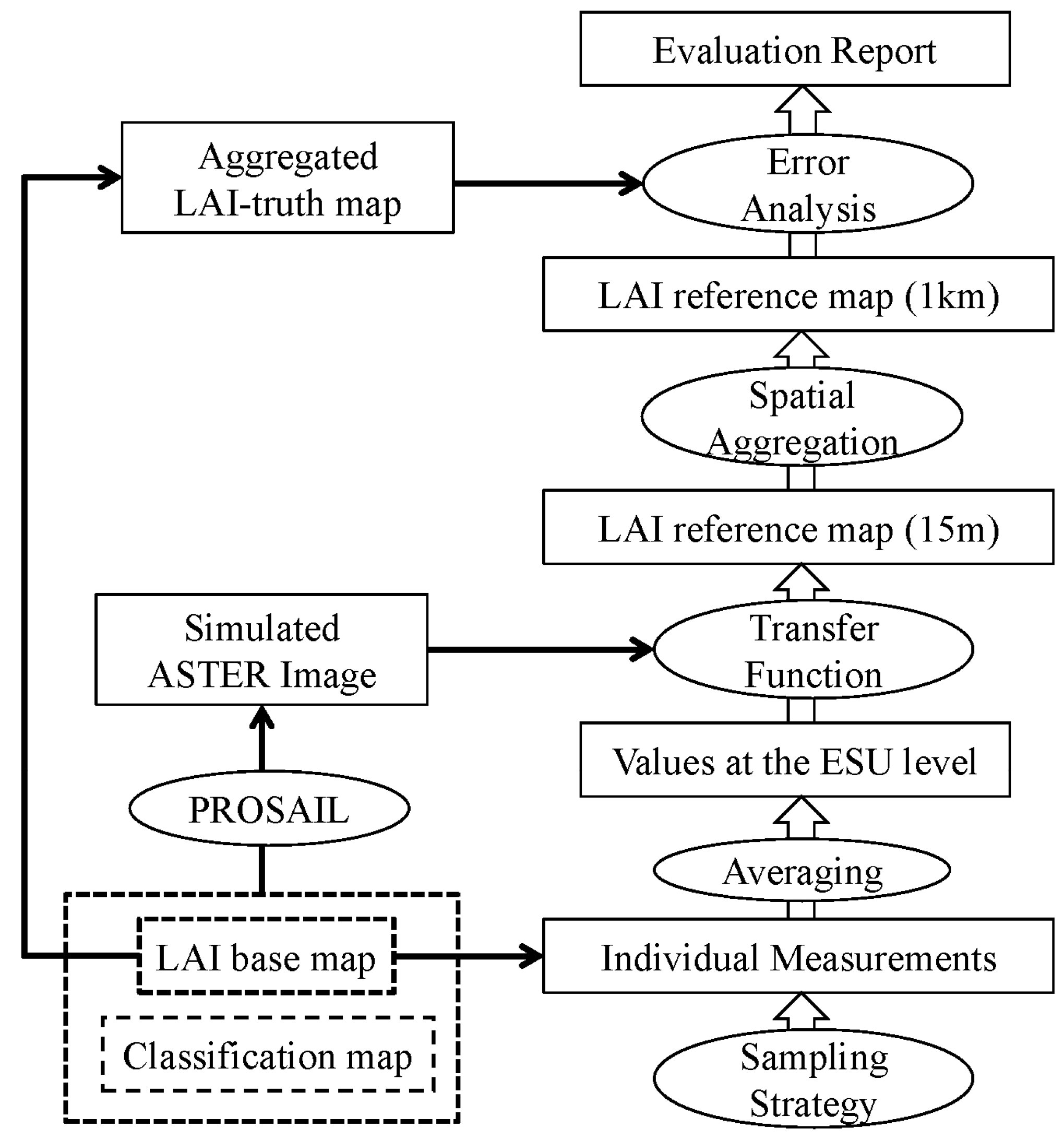
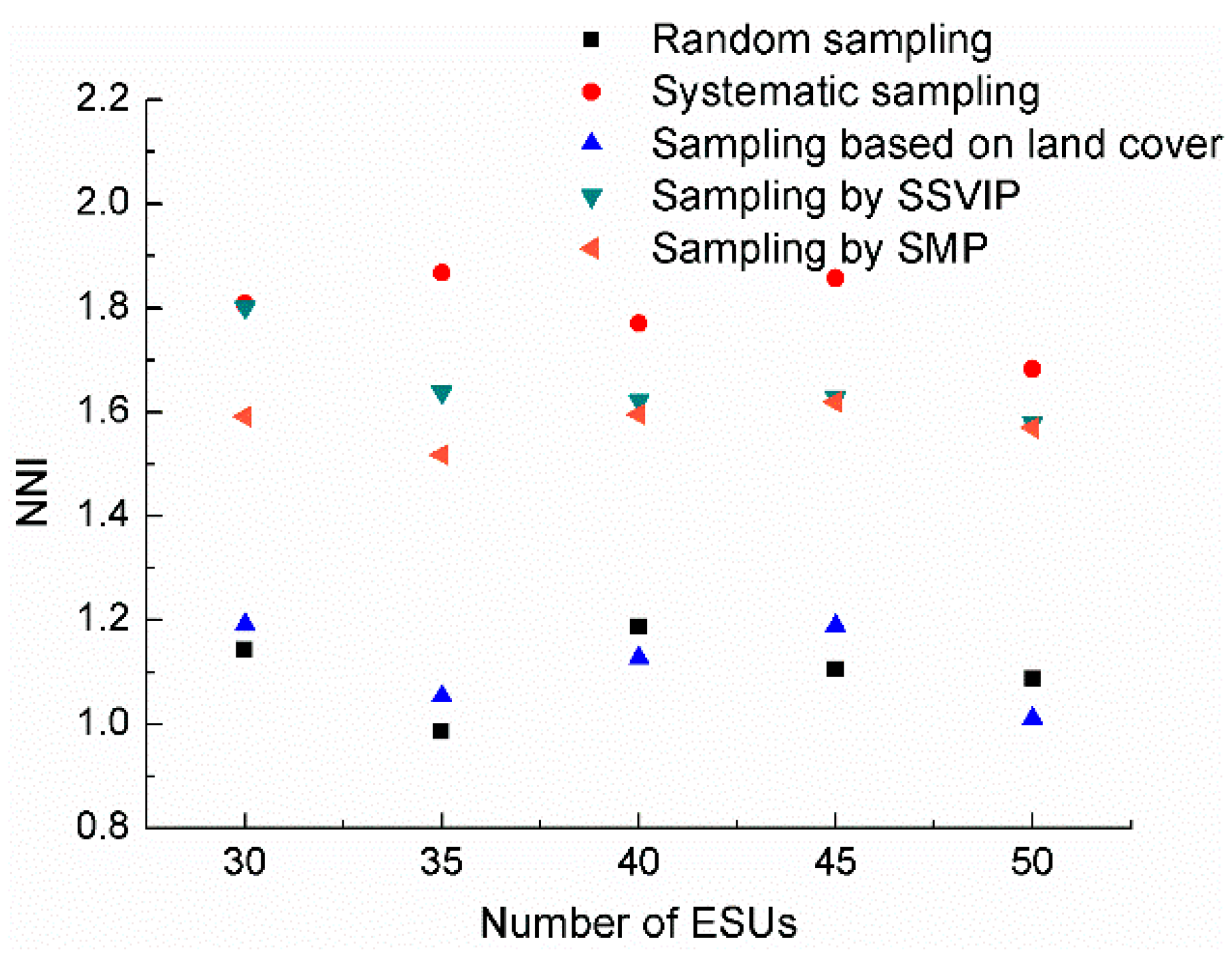
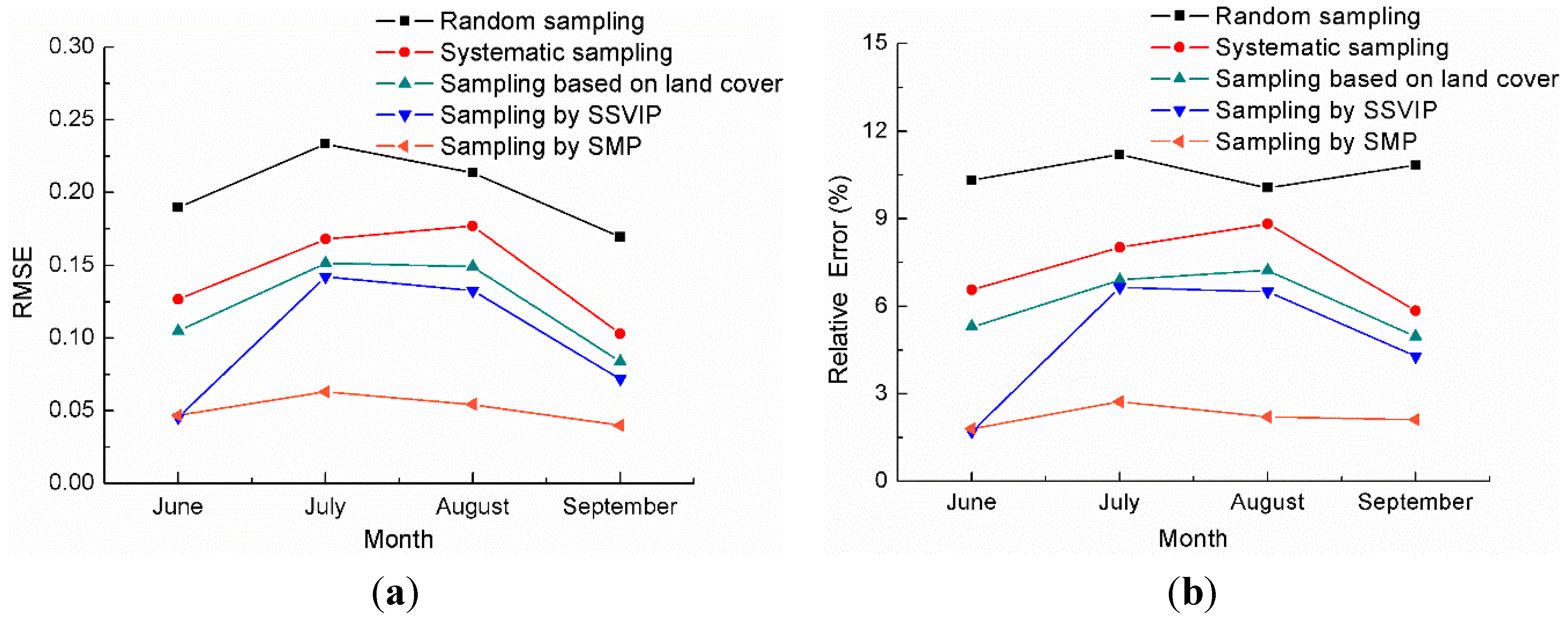
2.2. Sampling Strategy Evaluation Procedure

Directly validating the accuracy of a sampling strategy is challenging because the true LAI value of the entire study area can seldom be obtained in practice due to the limited manpower. To ensure that the true LAI values and the spectral images were simultaneously available, the direct evaluation procedure proposed by Zeng, et al. [24] was adopted here (Figure 1). This procedure was based on the PROSAIL model with a “bottom-up” LAI product-validation process [14], and the simulated images had to be similar to the satellite images in the vegetation structure and growth seasonal cycle.
In the proposed evaluation procedure, the PROSAIL model required multi-temporal fine-resolution LAI base maps and a vegetation classification map to simulate multi-temporal fine-resolution reflectance images. The LAI base maps were considered to provide the true LAI values for evaluating the accuracy of the different sampling strategies. Different sampling strategies were applied and resulted in different transfer functions that ultimately generated different LAI reference maps. The LAI of the non-vegetated areas, such as roads, buildings and bare soil, was set as zero in the LAI reference maps. The LAI reference maps were degraded to a moderate resolution to compare with the original LAI base map. The only difference among the evaluation procedures was the sampling strategy. Therefore, the accuracy of the different sampling strategies can be evaluated based on the accuracy of the multi-temporal LAI reference maps. The SMP method was compared with four current widely used sampling strategies: random sampling, systematic sampling, sampling based on the land-cover map and Sampling Strategy based on Vegetation Index Prior knowledge (SSVIP). For all the sampling strategies, non-vegetated areas were masked in the sampling. For simple random sampling, the ESU locations were selected using a series of random numbers. For systematic sampling, a series of rectangular grids were generated, and the ESU locations were chosen in the center of each grid. For sampling based on the land-cover map, the number of ESUs in each vegetation type was proportionally allocated according to the area, and the ESUs were randomly distributed within each type. For the SSVIP approach, only the first fine-resolution VI map was used as a priori knowledge. This approach was in fact a type of stratified sampling, and the number of strata for SSVIP was set equal to the number of ESUs to achieve the maximal stratification [24]. For the SMP sampling strategy, all the acquired fine-resolution VI maps during the observation periods and the land-cover map were incorporated as the input dataset to generate the optimal group of ESUs.
Figure 1. Sampling strategy evaluation framework based on the PROSAIL model [24].
Remotesensing 07 01300 g001

3. Study Sites and Data Processing

The different sampling strategies were evaluated and compared over a 3 km × 3 km agricultural area in the Heihe River basin, Gansu province, China (38°51′N, 100°21′E), and then, the proposed SMP approach was applied to select the optimal group of ESUs for the LAINet at the Huailai Remote Sensing Experimental Station (40°22′N, 115°46′E) in Beijing, China, from July to August in 2013.

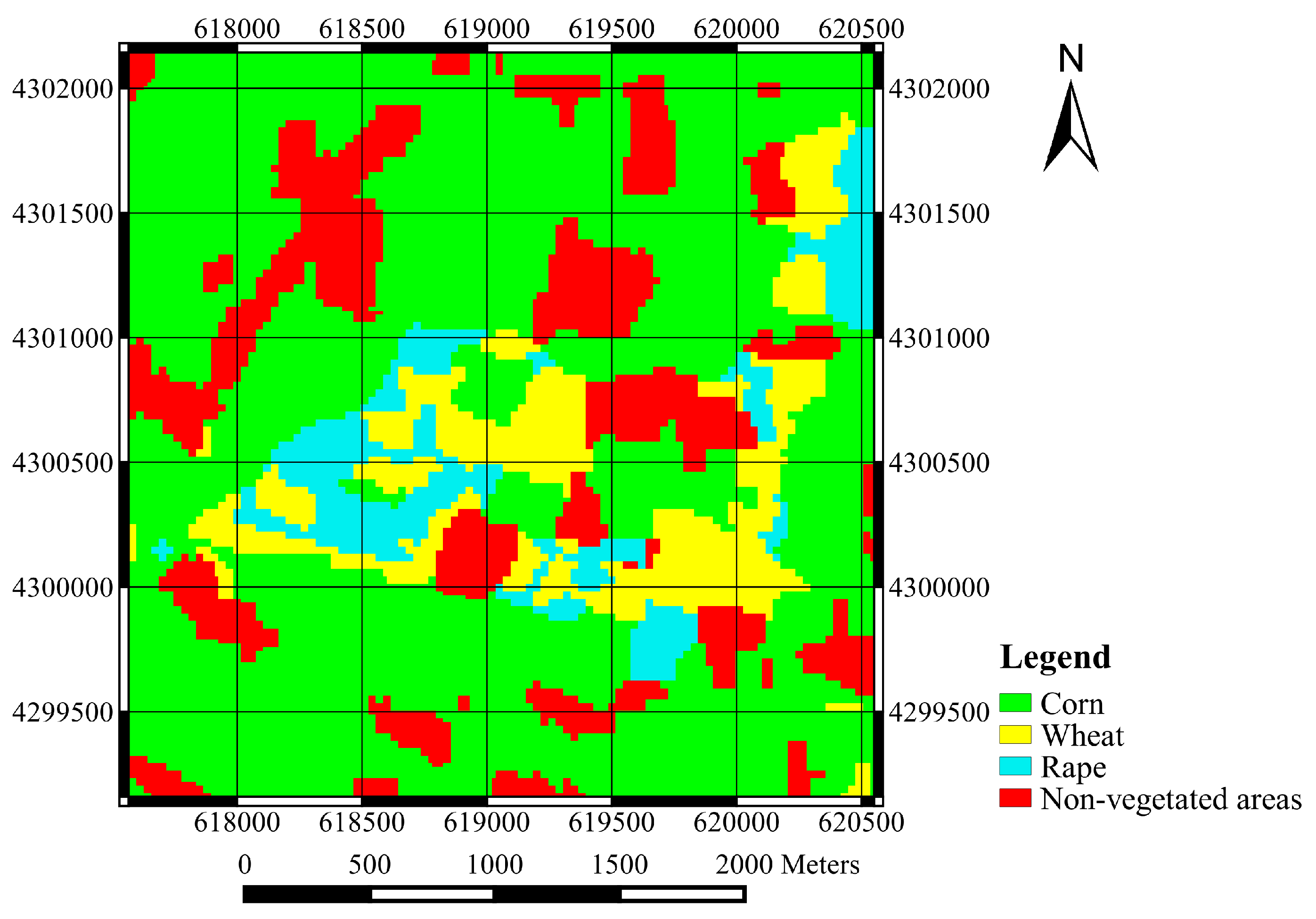
3.1. Data Acquired and Processed for the Sampling Strategy Evaluation

The vegetation classification map of the Heihe site was obtained using a supervised classification method of an HJ-1/CCD image and the ground-observed cover types of typical objects, as shown in Figure 2. The proportions of corn, wheat and rape were 76.8%, 13.7% and 9.5%, respectively. All non-vegetated areas, such as roads, buildings, and bare soil, were masked in the sampling, and thus, no ESUs are located on these areas. Four 15-m resolution ASTER images acquired on 24 June, 10 July, 11 August, and 12 September 2012, were used as the historical a priori knowledge to guide the sampling design during the growing season from June to September 2013. All images in this study were radiance calibrated and atmospherically corrected using the 6S model [40] and were previously geometrically corrected with the spatial error controlled within 0.5 pixels.
Figure 2. The land-cover map of the 3 km × 3 km study area in the Heihe River basin, China. The major cover types were corn (green), wheat (yellow), rape (cyan) and non-vegetated areas (red). The projection is UTM 47 North, WGS84.
Remotesensing 07 01300 g002
At the Heihe site, 14 ESUs were field measured by LAI-2000 on 13 July 2012, which included 11 corn ESUs, two wheat ESUs and one rape ESU. The size of the ESU was 15 m × 15 m, and nine single points measured by LAI-2000 were evenly distributed within each ESU. The transfer function was generated by the 14 ESUs and the ASTER image that was acquired on 10 July 2012, and the formula of the transfer function was LAI = 0.4191 × SR + 0.1137 , with an R2 value of 0.52 and RMSE of 0.33. Thus, the four 15-m resolution LAI base maps from June to September 2012 were derived from the ASTER images and the transfer function, and the four generated LAI base maps would be used to drive the PROSAIL model in the sampling strategy evaluation in Figure 1.
The input parameters in the PROSAIL model were set at typical values for the specific vegetation type, as shown in Table 1 [41]. The soil reflectances in the red and near infrared bands were 0.195 and 0.297, respectively. Considering the variability of biochemical vegetation parameters, Cab and Cm were perturbed with ±10% Gaussian noise. The error or noise in the spectral response, atmospheric correction and LAI ground measurements in the LAI product-validation process were considered in the evaluation procedure as follows. The relative uncertainties for the atmospherically corrected reflectance in the green, red and near-infrared bands were 0.1, 0.2 and 0.05, respectively [42], and the corresponding Gaussian noise was added to the reflectance image. In the generation of the transfer functions, 20% Gaussian noise was added to the LAI base maps to account for the error by LAI optical instruments [43].
Table 1. The typical values of the input parameters for the specific vegetation type in the PROSAIL model [41]. N is the leaf-structure parameter that denotes the number of homogeneous layers; Cab is the chlorophyll a and b content; Cw is the equivalent water thickness; Cm is the dry matter content; and ALA is the average leaf-inclination angle.
Class TypeNCab (μg/cm2)Cw (cm)Cm (g/cm2)ALA (°)
Corn2.27531.50.00750.005863.24
Wheat1.51853.20.01310.003757.3
Rape2.65644.80.00030.006626.76

3.2. Data Acquired and Processed for the Sampling Strategy Application

The Huailai site encompasses an area of 2 km × 2 km and is covered with corn (93.1%) and the non-vegetated cover types (6.9%), including roads, bare soil and water. Four HJ-1/CCD images acquired on 11 June, 11 July, 22 August, and 30 September 2012, were used as a priori knowledge. One to eight LAINet below sub-nodes were located within each ESU according to the spatial variability, and the locations of the 12 ESUs are shown in Figure 3. The LAINet collected observations every day from 4 July to 28 August 2013. To compare with the MODIS LAI products, the daily observed LAI was averaged over eight days at each ESU, and the observation date was translated into the DOY (day of year) format.
Figure 3. The spatial distribution of the ESUs over the 2 km × 2 km study area at the Huailai Remote Sensing Experimental Station, China. The projection is UTM 50 North, WGS84. The background image is a false-color composite image from Landsat8/TM that was acquired on 6 July 2013.
Remotesensing 07 01300 g003
During each eight-day interval, two Landsat8/TM images were acquired on DOY 187 and 212, and four HJ-1/CCD images were acquired on DOY 193, 205, 231 and 237 in 2013. Both the exponential and the linear regression by NDVI and the linear regression by SR were tested to construct the transfer function, and the relationship with the lowest RMSE was selected as the final transfer function. The transfer functions were applied to the Landsat8/TM or HJ-1/CCD images to generate the 30-m resolution LAI reference maps, which were then degraded to a resolution of 1 km. Due to potential errors introduced by geolocation uncertainties and the point spread function (PSF) of the moderate-resolution sensors [44,45], the degraded LAI reference was averaged over 2 × 2 pixels to compare with the MODIS LAI products. Three types of eight-day MODIS C5 LAI products–MOD15A2, MYD15A2 and MCD15A2, which were derived from Terra/MODIS, Aqua/MODIS, and combined Terra and Aqua/MODIS, respectively [46], were collected during the observation periods. All the MODIS LAI pixels had quality control (QC) values that were less than 64, indicating that all the pixels were retrieved based on the main algorithm.

4. Results and Discussion

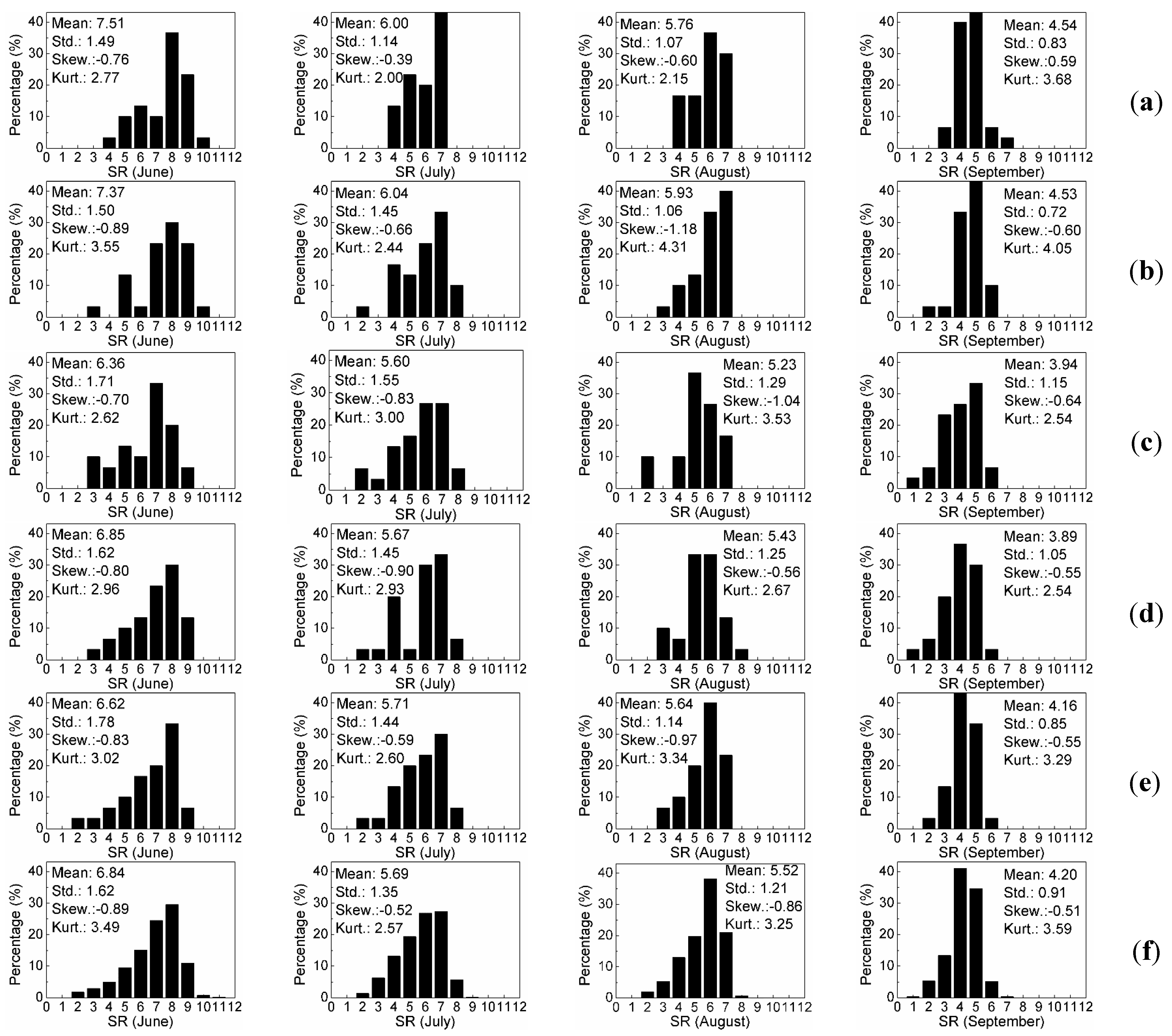
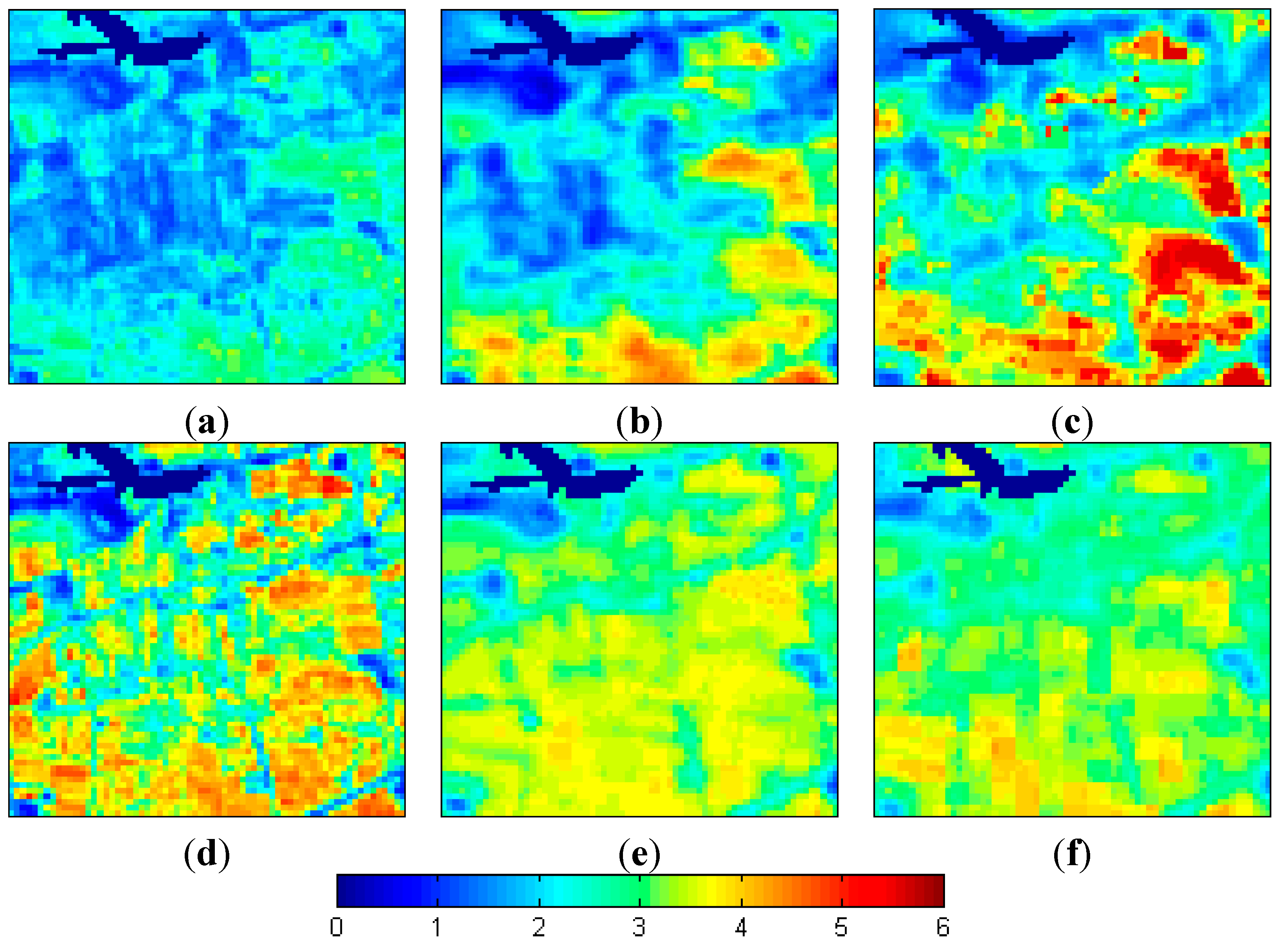
4.1. Evaluation of the ESUs Spreading in the Multi-Temporal Feature Space

The frequency distribution histograms of the 30 selected ESUs generated by different sampling strategies and the histograms of the entire site were compared from June to September (Figure 4). The ESUs selected by the random sampling method were over-sampled by 12.3% at interval 8.5–9.5 in June and by 15.9% at 6.5–7.5 in July, while these ESUs were under-sampled by 14.5% at interval 6.5–7.5 in June. The ESUs selected using the systematic sampling method were over-sampled by 12.3% at interval 8.5–9.5 in June, by 19.0% at 6.5–7.5 in August and by 15.4% at 4.5–5.5 in September but were under-sampled by 11.8% at interval 5.5–6.5 in June and by 10.0% at 2.5–3.5 in September. The ESUs selected by the land-cover-map-based method were over-sampled by 16.9% at interval 4.5–5.5 in August and by 10.0% at 2.5–3.5 in September but were under-sampled by 11.5% at interval 5.5–6.5 in August and by 11.4% at 3.5–4.5 in September. In June, the difference between the SR histogram of the ESUs selected using the SSVIP method and the histogram of the entire site was not significant. This pattern was found because the SR map in June was used as a priori knowledge for the SSVIP method. However, from July to September, the ESUs were over-sampled by 13.5% at interval 4.5–5.5 in August, but these ESUs were under-sampled by 16.0% at interval 4.5–5.5 in July. The histogram difference for the SMP approach was controlled within 5% at all the intervals from June to September, which was the lowest among the five different sampling strategies.
Four statistical indices, including the mean, standard deviation, skewness and kurtosis of the histograms, were compared in Figure 4. Compared with the entire site, the ESUs selected by the random sampling method had a larger mean by 0.67 in June, a larger skewness by 1.10 in September and a smaller kurtosis by 1.10 in August. The ESUs selected using the systematic sampling method had a larger mean by 0.53 in June and a larger kurtosis by 1.06 in August, while the land-cover-map-based method had a smaller mean by 0.48 in June and a smaller kurtosis by 1.04 in September. The SSVIP approach had similar statistical indices compared to that of the entire site in June, while this approach had a smaller mean by 0.31 in September, a smaller skewness by 0.38 in July and a smaller kurtosis by 1.05 in September. The SMP approach controlled the deviation of the mean, skewness and kurtosis from that of the entire site within 0.3, 0.2 and 0.5, respectively, which achieved the best performance among the five sampling strategies. These results suggest that sampling strategies attempting to achieve the optimal sampling in mono-temporal observations, such as the SSVIP method, may not be appropriate for long-term observing because of vegetation growth dynamics. The ESUs selected by the SMP method and the entire site had the most similar frequency distribution in the multi-temporal feature space.
Figure 4. SR frequency distribution histograms for the ESUs selected using (a) the random sampling method; (b) the systematic sampling method; (c) the land-cover map; (d) the SSVIP method and (e) the SMP method and for (f) the entire site from June to September with 30 ESUs. The horizontal axis indicates the SR within the interval [i − 0.5, i + 0.5], and the four statistical indices are mean (Mean), standard deviation (Std.), skewness (Skew.) and kurtosis (Kurt.).
Remotesensing 07 01300 g004
Figure 5 shows the average bias of the frequency distribution between the selected ESUs and the entire site in four images from June to September with different numbers of ESUs. The random sampling and systematic sampling methods had similar performance, but these two approaches were outperformed by the other three methods. The random sampling and systematic sampling methods exhibited a mean bias that exceeded 0.15 when the number of ESUs was 50. The other three methods exhibited biases of less than 0.07, 0.06 and 0.04 with 50 ESUs. The mean biases of the land-cover-map-based sampling method and the SSVIP approach exceeded that of the SMP method by at least 0.04 and 0.03, respectively. The mean bias of the SMP method was always the lowest when the number of ESUs ranged from 30 to 50, which suggests the stability of the SMP method at different numbers of ESUs.
Figure 5. Mean bias between the ESUs and the entire sites in four images generated using the random sampling, systematic sampling, sampling based on the land cover map, SSVIP and SMP methods at different number of ESUs.
Remotesensing 07 01300 g005

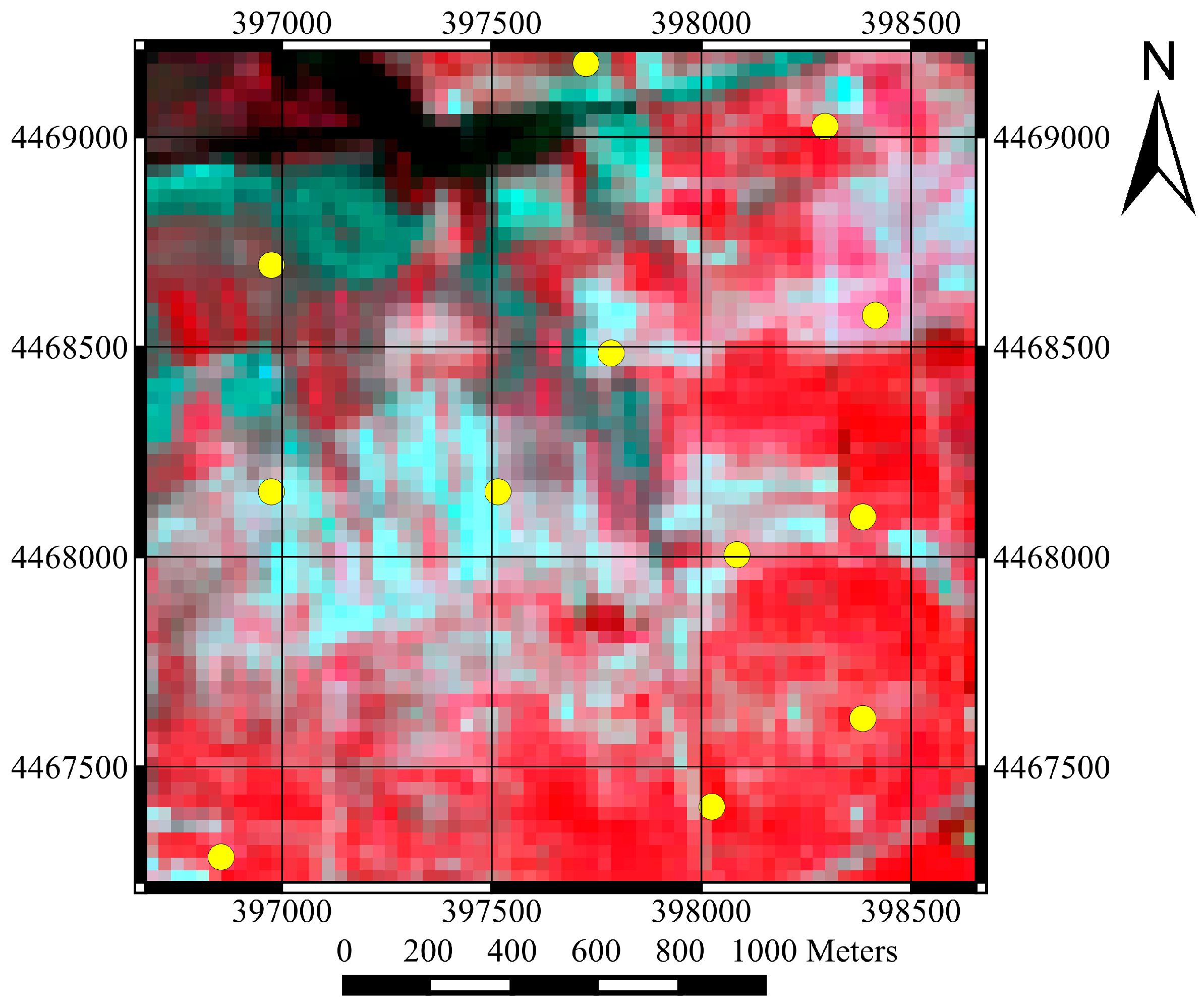
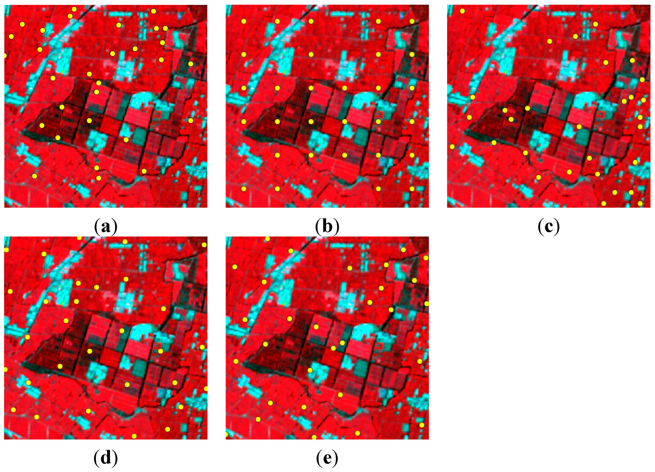
4.2. Evaluation of the ESUs Spreading in the Geographical Space

Figure 6 displays the spatial distribution of ESUs selected using the different sampling strategies. The random sampling approach produced clustering in the upper right-hand side with large blank areas over both the lower left-hand and lower right-hand portions of the image. Similar phenomena occurred for the ESUs selected using the land-cover-map-based method: the ESUs were aggregated near the right border, whereas there was only one ESU located at the upper and lower left-hand sides of the area. In contrast, the ESUs selected using the systematic sampling, SSVIP and SMP methods produced good spatial coverage of the entire area in geographical space. Figure 7 shows the NNI values for different sampling strategies with the number of ESUs varied from 30 to 50. Figure 7 indicates that the spatial distributions of the ESUs selected using random sampling and the land-cover-map-based method were similar to that of the random distribution, with the NNI values within the interval (0.9, 1.2). Systematic sampling exhibited the most dispersed spatial distribution, with the NNI value within the interval (1.6, 1.9). The SSVIP and SMP methods had NNI values within the intervals (1.5, 1.8) and (1.5, 1.7), respectively, which also indicates a dispersed distribution pattern. The results indicate that the ESUs selected using the systematic sampling, SSVIP and SMP methods were more dispersed across the area in geographical space than those generated using random sampling and the land-cover-map-based method.
Figure 6. The spatial distribution of ESUs obtained using the (a) random sampling; (b) systematic sampling; (c) land-cover map; (d) SSVIP and (e) SMP methods with 30 ESUs. ESUs located in non-vegetated areas were removed in the systematic sampling approach.
Remotesensing 07 01300 g006
Figure 7. The NNI values for the ESU pattern using the random sampling, systematic sampling, sampling based on the land-cover map, SSVIP and SMP with different numbers of ESUs.
Remotesensing 07 01300 g007

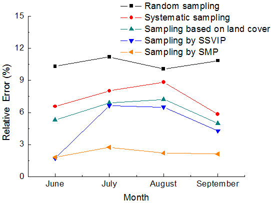
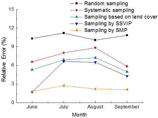
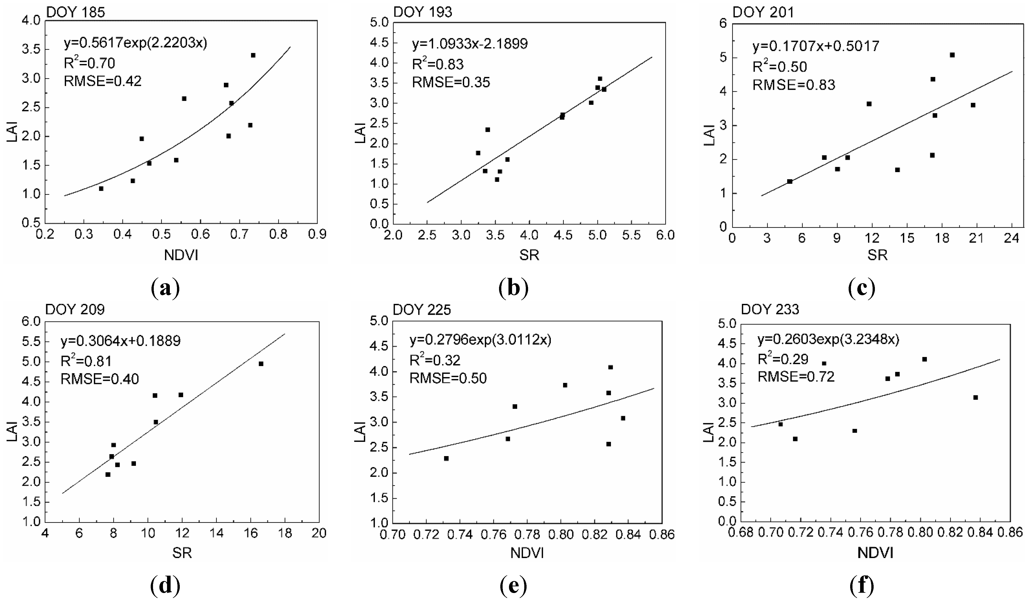
4.3. Accuracy Analysis of the LAI Reference Maps

Figure 8 shows the RMSE and the relative error (RE) between the aggregated LAI reference map and the benchmark from June to September with 30 ESUs. The LAI reference maps generated using random sampling performed the worst among the five sampling strategies, with an RMSE exceeding 0.17 and RE exceeding 10.1%. The reference map generated using the systematic sampling approach exhibited the second-worst accuracy, with the RMSE and RE exceeding 0.10 and 5.8%, respectively. The accuracy of the LAI reference map produced using the land-cover-map-based sampling method was better than the former two methods, exhibiting relatively low RMSEs of 0.08–0.15 and REs of 5.0%–7.2%. The SSVIP method had the lowest RMSE (0.05) and RE (1.7%) in June, which was similar to the performance of the SMP approach (i.e., RMSE of 0.05 and RE of 1.8%). However, the SSVIP method performed much worse than the SMP method from July to September, exhibiting RMSEs of 0.07–0.14 and REs of 4.3%–6.7%. This result was consistent with the results presented in Figure 4, which demonstrate that the difference between the SR frequency distribution of the ESUs selected using the SSVIP method and the entire site was not significant in June, while the SR frequency distributions of the ESUs were biased in some intervals from July to September. The SMP method exhibited the best performance compared with the other four methods. The RMSEs and REs were 0.04–0.06 and 1.8%–2.7%, respectively, from June to September. Compared with the land-cover-map-based method and SSVIP sampling approaches, the SMP method was able to reduce the average RMSE and RE from 0.12 and 0.10 to 0.05 and from 6.1% and 4.8% to 2.2%, respectively.
Figure 8. The (a) RMSE and (b) average relative error (RE) between the aggregated LAI reference maps generated by different sampling strategies and the reference data with 30 ESUs from June to September 2012.
Remotesensing 07 01300 g008

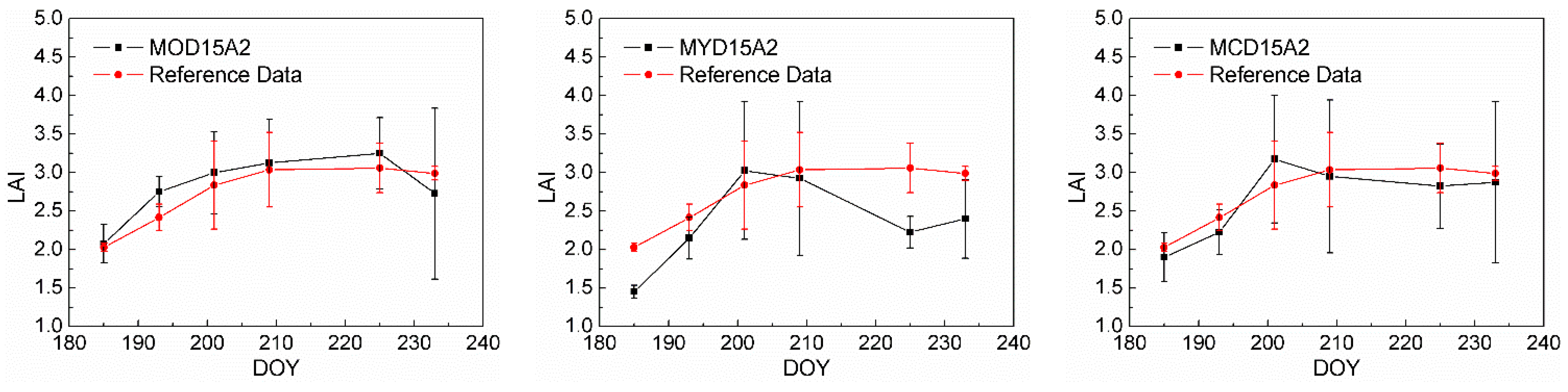
4.4. Application to LAINet Observations at Huailai Site
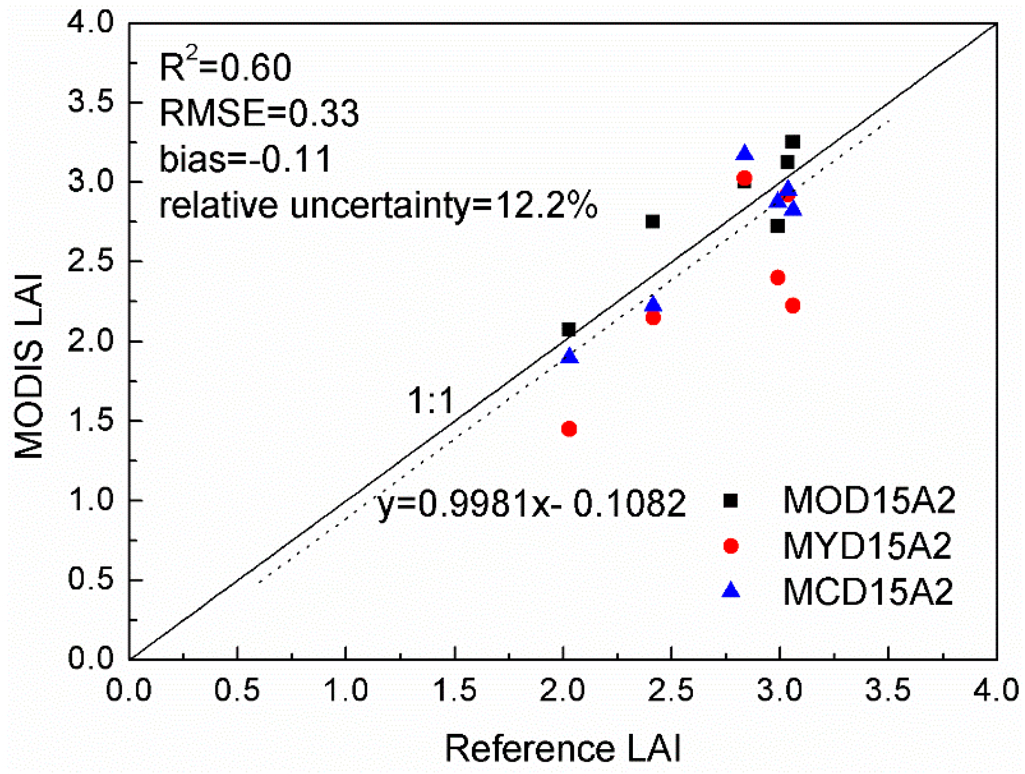
The SMP method was applied to the LAINet observations at Huailai site for the time-series validation of the MODIS C5 LAI products. Figure 9 shows the transfer functions, and the RMSEs on DOY 201 and 233 were 0.83 and 0.72. The average RMSEs on the other four days were 0.42, which was much lower than that on DOY 201 and 233. Figure 10 shows the 30-m resolution LAI reference maps at each eight-day interval, which suggests that the vegetation growth levels and the spatial heterogeneities of the area experienced significant temporal changes due to different soil, irrigation or fertilization conditions, etc.
Figure 11 shows the time-series comparison between the LAI reference maps and the corresponding MODIS LAI products at Huailai site from 4 July to 28 August. The three MODIS LAI products exhibited similar trends to those of the reference data. MOD15A2 and MCD15A2 were better correlated with the reference data than the MYD15A2 product. MODI5A2 overestimated LAI by 0.05–0.33 from DOY 193 to 225 and underestimated LAI by 0.26 on DOY 233. MCD15A2 underestimated LAI by 0.09–0.23 from DOY 185 to 193 and from DOY 209 to DOY 233 and overestimated LAI by 0.34 on DOY 201. MYD15A2 underestimated LAI by 0.58 and 0.27 from DOY 185 to 193. MYD15A2 had the lowest accuracy, with a bias that exceeded −0.59 when the crop LAI began to slightly decrease from DOY 225 to 233.
Figure 9. Transfer functions for generating the LAI reference maps at 30-m resolution on (a) DOY 185; (b) DOY 193; (c) DOY 201; (d) DOY 209; (e) DOY 225 and (f) DOY 233.
Remotesensing 07 01300 g009
Figure 10. The generated multi-temporal LAI reference maps at 30-m resolution on (a) DOY 185; (b) DOY 193; (c) DOY 201; (d) DOY 209; (e) DOY 225 and (f) DOY 233.
Remotesensing 07 01300 g010
Figure 11. Time series comparison between the mean of the LAI reference maps at Huailai site and the corresponding LAI of the three MODIS products from 4 July to 28 August 2013. The error bars represent the standard deviation of the four pixels at Huailai site from the MODIS LAI products (black) and the LAI reference maps (red).
Remotesensing 07 01300 g011
Figure 12 shows a scatter plot comparing the mean MODIS LAI values with the mean from the LAI reference maps at Huailai site from 4 July to 28 August. The relative uncertainty was defined as the ratio of the RMSE to the mean LAI. The R2, RMSE, bias and relative uncertainty were 0.60, 0.33, −0.11 and 12.2%, respectively, for the combination of the three MODIS LAI products. Table 2 shows the statistical results on the accuracy of the three products. MCD15A2 exhibited the best performance with an RMSE of 0.20, bias of −0.07 and relative uncertainty of 7.4%. MYD15A2 had the lowest accuracy.
Figure 12. Comparison between the mean MODIS LAI values and the mean of the LAI reference maps at Huailai site from 4 July to 28 August 2013.
Remotesensing 07 01300 g012
Table 2. The accuracy of the MODIS LAI products at Huailai site.
LAI ProductR2RMSEBiasRelative Uncertainty
MOD15A20.780.210.107.6%
MYD15A20.580.50−0.3618.3%
MCD15A20.820.20−0.077.4%

5. Conclusions

Focusing on the ESU assignment for the LAINet continuous observing over heterogeneous vegetated areas, a spatial sampling strategy called SMP was proposed using a combination of multi-temporal vegetation index maps and a vegetation classification map as a priori knowledge. Considering the dynamic vegetation growth processes, the SMP approach performed better than the other four sampling strategies over the vegetation cycle and was more suitable for multi-temporal LAI product validation. The PROSAIL model-based simulation analysis in the Heihe River basin demonstrated the good performance of the SMP method considering the following aspects: (1) The ESUs selected using the SMP method spread more evenly in the multi-temporal feature space and geographical space during the entire observation period. The mean bias decreased from 0.08 and 0.11 by the SSVIP method and the land-cover-map-based method, respectively, to 0.04 by the SMP method; (2) The LAI reference maps generated using the SMP method were more accurate than those generated using the other four sampling strategies over the vegetation cycle. Compared with the land-cover-map-based method and the SSVIP approaches, the average RMSE and relative error of the LAI reference maps produced with the SMP method were reduced from 0.12 and 0.10 to 0.05 and from 6.1% and 4.8% to 2.2%, respectively. The performance of the SMP method was robust to variations in the number of ESUs and to different time intervals. These improvements generate more accurate LAI reference maps and promise more accurate long-term validation over heterogeneous vegetated areas for moderate- and coarse-resolution LAI products.
The SMP approach was applied to determine the locations of observation nodes for the LAINet at the Huailai Remote Sensing Experimental Station in Beijing, China, from 4 July to 28 August 2013. Multi-temporal LAI reference maps were generated to validate three MODIS C5 LAI products. The validation results suggested that the R2, RMSE, bias and relative uncertainty were 0.60, 0.33, −0.11 and 12.2%, respectively, for the combination of the three MODIS LAI products. Among the three products, MCD15A2 exhibited the best performance with an RMSE of 0.20, bias of −0.07 and relative uncertainty of 7.4%. MYD15A2 exhibited the lowest accuracy. Future efforts are needed to obtain more long-term validation datasets using the SMP approach on different vegetation types for validating moderate-resolution LAI products in time series.

Acknowledgments

This research was supported by the National Natural Science Foundation of China (No. 41271366), the National Basic Research Program of China (No. 2013CB733401) and the National High Technology Research and Development Program of China (No. 2012AA12A305; No. 2012AA12A304). The authors thank the HiWATER project for providing the field measurement dataset.

Author Contributions

Jing Li and Qinhuo Liu designed the research. Yonghua Qu collected and provided the dataset of LAINet observations. Yelu Zeng and Baodong Xu analyzed the data and wrote the paper. Gaofei Yin and Jing Zhao interpreted the results. Alfredo R. Huete aided with the discussion and the manuscript revision.

Conflicts of Interest

The authors declare no conflict of interest.

References

  1. Chen, J.M.; Black, T. Defining leaf area index for non-flat leaves. Plant Cell Environ. 1992, 15, 421–429. [Google Scholar] [CrossRef]
  2. Stenberg, P. Correcting LAI-2000 estimates for the clumping of needles in shoots of conifers. Agric. For. Meteorol. 1996, 79, 1–8. [Google Scholar] [CrossRef]
  3. Bonan, G.B. Land-atmosphere interactions for climate system models: Coupling biophysical, biogeochemical, and ecosystem dynamical processes. Remote Sens. Environ. 1995, 51, 57–73. [Google Scholar] [CrossRef]
  4. Knyazikhin, Y.; Martonchik, J.; Myneni, R.; Diner, D.; Running, S. Synergistic algorithm for estimating vegetation canopy leaf area index and fraction of absorbed photosynthetically active radiation from MODIS and MISR data. J. Geophys. Res. Atmos. 1998, 103, 32257–32275. [Google Scholar] [CrossRef]
  5. Bacour, C.; Baret, F.; Beal, D.; Weiss, M.; Pavageau, K. Neural network estimation of LAI, FAPAR, FCOVER and LAIXCAB, from top of canopy MERIS reflectance data: Principles and validation. Remote Sens. Environ. 2006, 105, 313–325. [Google Scholar] [CrossRef]
  6. Zhang, X.; Friedl, M.A.; Schaaf, C.B. Global vegetation phenology from Moderate Resolution Imaging Spectroradiometer (MODIS): Evaluation of global patterns and comparison with in situ measurements. J. Geophys. Res. Biogeosci. 2006, 111, G04017. [Google Scholar]
  7. Baret, F.; Hagolle, O.; Geiger, B.; Bicheron, P.; Miras, B.; Huc, M.; Berthelot, B.; Niño, F.; Weiss, M.; Samain, O.; et al. LAI, FAPAR and FCOVER cyclopes global products derived from vegetation: Part 1: Principles of the algorithm. Remote Sens. Environ. 2007, 110, 275–286. [Google Scholar]
  8. Ganguly, S.; Samanta, A.; Schull, M.A.; Shabanov, N.V.; Milesi, C.; Nemani, R.R.; Knyazikhin, Y.; Myneni, R.B. Generating vegetation leaf area index earth system data record from multiple sensors. Part 2: Implementation, analysis and validation. Remote Sens. Environ. 2008, 112, 4318–4332. [Google Scholar]
  9. Ganguly, S.; Schull, M.A.; Samanta, A.; Shabanov, N.V.; Milesi, C.; Nemani, R.R.; Knyazikhin, Y.; Myneni, R.B. Generating vegetation leaf area index earth system data record from multiple sensors. Part 1: Theory. Remote Sens. Environ. 2008, 112, 4333–4343. [Google Scholar] [CrossRef]
  10. Chen, J.M.; Pavlic, G.; Brown, L.; Cihlar, J.; Leblanc, S.; White, H.; Hall, R.; Peddle, D.; King, D.; Trofymow, J.; et al. Derivation and validation of Canada-wide coarse-resolution leaf area index maps using high-resolution satellite imagery and ground measurements. Remote Sens. Environ. 2002, 80, 165–184. [Google Scholar]
  11. Li, X.; Cheng, G.; Liu, S.; Xiao, Q.; Ma, M.; Jin, R.; Che, T.; Liu, Q.; Wang, W.; Qi, Y. Heihe watershed allied telemetry experimental research (Hiwater): Scientific objectives and experimental design. Bull. Am. Meteorol. Soc. 2013, 94, 1145–1160. [Google Scholar] [CrossRef]
  12. Li, X.; Li, X.; Li, Z.; Ma, M.; Wang, J.; Xiao, Q.; Liu, Q.; Che, T.; Chen, E.; Yan, G. Watershed allied telemetry experimental research. J. Geophys. Res. Atmos. 2009, 114. [Google Scholar] [CrossRef]
  13. Tian, Y.; Woodcock, C.E.; Wang, Y.; Privette, J.L.; Shabanov, N.V.; Zhou, L.; Zhang, Y.; Buermann, W.; Dong, J.; Veikkanen, B.; et al. Multiscale analysis and validation of the MODIS LAI product: Ii. Sampling strategy. Remote Sens. Environ. 2002, 83, 431–441. [Google Scholar]
  14. Morisette, J.T.; Baret, F.; Privette, J.L.; Myneni, R.B.; Nickeson, J.E.; Garrigues, S.; Shabanov, N.V.; Weiss, M.; Fernandes, R.A.; Leblanc, S.G.; et al. Validation of global moderate-resolution LAI products: A framework proposed within the CEOS land product validation subgroup. IEEE Trans. Geosci. Remote Sens. 2006, 44, 1804–1817. [Google Scholar]
  15. Zeng, Y.L.; Li, J.; Liu, Q.H. Global LAI ground validation dataset and product validation framework: A review. Adv. Earth Sci. 2012, 27, 165–174. [Google Scholar]
  16. Whitford, K.; Colquhoun, I.; Lang, A.; Harper, B. Measuring leaf area index in a sparse eucalypt forest: A comparison of estimates from direct measurement, hemispherical photography, sunlight transmittance and Allometric regression. Agric. For. Meteorol. 1995, 74, 237–249. [Google Scholar] [CrossRef]
  17. Nackaerts, K.; Coppin, P.; Muys, B.; Hermy, M. Sampling methodology for LAI measurements with LAI-2000 in small forest stands. Agric. For. Meteorol. 2000, 101, 247–250. [Google Scholar] [CrossRef]
  18. Law, B.; Van Tuyl, S.; Cescatti, A.; Baldocchi, D. Estimation of leaf area index in open-canopy ponderosa pine forests at different successional stages and management regimes in Oregon. Agric. For. Meteorol. 2001, 108, 1–14. [Google Scholar] [CrossRef]
  19. Buermann, W.; Helmlinger, M. Safari 2000 LAI and FPAR Measurements at SUA Pan, Botswana, Dry Season 2000. Available online: http://daac.ornl.gov//S2K/safari.shtml (accessed on 26 December 2004).
  20. Majasalmi, T.; Rautiainen, M.; Stenberg, P.; Rita, H. Optimizing the sampling scheme for LAI-2000 measurements in a boreal forest. Agric. For. Meteorol. 2012, 154, 38–43. [Google Scholar] [CrossRef]
  21. Minasny, B.; McBratney, A.B. A conditioned Latin hypercube method for sampling in the presence of ancillary information. Comput. Geosci. 2006, 32, 1378–1388. [Google Scholar] [CrossRef]
  22. Mulder, V.; de Bruin, S.; Schaepman, M. Representing major soil variability at regional scale by constrained Latin hypercube sampling of remote sensing data. Int. J. Appl. Earth Obs. Geoinf. 2013, 21, 301–310. [Google Scholar] [CrossRef]
  23. Yang, L.; Zhu, A.X.; Qi, F.; Qin, C.Z.; Li, B.; Pei, T. An integrative hierarchical stepwise sampling strategy for spatial sampling and its application in digital soil mapping. Int. J. Geogr. Inf. Sci. 2013, 27, 1–23. [Google Scholar] [CrossRef]
  24. Zeng, Y.L.; Li, J.; Liu, Q.H.; Li, L.H.; Xu, B.D.; Yin, G.F.; Peng, J.J. A sampling strategy for remotely sensed LAI product validation over heterogeneous land surface. IEEE J. Sel. Top. Appl. Earth Obs. Remote Sens. 2014, 7, 3128–3142. [Google Scholar] [CrossRef]
  25. Baret, F.; Weiss, M.; Allard, D.; Garrigues, S.; Leroy, M.; Jeanjean, H.; Fernandes, R.; Myneni, R.; Privette, J.; Morisette, J.; et al. Valeri: A Network of Sites and a Methodology for the Validation of Medium Spatial Resolution Land Satellite Products. Available online: http://w3.avignon.inra.fr/valeri/ (accessed on 28 December 2005).
  26. Martinez, B.; García-Haro, F.; Camacho-de Coca, F. Derivation of high-resolution leaf area index maps in support of validation activities: Application to the cropland Barrax site. Agric. For. Meteorol. 2009, 149, 130–145. [Google Scholar] [CrossRef]
  27. Wang, Y.; Woodcock, C.E.; Buermann, W.; Stenberg, P.; Voipio, P.; Smolander, H.; Häme, T.; Tian, Y.; Hu, J.; Knyazikhin, Y. Evaluation of the MODIS LAI algorithm at a coniferous forest site in Finland. Remote Sens. Environ. 2004, 91, 114–127. [Google Scholar] [CrossRef]
  28. Claverie, M.; Vermote, E.F.; Weiss, M.; Baret, F.; Hagolle, O.; Demarez, V. Validation of coarse spatial resolution LAI and FAPAR time series over cropland in southwest France. Remote Sens. Environ. 2013, 139, 216–230. [Google Scholar] [CrossRef]
  29. Heiskanen, J.; Rautiainen, M.; Stenberg, P.; Mõttus, M.; Vesanto, V.H.; Korhonen, L.; Majasalmi, T. Seasonal variation in MODIS LAI for a boreal forest area in Finland. Remote Sens. Environ. 2012, 126, 104–115. [Google Scholar] [CrossRef]
  30. Ryu, Y.; Verfaillie, J.; Macfarlane, C.; Kobayashi, H.; Sonnentag, O.; Vargas, R.; Ma, S.; Baldocchi, D.D. Continuous observation of tree leaf area index at ecosystem scale using upward-pointing digital cameras. Remote Sens. Environ. 2012, 126, 116–125. [Google Scholar] [CrossRef]
  31. Qu, Y.; Han, W.; Fu, L.; Li, C.; Song, J.; Zhou, H.; Bo, Y.; Wang, J. Lainet—A wireless sensor network for coniferous forest leaf area index measurement: Design, algorithm and validation. Comput. Electron. Agric. 2014, 108, 200–208. [Google Scholar] [CrossRef]
  32. Qu, Y.; Zhu, Y.; Han, W.; Wang, J.; Ma, M. Crop leaf area index observations with a wireless sensor network and its potential for validating remote sensing products. IEEE J. Sel. Top. Appl. Earth Obs. Remote Sens. 2014, 7, 431–444. [Google Scholar] [CrossRef]
  33. Wang, N.; Zhang, N.; Wang, M. Wireless sensors in agriculture and food industry—Recent development and future perspective. Comput. Electron. Agric. 2006, 50, 1–14. [Google Scholar] [CrossRef]
  34. Selavo, L.; Wood, A.; Cao, Q.; Sookoor, T.; Liu, H.; Srinivasan, A.; Wu, Y.; Kang, W.; Stankovic, J.; Young, D. Luster: Wireless sensor network for environmental research. In Proceedings of the 5th International Conference on Embedded Networked Sensor Systems, Sydney, Australia, 4–9 November 2007; pp. 103–116.
  35. Jin, R.; Li, X.; Yan, B.; Li, X.; Luo, W.; Ma, M.; Guo, J.; Kang, J.; Zhu, Z.; Zhao, S. A nested eco-hydrological wireless sensor network for capturing the surface heterogeneity in the midstream area of the Heihe River Basin, China. IEEE Geosci. Remote Sens. Lett. 2014, 11, 2015–2019. [Google Scholar] [CrossRef]
  36. Hengl, T.; Rossiter, D.G.; Stein, A. Soil sampling strategies for spatial prediction by correlation with auxiliary maps. Soil Res. 2003, 41, 1403–1422. [Google Scholar] [CrossRef]
  37. Clark, P.J.; Evans, F.C. Distance to nearest neighbor as a measure of spatial relationships in populations. Ecology 1954, 35, 445–453. [Google Scholar] [CrossRef]
  38. Kim, J.; Guo, Q.; Baldocchi, D.; Leclerc, M.; Xu, L.; Schmid, H. Upscaling fluxes from tower to landscape: Overlaying flux footprints on high-resolution (Ikonos) images of vegetation cover. Agric. For. Meteorol. 2006, 136, 132–146. [Google Scholar] [CrossRef]
  39. Chen, B.; Coops, N.C.; Fu, D.; Margolis, H.A.; Amiro, B.D.; Black, T.A.; Arain, M.A.; Barr, A.G.; Bourque, C.P.A.; Flanagan, L.B. Characterizing spatial representativeness of flux tower eddy-covariance measurements across the Canadian carbon program network using remote sensing and footprint analysis. Remote Sens. Environ. 2012, 124, 742–755. [Google Scholar] [CrossRef]
  40. Vermote, E.F.; Tanré, D.; Deuze, J.L.; Herman, M.; Morcette, J.J. Second simulation of the satellite signal in the solar spectrum, 6s: An overview. IEEE Trans. Geosci. Remote Sens. 1997, 35, 675–686. [Google Scholar] [CrossRef]
  41. Jacquemoud, S.; Verhoef, W.; Baret, F.; Bacour, C.; Zarco-Tejada, P.J.; Asner, G.P.; François, C.; Ustin, S.L. Prospect + sail models: A review of use for vegetation characterization. Remote Sens. Environ. 2009, 113, S56–S66. [Google Scholar] [CrossRef]
  42. Vermote, E. Product Accuracy/Uncertainty: Mod09, Surface Reflectance; Atmospheric Correction Algorithm Product. In: MODIS Data Products Catalog (Eos Am Platform). Available online: http://modarch.gsfc.nasa.gov/MODIS/RESULTS/DATAPROD/ (accessed on 27 December 2000).
  43. Chen, J.M. Optically-based methods for measuring seasonal variation of leaf area index in boreal conifer stands. Agric. For. Meteorol. 1996, 80, 135–163. [Google Scholar] [CrossRef]
  44. Tan, B.; Woodcock, C.; Hu, J.; Zhang, P.; Ozdogan, M.; Huang, D.; Yang, W.; Knyazikhin, Y.; Myneni, R. The impact of gridding artifacts on the local spatial properties of MODIS data: Implications for validation, compositing, and band-to-band registration across resolutions. Remote Sens. Environ. 2006, 105, 98–114. [Google Scholar] [CrossRef]
  45. Weiss, M.; Baret, F.; Garrigues, S.; Lacaze, R. LAI and FAPAR cyclopes global products derived from vegetation. Part 2: Validation and comparison with MODIS collection 4 products. Remote Sens. Environ. 2007, 110, 317–331. [Google Scholar]
  46. Yang, W.; Shabanov, N.; Huang, D.; Wang, W.; Dickinson, R.; Nemani, R.; Knyazikhin, Y.; Myneni, R. Analysis of leaf area index products from combination of MODIS terra and aqua data. Remote Sens. Environ. 2006, 104, 297–312. [Google Scholar] [CrossRef]

