
Transformer in UAV Image-Based Weed Mapping


1
Department of Agricultural Technology, Norwegian Institute of Bioeconomy Research (NIBIO), P.O. Box 115, NO-1431 Ås, Norway
2
Department of Invertebrate Pests and Weeds in Forestry, Agriculture and Horticulture, Norwegian Institute of Bioeconomy Research (NIBIO), P.O. Box 115, NO-1431 Ås, Norway
*
Author to whom correspondence should be addressed.
Remote Sens. 2023, 15(21), 5165; https://doi.org/10.3390/rs15215165
Submission received: 26 August 2023
/
Revised: 6 October 2023
/
Accepted: 26 October 2023
/
Published: 29 October 2023
(This article belongs to the Special Issue Advanced Application of Artificial Intelligence and Machine Vision in Remote Sensing II)
Abstract
:Weeds affect crop yield and quality due to competition for resources. In order to reduce the risk of yield losses due to weeds, herbicides or non-chemical measures are applied. Weeds, especially creeping perennial species, are generally distributed in patches within arable fields. Hence, instead of applying control measures uniformly, precision weeding or site-specific weed management (SSWM) is highly recommended. Unmanned aerial vehicle (UAV) imaging is known for wide area coverage and flexible operation frequency, making it a potential solution to generate weed maps at a reasonable cost. Efficient weed mapping algorithms need to be developed together with UAV imagery to facilitate SSWM. Different machine learning (ML) approaches have been developed for image-based weed mapping, either classical ML models or the more up-to-date deep learning (DL) models taking full advantage of parallel computation on a GPU (graphics processing unit). Attention-based transformer DL models, which have seen a recent boom, are expected to overtake classical convolutional neural network (CNN) DL models. This inspired us to develop a transformer DL model for segmenting weeds, cereal crops, and ‘other’ in low-resolution RGB UAV imagery (about 33 mm ground sampling distance, g.s.d.) captured after the cereal crop had turned yellow. Images were acquired during three years in 15 fields with three cereal species (Triticum aestivum, Hordeum vulgare, and Avena sativa) and various weed flora dominated by creeping perennials (mainly Cirsium arvense and Elymus repens). The performance of our transformer model, 1Dtransformer, was evaluated through comparison with a classical DL model, 1DCNN, and two classical ML methods, i.e., random forest (RF) and k-nearest neighbor (KNN). The transformer model showed the best performance with an overall accuracy of 98.694% on pixels set aside for validation. It also agreed best and relatively well with ground reference data on total weed coverage, R2 = 0.598. In this study, we showed the outstanding performance and robustness of a 1Dtransformer model for weed mapping based on UAV imagery for the first time. The model can be used to obtain weed maps in cereals fields known to be infested by perennial weeds. These maps can be used as basis for the generation of prescription maps for SSWM, either pre-harvest, post-harvest, or in the next crop, by applying herbicides or non-chemical measures.
1. Introduction
Weeds may reduce crop yield because they compete with crops for available resources including water, nutrients, and light. Weeds, especially creeping perennial species propagating through clonal growth, are often patchily distributed in arable fields [1,2,3]. Hence, the normal practice of broadcast (uniform) weed control may cause unnecessary herbicide use and increase chemical residues in the harvested product and the weeds’ resistance to herbicide. Site-specific weed management (SSWM) considers the weeds’ spatial distribution and within-field variation, targeting weed control precisely to weed pressure and even weed species [4]. SSWM can potentially reduce costs and use of herbicides, fossil fuels, and energy when herbicide is applied only in regions where weeds are located [5,6,7,8,9,10,11,12].
The implementation of SSWM relies on accurate weed monitoring [13,14,15]. Human monitoring is time-consuming, expensive, and not suitable for large-scale field applications [16,17]. Unmanned aerial vehicle (UAV)-based monitoring offers high flexibility in terms of temporal, spectral, and spatial resolutions. Different imaging sensors like visible, multispectral, hyperspectral, and thermal ones make UAVs capable of capturing more complete information of the fields and facilitate precision weed management [18]. Compared with ground-based vehicles, UAVs cover larger areas in a shorter time without being impeded by adverse field conditions [19]. Such flexibility makes UAVs attractive platforms for weed mapping [20]. UAV imagery must be processed with segmentation algorithms for effective weed mapping. Segmentation methods can be divided into two major categories, index-based and learning-based. Many vegetation indices (Vis) generated from images, depending on their different spectral resolution and spectral ranges, can be used for weed mapping. Traditional threshold-based image segmentation was often implemented in either Lab or HSV color spaces [21]. Vis calculated for UAV RGB imagery acquired pre-harvest in winter wheat often did not correlate well with visually scored weed pressure of annual/biannual weed species [22]. Rasmussen et al. (2019) used the normalized excess green index to map the perennial creeping thistle (Cirsium arvense) in late-season cereals based on low-altitude UAV imagery (corresponding to 3–17 mm ground sample distance, g.s.d.) [23]. High accuracies were achieved, but manual thresholding was needed, as also reported by Hamouz et al., (2009) who explored VI-based mapping of Cirsium arvense in ripe wheat based on multispectral (red, green, near infrared) low-resolution imagery (100 mm g.s.d.) [24]. Index-based approaches were not considered in this study as the threshold varies from image to image and thus lack robustness and generalizability.
The learning-based methods can better cope with the challenges which index-based models are facing, and are generally preferred in practice [25]. Learning-based models can be further divided into classical machine learning (ML) and deep learning (DL) models depending on whether they are able to perform automatic feature extraction [26]. Classical ML has been widely used for weed mapping by classifying pixels of weeds and crops in proximal (near-ground) imagery (e.g., Ahmed et al., (2012)) [27] and aerial imagery. For example, Su et al. (2022) mapped the annual grass weed blackgrass (Alopecurus myosuroides) using UAV multispectral (MS) imagery and a random forest (RF) classifier in mid-season wheat (Triticum aestivum) [28]. Gašparović et al. (2020) utilized a fusion of RF-based supervised and K-means clustering-based unsupervised classification methods to map creeping thistle (Cirsium arvense) and Roman chamomile (Chamaemelum nobile), also a perennial weed, in ripe winter oat (Avena sativa) using UAV RGB imagery [29].
Even though traditional ML models have reached good performances in weed mapping applications, DL is generally more favorable because of its capability in task-driven model optimization through automatic feature extraction which updates the weights of layer(s) inside the model based on how well it performs [30,31,32]. DL is also able to extract more representative information directly from raw data, and thus has dramatically outperformed traditional ML counterparts in many cases [28,33]. DL models, both classical CNN-based and the latest transformer-based ones, have promoted weed mapping due to their flexibilities in managing input data in different dimensionalities.
Classical DL models refers mostly to convolutional neural network (CNN) models and have been the state-of-the-art models for different tasks for a time. The plain fully connected network (FCN) has demonstrated its great capacity in plant segmentation; more sophisticated network architectures considering the different levels of information contained in deeper and shallower layers of CNNs have even further improved these models’ performances [34]. For SSWM purposes, most DL models take 2D images as input to either classify or detect weeds at the early growth stages based on high-resolution RGB imagery [35]. For example, Huang et al. (2018) separated weed and rice in UAV RGB imagery using a CNN-based DL model, and found a better performance compared to a classical ML model, the support vector machines (SVM) [36]. Fawakherji et al. (2019) used a Unet to separate weeds from crop (sunflower, carrot, and sugar beet) using RGB imagery captured by a ground-based robot [37]. Milioto et al. (2018) applied a simple 2D CNN model to accurately segment sugar beet and weed in real time based on the combination of both RGB imagery and different indices derived from them [38]. SegNet, another 2D CNN model, was applied to segment weed, carrot and soil using RGB imagery in high accuracy [39]. For later growth stages, Fraccaro et al. (2022) used DL models (UNET-ResNet) to detect the annual blackgrass (Alopecurus myosuroides) in winter wheat based on UAV RGB and MS imagery at the time when the flowering heads of the weed were above the crop, with, however, low accuracy [40].
Transformer models, which have had extraordinary success in language translation first and then in image classification and semantic segmentation [41,42,43], are expected to outperform and even replace CNN-based DL models, especially when the data sample is large enough. Additionally, semantic segmentation is known for its demand for a large and accurately labeled dataset [44,45], which makes the data preparation process much more labor-intensive as all pixels of at least one class inside the image must be annotated. The annotation itself is time consuming and even more prone to errors when the weeds, the surrounding crop, and the soil are mixed in low-resolution UAV imagery.
A transformer is a purely attention-based model, which was inspired by the human perception process of focusing on parts of the information each time. A transformer aggregates global information from the complete set of input features with low computation cost, while CNN-based models generally have a restricted receptive field defined by the small kernel size. Multi-Head Attention was adopted to further increase the flexibility of the information to be focused and potentially to boost the performance of a transformer model [46]. Transformer models have recently also proved to perform better than CNN-based DL models in different weeds and crop classifications [47,48], and even in semantical segmentation of different weeds species [48]. However, these studies focused on high-resolution imagery taken by proximal sensors or UAVs flying at low altitudes, and DL-based semantic segmentation frameworks were only implemented in a 2D space, e.g., both 2D transformer and 2D CNN. Studies on remotely sensed data at much lower spatial resolutions for transformer models capable of mapping weeds in arable fields have, to our knowledge, not been addressed before but are necessary to exploit the possibilities of off-the-shelf UAVs and imaging systems in practice, capturing imagery at the maximum allowed flight altitude, thus at lower spatial resolution.
With the upcoming need of applying SSWM in Norwegian cereal production, we designed and evaluated a transformer DL model to map creeping perennial weeds in small-grain cereal fields at the crops’ late-season ripening growth stages. The model was based on the RGB color information in low-resolution UAV imagery. Late-season mapping should be sound for perennial weeds in small-grain cereals. At this time, the creeping perennials have fully emerged, are still mainly green while the crop is yellow, and their spatial distribution will not change significantly between the mapping and the weeding operation. The subgoals were to design the following models: (1) an effective one-dimensional transformer model, 1Dtransformer, with skip concatenation to classify pixels of weeds, crop and ‘other’ classes, (2) a CNN-based one-dimensional DL model, 1DCNN, to highlight the differences between attention- and CNN-based models, and (3) two classical ML models to compare the performances of DL and ML models. Ablation studies on 1Dtransformer were conducted to compare the contribution of skip concatenation in the architecture. All model outputs were validated against ground reference data on total weed coverage visually scored in sub-field plots.
2. Materials and Methods
2.1. Study Site and Ground Reference Data
Cereals play an important role in Norwegian agricultural production [49]. Grain quality is often affected due to infestations by creeping perennial weeds, an effect that may be reduced by SSWM strategies. UAV imagery and ground reference data were collected in 15 cereal fields, including spring and winter wheat (Triticum aestivum), barley (Hordeum vulgare), and oat (Avena sativa). The fields were infested with various weed species compositions and data were collected for three years (2020–2022) in early autumn (August) when the cereals had already turned yellow (Table 1). All fields were commercial conventional fields in Norway, either in the Follo region, east of fiord Oslofjorden, or in the Innlandet region, south and east of lake Mjøsa. All fields were sown with crop row distances of about 0.125 m, the common practice in Northern Europe.
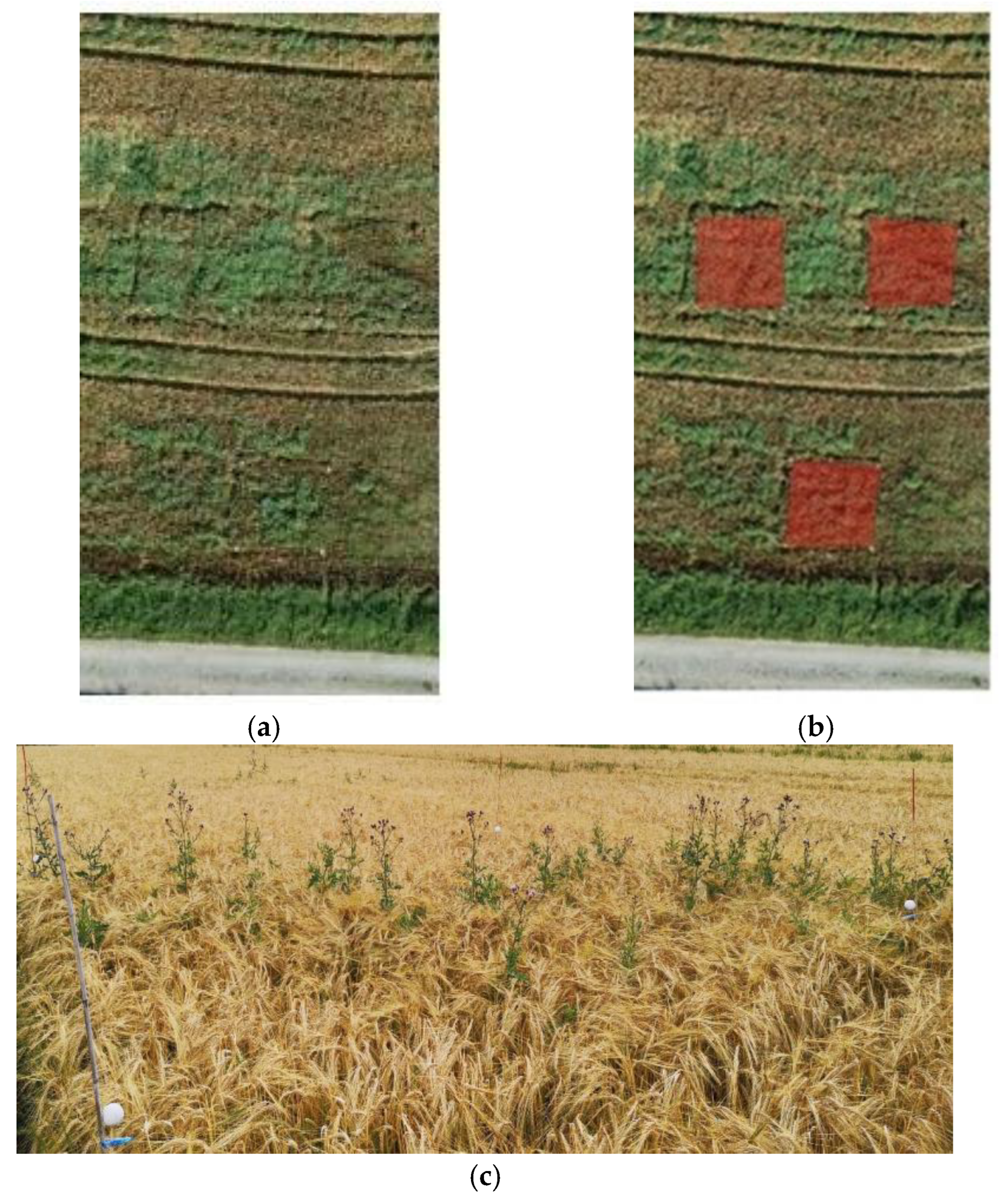
Ground reference data on coverage of weeds, crop and soil was registered by persons with various experience through in-field inspection in square plots (16 m2) (Figure 1). Data were estimated via human vision, and total weed coverage, i.e., the percentage of a plot’s area covered by weeds when projecting the weed plants vertically to ground level, was assigned to each plot. Weed coverage values could be in the range of 0–100%. Plots were located semi-randomly in each field to constitute a range in weediness from near zero to heavy perennial weed infestation. Plot corners were geo-referenced via precise hand-held GNSS (GeoXH GeoExplorer 6000 series, Trimble, Westminster, CO, USA) to be extracted from processed UAV orthomosaics and used to validate the models’ performances in weed coverage estimation. Plot corners were temporarily marked by white styrofoam balls just above the crop stand. In total, 134 plots were assessed.
2.2. UAV Imaging and Preprocessing
UAV imagery was acquired with a P4RTK off-the-shelf drone (SZ DJI Technology Co., Ltd., Shenzhen, China) in nadir (down-looking) mode at a flight altitude of 120 m above ground level (a.g.l.). Although this flight altitude results in a relatively low spatial resolution of around 33 mm ground sample distance (g.s.d.), it was chosen as it is the maximum allowed in the European Union and Norway, and in consequence, considered as most applicable for practical drone missions due to the maximization of area covered per flight. Imagery was collected at field scale at a time close to the ground reference data (0 ± 5 days) (Table 1). During data acquisition, the cloud cover varied from clear to overcast skies, resulting in a wide range of illumination conditions. In total, 15 fields were overflown for three years, from 2020–2022. Imagery was processed to georeferenced orthomosaics with the commercial photogrammetric processing software Metashape (v. 1.8.4) (Agisoft LLC, St. Petersburg, Russia) using default RGB image processing settings and lens corrections as provided by the manufacturer. Exterior orientation was established through the on-board inertial measurement system. A slight spatial misalignment of ground reference plots and orthomosaics was corrected by manual alignment of the vector geometries of the registration plots with the white Styrofoam plot markers visible in the orthomosaics.
2.3. Pixel Annotation for Model Development
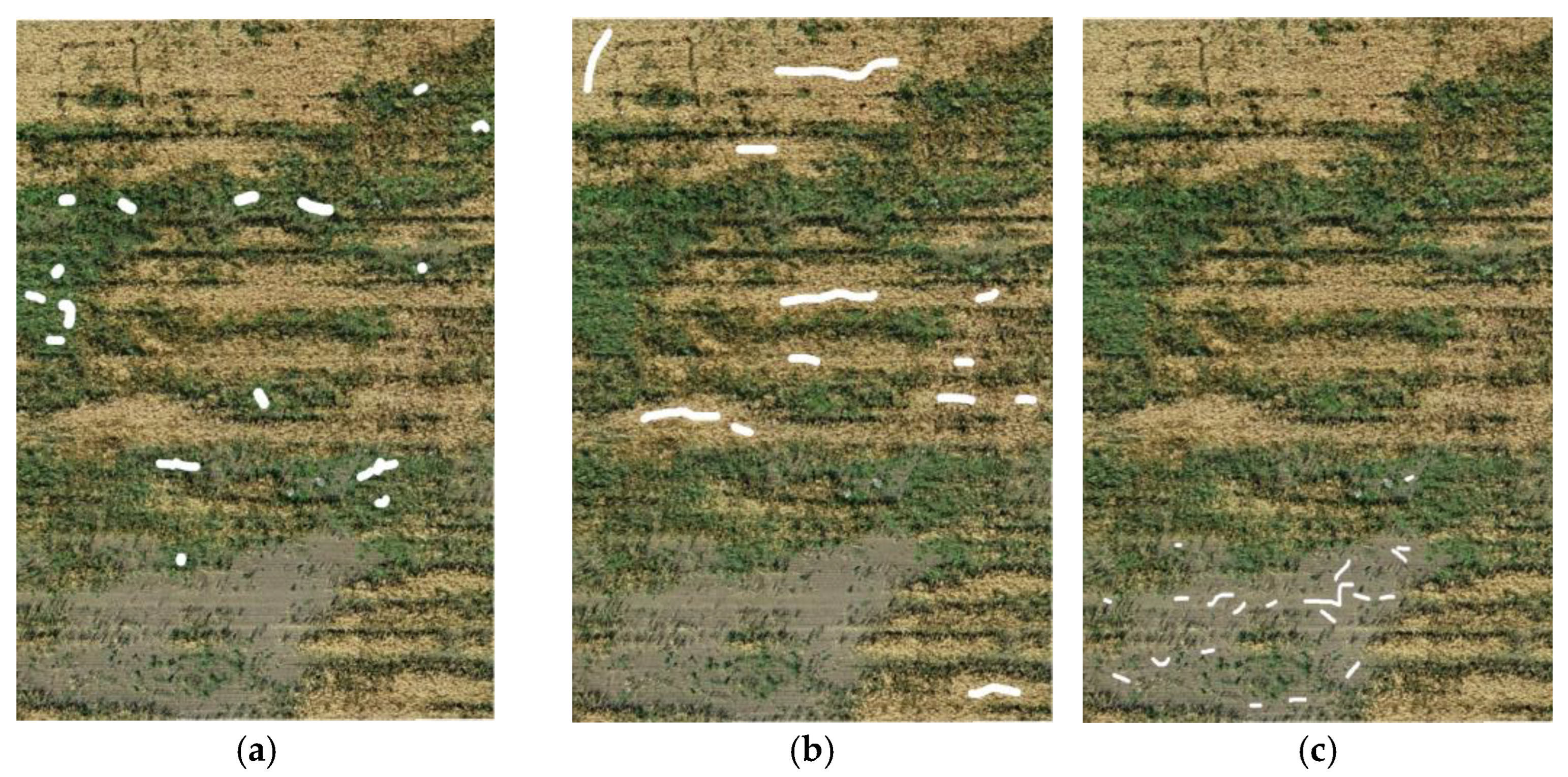
Images were annotated in GIMP 2.6 (GNU Image Manipulation Program) software by selecting sample pixels of interests manually. A total of 0.044 million, 0.329 million, and 0.392 million pixels were annotated representing the three classes of weeds, crops, and other (mainly bare soil, but also roads, buildings, and shadows), respectively (Figure 2). The collected pixels were further used for the classification models’ calibration and evaluated via 5-fold cross-validation. Pixels that fell into plots for ground reference were excluded carefully in the sample data set for model development in order to test classification performance in a later stage with a completely unseen data set to lower the chance of overfitting and make the model more robust for application.
2.4. Classification Models
2.4.1. Transformer
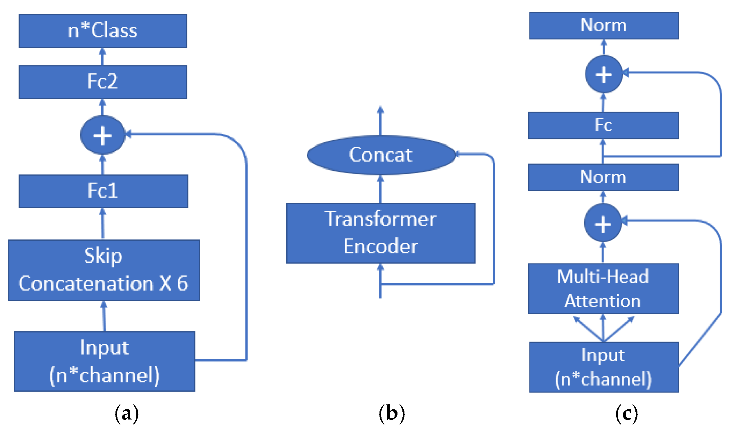
The core component of a transformer is the transformer encoder in which attention is placed. Since only 1D color information of each pixel was targeted, a 1DTransformer was specifically adapted to manage the classification task. Fully connected (Fc) layers were used to map the matrices between different dimensions. Besides a commonly used residual structure inside each transformer encoder, skip concatenation was also implemented to make full use of the lower-level features to promote model performance in pixel classification (Figure 3).
2.4.2. CNN
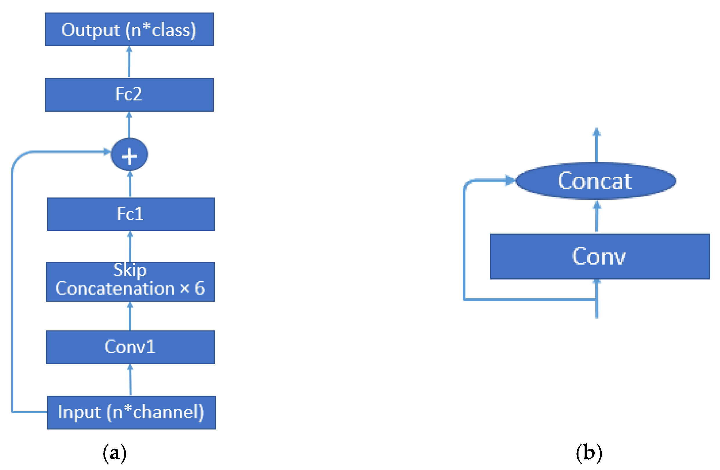
The DenseNet-like 1DCNN architecture with one convolution layer, six skip concatenation blocks, and two fully connected layers was designed to perform pixel classifications using a CNN (Figure 4). Skip concatenation was also implemented in this CNN in order to increase the presence of lower-level features.
2.4.3. RF and KNN
Two classical ML algorithms, RF [50] and KNN [51], which have been extensively used in different classification tasks, were included for comparisons [52,53]. The implementation of both RF and k-NN was in the scikit-learn package [54]. Default values of trees = 100 and max_features = 2 were selected for RF, but the max_depth was tuned from 5 to 100 in increments of 5; the optimal tree depth was chosen when the model reached the highest average validation accuracy in stratified 5-fold cross-validation. For k-NN, Euclidean distance was chosen and the number of neighbors, k, was tuned from 5 to 100 in increments of 5; the k was selected when the model reached the highest average validation accuracy in stratified 5-fold cross-validation.
2.5. Evaluation Metrics
All models, during development, were evaluated based on performances from stratified 5-fold cross-validations [55]. Common evaluation metrics including overall accuracy (OA) (Equation (1)), Precision (Equation (2)), Recall (Equation (3)), and F1-score (Equation (4)), where TP, FP, TN, and FN stand for true positive, false positive, true negative, and false negative, respectively, were used. The selected model with the highest fold OA, shown in Table 2, was used and further developed with the independent ground truth test data set.
The final evaluation on the best performing model on the ground truth reference data was performed using the coefficient of determination R-squared (R2) [56] through comparing model predictions with the manually collected ground reference data on weed coverage per plot (4 m by 4 m). For each model’s outcome, all pixels within a plot classified as weeds were summed and divided by the total sum of all pixels within the plot. The resulting ratio represented the percentage of weed coverage. The procedure was repeated on all plots, and predicted weed coverage was then regressed via simple linear regression with ordinary least squares with the corresponding ground reference data on weed coverage.
2.6. Implementation
Both 1DCNN and 1DTransformer were implemented in the Pytorch framework using python 3.10. Adam optimizer and cross entropy loss function were chosen for the training of both the 1DTransformer- and 1DCNN-based DL models. The initial learning rate was set as 1 × 10⁻⁴ and reduced by 10 percent when there was no increase in classification accuracies after 10 epochs. The training stopped when there was no further increase in validation accuracy after 100 epochs. All the work was carried out on a Windows 11 pro platform with Intel Core i9 5 GHz × 16 processor (CPU) (Intel Corporation, Santa Clara, CA, USA), 64 GB of RAM, and a graphics processing unit (GPU) NVIDIA RTX A5500 with 16 GB of RAM (Nvidia Corporation, Santa Clara, CA, USA).
3. Results
Four models were developed in total. Besides the transformer model (1DTransformer) following the latest developments in DL, one CNN-based DL model (1DCNN) and two other ML models (KNN and RF) were developed for performance comparisons in weed detection.
3.1. Model Development
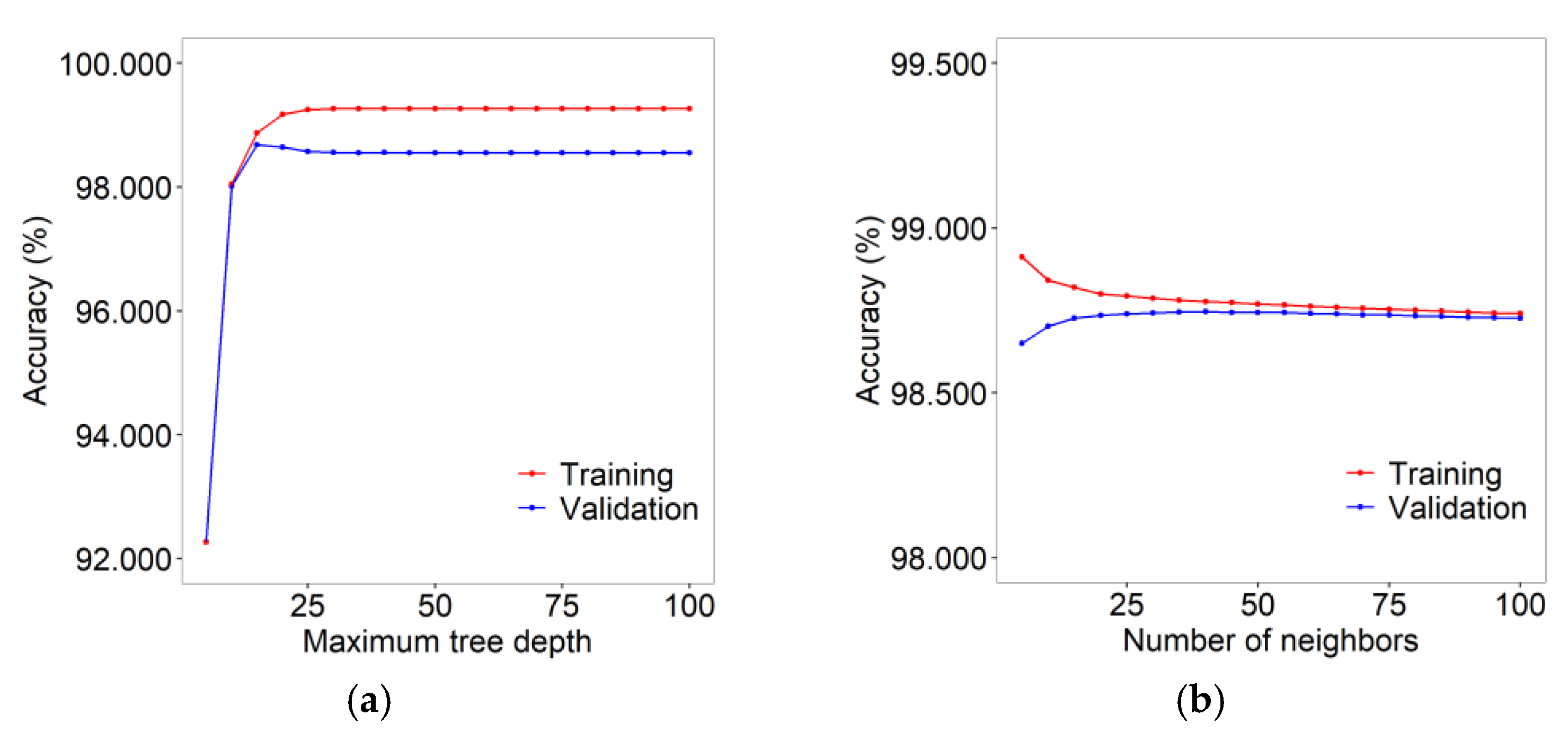
Hyperparameters in both RF and KNN were tuned in order to balance the performance on both the training and validation data sets. The average OA of RF models from stratified 5-fold cross-validation during model development are shown in Figure 5a. The maximum depth of the tree of 15 was selected for the optimal RF model as it led to the highest average validation accuracy of 98.579%. The selection of an optimal k for the KNN model is shown in Figure 5b. The average validation accuracy from stratified 5-fold cross-validation peaked at 98.651% when k = 35.
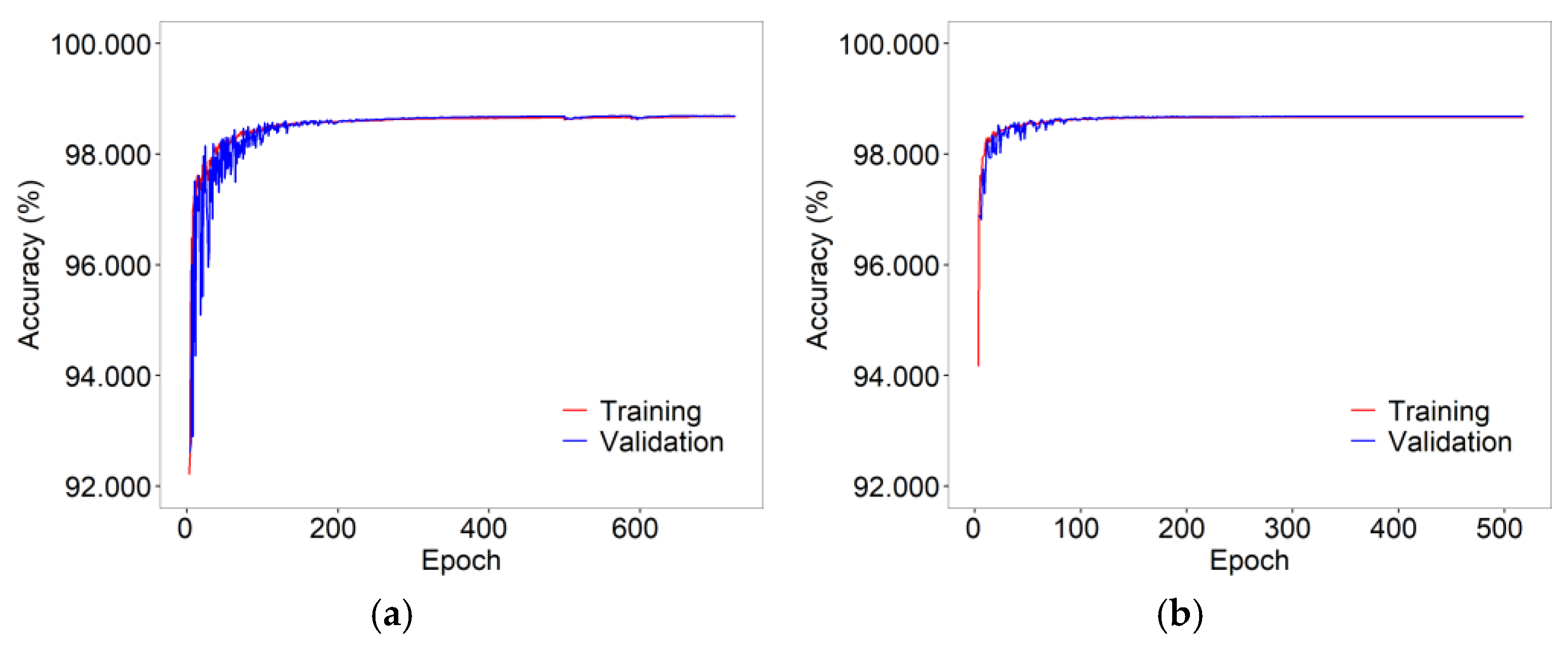
Both 1DTransformer and 1DCNN were designed to include skip concatenation to make full use of different levels of features for the classification. The 1DCNN model had faster convergence speed, which took 375 epochs (Figure 6a) to reach the plateau, while 1DTransformer took 587 epochs (Figure 6b).
Both the ML and DL models with the highest validation accuracies (Table 2) in stratified 5-fold cross-validations were selected as the best performing ones and further developed to check their performances on the independent ground truth test data set. Regardless of the small margin in performances among all four models, 1DTransformer had the highest OA, followed by 1DCNN and KNN. RF had the lowest OA during validation among the four models.
3.2. Ablation Study on Transformer Model
No skip concatenation was included in classical transformer models, while it was added in this study to reuse the lower-level features for classification. The 1DTransformer without skip concatenation had worse performance, with lower values in all evaluation metrics, in this study (Table 2).
3.3. Inference Speed
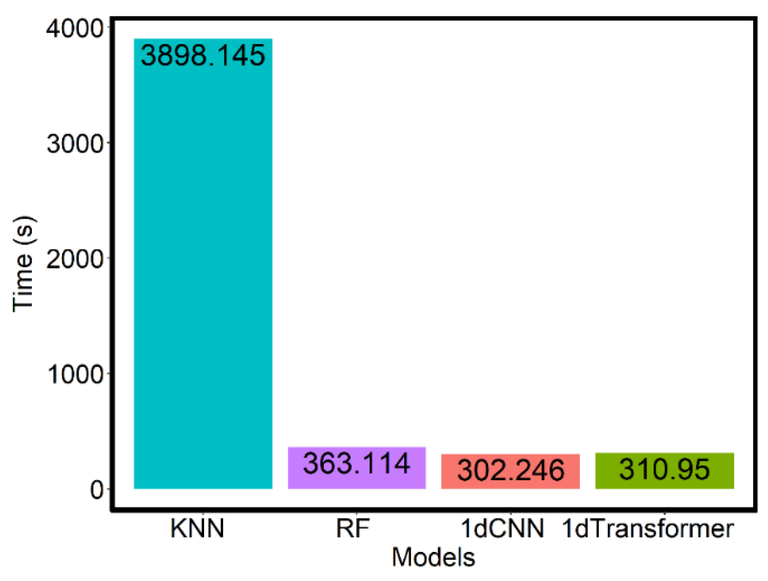
The inference speed of each model is shown in Figure 7. Model KNN had the lowest speed, which was 3898.145 s to classify a 203.574 million pixel image. The other three models had very similar and higher speeds: 363.114 s (RF), 310.95 s (1DTransformer), and 302.246 s (1DCNN), respectively.
3.4. Model Testing against Ground Reference Data
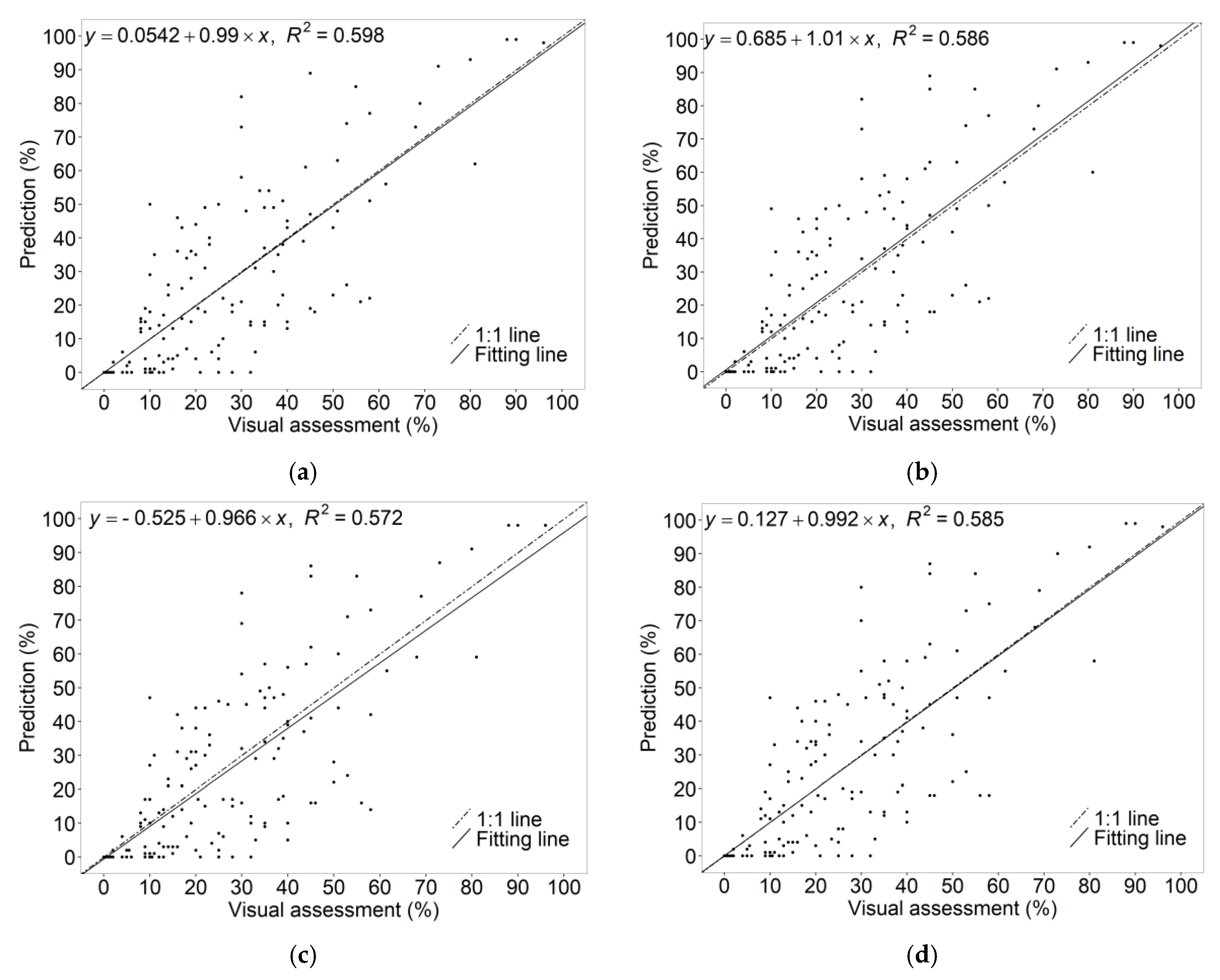
The testing performances of different models had the same trend as their OAs on the validation dataset. The model 1DTransformer was able to maintain the best performance with the highest R2 value of 0.598 (Figure 8a). Both 1DCNN and KNN shared very similar R2 values, 0.586 (Figure 8b) and 0.585 (Figure 8d), respectively. RF had the lowest R2 of 0.572 (Figure 8c) on the testing data.
3.5. Weed Maps
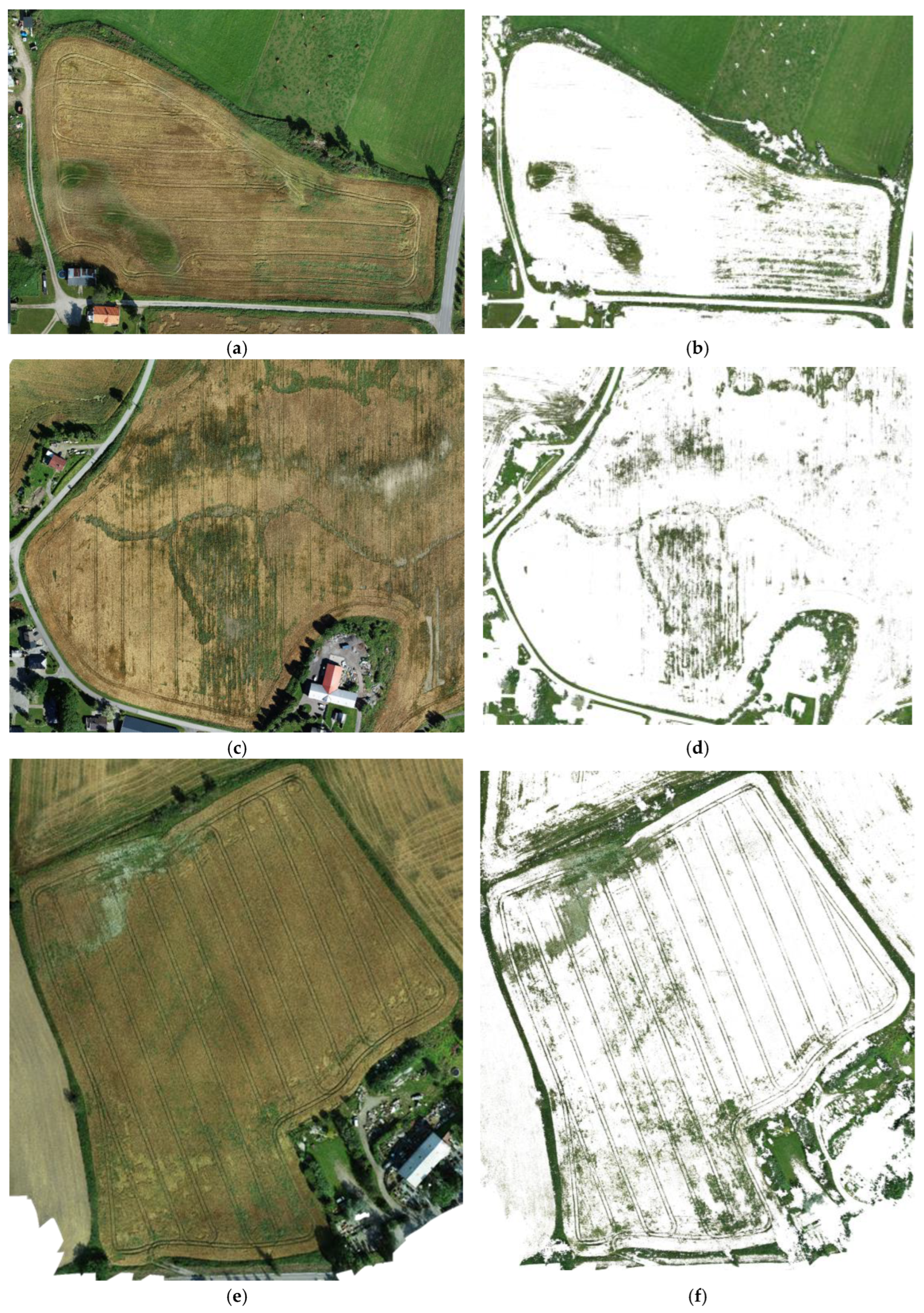
Examples of weed maps of three representative fields based on predictions from the 1DTransformer model are shown in Figure 9. Most of the within-field weeds which were green were segmented effectively by the model. Surprisingly, weeds that had colors other than green were also separated clearly by the model, although this result was based on visual evaluation only (the bottom row of Figure 9).
4. Discussion
Most state-of-the-art weed detection or segmentation tasks are performed in 2D space; however, these detection or segmentation models require clearly annotated 2D images at the pixel level. For example, for weed coverage estimation, at least all the pixels belonging to weeds must be annotated, which is often infeasible or rather labor-intensive to perform. Moreover, annotating imagery at lower spatial resolutions, as with the UAV imagery in this study, often leads to incorrect annotations of pixels due to a mix of spectral signals from multiple objects being projected onto a single pixel element. Through sampling representative pixels of each class, the data preparation process became much easier and DL models could still be developed to classify 1D pixels of weeds, crops, and other with high accuracies.
The suggested 1DTransformer model is a new DL method to map arable weeds based on UAV images. The optimal model selected had high fidelity in predicting weed pixels and the ground reference weed coverage in the field, proving the soundness of OA in selecting more robust models. Its high performances in both validation and testing could be partially attributed to the more effective feature extraction mechanism of attention-based models compared to CNN [45]. Attention, as the core of a transformer model, has been shown to be more effective in feature extraction and achieved better model performances in different tasks in computer vision and language models [45], and once more proved to be more effective, even when working solely on color information, compared to a CNN model. The attention in a transformer model aggregates global information from all three color channels simultaneously to reach a higher accuracy, while the receptive field in CNN is limited by the window size.
Besides the attention mechanism itself, we also confirmed the benefits of having skip concatenation in the model. The skip concatenation has shown to be useful in multiple studies before, either in multilayer perceptron (MLP) or CNN [57,58]. The concatenation of high- and low-level features solves the problems of vanishing gradient and encouraging feature reuse and propagation [59], and accordingly accumulates as much useful information as possible to allow the model to reach a better performance. The large data set we collected (0.765 million pixels) might also be responsible for the slightly better performance of the 1DTransformer compared to 1DCNN. Transformer models have proved to have better performance on larger data sets [40].
Classical ML methods have been popular in image-based weed detection and mapping [26]. However, there is a claim that ML models generally do not work well on raw RGB imagery, and their performances rely heavily on the hand-crafted features prepared based on prior knowledge [60]. Feature selection must be carried out as an additional step for classical ML models in order to reduce the risks caused by the ‘curse of dimensionality’ [61]. To our surprise, our KNN-based model almost reached the same performance as the 1DCNN model based on raw RGB pixels. This was in agreement with Forero et al. (2019) who found very similar performance between a neural network (unspecified) and five ML models in predicting thistles (C. arvense) in ripe cereals. The huge gap between classical ML and DL models observed in other studies could be due to their much higher spatial resolution UAV imagery (through flying a UAV 6 m above the field) or a more effective DL model used [35]. Moreover, our late-season monitoring could be another reason for the small performance difference between the DL and classical ML models. With late-season monitoring, there was a relatively clear color contrast between crops and the target weed species.
Regardless of the consistency in performances of all four models in both validation and testing, the large performance drop during testing on the ground reference data were noticeable in all models (cf. Figure 7). Unavoidable subjective bias from different observers, different years, and different crop heights are likely sources for the low accuracies. Furthermore, the sampled pixels for model building were mainly from relatively “pure” pixels in order to avoid ambiguities. Previous models trained on pure pixels have had problems in predicting pixels with mixed classes [62]. Other reasons could be the differences in view angle and spatial resolution for the UAV imagery and ground reference data. UAV imagery was taken nadir and at high altitudes (resulting in around 33 mm g.s.d.), whereas observers were about 1 m away from the evaluation plots, estimating weed coverage at an oblique view for an entire plot (about 16 m2). Rasmussen et al. (2019) found that their threshold-based VI model for RGB UAV imagery (‘Thistle Tool’) overestimated the area of thistles (C. arvense) compared to visual scoring in the field. They explained the discrepancy by the fact that nadir view images could detect weeds beneath crop canopy while observers could not see them from their view angle. When the same observers assessed weed cover in the orthomosaics, the regression line was close to the 1:1 line (Rasmussen et al., 2019). Thistles are difficult to assess visually in the field because many shoots are shorter than the senescent cereal crop canopy [63].
Our model is intended for pre-harvest mapping of weeds in cereals fields known to be infested by creeping perennial weed species. Green vegetation at the margins outside the fields will also be detected as weeds (cf. Figure 8). With field boundary masks, this apparent error is easily solved. The model can be the basis for SSWM, either before the crop harvest, spraying glyphosate (if legal), after the harvest, or in the next crop using herbicides or non-chemical measures. The model should be applicable in practice because patches that are more susceptible to weed infestation are relatively consistent each year [64,65]. One additional application of the model is estimation of weed control efficacy in large-scale field trials on weed control measures, as recently shown [66,67]. In any SSWM purpose, the raw weed map needs to be translated into a prescription map, taking the spatial resolution of the weeding machinery into account. Furthermore, buffer pixels around predicted weedy pixels should also be added to avoid leaving weeds untreated [23], especially if the weed management takes place weeks or months after the UAV flight. If applied on fields with other weed types as well and which are clearly visible above the canopy at the time of imaging, the model is not capable of separating the weed types, nor tramlines if they contain non-mature crop plants. Both are clearly illustrated in Figure 9e,f. Scentless mayweed (Tripleurospermum inodorum) was flowering (white flowers) in a large patch in the NW part of this field at the time of UAV imaging and was predicted as ‘weeds’. This was expected since the model was developed on a dataset where weeds pixels were sampled regardless of color, although the majority were green. It also proved the advantage of learning-based models that are more robust in practical usage in comparison to index-based thresholding ones.
The performance of 1Dtransformer models have generally been less studied compared to its 2D counterpart [47,48] and other CNN-based models. Our study proved its slight superiority in classifying weeds (mainly greenish), small-grain crops (mainly yellowish), and ‘other’, as well as estimating total weed coverage in sub-field plots. This study paves the road for more effective DL applications in precision agriculture in the future, especially when image resolution is not high enough and it is hard to get high-quality training data. Additionally, the inference speed and model performance were more balanced compared to other models, which make 1DTransformer even more advantageous in practical SSWM applications. These potentially more effective DL models should be applied to facilitate SSWM in order to reduce the risks associated with herbicides and weeding measures based on soil disturbance.
5. Conclusions
We accurately used a 1D transformer DL model to perform pixel-wise classification on weeds, late-season small-grain cereals, and ‘other’ in easily accessible low-spatial-resolution UAV RGB imagery. The developed 1DTransformer model was shown to be a robust classifier that generalizes well under realistic field and weather conditions across multiple years, weed compositions, and cereal species. The 1DCNN model was characterized by a slightly higher inference speed than the 1DTransformer model in weed mapping, both of which were faster than two classical KNN and RF models. The balanced performance of inference speed and classification accuracy made 1DTransformer favorable in practical SSWM applications.
Author Contributions
Conceptualization, T.W.B. and J.G.; methodology, formal analysis and original draft preparation, J.Z.; review and editing, T.W.B. and J.G. All authors have read and agreed to the published version of the manuscript.
Funding
The study was part of the ‘PRESIS project’ funded by the Norwegian Partners of the Agricultural Settlement Fund (‘Avtalepartene i jordbruksoppgjøret’), grant No. 159205 (“Presisjonsjordbruk ut i praksis—forskningsbasert utvikling og kvalitetssikring av klimavennlige tjenester som er lønnsomme for bonden”).
Data Availability Statement
Data is available upon request.
Acknowledgments
We acknowledge our NIBIO colleagues K. Wærnhus, A. M. Beachell, M. Helgheim, J. Ødegaard, and M. B. Fajardo, for assisting in field work, M. L. Græsdahl, K. Rindal, and M. Pircher for planning and conducting the UAV flight missions, and M. Bordbarkhoo for processing the UAV imagery to orthomosaics. We also thank Å. Langeland, Norwegian Extension Service, for suggesting relevant fields, and all the grain producers for providing fields for this research.
Conflicts of Interest
The authors declare no conflict of interest.
References
- Rew, L.J.; Cussans, G.W.; Mugglestone, M.A.; Miller, P.C.H. A Technique for Mapping the Spatial Distribution of Elymus Repots, with Estimates of the Potential Reduction in Herbicide Usage from Patch Spraying. Weed Res. 1996, 36, 283–292. [Google Scholar] [CrossRef]
- Hamouz, P.; Hamouzová, K.; Holec, J.; Tyšer, L. Impact of Site-Specific Weed Management on Herbicide Savings and Winter Wheat Yield. Plant Soil. Environ. 2013, 59, 101–107. [Google Scholar] [CrossRef]
- Blank, L.; Rozenberg, G.; Gafni, R. Spatial and Temporal Aspects of Weeds Distribution within Agricultural Fields–A Review. Crop Prot. 2023, 106300. [Google Scholar] [CrossRef]
- Fernández-Quintanilla, C.; Peña, J.M.; Andújar, D.; Dorado, J.; Ribeiro, A.; López-Granados, F. Is the Current State of the Art of Weed Monitoring Suitable for Site-specific Weed Management in Arable Crops? Weed Res. 2018, 58, 259–272. [Google Scholar] [CrossRef]
- Timmermann, C.; Gerhards, R.; Kühbauch, W. The Economic Impact of Site-Specific Weed Control. Precis. Agric. 2003, 4, 249–260. [Google Scholar] [CrossRef]
- López-Granados, F.; Torres-Sánchez, J.; Serrano-Pérez, A.; de Castro, A.I.; Mesas-Carrascosa, F.-J.; Peña, J.-M. Early Season Weed Mapping in Sunflower Using UAV Technology: Variability of Herbicide Treatment Maps against Weed Thresholds. Precis. Agric. 2016, 17, 183–199. [Google Scholar] [CrossRef]
- Castaldi, F.; Pelosi, F.; Pascucci, S.; Casa, R. Assessing the Potential of Images from Unmanned Aerial Vehicles (UAV) to Support Herbicide Patch Spraying in Maize. Precis. Agric. 2017, 18, 76–94. [Google Scholar] [CrossRef]
- Coleman, G.R.Y.; Bender, A.; Hu, K.; Sharpe, S.M.; Schumann, A.W.; Wang, Z.; Bagavathiannan, M.V.; Boyd, N.S.; Walsh, M.J. Weed Detection to Weed Recognition: Reviewing 50 Years of Research to Identify Constraints and Opportunities for Large-Scale Cropping Systems. Weed Technol. 2022, 36, 741–757. [Google Scholar] [CrossRef]
- Barroso, J.; San Martin, C.; McCallum, J.D.; Long, D.S. Economic and Management Value of Weed Maps at Harvest in Semi-Arid Cropping Systems of the US Pacific Northwest. Precis. Agric. 2021, 22, 1936–1951. [Google Scholar] [CrossRef]
- Gerhards, R.; Andujar Sanchez, D.; Hamouz, P.; Peteinatos, G.G.; Christensen, S.; Fernandez-Quintanilla, C. Advances in Site-specific Weed Management in Agriculture—A Review. Weed Res. 2022, 62, 123–133. [Google Scholar] [CrossRef]
- Sapkota, R.; Stenger, J.; Ostlie, M.; Flores, P. Towards Reducing Chemical Usage for Weed Control in Agriculture Using UAS Imagery Analysis and Computer Vision Techniques. Sci. Rep. 2023, 13, 6548. [Google Scholar] [CrossRef] [PubMed]
- Coleman, G.R.Y.; Stead, A.; Rigter, M.P.; Xu, Z.; Johnson, D.; Brooker, G.M.; Sukkarieh, S.; Walsh, M.J. Using Energy Requirements to Compare the Suitability of Alternative Methods for Broadcast and Site-Specific Weed Control. Weed Technol. 2019, 33, 633–650. [Google Scholar] [CrossRef]
- Christensen, S.; Søgaard, H.T.; Kudsk, P.; Nørremark, M.; Lund, I.; Nadimi, E.S.; Jørgensen, R. Site-specific Weed Control Technologies. Weed Res. 2009, 49, 233–241. [Google Scholar] [CrossRef]
- Peteinatos, G.G.; Weis, M.; Andújar, D.; Rueda Ayala, V.; Gerhards, R. Potential Use of Ground-based Sensor Technologies for Weed Detection. Pest. Manag. Sci. 2014, 70, 190–199. [Google Scholar] [CrossRef] [PubMed]
- Lati, R.N.; Rasmussen, J.; Andujar, D.; Dorado, J.; Berge, T.W.; Wellhausen, C.; Pflanz, M.; Nordmeyer, H.; Schirrmann, M.; Eizenberg, H. Site-specific Weed Management—Constraints and Opportunities for the Weed Research Community: Insights from a Workshop. Weed Res. 2021, 61, 147–153. [Google Scholar] [CrossRef]
- Barroso, J.; Ruiz, D.; Fernandez-Quintanilla, C.; Leguizamon, E.S.; Hernaiz, P.; Ribeiro, A.; Díaz, B.; Maxwell, B.D.; Rew, L.J. Comparison of Sampling Methodologies for Site-specific Management of Avena Sterilis. Weed Res. 2005, 45, 165–174. [Google Scholar] [CrossRef]
- Shahbazi, N.; Ashworth, M.B.; Callow, J.N.; Mian, A.; Beckie, H.J.; Speidel, S.; Nicholls, E.; Flower, K.C. Assessing the Capability and Potential of LiDAR for Weed Detection. Sensors 2021, 21, 2328. [Google Scholar] [CrossRef]
- Islam, N.; Rashid, M.M.; Wibowo, S.; Xu, C.-Y.; Morshed, A.; Wasimi, S.A.; Moore, S.; Rahman, S.M. Early Weed Detection Using Image Processing and Machine Learning Techniques in an Australian Chilli Farm. Agriculture 2021, 11, 387. [Google Scholar] [CrossRef]
- Xia, F.; Quan, L.; Lou, Z.; Sun, D.; Li, H.; Lv, X. Identification and Comprehensive Evaluation of Resistant Weeds Using Unmanned Aerial Vehicle-Based Multispectral Imagery. Front. Plant Sci. 2022, 13, 938604. [Google Scholar] [CrossRef]
- Esposito, M.; Crimaldi, M.; Cirillo, V.; Sarghini, F.; Maggio, A. Drone and Sensor Technology for Sustainable Weed Management: A Review. Chem. Biol. Technol. Agric. 2021, 8, 1–11. [Google Scholar] [CrossRef]
- Yang, W.; Wang, S.; Zhao, X.; Zhang, J.; Feng, J. Greenness Identification Based on HSV Decision Tree. Inf. Process. Agric. 2015, 2, 149–160. [Google Scholar] [CrossRef]
- Anderegg, J.; Tschurr, F.; Kirchgessner, N.; Treier, S.; Schmucki, M.; Streit, B.; Walter, A. On-Farm Evaluation of UAV-Based Aerial Imagery for Season-Long Weed Monitoring under Contrasting Management and Pedoclimatic Conditions in Wheat. Comput. Electron. Agric. 2023, 204, 107558. [Google Scholar] [CrossRef]
- Rasmussen, J.; Nielsen, J.; Streibig, J.C.; Jensen, J.E.; Pedersen, K.S.; Olsen, S.I. Pre-Harvest Weed Mapping of Cirsium arvense in Wheat and Barley with off-the-Shelf UAVs. Precis. Agric. 2019, 20, 983–999. [Google Scholar] [CrossRef]
- Hamouz, P.; Hamouzová, K.; Soukup, J. Detection of Cirsium arvense L. in Cereals Using a Multispectral Imaging and Vegetation Indices. Herbologia 2009, 10, 41–48. [Google Scholar]
- Liu, B.; Bruch, R. Weed Detection for Selective Spraying: A Review. Curr. Robot. Rep. 2020, 1, 19–26. [Google Scholar] [CrossRef]
- Wang, A.; Zhang, W.; Wei, X. A Review on Weed Detection Using Ground-Based Machine Vision and Image Processing Techniques. Comput. Electron. Agric. 2019, 158, 226–240. [Google Scholar] [CrossRef]
- Ahmed, F.; Al-Mamun, H.A.; Bari, A.S.M.H.; Hossain, E.; Kwan, P. Classification of Crops and Weeds from Digital Images: A Support Vector Machine Approach. Crop Prot. 2012, 40, 98–104. [Google Scholar] [CrossRef]
- Su, J.; Yi, D.; Coombes, M.; Liu, C.; Zhai, X.; McDonald-Maier, K.; Chen, W.-H. Spectral Analysis and Mapping of Blackgrass Weed by Leveraging Machine Learning and UAV Multispectral Imagery. Comput. Electron. Agric. 2022, 192, 106621. [Google Scholar] [CrossRef]
- Gašparović, M.; Zrinjski, M.; Barković, Đ.; Radočaj, D. An Automatic Method for Weed Mapping in Oat Fields Based on UAV Imagery. Comput. Electron. Agric. 2020, 173, 105385. [Google Scholar] [CrossRef]
- Alahmari, F.; Naim, A.; Alqahtani, H. E-Learning Modeling Technique and Convolution Neural Networks in Online Education. In IoT-Enabled Convolutional Neural Networks: Techniques and Applications; River Publishers: Aalborg, Denmark, 2023; pp. 261–295. [Google Scholar]
- Krichen, M. Convolutional Neural Networks: A Survey. Computers 2023, 12, 151. [Google Scholar] [CrossRef]
- Ofori, M.; El-Gayar, O.F. Towards Deep Learning for Weed Detection: Deep Convolutional Neural Network Architectures for Plant Seedling Classification. In Proceedings of the AMCIS 2020 Conference, Salt Lake City, UT, USA, 10–14 August 2020. [Google Scholar]
- LeCun, Y.; Bengio, Y.; Hinton, G. Deep Learning. Nature 2015, 521, 436–444. [Google Scholar] [CrossRef] [PubMed]
- Hashemi-Beni, L.; Gebrehiwot, A.; Karimoddini, A.; Shahbazi, A.; Dorbu, F. Deep Convolutional Neural Networks for Weeds and Crops Discrimination from UAS Imagery. Front. Remote Sens. 2022, 3, 1. [Google Scholar] [CrossRef]
- Xu, K.; Shu, L.; Xie, Q.; Song, M.; Zhu, Y.; Cao, W.; Ni, J. Precision Weed Detection in Wheat Fields for Agriculture 4.0: A Survey of Enabling Technologies, Methods, and Research Challenges. Comput. Electron. Agric. 2023, 212, 108106. [Google Scholar] [CrossRef]
- Huang, H.; Lan, Y.; Deng, J.; Yang, A.; Deng, X.; Zhang, L.; Wen, S. A Semantic Labeling Approach for Accurate Weed Mapping of High Resolution UAV Imagery. Sensors 2018, 18, 2113. [Google Scholar] [CrossRef] [PubMed]
- Fawakherji, M.; Youssef, A.; Bloisi, D.; Pretto, A.; Nardi, D. Crop and Weeds Classification for Precision Agriculture Using Context-Independent Pixel-Wise Segmentation. In Proceedings of the Third IEEE International Conference on Robotic Computing (IRC), Naples, Italy, 25–27 February 2019; pp. 146–152. [Google Scholar]
- Milioto, A.; Lottes, P.; Stachniss, C. Real-Time Semantic Segmentation of Crop and Weed for Precision Agriculture Robots Leveraging Background Knowledge in CNNs. In Proceedings of the IEEE International Conference on Robotics and Automation (ICRA), Brisbane, Australia, 21–25 May 2018; pp. 2229–2235. [Google Scholar]
- Lameski, P.; Zdravevski, E.; Trajkovik, V.; Kulakov, A. Weed Detection Dataset with RGB Images Taken under Variable Light Conditions. In ICT Innovations 2017: Data-Driven Innovation, Proceedings of the 9th International Conference, ICT Innovations 2017, Skopje, Macedonia, 18–23 September 2017, Proceedings 9; Springer: Berlin/Heidelberg, Germany, 2017; pp. 112–119. [Google Scholar]
- Fraccaro, P.; Butt, J.; Edwards, B.; Freckleton, R.P.; Childs, D.Z.; Reusch, K.; Comont, D. A Deep Learning Application to Map Weed Spatial Extent from Unmanned Aerial Vehicles Imagery. Remote Sens. 2022, 14, 4197. [Google Scholar] [CrossRef]
- Liu, Z.; Lin, Y.; Cao, Y.; Hu, H.; Wei, Y.; Zhang, Z.; Lin, S.; Guo, B. Swin Transformer: Hierarchical Vision Transformer Using Shifted Windows. In Proceedings of the IEEE/CVF International Conference on Computer Vision, Montreal, BC, Canada, 11–17 October 2021; pp. 10012–10022. [Google Scholar]
- Xie, E.; Wang, W.; Yu, Z.; Anandkumar, A.; Alvarez, J.M.; Luo, P. SegFormer: Simple and Efficient Design for Semantic Segmentation with Transformers. Adv. Neural Inf. Process Syst. 2021, 34, 12077–12090. [Google Scholar]
- Strudel, R.; Garcia, R.; Laptev, I.; Schmid, C. Segmenter: Transformer for Semantic Segmentation. In Proceedings of the IEEE/CVF International Conference on Computer Vision, Montreal, BC, Canada, 11–17 October 2021; pp. 7262–7272. [Google Scholar]
- Horwath, J.P.; Zakharov, D.N.; Mégret, R.; Stach, E.A. Understanding Important Features of Deep Learning Models for Segmentation of High-Resolution Transmission Electron Microscopy Images. NPJ Comput. Mater. 2020, 6, 108. [Google Scholar] [CrossRef]
- Bosilj, P.; Aptoula, E.; Duckett, T.; Cielniak, G. Transfer Learning between Crop Types for Semantic Segmentation of Crops versus Weeds in Precision Agriculture. J. Field Robot. 2020, 37, 7–19. [Google Scholar] [CrossRef]
- Dosovitskiy, A.; Beyer, L.; Kolesnikov, A.; Weissenborn, D.; Zhai, X.; Unterthiner, T.; Dehghani, M.; Minderer, M.; Heigold, G.; Gelly, S. An Image Is Worth 16x16 Words: Transformers for Image Recognition at Scale. arXiv 2020, arXiv:2010.11929. [Google Scholar]
- Reedha, R.; Dericquebourg, E.; Canals, R.; Hafiane, A. Transformer Neural Network for Weed and Crop Classification of High Resolution UAV Images. Remote Sens. 2022, 14, 592. [Google Scholar] [CrossRef]
- Liang, J.; Wang, D.; Ling, X. Image Classification for Soybean and Weeds Based on VIT. Proc. J. Phys. Conf. Ser. 2021, 2002, 12068. [Google Scholar] [CrossRef]
- Jiang, K.; Afzaal, U.; Lee, J. Transformer-Based Weed Segmentation for Grass Management. Sensors 2023, 23, 65. [Google Scholar] [CrossRef] [PubMed]
- Forbord, M.; Vik, J. Food, Farmers, and the Future: Investigating Prospects of Increased Food Production within a National Context. Land Use Policy 2017, 67, 546–557. [Google Scholar] [CrossRef]
- Breiman, L. Random Forests. Mach. Learn. 2001, 45, 5–32. [Google Scholar] [CrossRef]
- Altman, N.S. An Introduction to Kernel and Nearest-Neighbor Nonparametric Regression. Am. Stat. 1992, 46, 175–185. [Google Scholar]
- Ma, X.; Deng, X.; Qi, L.; Jiang, Y.; Li, H.; Wang, Y.; Xing, X. Fully Convolutional Network for Rice Seedling and Weed Image Segmentation at the Seedling Stage in Paddy Fields. PLoS ONE 2019, 14, e0215676. [Google Scholar] [CrossRef] [PubMed]
- Thanh Noi, P.; Kappas, M. Comparison of Random Forest, k-Nearest Neighbor, and Support Vector Machine Classifiers for Land Cover Classification Using Sentinel-2 Imagery. Sensors 2017, 18, 18. [Google Scholar] [CrossRef] [PubMed]
- Buitinck, L.; Louppe, G.; Blondel, M.; Pedregosa, F.; Mueller, A.; Grisel, O.; Niculae, V.; Prettenhofer, P.; Gramfort, A.; Grobler, J. API Design for Machine Learning Software: Experiences from the Scikit-Learn Project. arXiv 2013, arXiv:1309.0238. [Google Scholar]
- Ali, J.; Khan, R.; Ahmad, N.; Maqsood, I. Random Forests and Decision Trees. Int. J. Comput. Sci. 2012, 9, 272. [Google Scholar]
- Chicco, D.; Warrens, M.J.; Jurman, G. The Coefficient of Determination R-Squared Is More Informative than SMAPE, MAE, MAPE, MSE and RMSE in Regression Analysis Evaluation. PeerJ. Comput. Sci. 2021, 7, e623. [Google Scholar] [CrossRef]
- Zhao, J.; Qu, Y.; Ninomiya, S.; Guo, W. Endmember-Assisted Camera Response Function Learning, Toward Improving Hyperspectral Image Super-Resolution Performance. IEEE Trans. Geosci. Remote Sens. 2022, 60, 1–14. [Google Scholar] [CrossRef]
- Zhao, J.; Kaga, A.; Yamada, T.; Komatsu, K.; Hirata, K.; Kikuchi, A.; Hirafuji, M.; Ninomiya, S.; Guo, W. Improved Field-Based Soybean Seed Counting and Localization with Feature Level Considered. Plant Phenomics 2023, 5, 26. [Google Scholar] [CrossRef] [PubMed]
- Huang, G.; Liu, Z.; Van Der Maaten, L.; Weinberger, K.Q. Densely Connected Convolutional Networks. In Proceedings of the IEEE Conference on Computer Vision and Pattern Recognition, Honolulu, HI, USA, 21–26 July 2017; pp. 4700–4708. [Google Scholar]
- Janiesch, C.; Zschech, P.; Heinrich, K. Machine Learning and Deep Learning. Electron. Mark. 2021, 31, 685–695. [Google Scholar] [CrossRef]
- Onishi, M.; Ise, T. Explainable Identification and Mapping of Trees Using UAV RGB Image and Deep Learning. Sci. Rep. 2021, 11, 903. [Google Scholar] [CrossRef] [PubMed]
- Fu, Y.; Zheng, Y.; Zhang, L.; Zheng, Y.; Huang, H. Simultaneous Hyperspectral Image Super-Resolution and Geometric Alignment with a Hybrid Camera System. Neurocomputing 2020, 384, 282–294. [Google Scholar] [CrossRef]
- Rasmussen, J.; Azim, S.; Nielsen, J. Pre-Harvest Weed Mapping of Cirsium arvense L. Based on Free Satellite Imagery–The Importance of Weed Aggregation and Image Resolution. Eur. J. Agron. 2021, 130, 126373. [Google Scholar] [CrossRef]
- Heijting, S.; Van Der Werf, W.; Stein, A.; Kropff, M.J. Are Weed Patches Stable in Location? Application of an Explicitly Two-dimensional Methodology. Weed Res. 2007, 47, 381–395. [Google Scholar] [CrossRef]
- Oerke, E.-C.; Gerhards, R.; Menz, G.; Sikora, R.A. Precision Crop Protection-the Challenge and Use of Heterogeneity; Springer: Berlin/Heidelberg, Germany, 2010; Volume 5. [Google Scholar]
- Weigel, M.M.; Andert, S.; Gerowitt, B. Monitoring Patch Expansion Amends to Evaluate the Effects of Non-Chemical Control on the Creeping Perennial Cirsium arvense (L.) Scop. in a Spring Wheat Crop. Agronomy 2023, 13, 1474. [Google Scholar] [CrossRef]
Figure 1.
Ground reference data on weed coverage. Sub-field area of an original UAV orthomosaic (a), three sampling plots (16 m2) for ground reference data masked as red polygons (b), and a ground-based photo of another exemplary plot containing thistles (Cirsium arvense) with the plot’s corners marked by white styrofoam balls (c).

Figure 2.
Manually selected pixels (white) of weeds (a), crops (b), and other (c) in an example orthomosaic.
Figure 2.
Manually selected pixels (white) of weeds (a), crops (b), and other (c) in an example orthomosaic.

Figure 3.
The architecture of the 1DTransformer (a), skip concatenation (b), and transformer encoder (c). “Concat” means the features are concatenated while “+” means the features are added. “Fc” stands for a fully connected layer; “Norm” means layer-wise normalization. The “n” stands for the number of pixels and channel is the feature dimension of input image; “Class” is the number of output classes, representing crops, weeds, and other.

Figure 4.
The architecture of the 1DCNN. “Conv1” in (a) is a convolution layer with kernel size = 1; “Fc” is a fully connected layer. Skip concatenation is shown in (b) with kernel size = 2 in each Conv layer. “Concat” means the features are concatenated while “+” means the features are added. The “n” stands for the number of pixels and “channel” is the feature dimension of input image; “class” is the number of output classes, representing crops, weeds, and other.

Figure 5.
Hyperparameter tuning of RF and KNN. Maximum tree depth was tuned for RF (a) and number of neighbors were tuned for KNN (b).
Figure 5.
Hyperparameter tuning of RF and KNN. Maximum tree depth was tuned for RF (a) and number of neighbors were tuned for KNN (b).

Figure 6.
Training histories of 1DTransformer (a) and 1DCNN (b).

Figure 7.
Inference speed of the different models on the same orthomosaic with 203.574 million pixels.
Figure 7.
Inference speed of the different models on the same orthomosaic with 203.574 million pixels.

Figure 8.
Simple linear regressions of weed coverage predictions from the best performing 1DTransformer (a), 1DCNN (b), RF (c), and KNN (d), with the ground reference data on total weed coverage per plot (134 plots sized 4 m by 4 m across 15 cereal fields).
Figure 8.
Simple linear regressions of weed coverage predictions from the best performing 1DTransformer (a), 1DCNN (b), RF (c), and KNN (d), with the ground reference data on total weed coverage per plot (134 plots sized 4 m by 4 m across 15 cereal fields).

Figure 9.
Examples of original UAV image (a,c,e) and predicted output weed map (b,d,f) with the cereal crop masked (white pixels) using the DL model 1DTransformer. Green vegetation outside the cereal fields was also detected as weeds.
Figure 9.
Examples of original UAV image (a,c,e) and predicted output weed map (b,d,f) with the cereal crop masked (white pixels) using the DL model 1DTransformer. Green vegetation outside the cereal fields was also detected as weeds.


Table 1.
Overview of the fields used in the study.
| Field | ID | Crop Species | Ground Reference Data | Perennial Weed Species | Annual (Biennial) Weed Species | UAV Flight * |
|---|---|---|---|---|---|---|
| 1 | Aas | Barley (2-row) | 06.08.2020 | Elymus repens | Viola arvensis | 06.08.2020 (0) |
| 2 | Vestby | Barley (2-row) | 06.08.2020 | E. repens | Poa annua | 06.08.2020 (0) |
| 3 | Frogn | Barley (2-row) | 06.08.2020 | E. repens | V. arvensis | 06.08.2020 (0) |
| 4 | Blaestad | Barley | 10.08.2020 | E. repens | P. annua, V. arvensis | 11.08.2020 (1) |
| 5 | Aalstad_1 | Barley | 11.08.2020 | Cirsium arvense | P. annua | 11.08.2020 (0) |
| 6 | Aalstad_2 | Barley | 12.08.2020 | C. arvense | P. annua | 11.08.2020 (1) |
| 7 | Krogsrud | Wheat (spring) | 05.08.2021 | E. repens (Artemisia vulgaris, C. arvense) | P. annua | 10.08.2021 (5) |
| 8 | Roed | Oat | 05.08.2021 | C. arvense (Mentha sp.) | (Not registered) | 10.08.2021 (5) |
| 9 | Krukkegaarden | Barley | 05.08.2021 | E. repens (C. arvense) | Tripleurospermum inodorum | 10.08.2021 (5) |
| 10 | Sinnerud | Barley | 09.08.2021 | E. repens, C. arvense, A. vulgaris | Erodium cicutarium, Sonchus asper | 11.08.2021 (2) |
| 11 | Soerum | Wheat (spring) | 09.08.2021 | E. repens, C. arvense (Vicia cracca) | Capsella bursa-pastoris, Persicaria maculosa, P. annua | 11.08.2021 (2) |
| 12 | Vestad | Barley | 09.08.2021 | E. repens, C. arvense, Sonchus arvensis | Stellaria media, Polygonum aviculare, P. annua, Fumaria officinalis, S. asper | 11.08.2021 (2) |
| 13 | Olstad | Barley (6-row) | 01.08.2022 | C. arvense (E. repens) | V. arvensis, F. officinalis, T. inodorum, S. asper, S. media, P. aviculare, vol. wheat | 05.08.2022 (4) |
| 14 | Soeraas | Wheat (winter) | 08.08.2022 | C. arvense, S. arvensis, E. repens, Stachys palustris (A. vulgaris) | Chenopodium album, S. asper | 10.08.2022 (2) |
| 15 | Tomte | Barley (6-row) | 22.08.2022 | E. repens (C. arvense) | (Not registered) | 25.08.2022 (3) |
* In brackets the number of days before or after the ground reference data were sampled.
Table 2.
Evaluation metrics on sampled pixels from stratified 5-fold cross-validation during model development *.
Table 2.
Evaluation metrics on sampled pixels from stratified 5-fold cross-validation during model development *.
| Model | OA (%) | Precision (%) | Recall (%) | F1-score | ||||||
|---|---|---|---|---|---|---|---|---|---|---|
| Weed | Crop | Other | Weed | Crop | Other | Weed | Crop | Other | ||
| KNN | 98.669 | 98.915 | 98.296 | 98.957 | 97.472 | 98.821 | 98.675 | 0.98188 | 0.98558 | 0.98816 |
| RF | 98.600 | 99.163 | 98.061 | 98.996 | 96.857 | 98.915 | 98.532 | 0.97996 | 0.98486 | 0.98764 |
| 1DCNN | 98.687 | 98.618 | 98.384 | 98.951 | 97.981 | 98.754 | 98.711 | 0.98298 | 0.98569 | 0.98831 |
| 1DTransformer | 98.694 | 98.577 | 98.382 | 98.970 | 97.942 | 98.773 | 98.713 | 0.98259 | 0.98577 | 0.98841 |
| 1DTransformer without skip concatenation | 98.162 | 97.559 | 97.540 | 98.760 | 96.339 | 98.584 | 98.013 | 0.96946 | 0.98059 | 0.98385 |
* The highest values are indicated in bold.
Disclaimer/Publisher’s Note: The statements, opinions and data contained in all publications are solely those of the individual author(s) and contributor(s) and not of MDPI and/or the editor(s). MDPI and/or the editor(s) disclaim responsibility for any injury to people or property resulting from any ideas, methods, instructions or products referred to in the content. |
© 2023 by the authors. Licensee MDPI, Basel, Switzerland. This article is an open access article distributed under the terms and conditions of the Creative Commons Attribution (CC BY) license (https://creativecommons.org/licenses/by/4.0/).
Share and Cite
MDPI and ACS Style
Zhao, J.; Berge, T.W.; Geipel, J. Transformer in UAV Image-Based Weed Mapping. Remote Sens. 2023, 15, 5165. https://doi.org/10.3390/rs15215165
AMA Style
Zhao J, Berge TW, Geipel J. Transformer in UAV Image-Based Weed Mapping. Remote Sensing. 2023; 15(21):5165. https://doi.org/10.3390/rs15215165
Chicago/Turabian StyleZhao, Jiangsan, Therese With Berge, and Jakob Geipel. 2023. "Transformer in UAV Image-Based Weed Mapping" Remote Sensing 15, no. 21: 5165. https://doi.org/10.3390/rs15215165
Note that from the first issue of 2016, this journal uses article numbers instead of page numbers. See further details here.