Article

Laser Scanning for Terrain Analysis and Route Design for Electrified Public Transport in Urban Areas

by
María Sánchez-Aparicio
1,2,*,
Jose Antonio Martín-Jiménez
1,
Enrique González-González
1 and
Susana Lagüela
1
1
Departamento de Ingeniería Cartográfica y del Terreno, Escuela Politécnica Superior de Ávila, Universidad de Salamanca, Calle Hornos Caleros 50, 05003 Ávila, Spain
2
Departamento de Ingeniería Topográfica y Cartografía, Escuela Técnica Superior de Ingenieros en Topografía, Geodesia y Cartografía, Universidad Politécnica de Madrid, Calle Mercator 2, 28031 Madrid, Spain
*
Author to whom correspondence should be addressed.
Remote Sens. 2023, 15(13), 3325; https://doi.org/10.3390/rs15133325
Submission received: 29 April 2023 / Revised: 15 June 2023 / Accepted: 22 June 2023 / Published: 29 June 2023
(This article belongs to the Special Issue Applications of Laser Scanning in Urban Environment)

Abstract

:
The orography of the terrain is a key factor for the electrification of vehicles, especially regarding public transport and electric buses. This work deals with the analysis of the use of mobile laser scanning, both terrestrial and aerial, for the evaluation of the orography of urban areas. First, the minimum point density required is evaluated to estimate the slope. The results show that point densities of 1 point/m2, measured with aerial laser scanning, are adequate for the task. Based on this, the design of a route for public transport is presented including the requirements concerning key transit points, maximum slope, and others. Based on the proposed route design, the transformation to an electrified route is analyzed from an economic and environmental point of view. The results show that the implementation of electric buses vs. diesel buses in cities with steep slopes (up to 7%) reduces greenhouse gas emissions (32.59%) as well as economic costs (18.10%).

Graphical Abstract

1. Introduction

Urban activities are one of the main sources of emissions of greenhouse gases (GHG): an estimated 75% of GHG emissions occur in cities, with transportation and buildings as the main contributors [1]. In the context of the energy transition, the implementation of alternative technologies based on renewable energy for transport is considered a key solution. In the automotive industry, the electrification of transport is one of the key measures for decarbonization and a reduction in GHG emissions in urban areas [2]. In the year 2020, the sales of electric vehicles reached a record number of 3 million, implying a 40% increase regarding 2019, as stated by the International Energy Agency [3]. According to the automotive outlook, the sales of electric vehicles in 2030 for a NetZero scenario will reach 60.9%, in contrast to the 4.3% registered in 2020 [4]. Within the electrification of vehicles, one of the main efforts is focused on the modernization of vehicles dedicated to public transport, since these are vehicles with long usability. Public transportation not only allows for the improvement of urban mobility and the avoidance of traffic congestion, but it also contributes to the reduction in gas emissions and noise in cities, provided that its use avoids the use of individual transport. In addition, the use of public transport is generally more economic than the use of private vehicles, avoiding complementary costs such as fuel prices, maintenance, insurance, parking, and others.

1.1. Evolution of Electric Buses in the World: A Review

According to the data compiled by the Global EV Outlook 2021, the electrification of transport presents different rhythms between countries [5]. China is the country dominating the market of electric buses, with the registration of 780,000 new vehicles in the year 2020. In this year, the number of electric buses sold in Europe was 2100, while in North America only 580 electric buses were registered. Regarding South America, Chile is the country leading the market, with 400 new electric buses in 2020. For its part, India had a 34% increase in the registration of electric buses, with 600 new vehicles in 2020.
In terms of cities, Shenzen (China) was the first city in the world to electrify the totality of its bus fleet, with a total of 16,000 electric buses [6]. Delhi (India) is another example of an Asian city with an important investment in electric buses, with 1000 electric buses. Regulations by the European Union in the last year have led to an increase in the number of lines with electric buses in European cities. Forty cities, including Paris, Berlin, London, Copenhagen, Barcelona, Rome, and Rotterdam have signed the C40 Declaration for streets free of fossil fuels, with the aim of having a zero-emissions bus fleet in 2025 [7]. They are also involved in ZeEUSS, which is one of the most ambitious programs developed in Europe regarding the electrification of urban transport [8]. Data from Transport and Environment [9] show the implementation level of the fleet of urban buses in Europe, with the Netherlands as the leading country: in 2020, the Netherlands was stated to have more than 1000 electric buses in operation [10].

1.2. State of the Art of Methodologies for Implementation of E-Buses

There are many research lines regarding the implementation of electric buses [11,12,13,14,15,16]. This process has several sources of complexity: technical, economic, and environmental. The introduction of electric buses in a network of public transport requires several previous studies [17]. As stated in [18], the most significant parameters for the evaluation of the energy demand and the performance of electric buses are nominal vehicle consumption, climate conditions, and orography. From these parameters, orography has been identified as the most influential in different studies: [19] evaluates the impact of street slopes in the energy consumption of electric buses by combining GNSS tracking and a digital elevation model in Japan. The results confirm that the consideration of orography implies an improvement regarding the energy consumption forecasting. The authors in [20] reinforce this conclusion by analyzing the improvement that the consideration of the slope has in the forecasting of the battery consumption and consequently of the energy consumption. In order to quantify the impact of slopes in the energy consumption of electric buses, [21] evaluates consumption data from real vehicles.
Three-dimensional data are the main source of information for the determination of the orography of the terrain. These data can be obtained from different sensors [22], among which LiDAR is the most used in several fields of study, such as water [23], forest [24], mobility [25], and energy studies [26]. Several pieces of research use LiDAR products to analyze terrain parameters. Sharma et al. [27] estimated some terrain parameters such as the digital surface model (DSM), bare earth model (BEM), slope, aspect, curvature, and terrain ruggedness index (TRI) from airborne LiDAR data of the Russian St. Petersburg region. Urbazaev et al. [28] evaluated the estimation of terrain elevation from ICESat-2 and GEDI spaceborne LiDAR missions on different land cover and forest types located in Brazil, Germany, South Africa, and the United States. As [29] shows in their research, LiDAR-derived digital terrain indices and machine learning are applied for high-resolution national-scale soil moisture mapping of the Swedish forest landscape. LiDAR data are also used in combination with other products to analyze the terrain. The authors in [30] investigated how DEM resolution affects the accuracy of terrain representations and consequently the performance of the SWAT hydrological model in simulating streamflow for a terraced eucalypt-dominated catchment (Portugal). For this research, multi-resolution DEMs (10 m, 1 m, 0.5 m, 0.25 m, and 0.10 m) based on photogrammetric techniques and LiDAR data were used. Digital image correlation from airborne optic and LiDAR datasets detected recent large-scale landslide dynamics in South Tyrol (Italy) [31]. In the forest environment, [32] explores the potential of LiDAR and Sentinel-2 data to model the post-fire structural characteristics of gorse shrublands in northwest Spain.
Since these studies require data acquisition on a large scale, LiDAR sensors are commonly mounted on vehicles, both terrestrial as in the case of mobile mapping systems and aerial such as airplanes, helicopters, and drones. The main differences between terrestrial and aerial platforms are the point of view (immersive in the first case and vertical in the second case) and the resolution, which increases with the distance between sensor and terrain: point clouds acquired with mobile mapping systems usually have higher spatial resolution than point clouds from UAV-mounted sensors, which in turn present higher spatial resolution than those from helicopters and airplanes. In addition, if economic costs are taken into account, lower-resolution products are much more affordable for the general user since they are the type usually provided by national agencies (as in the case of Spain [33,34]), while high-resolution point clouds are acquired by dedicated mobile mapping campaigns involving a high cost of use [35]. Although mobile mapping technology is evolving with the use of low-cost systems [36], their need for specific services implies a higher cost than the use of point clouds from general purposes campaigns.
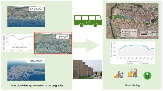
In this context, this paper presents an evaluation of the impact of the spatial resolution of point clouds for the estimation of street slopes, based on the analysis of point clouds acquired from different platforms (aerial and terrestrial). The results of the optimal point cloud density are applied to a problem of route optimization, searching for the most efficient route (the route with the lowest steep slopes). Both studies are performed through their application to the case study of the city of Ávila, selected because of it being a city that is representative of cities with varied orography.

2. Materials and Methods

2.1. LiDAR Point Cloud

Many European countries make spatial data freely available to users based on the INSPIRE (Infrastructure for Spatial Information in Europe) initiative [37]. However, some countries also count on public national entities that offer updated information of the territory. One example of this is the Instituto Geográfico Nacional (IGN) in Spain that offers a wide variety of free updated geoinformation based on INSPIRE through a geoportal [33]. Orthoimages and point clouds are the most demanded products. Their acquisition is part of the PNOA/PNOA LiDAR project with an updating period of 2 to 4 years [34].
For this research, LiDAR data with different densities from IGN were used. PNOA-LiDAR data are classified according to the date of acquisition, the first coverage data (2009–2015) with a density for the whole extension of 0.5 points/m2 and the second coverage data (2015-present) with a variable density between 0.5 and 4 points/m2, with some exceptions in which the density is higher. These are RGB point clouds classified in the ASPRS Classes. Specifically, for the study area described below, the available point clouds have a density of 0.5 points/m2 (first coverage) and 1 point/m2 (second coverage). Regarding the equipment, in both cases the data were captured with a Leica Laser Scanner, model ALS50 for the density of 0.5 points/m2 and model ALS80 for the density of 1 point/m2.
The main disadvantage of the free products is that they cover such large areas that the resolution is significantly reduced compared to data collection over smaller areas. There is a variety of LiDAR equipment available, both airborne and ground-based, which allows three-dimensional reconstruction of the environment with high resolution. In order to find out whether low-density point clouds allow an accurate topographic characterization, the methodology presented below was also carried out using data captured with mobile LiDAR equipment with a resolution of 38 points/m2. Specifically, the equipment used was Lynx Mobile Mapper M1 from Optech with a 360° field of view (FOV) in combination with an Applanix POS LV 520 positioning and navigation system that used Trimble GNSS receivers (Table 1) [38]. The resulting point cloud contains not only the X, Y, and Z position of each point but also the intensity value, time stamp of acquisition of the point, and return number. The data acquisition took place in February 2020 with a density of 38 points/m2.

2.2. Case of Study: Ávila (Spain)

Ávila is a Spanish city located in the center of the Iberian Peninsula (Figure 1a). It has an area of 230 km2 and 57,949 inhabitants at an altitude of 1128 m above sea level, being the city in Spain at the highest altitude [39]. This height implies that, in terms of climatology, Ávila has a climate with an average temperature that varies between −1 °C and 29 °C, with very cold winters and short, hot summers [40].
According to the size of the city, buses are the main form of public transport. The urban bus network is made up of a total of 6 lines that serve the main areas of the city (Figure 1b): the hospital, the university area, the national police school, and the main urbanization of the city (El Pinar). Within all the bus lines, there are two typologies depending on their route: (i) those that make a single closed route (circular routes) and (ii) those that make a one-way route different from the return route (lineal routes), using different buses for each of the journeys. The average number of stops for circular routes is 45 stops, while for each of the journeys on non-circular routes it is 27 stops. The average route length for non-circular routes is almost 8 km, while circular routes have average lengths of 14.40 km. In terms of slope, the maximum slope reached is 14.19% on route 2 (return), while the minimum slope reached is 7.20% on route 6 (return). The following table shows in detail the main characteristics for each route (Table 2). It can be seen that thanks to the different bus routes and the great variety of parameters such as length and different elevations, the city of Ávila is a good case study to analyze the effect of point cloud density in the determination of topography and the effect of topography in the consumption of electric buses.

2.3. Methodology

To assess the influence of point cloud density on the estimation of terrain slope, for each of the point clouds used, a three-step methodology was followed (Figure 2):
  • DEM generation: Using Global Mapper with the different point clouds, the digital elevation model based on the triangulated irregular network or TIN method was generated. In the case of the point clouds of IGN for processing, points with classification type: 0-Created, never classified; 1-Unclassified; 2-Ground; and 11-Road were used in order to have the most complete representation possible for the ground. The point cloud is classified semi-automatically by IGN [41]. In this process, some terrain points are not classified correctly, so unclassified points are considered to avoid loss of information.
  • Generation of the longitudinal profile of each route: Extraction of the longitudinal profile with the outline of each route on the DEM. Global Mapper software is used for this task.
  • Slope estimation and categorization: For each of the topographic profiles obtained, the slope was calculated in 10-m sections as the average value of the slopes of the paths in order to subsequently categorize the sections according to slopes for better analysis. The slope categorization criteria followed are summarized in the following table (Table 3).
Figure 2. Workflow followed for the evaluation of point cloud density in slope estimation.
Remotesensing 15 03325 g002

3. Results

Figure 3 shows one of the three DEMs resulting from the first step of the above methodology, obtained from a point cloud acquired by the IGN with 1 point/m2 spatial resolution.
DEM generation was performed in a computer with an Intel Xeon ES-609 processor with 64 GB of RAM and an 8 Gb NVDIA RTX 3060 graphics card. Table 4 shows the processing times and the size of the resulting DEMs for each point cloud density used.
From the DEMs, topographic profiles were obtained for each of the bus routes previously described. The following image (Figure 4) shows the resulting profiles for each bus route in the city of Ávila, showing the adequacy of the selection of the city through the large variety of changes in the elevations along the different routes.
Figure 5a shows the result of generating and superimposing the topographic profile for each of the point cloud densities. Visually, there are hardly any differences in the geometry, except in specific areas, as can be seen in Figure 5b.
Using the topographic profiles (Figure 4) and based on the categorization described in Section 2.3, the slopes on each route were calculated and classified for the different DEM densities. Figure 6, Figure 7 and Figure 8 show graphically, in relation to the total length, the percentage of positive slope (greater than 3%), negligible slope (between 3 and −3%), and negative slope (less than −3%) present in each route. With these results, it can be seen that there is no noticeable difference in the use of a low-density point cloud (1 point/m2) versus a high-density point cloud (38 points/m2) for the estimation of the slope of the terrain.
For all DEMs, the results show that most of the routes analyzed have negligible slopes. Route 6 has the largest route section with a negligible slope (81%), while route 1 has the shortest (59%). With regard to the sections with positive and negative slopes, the results are very similar, since these represent between 10 and 20% of the total length of the bus routes.

4. Discussion

A deeper analysis of the difference between the use of different point cloud densities for slope estimation was performed for each slope value obtained based on the difference between the highest density (used as reference) and the lower densities. The results obtained from this comparison (Figure 9 and Figure 10) show a different behavior of the point clouds according to the degree of the slope. For those parts of the route with a slope of more than 5%, the differences are practically negligible, as is the case for slopes of less than −5%, with an average difference in the estimation of 0.22% for a density of 0.5 points/m2 regarding the density calculated from the 38 points/m2 point cloud. For a density of 1 point/m2, the average difference is 0.20%. In the case of the less-steep slopes: for a density of 0.5 points/m2, the difference regarding the high-density DEM (38 points/m2) is 0.96%, while for a 1 point/m2 density it is 0.65%. The maximum difference values for both densities are found when the terrain has no slope. Specifically, in the case of the point cloud with 1 point/m2 resolution, the maximum differences with the 38 points/m2 reached are 2% (Line 2) and −1.5% (Line 5). For the case of the point cloud with a resolution of 0.5 points/m2, the maximum differences are 3.25% (Line 2) and −2.79% (Line 2).
These results lead to the conclusion that the use of low-density point clouds with a resolution of 1 point/m2 captured with LiDAR makes it possible to accurately characterize the orography with significant slopes, with errors in the determination of the plain terrain (slope below 2%), thus showing a good compromise between the accuracy obtained and the processing time required.

5. Application Case

The adequacy of the use of a low-density point cloud for the accurate characterization of the orography is shown in this section through its use for one of the main applications of this type of geomatic product in the field of urban mobility: the estimation of optimized routes for electric buses. Taking the DEM from a point cloud with a resolution of 1 point/m2 as a starting point in accordance with the results of the previous section, the design and evaluation of a route in the urban center of the city of Ávila are carried out. This route has to fulfill several requirements: (i) it has to cover strategic points of interest for both inhabitants and tourists; (ii) the length should be as short as possible; (iii) the slopes of the route should have the minimum possible gradient; (iv) the starting and end point of the route is the same: “Palacio de Congresos Lienzo Norte”.

5.1. Conditions of the Route

Among all the bus routes that currently operate in Ávila, there is not one that covers the historic center of the city. This is an area characterized by a significant difference in altitude within the city. This, together with its tourist potential, makes it an interesting route for urban transport in the city. In order to provide the user a better service, the design route should be circular and include a series of strategic points for tourism and user demand (Figure 11):
1.  
Palacio de Congresos “Lienzo Norte”.
2.  
Centro de recepción de Visitantes.
3.  
Subdelegación provincial de educación.
4.  
Delegación provincial de la Junta de Castilla y León.
5.  
Plaza de Salamanca.
6.  
Colegio Santa Teresa.
7.  
Iglesia de San Vicente/Catedral.
8.  
Plaza de Zurraquín (Ayuntamiento).
9.  
Palacio de Benavites (Parador de Turismo).
10.
Palacio de Polentinos/Iglesia Santa Teresa.
11.
Iglesia de San Esteban/Hornos Postmedievales.
12.
Puerta de la Muralla del Adaja/Tenerías/Acceso Muralla.
Figure 11. Locations of the strategic points for the design of the new route.
Remotesensing 15 03325 g011

5.2. Possible Routes

Two routes have been designed to fit the established criteria using QGIS network analysis tools to obtain the routes, leaving all the mandatory crossing points except for the two possible options for Centro de recepción de Visitantes: option 1 with a total length of 4639 km and option 2 with a total length of 4575 km (Figure 12 and Figure 13).
Although both paths are similar (Figure 14), the main difference is the slope between 460 m and 2240 m from the start of the route. While option 1 presents a very steep slope between the two positions with an average value of 4.43%, option 2 avoids this stretch with a more progressive slope with an average value of 2.63%. As for the maximum value in this part of the route, option 1 reaches a value of 11.19%, while option 2 reaches a value of half (5.54%).
According to the categorization criteria previously described, it can be seen that option 2 has a greater length of its route without slopes (Figure 15). Only 7.42% of the total route has a slope of more than 5% compared to 14.21% in option 1.
From all the orography data provided in the detailed analysis of the two resulting options, it can be concluded that, of the two options analyzed, option 2 is the most suitable for the implementation of electric buses, as it has a lower percentage of sections with steep slopes.

5.3. Economic and Environmental Analysis Based on Fuel Consumption Estimation

Considering that the designed route (4575 m) would be repeated 30 times a day during working days (Monday to Friday) and 40 times on weekends (Saturdays and Sundays) due to a higher tourist demand, the annual distance is 54,867 Km. The savings in emissions and fuel costs of the current bus models used (diesel buses) are analyzed compared to an electric bus model. Bus consumption depends on multiple factors (such as driving patterns, slope, or load factor) and requires real data acquisitions [42]. Due to the unfeasibility of acquiring real-time operational data, the proposed economic and environmental analysis assumes consumption parameters based on the scientific article by Giraldo et al. [43]. The following table (Table 5) contains all the parameters considered for the analysis.
Fuel costs are calculated for each type of bus. Table 6 shows the cost associated with each type of technology. The electric bus supposes an 18.10% reduction in operational cost related to the diesel bus energy consumption.
From an environmental point of view, Table 7 shows the emissions produced by the two bus models. The electric bus is the model with the lowest impact on the environment due to emissions. In terms of CO2, considering the Kg of CO2 equivalent per KWh of produced emissions of Spanish electrical mix production for the year 2022, the use of an electric bus reduces its emissions by 32.59% of those of the diesel model. Considering renewable electricity production, these emissions could be reduced entirely.
The obtained results are based on estimated consumption, so factors such as slope, driving style, and the number of passengers are considered in their effect on consumption in an approximate manner, as they directly affect consumption regardless of the type of bus. However, for the case of the e-bus, the advantages of regenerative braking or the use of supercapacitors [44] in reducing consumption in this type of bus are not considered. Therefore, applying these considerations to the analysis would result in even better results than those obtained.
In terms of slope routes, it is worth mentioning the potential reduction in waiting times due to the greater acceleration of e-buses compared to diesel buses, thanks to their higher torque.

6. Conclusions

The integration of electric vehicles as a means of transport is one of the main challenges of society towards the reduction in CO2 emissions. While it is true that the key point lies in technology, there are a number of factors that contribute to its successful implementation.
This scientific article analyzes one of the main issues that most influences the performance of electric technologies when it comes to urban mobility: orography. From a geospatial perspective, this work analyzes the influence of the density of a point cloud in the estimation of a slope using the urban bus routes of the city of Ávila as a case study. Although higher-resolution products provide better results, their computational cost is considerably higher (39 and 17 times more time compared to the lower resolution products of 0.5 and 1 point/m2, respectively). Thus, this research has shown that, in the case of slope estimation, a low-density point cloud (1 point/m2) can accurately characterize the terrain (maximum error of 2%) without increasing processing times or the weight of the final product (39 times lower storage capacity needed).
Following the results of the research, the second part of the article shows a real case of application in urban mobility: the design of a bus route. Taking as a starting point a set of conditions and the DEM derived from a low-density point cloud (1 point/m2), two possible routes are obtained. For both routes, the slopes along the entire route are analyzed. In option 1, which covers a total of 4639 kms, 14% of the total route has a slope of more than 5%, while option 2, which covers a total of 4575 km, halves the percentage of the route with a slope of more than 5%. For this reason, based on the most suitable route (option 2) for electrification, a detailed study is made of the economic and environmental savings implicit in comparison with current urban buses. The results show that the implementation of electric buses vs. diesel buses would reduce greenhouse gas emissions in the city to a large extent (17.27 T CO2/bus and 290.8 kg NOx/bus). On this basis, the use of electric vehicles is indispensable for a sustainable and environmentally friendly future.

Author Contributions

Conceptualization, M.S.-A. and S.L.; methodology, M.S.-A.; software, J.A.M.-J.; validation, M.S.-A., J.A.M.-J. and E.G.-G.; formal analysis, M.S.-A.; writing—original draft preparation, M.S.-A.; writing—review and editing, S.L., J.A.M.-J. and E.G.-G.; funding acquisition, S.L. All authors have read and agreed to the published version of the manuscript.

Funding

This research has been funded by several sources: IBERDROLA SAU. through the collaboration contract with Universidad de Salamanca with reference number 2020/00071/001, the European Union through Fondo Social Europeo (EDU/601/2020), the European Union’s Horizon 2020 research and innovation programme under grant agreement No 101021714 (Project LAW-GAME) and NextGenerationEU programme under grant reference CPP2021-008863 (ROAD-EYE project). Views and opinions expressed are however those of the authors only and do not necessarily reflect those of the European Union or the European Research Executive Agency. Neither the European Union nor the European Research Executive Agency can be held responsible for them.

Data Availability Statement

Not applicable.

Acknowledgments

The authors express their gratitude to Ayuntamiento de Ávila for their support in this article.

Conflicts of Interest

The authors declare no conflict of interest. The funders had no role in the design of the study; in the collection, analyses, or interpretation of data; in the writing of the manuscript; or in the decision to publish the results.

References

  1. United Nations Environment Programme. Cities and Climate Change. Available online: https://www.unep.org/explore-topics/resource-efficiency/what-we-do/cities/cities-and-climate-change (accessed on 18 March 2023).
  2. Steinberg, D.; Bielen, D.; Eichman, J.; Eurek, K.; Logan, J.; Mai, T.; Mcmillan, C.; Parker, A.; Vimmerstedt, L.; Wilson, E. Electrification & Decarbonization: Exploring U.S. Energy Use and Greenhouse Gas Emissions in Scenarios with Widespread Electrification and Power Sector Decarbonization; National Renewable Energy Lab. (NREL): Golden, CO, USA, 2017.
  3. International Energy Agency. Global EV Outlook 2021. Accelerating Ambitions Despite the Pandemic; International Energy Agency: Paris, France, 2021.
  4. International Energy Agency. Electric Vehicles. 2022. Available online: https://www.iea.org/reports/electric-vehicles (accessed on 18 March 2023).
  5. IES-Synergy. Electric Buses: Where Are We? 2021. Available online: https://www.ies-synergy.com/en/electric-buses-where-are-we/ (accessed on 18 March 2023).
  6. Wired. How Shenzhen Turned All Its 16,000 Buses Fully Electric. 2020. Available online: https://www.wired.co.uk/article/shenzhen-electric-buses-public-transport (accessed on 18 March 2023).
  7. Roderick, W.; Watson, C.; Firth, D.; Sutherland, C.; Sadouni, I.; Goff, K.; Bickle, E.; Dixon, N.; Samuels, D.; Saville, C.; et al. C40 Green and Healthy Streets Declaration; Annual City Progress Report; C40 Cities: London, UK, 2022. [Google Scholar]
  8. ZeEUS. ZeEUS-Zero Emission Urban Bus System. 2014. Available online: https://zeeus.eu/ (accessed on 18 March 2023).
  9. Transport & Environment. Cities Are Buying More Electric Buses, but an EU Deadline Is Needed. 2022. Available online: https://www.transportenvironment.org/discover/cities-are-buying-more-electric-buses-but-an-eu-deadline-is-needed/ (accessed on 18 March 2023).
  10. Sustainable Bus. The Netherlands Have More than 1000 Electric Buses in Operation. 2020. Available online: https://www.sustainable-bus.com/news/the-netherlands-have-more-than-1000-electric-buses-in-operation/ (accessed on 18 March 2023).
  11. Grigorieva, O.; Nikulshin, A. Electric Buses on the Streets of Moscow: Experience, Problems, Prospects. Transp. Res. Procedia 2022, 63, 670–675. [Google Scholar] [CrossRef]
  12. Aldenius, M.; Mullen, C.; Pettersson-Löfstedt, F. Electric Buses in England and Sweden—Overcoming Barriers to Introduction. Transp. Res. Part D Transp. Environ. 2022, 104, 103204. [Google Scholar] [CrossRef]
  13. Verbrugge, B.; Hasan, M.M.; Rasool, H.; Geury, T.; El Baghdadi, M.; Hegazy, O. Smart Integration of Electric Buses in Cities: A Technological Review. Sustainability 2021, 13, 12189. [Google Scholar] [CrossRef]
  14. Ayetor, G.K.; Mbonigaba, I.; Sunnu, A.K.; Nyantekyi-Kwakye, B. Impact of Replacing ICE Bus Fleet with Electric Bus Fleet in Africa: A Lifetime Assessment. Energy 2021, 221, 119852. [Google Scholar] [CrossRef]
  15. Basma, H.; Haddad, M.; Mansour, C.; Nemer, M.; Stabat, P. Evaluation of the Techno-Economic Performance of Battery Electric Buses: Case Study of a Bus Line in Paris. Res. Transp. Econ. 2022, 95, 101207. [Google Scholar] [CrossRef]
  16. Lopez de Briñas Gorosabel, O.; Xylia, M.; Silveira, S. A Framework for the Assessment of Electric Bus Charging Station Construction: A Case Study for Stockholm’s Inner City. Sustain. Cities Soc. 2022, 78, 103610. [Google Scholar] [CrossRef]
  17. Perrotta, D.; Macedo, J.L.; Rossetti, R.J.F.; Sousa, J.F.d.; Kokkinogenis, Z.; Ribeiro, B.; Afonso, J.L. Route Planning for Electric Buses: A Case Study in Oporto. Procedia-Soc. Behav. Sci. 2014, 111, 1004–1014. [Google Scholar] [CrossRef] [Green Version]
  18. Papa, G.; Santo Zarnik, M.; Vukašinović, V. Electric-Bus Routes in Hilly Urban Areas: Overview and Challenges. Renew. Sustain. Energy Rev. 2022, 165, 112555. [Google Scholar] [CrossRef]
  19. Liu, K.; Yamamoto, T.; Morikawa, T. Impact of Road Gradient on Energy Consumption of Electric Vehicles. Transp. Res. Part D Transp. Environ. 2017, 54, 74–81. [Google Scholar] [CrossRef]
  20. Wang, J.; Besselink, I.; Nijmeijer, H. Battery Electric Vehicle Energy Consumption Prediction for a Trip Based on Route Information. Proc. Inst. Mech. Eng. Part D J. Automob. Eng. 2018, 232, 1528–1542. [Google Scholar] [CrossRef] [Green Version]
  21. Sagaama, I.; Kchiche, A.; Trojet, W.; Kamoun, F. Impact of Road Gradient on Electric Vehicle Energy Consumption in Real-World Driving. In Advances in Intelligent Systems and Computing; Springer: Cham, Switzerland, 2020; Volume 1151, pp. 393–404. [Google Scholar]
  22. Bhushan, S.; Shean, D.; Alexandrov, O.; Henderson, S. Automated Digital Elevation Model (DEM) Generation from very-High-Resolution Planet SkySat Triplet Stereo and Video Imagery. ISPRS J. Photogramm. Remote Sens. 2021, 173, 151–165. [Google Scholar] [CrossRef]
  23. Shaker, A.; Yan, W.Y.; LaRocque, P.E. Automatic Land-Water Classification using Multispectral Airborne LiDAR Data for Near-Shore and River Environments. ISPRS J. Photogramm. Remote Sens. 2019, 152, 94–108. [Google Scholar] [CrossRef]
  24. Tijerín-Triviño, J.; Moreno-Fernández, D.; Zavala, M.A.; Astigarraga, J.; García, M. Identifying Forest Structural Types Along an Aridity Gradient in Peninsular Spain: Integrating Low-Density LiDAR, Forest Inventory, and Aridity Index. Remote Sens. 2022, 14, 235. [Google Scholar] [CrossRef]
  25. Fernández-Arango, D.; Varela-García, F.A.; González-Aguilera, D.; Lagüela-López, S. Automatic Generation of Urban Road 3D Models for Pedestrian Studies from LiDAR Data. Remote Sens. 2022, 14, 1102. [Google Scholar] [CrossRef]
  26. Martín-Jiménez, J.; Del Pozo, S.; Sánchez-Aparicio, M.; Lagüela, S. Multi-Scale Roof Characterization from LiDAR Data and Aerial Orthoimagery: Automatic Computation of Building Photovoltaic Capacity. Autom. Constr. 2020, 109, 102965. [Google Scholar] [CrossRef]
  27. Sharma, M.; Garg, R.D.; Badenko, V.; Fedotov, A.; Min, L.; Yao, A. Potential of Airborne LiDAR Data for Terrain Parameters Extraction. Quat. Int. 2021, 575–576, 317–327. [Google Scholar] [CrossRef]
  28. Urbazaev, M.; Hess, L.L.; Hancock, S.; Sato, L.Y.; Ometto, J.P.; Thiel, C.; Dubois, C.; Heckel, K.; Urban, M.; Adam, M.; et al. Assessment of Terrain Elevation Estimates from ICESat-2 and GEDI Spaceborne LiDAR Missions Across Different Land Cover and Forest Types. Sci. Remote Sens. 2022, 6, 100067. [Google Scholar] [CrossRef]
  29. Ågren, A.M.; Larson, J.; Paul, S.S.; Laudon, H.; Lidberg, W. Use of Multiple LIDAR-Derived Digital Terrain Indices and Machine Learning for High-Resolution National-Scale Soil Moisture Mapping of the Swedish Forest Landscape. Geoderma 2021, 404, 115280. [Google Scholar] [CrossRef]
  30. Rocha, J.; Duarte, A.; Fabres, S.; Quintela, A.; Serpa, D. Influence of DEM Resolution on the Hydrological Responses of a Terraced Catchment: An Exploratory Modelling Approach. Remote Sens. 2023, 15, 169. [Google Scholar] [CrossRef]
  31. Tondo, M.; Mulas, M.; Ciccarese, G.; Marcato, G.; Bossi, G.; Tonidandel, D.; Mair, V.; Corsini, A. Detecting Recent Dynamics in Large-Scale Landslides Via the Digital Image Correlation of Airborne Optic and LiDAR Datasets: Test Sites in South Tyrol (Italy). Remote Sens. 2023, 15, 2971. [Google Scholar] [CrossRef]
  32. Fernández-Alonso, J.M.; Llorens, R.; Sobrino, J.A.; Ruiz-González, A.D.; Alvarez-González, J.G.; Vega, J.A.; Fernández, C. Exploring the Potential of Lidar and Sentinel-2 Data to Model the Post-Fire Structural Characteristics of Gorse Shrublands in NW Spain. Remote Sens. 2022, 14, 6063. [Google Scholar] [CrossRef]
  33. Instituto Geográfico Nacional. Centro de Descargas del CNIG (IGN). Available online: https://centrodedescargas.cnig.es/CentroDescargas/index.jsp (accessed on 3 June 2020).
  34. Arozarena, A.; Villa, G.; Valcárcel, N. The National Aerial Ortophoto Program in Spain (PNOA). In Proceedings of the International Cartographic Conference, La Coruña, Spain, 9–16 July 2005. [Google Scholar]
  35. Peng, C.; Hsu, C.; Wang, W. Cost Effective Mobile Mapping System for Color Point Cloud Reconstruction. Sensors 2020, 20, 6536. [Google Scholar] [CrossRef]
  36. Qiu, Z.; Martínez-Sánchez, J.; Brea, V.M.; López, P.; Arias, P. Low-Cost Mobile Mapping System Solution for Traffic Sign Segmentation using Azure Kinect. Int. J. Appl. Earth Obs. Geoinf. 2022, 112, 102895. [Google Scholar] [CrossRef]
  37. Bartha, G.; Kocsis, S. Standardization of Geographic Data: The European INSPIRE Directive. Eur. J. Geogr. 2011, 2, 79–89. [Google Scholar]
  38. Puente, I.; González-Jorge, H.; Riveiro, B.; Arias, P. Accuracy Verification of the Lynx Mobile Mapper System. Opt. Laser Technol. 2013, 45, 578–586. [Google Scholar] [CrossRef]
  39. Diputación de Ávila. Ávila, Municipio de La Provincia de Ávila. 2019. Available online: https://www.diputacionavila.es/la-provincia/nuestros-pueblos/avila.html (accessed on 18 March 2023).
  40. Weather Spark. El Clima En Ávila, El Tiempo Por Mes, Temperatura Promedio (España). 2023. Available online: https://es.weatherspark.com/y/35538/Clima-promedio-en-%C3%81vila-Espa%C3%B1a-durante-todo-el-a%C3%B1o (accessed on 18 March 2023).
  41. Centro Nacional de Información Geográfica. PNOA LiDAR: Procesamiento de Datos. 2023. Available online: https://pnoa.ign.es/pnoa-lidar/procesamiento-de-los-datos (accessed on 12 June 2023).
  42. Carrese, S.; Gemma, A.; La Spada, S. Impacts of Driving Behaviours, Slope and Vehicle Load Factor on Bus Fuel Consumption and Emissions: A Real Case Study in the City of Rome. Procedia-Soc. Behav. Sci. 2013, 87, 211–221. [Google Scholar] [CrossRef]
  43. Giraldo, M.; Huertas, J.I. Real Emissions, Driving Patterns and Fuel Consumption of in-use Diesel Buses Operating at High Altitude. Transp. Res. Part D Transp. Environ. 2019, 77, 21–36. [Google Scholar] [CrossRef]
  44. Naseri, F.; Karimi, S.; Farjah, E.; Schaltz, E. Supercapacitor Management System: A Comprehensive Review of Modeling, Estimation, Balancing, and Protection Techniques. Renew. Sustain. Energy Rev. 2022, 155, 111913. [Google Scholar] [CrossRef]
Figure 1. Location of Ávila city: (a) urban extension; (b) bus routes in 2020.
Remotesensing 15 03325 g001
Figure 3. Three-dimensional view of study bus lines on the resulting DEM (1 point/m2).
Remotesensing 15 03325 g003
Figure 4. Topographical profiles obtained from the DEM (point cloud with 1 point/m2) for each bus route analyzed.
Remotesensing 15 03325 g004
Figure 5. Superimposition of the topographic profiles of bus line 3 for the three densities analyzed: (a) resulting topographic profile of the area with differences marked with a red rectangle; (b) detail of the area of the topographic profile with significant differences.
Remotesensing 15 03325 g005
Figure 6. Positive slope (>3%) with respect to the total length for each of the bus lines for the different point densities analyzed.
Remotesensing 15 03325 g006
Figure 7. Negligible slope (between 3% and −3%) with respect to the total length for each bus line for the different point densities analyzed.
Remotesensing 15 03325 g007
Figure 8. Negative slope (<−3%) with respect to the total length for each bus line for the different point densities analyzed.
Remotesensing 15 03325 g008
Figure 9. Differences in estimated slopes of bus routes: 38 points/m2 vs. 1 point/m2.
Remotesensing 15 03325 g009
Figure 10. Differences in estimated slopes of bus routes: 38 points/m2 vs. 0.5 points/m2.
Remotesensing 15 03325 g010
Figure 12. Possible route, option 1: (a) bus trajectory with strategic points; (b) topographical profiles obtained from the DEM (point cloud with 1 point/m2).
Remotesensing 15 03325 g012
Figure 13. Possible route, option 2: (a) bus trajectory with strategic points; (b) topographical profiles obtained from the DEM (point cloud with 1 point/m2).
Remotesensing 15 03325 g013
Figure 14. Topographical profiles obtained from the DEM (point cloud with 1 point/m2): option 1 vs. option 2.
Remotesensing 15 03325 g014
Figure 15. Slope classification (%) in relation to the total length (%): option 1 vs. option 2.
Remotesensing 15 03325 g015
Table 1. Manufacturer specifications for the Lynx Mobile Mapper [38].
Number of LiDAR Sensors1–2
Camera supportUp to 4 × 5 Mpx cameras
Maximum range200 m, 20%
Range precision8 mm, 1σ
Absolute accuracy±5 cm (1σ)
Laser measurement rate75–500 kHz programmable
Measurement per laser pulseUp to 4 simultaneous
Scan frequency80–200 Hz programmable
Scanner field of view360° without obscurations
Number of LiDAR sensors1–2
Table 2. Main characteristics of Ávila’s bus routes.
RouteNameNumber of StopsTypeDirectionLength (Km)
1Escuela de Policía-San Nicolas21Lineal RouteOutward journey5.675
25Return7.464
2Centro Universitario-Hospital provincial30Lineal RouteOutward journey7.809
19Return4.921
3Circular46Circular route-14.282
4Escuela de Policía-El Pinar24Lineal RouteOutward journey7.733
27Return8.705
5Circular45Circular route-14.509
6Escuela de Policía-Igualdad33Lineal RouteOutward journey9.438
35Return11.133
Table 3. Slope categories used as classification criteria.
CategorySlope
Very steep positive slope>11%
Steep positive slope11–9%
Slightly steep positive slope9–7%
Medium positive slope7–5%
Gentle positive slope5–3%
Low positive slope3–1%
Flat area (no gradient)1–(−1)%
Gentle negative slope(−1)–(−3)%
Slight negative slope(−3)–(−5)%
Medium negative slope(−5)–(−7)%
Steep negative slope(−7)–(−9)%
Very steep negative slope<(−9)%
Table 4. Main characteristics of interest in data processing.
FeaturePoint Cloud Density (Points/m2)
0.5 138
Size (GB)0.7472.1279.54
Processing time (minutes)14.532.3581.4
Table 5. Parameters used for the evaluation of operational costs: electric model vs. diesel model.
Electric ModelDiesel Model
Consumption2.30 (KWh/Km)0.41 (l/Km)
Price0.204 (EUR/KWh)1.40 (EUR/l)
Em. CO20.368 (Kg/Km)0.9658 (Kg/Km)
Em. CO0.0 (Kg/Km)0.0414 (Kg/Km)
Em. NOx0.0 (Kg/Km)0.0053 (Kg/Km)
Table 6. Price of urban buses and savings: electric model vs. diesel model.
Electric ModelDiesel ModelSavings
Cost25,794.23 (EUR)31,493.84 (EUR)5699.62 (EUR)
Table 7. Main emissions for an electric model vs. diesel model of an urban bus.
EmissionsElectric ModelDiesel Model
CO235.72 (T) 52.99 (T)
CO0.0 (Kg)2.27 (T)
NOx0.0 (Kg)290.8 (Kg)
Disclaimer/Publisher’s Note: The statements, opinions and data contained in all publications are solely those of the individual author(s) and contributor(s) and not of MDPI and/or the editor(s). MDPI and/or the editor(s) disclaim responsibility for any injury to people or property resulting from any ideas, methods, instructions or products referred to in the content.

