Technical Note

Quantifying Multifrequency Ocean Altimeter Wind Speed Error Due to Sea Surface Temperature and Resulting Impacts on Satellite Sea Level Measurements

by
Ngan Tran
1,*,
Douglas Vandemark
2,
François Bignalet-Cazalet
3 and
Gérald Dibarboure
3
1
Collecte Localisation Satellites, 11 Rue Hermès, 31520 Ramonville Saint-Agne, France
2
Ocean Process Analysis Laboratory, Institute for the Study of Earth, Oceans, and Space, University of New Hampshire, Durham, NH 03824, USA
3
Centre National d’Etudes Spatiales, 18 Avenue Edouard Belin, CEDEX 09, 31401 Toulouse, France
*
Author to whom correspondence should be addressed.
Remote Sens. 2023, 15(13), 3235; https://doi.org/10.3390/rs15133235
Submission received: 8 May 2023 / Revised: 30 May 2023 / Accepted: 20 June 2023 / Published: 22 June 2023
(This article belongs to the Special Issue Advances in Satellite Altimetry)

Abstract

:
Surface wind speed measurements from a satellite radar altimeter are used to adjust altimeter sea level measurements via sea state bias range correction. We focus here on previously neglected ocean radar backscatter and subsequent wind speed variations due to sea surface temperature (SST) change that may impact these sea level estimates. The expected error depends on the radar operating frequency and may be significant at the Ka band (36 GHz) frequency chosen for the new Surface Water and Ocean Topography (SWOT) satellite launched in December 2022. SWOT is expected to revolutionize oceanography by providing wide-swath Ka band observations and enhanced spatial resolution compared to conventional Ku band (14 GHz) altimetry. The change to the Ka band suggests a reconsideration of SST impact on wind and sea level estimates, and we investigate this in advance of SWOT using existing long-term Ku and Ka band satellite altimeter datasets. This study finds errors up to 1.5 m/s in wind speed estimation and 1.0 cm in sea level for AltiKa altimeter data. Future SWOT data analyses may require consideration of this dependence prior to using its radar backscatter data in its sea level estimation.

1. Introduction

Sea level (SL) and sea surface temperature (SST) are two essential climate variables (ECVs) [1,2] monitored by the Global Climate Observing System (GCOS) since their increases are two visible consequences of global warming. Their inherent relationship is complicated, but it is intensely analyzed to understand how SL rise, ocean warming, and sea surface topography interact and affect our planet as climate varies [3,4,5,6]. SL is a particularly sensitive index of climate change since it integrates the impacts of both ocean warming through the thermal expansion process and ice mass loss from glaciers and ice sheets [7,8,9]. Over the past 30 years, SL has been routinely measured from space by conventional Ku band altimetry missions. The series started with the TOPEX/Poseidon satellite in 1992, then was followed successively by Jason-1, -2, and -3 missions with regular global coverage, frequent revisits at 10-day intervals, and the same ground track as TOPEX/Poseidon. These missions have provided the most accurate long-term global mean sea level (GMSL) time series from 1993 to the present. The latest release, produced by the French space agency (CNES) and distributed on the AVISO+ website, indicates a GMSL rise of 3.3 mm/yr (from January 1993 to December 2021) with an unprecedented uncertainty estimate of ±0.3 mm/yr at the 90% confidence level [10]. This very good result has been reached thanks to accuracy improvement efforts continuously made in all the different aspects of the altimetry system and to data reprocessing that takes advantage these updated versions.
However, the recommended GMSL trend uncertainty requirement from both GCOS and the Intergovernmental Panel on Climate Change (IPCC) has still not been met: 0.3 mm/yr over 10-year periods [11]. Among the major factors leading to GMSL measurement noise levels of about ±0.5 mm/yr over 10-year periods, correlated errors at short timescales (annual and below) have been identified [10]. This calls for a better identification/understanding/characterization/quantification of these errors and/or uncertainties that may come from mixed origins that include altimeter noise, radiometer noise, geophysical correction uncertainties, modelling errors, and perhaps the currently more problematic geophysical signals, which, at first, were not considered or assumed to be negligible when focusing on bigger ones. The net result is in limiting both GMSL error budget assessment and GMSL rise uncertainty budget description. Being able to pinpoint the exact origins of the GMSL errors or uncertainties at short timescales and to identify the various improvements that could be made in the current altimetry observing system will help to meet the scientific demand for improving GMSL accuracy, stability, and the description of its uncertainty budget.
Among the potential errors affecting GMSL estimation, two are the accuracy and the long-term stability of the radar altimeter backscatter coefficient (s0). The latter is retrieved from the altimeter waveforms and is related to the power of the surface-reflected radar signal. Errors in its values will propagate successively through wind speed (U10) and sea state bias (SSB) estimations, finally impacting the SL records. Ablain et al. [12] reported that small 0.2 dB TOPEX s0 anomalies that lie within the instrumental stability requirements alter the GMSL trend by nearly 0.1 mm/yr over a 20-year satellite measurement period. This level of impact is significant given the GMSL stability goals. Ablain et al. [12] also highlighted that such features strongly affect interannual GMSL variations, with associated errors reaching 2 mm. Note that to reach 0.1 mm/yr stability in GMSL [13], it is necessary to have 0.01 dB/yr stability on s0 [14]. The usual requirement for s0 stability of 0.1 dB/yr seems to have been set too large and looks incompatible with the agreed-upon GMSL requirement.
Amongst the various attempts to reduce the error/uncertainty in the altimeter data record, SST’s direct impact on ocean s0 data has, thus far, been neglected because of its weak impact on Ku band measurements: at most, ~3% over the full interval of SST values [15]. However, this aspect may warrant a revisit since this expected error depends on the radar operating frequency and the large regional SST variations. Indeed, Vandemark et al. [15] pointed out a 14% variation in s0 in the Ka band linked to this SST effect on the flat surface reflectivity for seawater. This error looks significant in the Ka band and this is the operating frequency (36 GHz) for the new Surface Water and Ocean Topography (SWOT) satellite launched in December 2022. This mission opens a new era for satellite altimetry with the first-time provision of wide-swath observations.
The move towards the Ka band was dictated by the expressed scientific need for finer-scale observations of the mesoscale variability to a degree that allows a proper description of the oceanic eddy field and the interactions of this field with the mean field (i.e., at spatial resolutions of 15 km and larger). Such a constraint concerning the spatial and temporal resolution of a MSL measuring system also addresses requirements dealing with the sampling of the coastal dynamical features or the observation of continental waters. The SARAL (Satellite with ARgos and ALtiKa) mission launched on 25 February 2013 carries the first Ka band altimeter. Benefits/innovations related to the use of this microwave frequency have clearly emerged [16,17]. This opened the path for the SWOT mission designed to fulfill all requested requirements.
The questions that arise in this context for the altimetry community are whether this SST effect can still be ignored or not, and to what extent SST change directly influences SL rise through its computation and not indirectly through the thermal expansion mechanism. Moreover, in this context—where wind retrieval over oceans is well mastered from altimetry and scatterometry satellite systems and we are continuously seeking for higher data accuracy—errors and uncertainties coming from secondary factors not accounted for have been more largely quantified in recent years, and it is often shown that improved U10 accuracy may be achieved by considering them [15,18,19,20]. Thus, it seems crucial to more accurately characterize U10 and SL errors linked to SST to determine to what extent each mission is impacted by this potential effect and to provide recommendations to improve altimeter system components and reduce their uncertainties.
This paper aims to reconsider the SST impact on altimeter wind and sea level estimates. We investigate this in advance of SWOT using existing long-term Ku and Ka band altimeter datasets. This analysis goes one step further from the path initiated by Vandemark et al. [15] study. The latter analyzed the impact of SST on U10 based on a one-dimensional wind speed model; here, we work with two-dimensional models—the function of s0 and significant wave height (SWH)—used to generate the official GDR-F version of altimeter products to report impacts on records available to all. This issue may become more important as altimeter records are extended in the future and the effects of ocean warming become larger.
This paper is structured as follows. Section 2 and Section 3 describe the different datasets and provide an overview of Vandemark et al. [15] approach used to correct s0 for SST dependency, respectively. Section 4 provides an error assessment of both U10 and SL estimations. Finally, conclusions and outlooks are presented in Section 5.

2. Data Sources

Nadir-looking altimeters were first developed to measure SL, but the shape and size of the return signal, the waveform, contain a lot more information about the ocean surface such as SWH and s0, which can be used afterwards to infer the ocean surface wind speed. The latter is commonly defined as the value at a height of 10 m above the mean sea surface, U10. Although altimeters do not provide wind direction (like scatterometers), their s0 and subsequent wind data have been used for many applications, including the provision of point-to-point SSB range correction for accurate SL records, the validation of numerical weather prediction models [21,22], wind climatology and the investigation of long-term trends in oceanographic wind speed [23,24,25], rain effect investigations on altimetric data [26,27,28], ocean wave period estimation [29,30,31], and other direct uses of s0 data [32,33,34,35]. At the present time, the inversion model functions of altimeter U10 are purely empirical, and a variety of different relationships have historically been developed. Some directly translate s0 to U10 by using empirical functions that are calibrated with in situ buoys and/or model winds [21,36,37,38]. Refined models introduce a sea state dependence by including altimeter-measured SWH as a secondary parameter and proxy for the long-wave tilting of capillary waves. The latter are often developed using collocations between altimeter and scatterometer datasets [39,40,41].
As microwaves are scattered by wave facets larger than about 3 times the incident radar wavelength (~2.2 cm for the Ku band and ~0.8 cm for Ka), the Ka band s0 is more sensitive to small-scale waves, including shorter gravity–capillary waves that are more responsive to wind. Thus, the Ka band s0 exhibits a stronger wind speed dependence than that of the Ku band. This leads to known differences in the relationship between s0 and U10, particularly at moderate-to-high wind speeds when one compares Ka and Ku band data [32]. For low wind speeds, longer gravity waves contribute significantly to the total surface roughness, and backscatter differences between the Ka and Ku bands are less apparent. These observations dictate the development of frequency-specific U10 retrieval algorithms. There are other secondary air–sea interaction factors that may affect the measurement of s0 and, thus, the accuracy of U10 retrieval, but they are currently neglected.
As stated earlier, the main purpose of altimetric U10 is to describe the SSB range correction to obtain accurate SL data. SSB correction ranges from 3 to 30 cm in magnitude and it accounts for range errors from three sources: an electromagnetic bias, a skewness bias, and a term that combines contributions related to the instrument design, the signal processing, and the SL computation itself. Because the theoretical modeling and prediction of SSB remain outstanding challenges, operational SSB models are estimated empirically for each sensor and are frequency-dependent [42,43,44,45,46]. Uncertainties in any of the input estimates (SWH, U10, or possible wave parameters) used to determine this relation can propagate into the SSB model and are transferred to the SL record.
For this study, we used 1 Hz altimeter measurements extracted from two datasets compiled over the period of the year 2015; the distance between two successive 1 Hz samples is ~7 km. The datasets are both based on level-2 GDR (Geophysical Data Records) products made freely available by CNES and AVISO (Archiving, Validation, and Interpretation of Satellite Oceanographic data). The Ka band data come from the AltiKa altimeter in its latest processing version (GDR-F) [47], while the Ku band ones are from the Jason-2 altimeter launched on 20 June 2008, also in its latest processing version available at the time of this study (version D) [48]. s0, altimeter U10, and SSB data are provided in these GDRs. U10 estimations are based on 2D models: Collard’s [40] model is used for Jason-2 data, while Tran et al. [41] model is used for AltiKa data. SSB models in their 2D version (based on SWH and U10) are also used as indicated in each altimeter product handbook. Coincident U10 estimations from analyses by the ECMWF Integrated Forecasting System (IFS) (6 hourly, 0.5° spatial resolution) are also provided in these products; the interpolation at the altimeter time and position is performed in the product generation chain. For the altimeter quality control, we used the CLS screening process from cal/val activities to discard all questionable measurements including sea-ice-contaminated data.
Concerning ancillary SST data, they come from NOAA optimal interpolated sea surface temperature daily products (OISST version 2, also known as Reynolds’ SST) based on AVHRR sensors and in situ observations [49]. They are provided on a global regular 0.25° (~30 km) grid. For this study, the OISST data were interpolated in space and time to coincide with each altimeter measurement and added in each dataset. Note that SST estimations from an hourly L4 product distributed through the Copernicus Marine Service—the OSTIA (Operational Sea Surface Temperature and Ice Analysis) SST product produced by the U.K. Met Office [50]—were also used over a 10-month period (availability started from 24 February 2015 only). The result differences were small, did not significantly change our conclusions, and are not reported hereafter. The main SST variation (between −2 and 32 °C) is observed with respect to latitude; then, the annual variation cycle can reach ~10 °C locally and the diurnal variation related to the local measurement time is only up to ~3 °C. At the first order, it is thus the latitudinal variation in SST that will be discussed in the following global SST impact evaluations, and OISST data are relevant for that purpose. The altimeter U10 bias against both averaged SST and ECMWF wind speed levels is examined in Figure 1. Wind speed differences between the altimeter and ECMWF were binned into 1° in SST and 0.5 m/s in ECMWF wind speed boxes; then, the mean wind speed biases were calculated as a function of the wind speed and SST. The results are displayed separately for the Ka and Ku band altimeters. They show evidence of a systematic SST-dependent error in the altimeter U10 estimations over the common values between 2 and 18 m/s. The bias patterns are similar in panels (a) and (b). Altimeter estimations are globally larger over cold waters than values indicated by the model, while they are lower in very-warm-SST and high-wind-speed conditions. The SST-related error in the Ka band is greater than in the Ku band. The results suggest that Ku vs. Ka band biases (i.e., main features) do not depend on the model used for wind retrieval, but appear likely to come from the same geophysical phenomenon, an SST dependence on s0 that is frequency-dependent. These results confirm the observations previously reported in Vandemark et al. [15] study, based on a 1D wind model, for which they proposed a correction that is described in the next section.
Note that this study focuses strictly on the frequency-dependent dielectric change with the temperature of sea water itself: the so-called flat surface radar reflectivity. There exists another SST–wind coupling related to a local/dynamical phenomenon occurring across SST gradients. Indeed, wind accelerates over warmer water masses and decelerates over colder water masses [51,52,53,54,55,56,57]. However, the radar altimeter wind speed retrieval algorithm should be adjusted for the first one, even across SST fronts. Conversely, the dynamical wind–wave change across the fronts should already be captured by the relative radar backscatter change (and resulting wind speed). No SST corrections for these inferred wind speed changes should be made. In effect, if the true wind speed changes across an SST gradient, then the waves and the sea state bias correction will change as well. The two SST-dependent impacts (flat surface and wave-induced) on the altimeter backscatter are assumed separable.

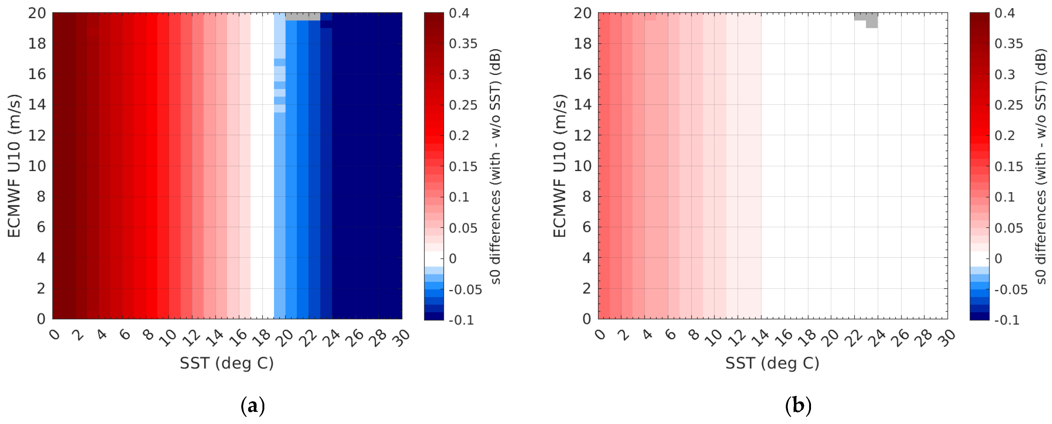
3. Correction for SST-Effect on s0 Based on a Sea Water Dielectric Constant Model

Vandemark et al. [15] proposed a first-order geophysical correction to mitigate this SST effect on s0. The main aspects are briefly summarized in the following section before applying it to estimate SST-related errors in U10. It is based on the reasonable assumption that nadir altimeter s0 behavior follows a quasi-optical backscattering model [58] since the specular reflection mechanism dominates. s0 can be expressed as: s0 |R²|/msseff. Here, note that s0 is in natural units (not in decibels (dB)). R is the Fresnel reflection coefficient of air to the sea surface for normal incidence. It is computed as: R = ( 1 ε ) /( 1 + ε ), where ɛ is the dielectric constant of sea water. The latter is related to the salinity, SSS, and temperature, SST, of the sea water and radar frequency by a model function, ε (SST, SSS). In the following, the semi-empirical ε model from Meissner and Wentz [59] at microwave frequencies is used. It is valid for an SSS ranging between 0 and 40 psu and an SST between −2° and 32 °C. msseff is the effective mean square slope of ocean surface roughness. It is an effective value and not a total one, because only waves several times longer than the radar wavelength are seen by the sensors [58]. This value is constant for a fixed sea surface roughness state. It is obvious here that the altimeter s0 is directly related to SST.
In the following, a point-to-point s0 correction is applied using coincident SST estimates. Each Jason-2 or AltiKa measurement is adjusted for reflectivity variation with an adapted scaling factor as described by the following steps:
1.
Convert s0 from dB (as provided in GDR) to a linear unit value, denoted as s0_lin: s0_lin = 10^(s0/10).
2.
Adjust each s0_lin with the scaling factor β = ρ(SST_ref)/ρ(SST), where ρ = |R²|, to obtain the corrected value denoted as s0_lin_corr: s0_lin_corr = s0_lin × β. SST_ref is taken at 18 °C and corresponds to the median value of the SST distribution over the 2015 period from the altimeter global dataset.
3.
Convert the s0_lin_corr from linear units back to a dB value to obtain s0_corr: s0_corr = 10 × log10 (s0_lin_corr).
Because the SSS impact is ~10 times lower than the SST effect, we neglect here the SSS influence and investigate only the SST effects, assuming a fixed SSS (35 psu). As reported by Vandemark et al. [15], this approach suppresses the ~3% and ~14% variations in s0 in the Ku and Ka band, respectively, due to the SST-dependent reflectivity change over the full range of SST variation.
The s0 biases associated with this SST dependence are shown in Figure 2 as a function of both SST and ECMWF wind force. There is no bias change with respect to the wind speed conditions as expected in the s0 correction design. The effect on the Ku band s0 is quite small; the biases increase when the SST decreases from 14 °C to 0 °C. The change barely reaches +0.12 dB in polar regions. Note that altimeter data for SSTs lower than 0 °C were removed from the assessment because of the potential contamination of the measurement by sea ice. In warmer conditions, there is no change in s0 above 15 °C because of the flatness of ρ behavior in the Ku band (as seen in Figure 1 of Vandemark et al. [15] publication). For the Ka band, besides (by definition) the zero-dB bias at 18 °C, the biases increase as the SST decreases towards 0 °C. They can reach +0.43 dB (almost 4 times the Ku band changes) in the coldest seas, while the s0 biases become gradually more negative towards warmer areas (SST > 18 °C) and are down to −0.16 dB at 30 °C. There is a change in s0 of almost 0.6 dB for the same wind conditions between polar regions and equatorial areas.

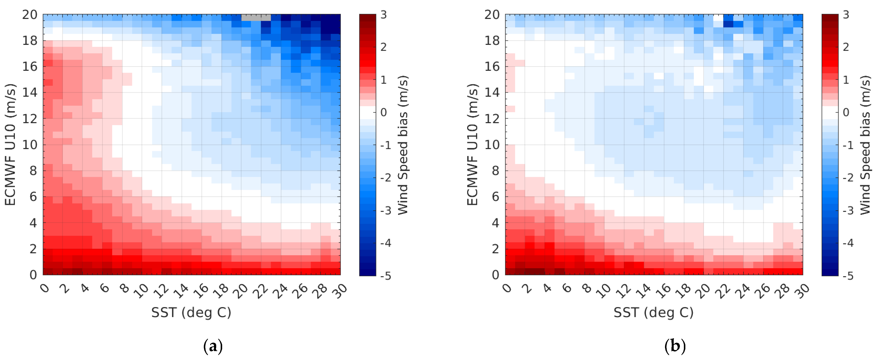
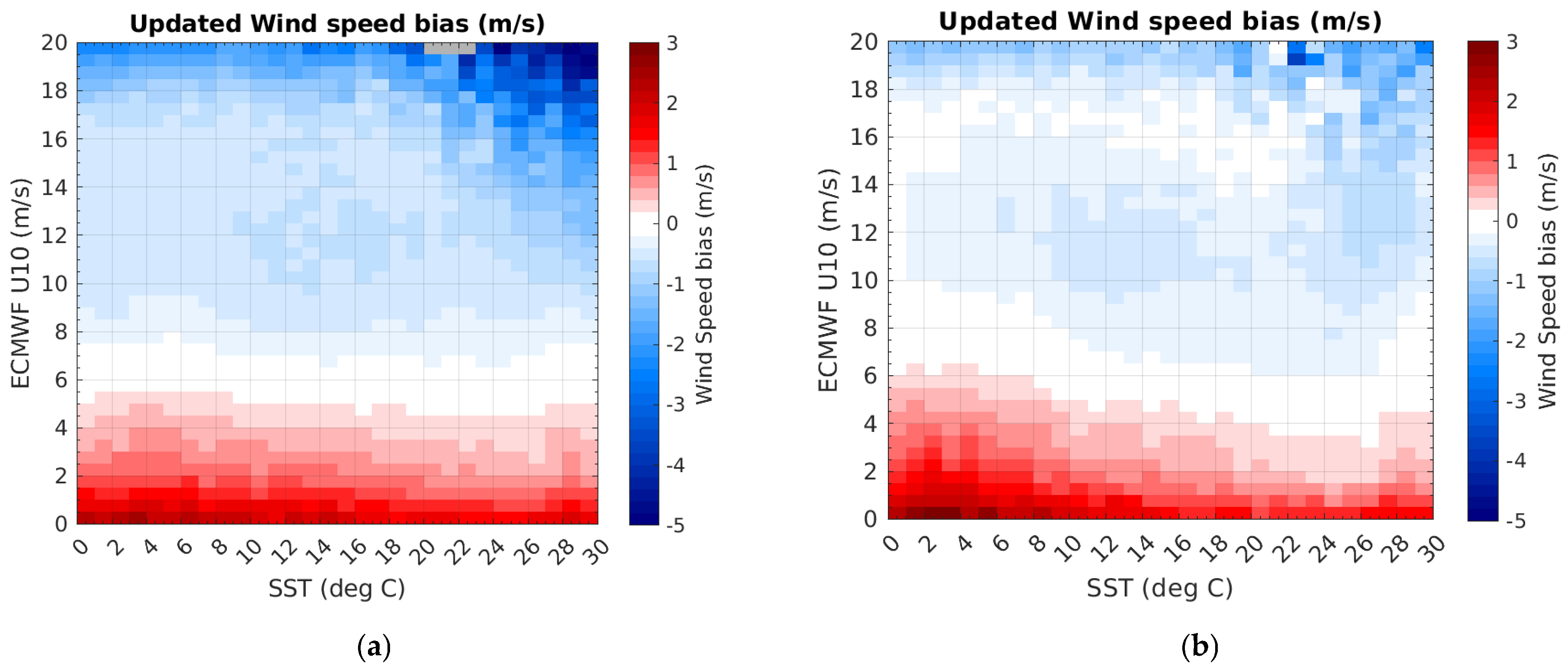
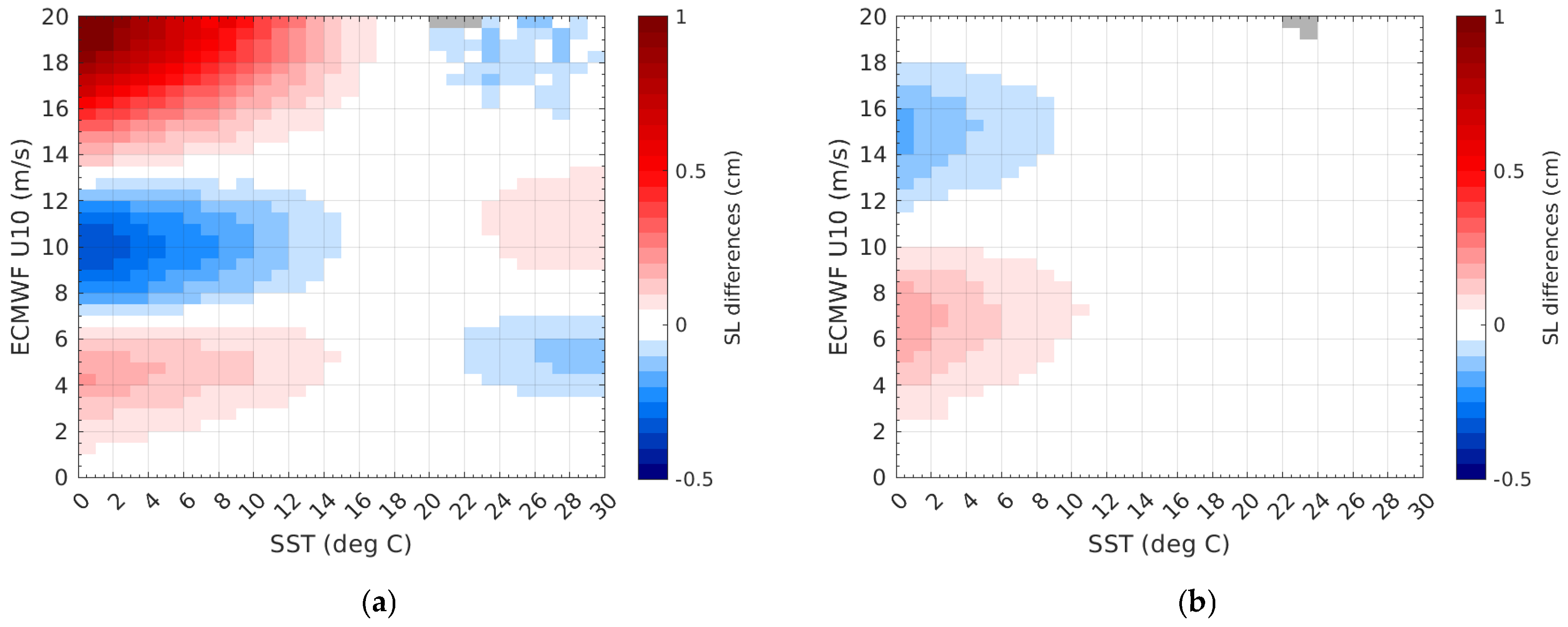
4. SST-Dependent Errors in Altimeter Wind and Sea Level

The SST-corrected s0 data were then used to retrieve wind speed by applying the operational models to produce new Jason-2 and AltiKa wind estimations. Their comparisons with the nominal values are shown in Figure 3. In the Ku band, the s0 differences in panel (b) translate to small differences in U10. They range between −0.6 and +0.05 m/s when going from the coldest seas to the warmest SST areas. These new Jason-2 data show a closer agreement with the ECMWF U10 data when one compares with Figure 1 results. Most of the SST-dependent errors seen in the nominal U10 values are well reduced by the ad hoc correction applied on the nominal s0 to adjust them. The new altimeter U10 biases are solely a function of the ECMWF U10 level under most conditions.
The improvement is more obvious and significant in the Ka band, as seen in panel (a) of Figure 3. The U10 biases related to the SST correction vary between −1.5 and +0.5 m/s when moving from the coldest SST to the opposite warmest conditions, especially for winds above 10 m/s. If most of the SST dependence in Figure 1 is removed, some residual features remain. In the Ka band, these concern situations where the SST is larger than 18 °C and winds are lying above 14 m/s, while for the Ku band, the differences with ECMWF data show a small residual SST dependence for SSTs colder than 10 °C and winds below 5 m/s.
These residual signatures might have originated from various sources: (1) errors related to the altimeter U10 model calibration or ECMWF model estimations that are larger for low- and high-wind conditions; (2) SST-dependent parameters that we did not consider here: surface tension and water kinematic viscosity, for example, which potentially may have influenced the observed s0 from the ocean; (3) errors in the dielectric constant errors; or perhaps (4) errors coming from the atmospheric attenuation correction applied on the altimeter s0 data under rainy and windy conditions and mostly affecting the Ka band s0 data in the equatorial band [60]. There are certainly also other errors that we omitted in this list here.
Indeed, besides the SST dependence in the dielectric constant of seawater that we accounted for, the SST physically also affect two other parameters which, potentially, may have influenced the observed s0 from the ocean: surface tension and water kinematic viscosity. They were both not considered here because they are more difficult to handle. Surface tension is relevant for roughness generation at low winds and has a linear dependency on the SST. As the SST decreases, surface tension increases, and less roughness will be generated for a given wind level. For higher winds, wave breaking will start to occur, and dynamic viscosity that decreases with the SST will come to play a role in dissipating the roughness generated by the breaking events. In Figure 1 and Figure 3, the observed biases also include such smaller effects and errors.
Finally, the impacts on the altimeter SL estimates were examined after the application of the operational 2D SSB model on each updated U10 values for the Jason-2 and AltiKa datasets, respectively. The results are provided in Figure 4. Correlated with the observed U10 biases in Figure 1, the largest SSB changes occur in the coldest seas (typically found above latitudes of 50°S or 65°N). For the Ku band data, the SST correction impact on the SSB estimations is small, within [−2, 2] mm, and this level of bias is typically considered negligible. Note, however, the bimodal change in the cold water SL estimate in the Ku band, where a positive bias is seen at moderate wind speeds, while a negative bias is observed at higher winds. This is due to nonlinear behaviors integrated in the SSB models and describe with SWH and U10 parameters.
Concerning the Ka band results shown in Figure 4, the impacts are greater, as expected, since the Ka band SSB behavior is more sensitive to changes in wind speed, and also because the U10 change with SST is larger. As for the Ku band, the effective SST correction impacts on SL also depends on wind speed, but in a different manner and mostly for the coldest and the warmest waters. The most significant changes (>5 mm) occur in polar regions, when the SST < 4 °C and the wind conditions are above 14 m/s. It can even reach 1 cm for stronger winds above 18 m/s.
The patterns in Figure 3 and Figure 4 are very different from each other because the main driving parameter for each algorithm is not the same, although they both rely directly or indirectly on s0 and SWH. In contrast to the wind speed modelling, where s0 is the main driver in the retrieval, for SSB correction, the primary driver is SWH, while U10 acts as a secondary factor. Moreover, as the SST and SWH data show anticorrelated variations and since the SSB behavior is also highly nonlinear, all add up to blur the SST signature in the SL records.
Figure 5 displays a geographical map of AltiKa SSB differences that translate directly as SL differences. The application of the SST correction on s0 removes large-scale biases of a few mm with respect to latitude. Negative bias values (−0.06 cm) are observed around the equator in the subtropical belts where the warmest waters (>26 °C) are located and trade winds flow with average speeds of ~5–6 m/s. The other negative bias region in blue is located between −40°S and −70°S, where SSTs are below 15 °C and westerly winds flow. In contrast, large positive biases occur over regions where cold SSTs and high winds are both present. This occurs mostly during austral winter when SSTs are the coldest (around 0 °C) and the pressure is low over the south pole, generating westerly winds above 15 m/s. Bias patterns are less defined in the Northern Hemisphere above 50°N because of the more changing wind flows. The patterns in the tropical belt are rather steady due to more stable SST and U10 conditions, while at latitudes closer to the poles, the air/sea conditions are more variable year-round. Overall, the SST-dependent errors on SL estimations are clear although weak at the mm level, on average, and display a large-scale trend between equatorial area and polar regions.
Even if global and regional MSL trends should not be affected by such an SST impact on s0 related to variations in the seawater dielectric constant, and this in the Ku and Ka bands, it may come into play when assessing uncertainties in computed regional trends (for example in polar regions) where estimate uncertainty must confront high frequency variability. At least in the Ka band and for SSTs below about 8 °C, the results also suggest that implicit coupling that occurs between the empirical altimeter wind speed and SSB models might be revisited to account for the SST impact on the backscatter. As climate change is amplified at the poles, this SST effect on altimeter s0 and its net impact on the SSB range correction and SL may slowly change in a mean sense alongside any polar region temperature trends.

5. Conclusions

The results reported by Vandemark et al. [15] clearly indicated that the retrieved Ka band wind speed estimation (from older GDR-T products) carries an SST-dependent error that can reach 1 m/s in polar regions when AltiKa and ECMWF U10 estimations are compared. They observed altimeter overestimation in cold water and underestimation for very warm SST and U10 larger than 5 m/s. They linked this error to SST through the Fresnel reflection coefficient dependency that is currently neglected in s0 data. This feature does more largely impact the Ka band s0 than that for the Ku band for altimetry applications. The application of their point-to-point ad hoc correction using collocated SST estimations leads to an obvious reduction in the wind speed bias that is especially evident in colder water.
In this paper, we confirmed their past results and went one step farther by evaluating the impact on SL records based on the most up-to-date algorithms and data (i.e., the latest GDR-F version for AltiKa) available at this time. The present analysis indicates that this SST effect translates to a wind speed estimation error of as much as 1.5 m/s and an error up to 1.0 cm in sea level records through SSB correction in the worst SST and U10 conditions. For comparison, in the Ku band, the errors in U10 and SL reach 0.6 m/s and 0.2 cm, respectively, when they are evaluated from Jason-2 data over the same period. However, the worst cases correspond to a relatively small fraction of the data population and should, therefore, lead to a negligible impact on global and regional MSL trend estimation. The application of this SST correction on s0 in this framework of repeated water level observations still looks interesting since it removes large-scale biases of a few mms. The recommendation is made to the space agencies in charge of altimetry product generation to consider this corrective step in their processing chain. In addition, SST represents an additional source of uncertainty that needs to be considered in the SL uncertainty budget.
Despite this, it is advised to keep providing the s0 data as nominally measured by altimeters in official products (i.e., without SST correction) to allow each user of altimeter s0 to evaluate the SST impact on their own developed applications. In the case of altimeter wind retrieval, SST has a significant impact on the Ka band estimations over colder seas that is much larger than on the Ku band ones. Thus, intercalibration between U10 products obtained from measuring systems operating at different frequencies should be handled with care to generate multi-mission wind products [61].
Finally, the SST impact is expected to be similar on s0 measurements, wind speed, and SSB estimations between standard nadir-pointing radar (AltiKa) and the innovative SWOT radar interferometer because only of the frequency choice. This has nothing to do with differences in radar technique. Moreover, Figure 6 provides an overview of how this AltiKa SST-related SSH error fits into SWOT’s total error budget described in Esteban-Fernandez’s document [62]. As seen, the oceanographic measurement requirement for SWOT science baseline is specified as a 1D (along-track) power spectral density for wavelengths below 1000 km and sets to be one order of magnitude below the ocean signal. The AltiKa SST-related error spectrum is largely below the SWOT baseline and represents only ~1% of the SWOT SSH error budget for all the wavelengths considered. This SST-dependent error can, thus, still be neglected for SWOT when considering its core objective, which is to characterize the ocean mesoscale and sub-mesoscale circulation at spatial resolutions of 15 km and larger. However, this may require consideration when comparing/combining the Ka-band Radar Interferometer (KaRIn) data (i.e., the scientific heart of the SWOT satellite) with the conventional Ku band nadir altimeter data, both operating on SWOT, on the topic of wind retrieval.

Author Contributions

Conceptualization, N.T., D.V., G.D. and F.B.-C.; methodology, N.T., D.V., G.D. and F.B.-C.; software, N.T. and D.V.; validation, N.T., D.V., F.B.-C. and G.D.; formal analysis, N.T., D.V., F.B.-C. and G.D.; investigation, N.T.; resources, N.T.; data curation, N.T.; writing—original draft preparation, N.T.; writing—review and editing, N.T., D.V., F.B.-C. and G.D.; visualization, N.T.; supervision, F.B.-C. and G.D.; project administration, F.B.-C., G.D. and D.V.; funding acquisition, F.B.-C. and D.V. All authors have read and agreed to the published version of the manuscript.

Funding

The French participation was funded by the Centre National d’Etudes Spatiales as part of the SALP project (200443). D.V.’s contribution was performed and funded under ST13301CQ0050/1332KP22FNEED0042 via NOAA-NESDIS Ocean Surface Topography Science team support.

Data Availability Statement

The altimetry data were downloaded from AVISO, available online: http://www.aviso.altimetry.fr, accessed on 1 January 2022. The NOAA OI SST V2 High Resolution Dataset data were provided by the NOAA PSL, Boulder, Colorado, USA, available online: https://psl.noaa.gov/data/gridded/data.noaa.oisst.v2.highres.html, accessed on 1 January 2022.

Acknowledgments

The authors would like to thank T. Meissner for providing the programs needed to implement the seawater permittivity model. We are also grateful to the anonymous reviewers for their thorough comments that helped to improve the paper.

Conflicts of Interest

The authors declare no conflict of interest.

References

  1. Bojinski, S.; Verstraete, M.; Peterson, T.C.; Richter, C.; Simmons, A.; Zemp, M. The Concept of Essential Climate Variables in Support of Climate Research, Applications, and Policy. Bull. Am. Meteorol. Soc. 2014, 95, 1431–1443. [Google Scholar] [CrossRef] [Green Version]
  2. Garcia-Soto, C.; Cheng, L.; Caesar, L.; Schmidtko, S.; Jewett, E.B.; Cheripka, A.; Rigor, I.; Caballero, A.; Chiba, S.; Báez, J.C.; et al. An Overview of Ocean Climate Change Indicators: Sea Surface Temperature, Ocean Heat Content, Ocean pH, Dissolved Oxygen Concentration, Arctic Sea Ice Extent, Thickness and Volume, Sea Level and Strength of the AMOC (Atlantic Meridional Overturning Circulation). Front. Mar. Sci. 2021, 8, 642372. [Google Scholar] [CrossRef]
  3. Domingues, C.M.; Church, J.A.; White, N.J.; Gleckler, P.J.; Wijffels, S.E.; Barker, P.M.; Dunn, J.R. Improved estimates of upper-ocean warming and multi-decadal sea-level rise. Nature 2008, 453, 1090–1093. [Google Scholar] [CrossRef] [PubMed]
  4. Mimura, N. Sea-level rise caused by climate change and its implications for society. Proc. Jpn. Acad. Ser. B 2013, 89, 281–301. [Google Scholar] [CrossRef] [Green Version]
  5. IPCC. IPCC Special Report on the Ocean and Cryosphere in a Changing Climate; Pörtner, D.H.O., Roberts, D.C., Masson-Delmotte, V., Zhai, P., Tignor, M., Poloczanska, E., Weyer, N.M., Eds.; IPCC: Geneva, Switzerland, 2019. [Google Scholar]
  6. Oppenheimer, M.; Glavovic, B.; Hinkel, J.; van de Wal, R.; Magnan, A.K.; Abd-Elgawad, A.; Cai, R.; Cifuentes-Jara, M.; Deconto, R.M.; Ghosh, T.; et al. Sea level rise and implications for low lying islands, coasts and communities. In IPCC Special Report on the Ocean and Cryosphere in a Changing Climate; Pörtner, D.H.O., Roberts, D.C., Masson-Delmotte, V., Zhai, P., Tignor, M., Poloczanska, E., Weyer, N.M., Eds.; IPCC: Geneva, Switzerland, 2019; pp. 321–446. [Google Scholar]
  7. WCRP Global Sea Level Budget Group. Global sea-level budget 1993–present. Earth Syst. Sci. Data 2018, 10, 1551–1590. [Google Scholar] [CrossRef] [Green Version]
  8. Cazenave, A.; Hamlington, B.; Horwath, M.; Barletta, V.R.; Benveniste, J.; Chambers, D.; Döll, P.; Hogg, A.E.; Legeais, J.F.; Merrifield, M.; et al. Observational Requirements for Long-Term Monitoring of the Global Mean Sea Level and Its Components Over the Altimetry Era. Front. Mar. Sci. 2019, 6, 582. [Google Scholar] [CrossRef]
  9. Widlansky, M.J.; Long, X.; Schloesser, F. Increase in sea level variability with ocean warming associated with the nonlinear thermal expansion of seawater. Commun. Earth Environ. 2020, 1, 9. [Google Scholar] [CrossRef]
  10. Guérou, A.; Meyssignac, B.; Prandi, P.; Ablain, M.; Ribes, A.; Bignalet-Cazalet, F. Current observed global mean sea level rise and acceleration estimated from satellite altimetry and the associated uncertainty. EGUsphere, 2022; preprint. [Google Scholar] [CrossRef]
  11. GCOS. Systematic Observation Requirements for Satellite-Based Data Products for Climate (2011 Update)—Supplemental Details to the Satellite-Based Component of the “Implementation Plan for the Global Observing System for Climate in Support of the UNFCCC (2010 Update)”; GCOS-154; WMO: Geneva, Switzerland, 2011. [Google Scholar]
  12. Ablain, M.; Philipps, S.; Urvoy, M.; Tran, N.; Picot, N. Detection of Long-Term Instabilities on Altimeter Backscatter Coefficient Thanks to Wind Speed Data Comparisons from Altimeters and Models. Mar. Geodesy 2012, 35, 258–275. [Google Scholar] [CrossRef]
  13. Donlon, C.J.; Cullen, R.; Giulicchi, L.; Vuilleumier, P.; Francis, C.R.; Kuschnerus, M.; Simpson, W.; Bouridah, A.; Caleno, M.; Bertoni, R.; et al. The Copernicus Sentinel-6 mission: Enhanced continuity of satellite sea level measurements from space. Remote Sens. Environ. 2021, 258, 112395. [Google Scholar] [CrossRef]
  14. Figerou, S.; Tran, N.; Bignalet-Cazalet, F.; Dibarboure, G.; Donlon, C. Uncertainties in SSB Modeling and Impact on MSL. In Proceedings of the 2022 Ocean Surface Topography Science Team Meeting, Venice, Italy, 31 October–4 November 2022. [Google Scholar]
  15. Vandemark, D.; Chapron, B.; Feng, H.; Mouche, A. Sea Surface Reflectivity Variation with Ocean Temperature at Ka-Band Observed Using Near-Nadir Satellite Radar Data. IEEE Geosci. Remote Sens. Lett. 2016, 13, 510–514. [Google Scholar] [CrossRef]
  16. Verron, J.; Sengenes, P.; Lambin, J.; Noubel, J.; Steunou, N.; Guillot, A.; Picot, N.; Coutin-Faye, S.; Sharma, R.; Gairola, R.M.; et al. The SARAL/AltiKa Altimetry Satellite Mission. Mar. Geodesy 2015, 38, 2–21. [Google Scholar] [CrossRef]
  17. Verron, J.; Bonnefond, P.; Andersen, O.; Ardhuin, F.; Bergé-Nguyen, M.; Bhowmick, S.; Blumstein, D.; Boy, F.; Brodeau, L.; Crétaux, J.F.; et al. The SAR-AL/AltiKa mission: A step forward to the future of altimetry. Adv. Space Res. 2021, 68, 808–828. [Google Scholar] [CrossRef]
  18. Bentamy, A.; Grodsky, S.A.; Elyouncha, A.; Chapron, B.; Desbiolles, F. Homogenization of scatterometer wind retrievals. Int. J. Clim. 2016, 37, 870–889. [Google Scholar] [CrossRef] [Green Version]
  19. Wang, Z.; Stoffelen, A.; Fois, F.; Verhoef, A.; Zhao, C.; Lin, M.; Chen, G. SST Dependence of Ku- and C-Band Backscatter Measurements. IEEE J. Sel. Top. Appl. Earth Obs. Remote Sens. 2017, 10, 2135–2146. [Google Scholar] [CrossRef]
  20. Jiang, H.; Zheng, H.; Mu, L. Improving Altimeter Wind Speed Retrievals Using Ocean Wave Parameters. IEEE J. Sel. Top. Appl. Earth Obs. Remote Sens. 2020, 13, 1917–1924. [Google Scholar] [CrossRef]
  21. Abdalla, S. Ku-Band Radar Altimeter Surface Wind Speed Algorithm. In Paper Presented at Envisat Symposium; European Space Agency: Montreux, Switzerland, 2007. [Google Scholar]
  22. Benassai, G.; Migliaccio, M.; Montuori, A.; Ricchi, A. Wave simulations through SAR COSMO-SkyMed wind retrieval and verification with buoy data. In Proceedings of the International Offshore and Polar Engineering Conference, Rhodes, Greece, 17–23 June 2012; pp. 1171–1178. [Google Scholar]
  23. Young, I.R. Seasonal variability of the global ocean wind and wave climate. Int. J. Climatol. 1999, 19, 931–950. [Google Scholar] [CrossRef]
  24. Liu, Q.; Babanin, A.; Zieger, S.; Young, I.; Guan, C. Wind and Wave Climate in the Arctic Ocean as Observed by Altimeters. J. Clim. 2016, 29, 7957–7975. [Google Scholar] [CrossRef]
  25. Ribal, A.; Young, I.R. 33 years of globally calibrated wave height and wind speed data based on altimeter observations. Sci. Data 2019, 6, 77. [Google Scholar] [CrossRef] [Green Version]
  26. Tournadre, J. Validation of Jason and Envisat Altimeter Dual Frequency Rain Flags. Mar. Geodesy 2004, 27, 153–169. [Google Scholar] [CrossRef]
  27. Quartly, G.D. Sea State and Rain: A Second Take on Dual-Frequency Altimetry. Mar. Geodesy 2004, 27, 133–152. [Google Scholar] [CrossRef] [Green Version]
  28. Tran, N.; Tournadre, J.; Femenias, P. Validation of Envisat Rain Detection and Rain Rate Estimates by Comparing with TRMM Data. IEEE Geosci. Remote Sens. Lett. 2008, 5, 658–662. [Google Scholar] [CrossRef]
  29. Gommenginger, C.P.; Srokosz, M.A.; Challenor, P.G.; Cotton, P.D. Measuring ocean wave period with satellite altimeters: A simple empirical model. Geophys. Res. Lett. 2003, 30, 2150. [Google Scholar] [CrossRef]
  30. Quilfen, Y.; Chapron, B.; Collard, F.; Serre, M. Calibration/validation of an altimeter wave period model and application to TOPEX/Poseidon and Jason-1 altimeters. Mar. Geod. 2004, 27, 535–549. [Google Scholar] [CrossRef]
  31. Kshatriya, J.; Sarkar, A.; Kumar, R. Determination of Ocean Wave Period from Altimeter Data Using Wave—Age Concept. Mar. Geod. 2005, 28, 71–79. [Google Scholar] [CrossRef]
  32. Vandemark, D.; Chapron, B.; Sun, J.; Crescenti, G.H.; Graber, H.C. Ocean wave slope observations using radar backscatter and laser altimeters. J. Phys. Oceanogr. 2004, 34, 2825–2842. [Google Scholar] [CrossRef]
  33. Frew, N.M.; Glover, D.M.; Bock, E.J.; McCue, S.J. A new approach to global airsea gas transfer velocity fields using dual-frequency altimeter backscatter. J. Geophys. Res. 2007, 112, C11003. [Google Scholar] [CrossRef] [Green Version]
  34. Glover, D.M.; Frew, M.N.; McCue, S.J. Air-sea gas transfer velocity estimates from the Jason-1 and TOPEX altimeters: Prospects for a long-term global time series. J. Mar. Syst. 2007, 66, 173–181. [Google Scholar] [CrossRef] [Green Version]
  35. Cheng, Y.; Tournadre, J.; Li, X.; Xu, Q.; Chapron, B. Impacts of oil spills on altimeter waveforms and radar backscatter cross section. J. Geophys. Res. Oceans 2017, 122, 3621–3637. [Google Scholar] [CrossRef] [Green Version]
  36. Abdalla, S. Ku-Band Radar Altimeter Surface Wind Speed Algorithm. Mar. Geod. 2012, 35, 276–298. [Google Scholar] [CrossRef] [Green Version]
  37. Abdalla, S. Calibration of SARAL/AltiKa Wind Speed. IEEE Geosci. Remote Sens. Lett. 2013, 11, 1121–1123. [Google Scholar] [CrossRef]
  38. Lillibridge, J.; Scharroo, R.; Abdalla, S.; Vandemark, D. One and two parameter wind speed models for Ka-band altimetry. J. Atmos. Ocean. Technol. 2014, 31, 630–638. [Google Scholar] [CrossRef]
  39. Gourrion, J.; VanDeMark, D.; Bailey, S.; Chapron, B.; Gommenginger, G.P.; Challenor, P.; Srokosz, M.A. A Two-Parameter Wind Speed Algorithm for Ku-Band Altimeters. J. Atmospheric Ocean. Technol. 2002, 19, 2030–2048. [Google Scholar] [CrossRef]
  40. Collard, F. Algorithmes de vent et période moyenne des vagues Jason-1 à base de réseaux de neurones, BO-021-CLS-0407-RF. Boost. Technol. 2005. [Google Scholar]
  41. Tran, N.; Vandemark, D.; Feng, H.; Guillot, A.; Picot, N. Updated Wind Speed and Sea State Bias Models for Ka-Band Altimetry, 2014 SARAL/AltiKa Workshop, Lake Constance, Germany. 2014. Available online: https://ostst.aviso.altimetry.fr/fileadmin/user_upload/tx_ausyclsseminar/files/Poster_PEACHI_ssb_tran2014.pdf (accessed on 1 January 2023).
  42. Gaspar, P.; Florens, J.-P. Estimation of the sea state bias in radar altimeter measurements of sea level: Results from a new nonparametric method. J. Geophys. Res. Oceans 1998, 103, 15803–15814. [Google Scholar] [CrossRef]
  43. Gaspar, P.; Labroue, S.; Ogor, F.; Lafitte, G.; Marchal, L.; Rafanel, M. Improving Nonparametric Estimates of the Sea State Bias in Radar Altimeter Measurements of Sea Level. J. Atmospheric Ocean. Technol. 2002, 19, 1690–1707. [Google Scholar] [CrossRef]
  44. Vandemark, D.; Tran, N.; Beckley, B.D.; Chapron, B.; Gaspar, P. Direct estimation of sea state impacts on radar altimeter sea level measurements. Geophys. Res. Lett. 2002, 29, 1. [Google Scholar] [CrossRef] [Green Version]
  45. Labroue, S.; Gaspar, P.; Dorandeu, J.; Zanifé, O.; Mertz, F.; Vincent, P.; Choquet, D. Nonparametric Estimates of the Sea State Bias for the Jason-1 Radar Altimeter. Mar. Geodesy 2004, 27, 453–481. [Google Scholar] [CrossRef]
  46. Feng, H.; Yao, S.; Li, L.; Tran, N.; Vandemark, D.; Labroue, S. Spline-Based Nonparametric Estimation of the Altimeter Sea-State Bias Correction. IEEE Geosci. Remote Sens. Lett. 2010, 7, 577–581. [Google Scholar] [CrossRef]
  47. Bignalet-Cazalet, F.; Couhert, A.; Queruel, N.; Urien, S.; Carrere, L.; Tran, N.; Jettou, G. SARAL/AltiKa Products Handbook. 2021. Available online: https://www.aviso.altimetry.fr/fileadmin/documents/data/tools/SARAL_Altika_products_handbook.pdf (accessed on 1 January 2023).
  48. Dumont, J.P.; Rosmorduc, V.; Picot, N.; Bronner, E.; Desai, S.; Bonekamp, H.; Figa, J.; Lillibridge, J.; Scharroo, R. OSTM/Jason-2 Products Hand-Book. 2017. Available online: http://www.aviso.altimetry.fr/fileadmin/documents/data/tools/hdbk_j2.pdf (accessed on 1 January 2023).
  49. Reynolds, R.W.; Smith, T.M.; Liu, C.; Chelton, D.B.; Casey, K.S.; Schlax, M.G. Daily high-resolution-blended analyses for sea surface temperature. J. Clim. 2007, 20, 5473–5496. [Google Scholar] [CrossRef]
  50. Donlon, C.J.; Martin, M.; Stark, J.; Roberts-Jones, J.; Fiedler, E.; Wimmer, W. The Operational Sea Surface Temperature and Sea Ice Analysis (OSTIA) system. Remote Sens. Environ. 2012, 116, 140–158. [Google Scholar] [CrossRef]
  51. Chelton, D.B. The Impact of SST Specification on ECMWF Surface Wind Stress Fields in the Eastern Tropical Pacific. J. Clim. 2005, 18, 530–550. [Google Scholar] [CrossRef] [Green Version]
  52. Ricchi, A.; Bonaldo, D.; Cioni, G.; Carniel, S.; Miglietta, M.M. Simulation of a flash-flood event over the Adriatic Sea with a high-resolution atmosphere–ocean–wave coupled system. Sci. Rep. 2021, 11, 1–11. [Google Scholar] [CrossRef] [PubMed]
  53. Meroni, A.N.; Parodi, A.; Pasquero, C. Role of SST Patterns on Surface Wind Modulation of a Heavy Midlatitude Precipitation Event. J. Geophys. Res. Atmos. 2018, 123, 9081–9096. [Google Scholar] [CrossRef]
  54. O’Neill, L.W.; Chelton, D.B.; Esbensen, S.K. Observations of SST-Induced Perturbations of the Wind Stress Field over the Southern Ocean on Seasonal Timescales. J. Clim. 2003, 16, 2340–2354. [Google Scholar] [CrossRef] [Green Version]
  55. O’neill, L.W.; Chelton, D.B.; Esbensen, S.K.; Wentz, F.J. High-Resolution Satellite Measurements of the Atmospheric Boundary Layer Response to SST Variations along the Agulhas Return Current. J. Clim. 2005, 18, 2706–2723. [Google Scholar] [CrossRef]
  56. O’neill, L.W.; Chelton, D.B.; Esbensen, S.K. The Effects of SST-Induced Surface Wind Speed and Direction Gradients on Midlatitude Surface Vorticity and Divergence. J. Clim. 2010, 23, 255–281. [Google Scholar] [CrossRef]
  57. Miglietta, M.M.; Mazon, J.; Motola, V.; Pasini, A. Effect of a positive Sea Surface Temperature anomaly on a Mediterranean tornadic supercell. Sci. Rep. 2017, 7, 12828. [Google Scholar] [CrossRef] [Green Version]
  58. Jackson, F.C.; Walton, W.T.; Hines, D.E.; Walter, B.A.; Peng, C.Y. Sea surface mean square slope from Ku-band backscatter data. J. Geophys. Res. 1992, 97, 11411–11427. [Google Scholar] [CrossRef]
  59. Meissner, T.; Wentz, F. The complex dielectric constant of pure and sea water from microwave satellite observations. IEEE Trans. Geosci. Remote Sens. 2004, 42, 1836–1849. [Google Scholar] [CrossRef] [Green Version]
  60. Verron, J.; Bahurel, P.; Caubet, E.; Chapron, B.; Crétaux, J.F.; Eymard, L.; Leprovost, C.; Le Traon, P.Y.; Phalippou, L.; Rémy, F.; et al. Altika—A micro-satellite Ka-band altimetry mission. In Proceedings of the 52th International As-tronautical Congress, Toulouse, France, 1–5 October 2001. [Google Scholar]
  61. Grodsky, S.A.; Kudryavtsev, V.N.; Bentamy, A.; Carton, J.A.; Chapron, B. Does direct impact of SST on short wind waves matter for scatterometry? Geophys. Res. Lett. 2012, 39. [Google Scholar] [CrossRef] [Green Version]
  62. Esteban-Fernandez, D. SWOT Mission Performance and Error Budget, NASA/JPL Document (Reference: JPL D-79084); Jet Propulsion Laboratory: Pasadena, CA, USA, 2013. Available online: https://swot.jpl.nasa.gov/system/documents/files/2178_2178_SWOT_D-79084_v10Y_FINAL_REVA__06082017.pdf (accessed on 1 January 2023).
Figure 1. Wind speed biases between altimeter and ECMWF model estimations as a function of SST and ECMWF wind conditions, from collocations with AltiKa (a) and Jason-2 (b).
Remotesensing 15 03235 g001
Figure 2. s0 variations (in dB) related to the use of the SST ad hoc correction as a function of SST and ECMWF wind conditions, from AltiKa (a) and Jason-2 datasets (b). If the amount of data in a bin is less than 10, it is masked as grey.
Remotesensing 15 03235 g002
Figure 3. Same as Figure 1 but with the updated altimetric U10 that uses the SST correction on s0. (a) for AltiKa and (b) for Jason-2.
Remotesensing 15 03235 g003
Figure 4. Same as Figure 2 (a) for AltiKa and (b) for Jason-2, but now showing the SSB-controlled differences in altimeter sea level estimation change (in cm) due to SST correction of the altimeter backscatter and then wind speed.
Remotesensing 15 03235 g004
Figure 5. Map of the differences in Altika SL estimations (in cm) when considering or not the SST ad hoc correction in s0.
Remotesensing 15 03235 g005
Figure 6. SWOT SSH error spectrum requirement (red curve) for the science baseline as a function of wavenumber along with the SST-related errors in SSH spectrum (black curve) evaluated from AltiKa.
Remotesensing 15 03235 g006
Disclaimer/Publisher’s Note: The statements, opinions and data contained in all publications are solely those of the individual author(s) and contributor(s) and not of MDPI and/or the editor(s). MDPI and/or the editor(s) disclaim responsibility for any injury to people or property resulting from any ideas, methods, instructions or products referred to in the content.

