
ICESat-2 Bathymetric Signal Reconstruction Method Based on a Deep Learning Model with Active–Passive Data Fusion

1
College of Oceanography and Space Informatics, China University of Petroleum (East China), Qingdao 266580, China
2
First Institute of Oceanography, Ministry of Natural Resources, Qingdao 266061, China
3
Technology Innovation Center for Ocean Telemetry, Ministry of Natural Resources, Qingdao 266061, China
*
Author to whom correspondence should be addressed.
Remote Sens. 2023, 15(2), 460; https://doi.org/10.3390/rs15020460
Submission received: 21 November 2022
/
Revised: 29 December 2022
/
Accepted: 9 January 2023
/
Published: 12 January 2023
(This article belongs to the Special Issue Theory and Applications of Satellite Laser Altimetry in Oceanography and Limnology)
Abstract
:When carrying out SDB (satellite-derived bathymetry) in island area based on ICESat-2 (Ice, Cloud, and land Elevation Satellite 2) data, it is often found that the ICESat-2 bathymetric signals are partially missing due to the influence of thick aerosols such as clouds and fog. This not only hinders the accurate extraction of the along-track underwater topography, but also restricts the active–passive fusion bathymetry based on ICESat-2 data and multi/hyperspectral remote sensing images. In this paper, aiming at the partially missing ICESat-2 bathymetric signals, combined with passive optical remote sensing images, and based on an LSTM (long short-term memory) deep recurrent neural network model, an ICESat-2 bathymetric signal reconstruction method based on active–passive data fusion is proposed. It is found that this method can effectively reconstruct the local missing bathymetric signals. When the reconstructed ICESat-2 bathymetric data are applied to carry out active–passive fusion and bathymetric inversion, the accuracy indices are better than those of the inversion results of the data with partial missing signals, and the performance is comparable to that of the original data without missing data, which is of great value for the bathymetric application of ICESat-2 data in island and reef areas.
1. Introduction
Shallow-water bathymetry around islands and reefs is of great significance in coastal zone construction, navigation safety, and resource development [1], and how to obtain underwater topographic information in such areas with low cost, high accuracy, and high efficiency has always been a major concern for relevant researchers. Since the 1960s, with the continuous launch of multi/hyperspectral remote sensing satellites and the development of relevant bathymetric models, SDB (satellite-derived bathymetry) is becoming a cost-effective way to explore shallow underwater topography in island areas [2]. Semi-theoretical and semi-empirical models [3,4,5,6] and statistical models [7,8] are currently widely used in SDB works based on passive optical images, but they require high-precision measured depth data as their basis, which restricts the application of SDB in islands and reef areas that are not easily accessible to ships. Theoretical analytical models [9,10,11] generally do not rely on measured depth data, but the need to obtain the optical parameters of the water column during the construction of the model, along with the complexity of the calculations, limits the application of such models. ICESat-2 (Ice, Cloud, and land Elevation Satellite 2) [12,13] was launched in 2018, and its mounted spaceborne photon-counting LiDAR—i.e., ATLAS (Advanced Topographic Laser Altimeter System)—can actively detect shallow-water depth information. As a novel active in situ data source, it has been widely used in SDB works [14,15,16,17,18] in recent years. Some researchers further fuse ICESat-2 bathymetric data with multispectral remote sensing images to carry out bathymetric studies based on active–passive data fusion [8,19,20,21], which compensates for the shortcomings of ICESat-2 data that are only distributed along a straight track.
When using ICESat-2/ATLAS to carry out shallow-water bathymetry, the work is usually based on the ATL03 dataset [22] of the ICESat-2 mission. Most of the existing ICESat-2 SDB studies focus on how to accurately identify the signal clusters that can characterize the surface elevation and seafloor topography from the ATL03 point cloud data containing complex background noise. Then, through refraction correction [14] and tidal correction, accurate water depth control points in the study area can be obtained, but this process is highly susceptible to atmospheric conditions. The 532 nm pulsed laser emitted by ATLAS has a much lower penetration power for aerosols than its ability in water, which makes it difficult for the laser emitted by ATLAS to penetrate the aerosols and reach the sea surface in regions with high AOD (aerosol optical depth). In the ATL03 point cloud, this process is manifested as signal strips that fail to continuously present underwater topographic features due to local missing signals. For ICESat-2 SDB, this situation, as shown in Figure 1, poses two potential problems: firstly, parts of the sea areas are missing the adjacent along-track bathymetric control points, which will inevitably affect the water depth inversion accuracy of local sea areas; secondly, for the continuously rising/descending sea areas, the absence of underwater topography along the ICESat-2 track means that the control information of some water depth segments is missing, which restricts the bathymetric accuracy in corresponding sea areas.
Focusing on the problem of partially missing ICESat-2 bathymetric signals due to the influence of thick aerosols, this paper proposes an ICESat-2 bathymetric signal reconstruction method based on an LSTM (long short-term memory) deep learning model where active–passive data fusion is applied. Based on the multispectral passive optical remote sensing images of the sea areas with missing bathymetric signals and the adjacent ICESat-2 active bathymetric points, the LSTM deep learning model was applied to repair the missing bathymetric signal along the track with active–passive data fusion (active data provide water depth control points, while passive data provide spectral information). In addition, the log-ratio information of the three visible-light bands in the multispectral images were introduced as additional input features of the deep learning model to ensure the high-precision bathymetric inversion of sea areas where some water depth segment information was missing. In this paper, a total of three study areas around Dongdao Island and Shanhu Island in the Xisha Islands, China and Oahu Island in Hawaii were selected, and three sets of ICESat-2/ATL03 data were partially deleted manually to simulate the scenario of missing bathymetric data for validation experiments. The results showed that the proposed method can effectively reconstruct the local missing bathymetric signals, and the spatial distribution of the reconstructed signals was essentially consistent with the original data without data missing. Through the establishment of a four-band log-linear model, Stumpf log-ratio model, SVM (support-vector regression), model and DBN (deep belief network) model, the inversion accuracy before and after signal reconstruction was compared. It was found that the signals reconstructed by the proposed method effectively improved the accuracy of water depth inversion, achieving results close to the accuracy of inversion performed using the original data without data missing.
2. Data and Study Areas
2.1. Active/Passive Data
2.1.1. Active Data: ICESat-2 LiDAR Data
The ICESat-2 satellite was launched in September 2018, mounting the first spaceborne photon-counting LiDAR, known as ATLAS, which is a micro-pulse, high-frequency laser altimetry system. ICESat-2 has an orbit height of nearly 500 km, with an orbital inclination of 92° and a total of 1387 fixed RGTs (reference ground tracks) worldwide, and with a repeat cycle of 91 days. ATLAS is designed with six laser beams, which are arranged in three parallel groups along the track direction, each group containing a strong beam and a weak beam, with an energy ratio of 4:1. The system continuously emits 532 nm photon pulses at a frequency of 10 kHz and can acquire overlapping light spots with an along-track spacing of 0.7 m and a footprint of about 10 m [23]. The main information of ICESat-2/ATLAS is shown in Table 1.
Since the 532 nm laser has a strong penetration capability in nearshore water, it is suitable for shallow bathymetry using the ICESat-2/ATL03 dataset [22], which contains longitude, latitude, elevation, and other information for all of the photons. Figure 1 shows a group of real ICESat-2/ATL03 along-track point clouds, and it can be seen that the photons emitted by ATLAS gather into obvious strip-like photon clusters at the sea surface and the seafloor, respectively, providing a reliable active data source for shallow bathymetry. However, the 532 nm laser has poor ability to penetrate aerosols, and the Earth observation capability of ICESat-2 is greatly reduced when there are thick aerosols such as clouds and fogs. As shown in Figure 1, within the range of about 2500 m to 3000 m along the track, due to the influence of thick aerosols suspected to be clouds at high altitudes, almost all sea-surface and seabed signals in this range are missing, and it is difficult to extract the underwater terrain in this sea area. In this study, in order to verify the availability of the proposed reconstruction method, four ICESat-2/ATL03 point cloud data of the latest version (Version 5) are introduced, and their specific information is described in Section 2.2. In addition, since the strong beam has four times the energy of the weak beam in a given group, the point cloud data of the strong beams usually have higher signal-to-noise ratio and bathymetric capability, and this study was carried out based on the strong beams of the four data.
2.1.2. Passive Data: Multispectral Remote Sensing Imagery
Multispectral remote sensing is the most widely used passive optical remote sensing technology, with the advantages of wide coverage, low acquisition cost, rich data accumulation, and mature research of related models [1,2]. Multispectral remote sensing bathymetric inversion establishes the relationship between remote sensing image radiance values and water depth values by various means, such as theoretical analytical models, semi-theoretical and semi-empirical models [3,4,9], statistical models [7], etc., which can obtain large coverage of shallow seawater depth at low costs. After more than half a century of development, multispectral remote sensing bathymetry has become a mainstream shallow water depth detection method.
In this study, the spectral information provided by multispectral satellite remote sensing images is the main basis for the ICESat-2 bathymetric signal reconstruction. Based on the data accumulation and the experimental needs of each study area, four different sources of multispectral remote sensing images are used. They are derived from the WorldView-2 satellite of DigitalGlobe Corporation, the China-made GF-2 and GF-1 satellites, and the ESA’s Sentinel-2A satellite, respectively. Their spatial resolutions in the visible spectral band are 2 m, 3.2 m, 8 m, and 10 m, respectively, which can meet the needs of active–passive fusion with ICESat-2 data (the footprint diameter is about 10 m). The main information of these multispectral remote sensing data is shown in Table 2.
2.2. Study Areas
In order to fully verify and discuss the method in this paper, three study areas were selected for this study. Study area A is located near Dongdao Island of the Xisha Islands, China, which is rich in coral reef resources and has clear water suitable for shallow optical bathymetry. In this study area, WorldView-2, GF-2 PMS (panchromatic/multispectral sensor), and GF-1 PMS multispectral images were used as passive data, and the range is shown in Figure 2a. Meanwhile, ICESat-2 data (ATL03_20181116062310_07430101_005) from this area were used as the active data. Based on our previous study [16], the green and red points in Figure 2a are the bathymetric control points extracted based on these ICESat-2 data, where the red part is manually removed to simulate the scene of the missing ICESat-2 bathymetry signals. The yellow “+” in the figure represents the sampled validation data in this study area, i.e., the in situ bathymetric sample points obtained by shipborne sonar with the support of the National High-tech Research and Development Program of China. These bathymetric points can meet the accuracy requirements for TVU and THU in exclusive order according to the IHO (International Hydrographic Organization)’s S-44 standard [24], and their spatial resolution is better than that of ICESat-2, making them suitable for accuracy validation.
Study area B is located near Shanhu Island, Xisha Islands, China, and a GF-2 multispectral remote sensing image acquired in this sea area was used as the passive data, as shown in Figure 2b. Meanwhile, ICESat-2 data (ATL03_20190222135159_08570207_005) in this sea area were used as the active data; the corresponding ICESat-2 bathymetric control points and the parts to be removed are shown in the green and red points in Figure 2b, respectively. Due to the lack of sufficient in situ measured bathymetry data near Shanhu Island, another set of ICESat-2 data (ATL03_20191020141751_03620501_005) passing through this island was used to verify the inversion accuracy of this study area, as shown by the yellow “+” in Figure 2b.
Study area C is located near Oahu Island, Hawaii. In this study, Sentinel-2A multispectral remote sensing images acquired in this area were used as passive data, and the extent of the study area is shown in Figure 2c. Meanwhile, the ICESat-2 data (ATL03_20200106043104_01600601_005) were used as the active data, and the corresponding ICESat-2 bathymetric control points and the removed parts are shown in Figure 2c. The validation data marked by yellow “+” are ALB (airborne LiDAR bathymetry) data collected by the SHOALS (Scanning Hydrographic Operational Airborne Lidar Survey) system [25], which is sourced from the U.S. Naval Oceanographic Office, U.S. Geological Service, U.S. Army Corps of Engineers, and Honolulu District. The maximum depth can reach 40 m, the vertical error is less than 0.15 m, and the point spacing between the bathymetry data is 3–15 m. There are millions of ALB bathymetry points in this study area, and about 2000 of them were randomly sampled for accuracy validation. The detailed information of these three areas is shown in Table 3.
In addition, in order to eliminate the influence of tides on the bathymetric inversion, historical tide data from tidal stations closest to these three study areas were selected, and tidal corrections were made for the multispectral data, ICESat-2 data, and in situ data, respectively. For study areas A and B, historical tidal data from the tidal station located at Yongxing Island were used; for study area C, historical tidal data obtained in Waianae, Oahu Island were used.
3. Methods
3.1. ICESat-2 Bathymetric Signal Reconstruction Deep Learning Model
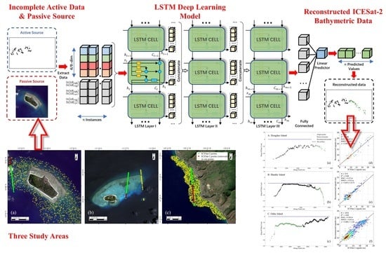
For the missing ICESat-2 bathymetric signals due to thick aerosol cover, the key to repairing them is to accurately mine the passive optical characteristics of the missing points to supervise the inversion of the water depth in these regions. To this end, we introduced multispectral passive optical remote sensing images and carried out water depth inversion with active–passive data fusion to establish the mapping relationship between water depth values and remote sensing spectral features along the ICESat-2 track. However, ICESat-2 bathymetric data usually have a large spatial coverage, and the optical properties of the water column and the types of bottom sediments vary significantly, making it difficult to construct an analytical or a semi-analytical model to calculate water depth values along the track. Therefore, based on the LSTM (long short-term memory) deep learning model [26], we established the along-track mapping relationship between passive remote sensing spectral characteristics and the active LiDAR bathymetric data, and then we carried out the active–passive fusion reconstruction of the ICESat-2 bathymetric signals.
The LSTM model has strong representation learning ability and model generalization, enabling it to effectively summarize complex features and conditions in practical problems, and it usually has sufficient model capacity to adequately fit the mapping relationships to be determined. Compared with the traditional neural networks that treat the information of each band in the spectral dimension as discrete individuals, the LSTM model can take into account the individual features of each band and the sequence features of the entire spectral dimension at the same time, due to its recurrent network structure. Unlike classical neural network models, LSTM adopts a special neural unit structure—the LSTM cell, which introduces a gate structure to preserve historical information and long-term state. The gate structure is implemented by a sigmoid function and a point multiplication operation to control the flow of information, and it does not provide additional information. There are three types of gates in an LSTM cell: the input gate, forget gate, and output gate. The input gate is used to update the cell state, the forget gate determines which information to discard or retain, and the output gate is used to determine the value of the next hidden state that contains information from previous inputs. These can be summarized in a general representation:
where —the sigmoid activation function used in classical neural networks—while and represent the weight matrix and bias vector of the network, respectively, which will gradually approach their optimal values during the training process of the model.
Figure 3 shows the internal structure of an LSTM cell. At moment , the input of the memory cell includes the hidden layer state variable of the previous moment, the memory cell state variable , and the input information at the current moment; then, the data pass through the forget gate , input gate , and output gate , and these three control mechanisms can determine the hidden layer state variable and memory cell state variable at time ; and are then transmitted to the next time for further calculation.
The model structure of this paper is shown in Figure 4, which contains three LSTM layers with a large number of LSTM units inside, a fully connected layer, and a linear layer for outputting predicted water depth values. Our model adopts a three-layer hidden layer structure of (200-200-200), the loss function is MAPE (mean absolute percentage error), the optimizer function uses Adam [27] (adaptive moment estimation), and the batch size is a fixed value of 64. In order to utilize the representation learning ability of deep learning, we put all available ICESat-2 bathymetry data into the model except for those that were manually removed. Meanwhile, in order to fully exploit the physical characteristics of multispectral optical remote sensing bathymetry inversion, the input of the model has the following three log-ratio features introduced based on related studies [4], in addition to the features of each spectral band in the passive remote sensing images:
where is the parameter to be fitted in the log-ratio model, and in this study is taken as a fixed value of 1000 [5,6]. is the reflectance of the visible bands , , and . As shown in Figure 4, these three log-ratio features, together with the band features of the passive optical image, constitute the input data for the model.
3.2. The Overall Framework of ICESat-2 Bathymetric Signal Reconstruction
The overall framework of the ICESat-2 bathymetric signal reconstruction based on active–passive data fusion in this paper is shown in Figure 5, consisting of three parts: The first part carries out data pre-processing. For the ICESat-2 ATL03 active data, it is necessary to extract bathymetric signals based on the ICESat-2 bathymetric signal extraction method. This process in this study is based on our previously proposed signal extraction algorithm [16], which can effectively separate bathymetric signals and noises from point clouds containing a large amount of noise. Since the geographical coordinates of the ATL03 data are calculated only under the condition of laser propagation in an air medium, to obtain accurate water depth information, refraction correction is required for the underwater part of the point cloud. This paper adopts a classical and effective refraction correction algorithm proposed by Parrish [14]. Based on the ground angle “ref_elev” of each photon given in the ATL03 data, the incident angle when the laser enters the water column is calculated. Then, according to Snell’s law, the elevation correction of each photon in the extracted results is performed to correct the refraction effort in the water column.
In addition, since the acquisition times of the active data and passive data are not the same, in order to eliminate the errors caused by tidal variations, it is also necessary to perform tidal correction on the ICESat-2 bathymetry values based on historical tidal data recorded at tidal stations near the study area. In order to verify the reconstruction effect of the bathymetric signals, we manually removed a section of the original complete ICESat-2 bathymetric data along the track for verification, and the remaining part was used to simulate the data with missing signals. For passive multispectral remote sensing data, radiometric calibration, atmospheric correction, and georeferencing were carried out in sequence, and we then fused them with the simulated active data with missing signals for the LSTM deep learning model’s training in the second part.
After the training of the signal reconstruction deep learning model, the model was applied to the along-track regions with missing data. In this paper, we applied the model directly to the extracted water depth sample points in the previous stage to generate the reconstructed bathymetric points at the same location as the manually removed points, which is convenient for comparison and analysis with the validation data. In the practical signal reconstruction work, the sample points were selected at intervals of 0.7 m along the track with reference to the sampling frequency of the ICESat-2 satellite. After that, the reconstructed data in the manually removed region were combined with the original ICESat-2 data to obtain the complete bathymetric data after reconstruction. The reconstructed data were used as control points for various water depth inversion models (such as log-linear, Stumpf, SVR, DBN, etc.), and the in situ data in the study area were used as checkpoints for validation. Finally, to evaluate the value of data reconstruction in water depth inversion, the inversion results were compared with the results obtained by applying the bathymetric data with manual removal and the original data without partially missing signals.
4. Experiments and Analysis
4.1. Experimental Settings
4.1.1. Inversion Models for Validation
In order to fully verify the effectiveness of the proposed ICESat-2 bathymetric signal reconstruction method in water depth inversion, four typical multispectral bathymetric inversion models were established: the log-linear model, Stumpf log-ratio model, SVR model, and DBN model. The first two are classical semi-theoretical and semi-analytical models, which have been widely used in the field of multispectral bathymetric inversion. The latter two are representative machine learning models that can also be effectively used for water depth inversion, while DBN is also a classical deep learning model.
- (1)
- Log-linear model
The log-linear model represents the radiance received by the optical remote sensor as the sum of the reflected radiance of the seafloor and the deep-water radiance, which is expressed as follows:
where are the parameters to be regressed, is the water depth value. , is the radiance value of band after atmospheric correction and solar flare correction, and is the radiance value of band in deep water.
- (2)
- Stumpf log-ratio model
In order to prevent the situation where the difference between the radiance received by the sensor and the radiance in deep water is negative in the log-linear model, Stumpf [4] proposed the following log-ratio model:
where , , and are the parameters to be regressed, while is the reflectance of the corresponding band. This model usually works better in sea areas where the radiance values are low.
- (3)
- SVR (support-vector regression) model
SVR is a variant of SVM (support-vector machine) used in regression analysis. Unlike SVM, which causes the majority of the sample points to lie on the outside of two decision boundaries by finding a suitable separating hyperplane, the SVR model expects most of the samples to lie inside the decision boundaries. In this paper, the SVR model uses the RBF (radial basis function) kernel, which makes it effective in handling the nonlinear multiple regression problem of water depth inversion.
- (4)
- DBN (deep belief network) model
DBN [28] is a classical deep learning model, whose basic unit is the RBM [29] (restricted Boltzmann machine). An RBM can be regarded as a Markov random field with an undirected graph structure, containing visible and hidden layers connected by weight matrices. A DBN solves the problem that traditional BP (backpropagation) models find it difficult to train deep neural networks, and it can adequately deal with regression problems such as water depth inversion.
4.1.2. Accuracy Indices
In this study, the RMSE (root-mean-square error), MAE (mean absolute error), and MRE (mean relative error) were used to evaluate the accuracy of the water depth inversion results, and the effects of water depth inversion before and after ICESat-2 data reconstruction were compared and analyzed. These three indices can show the error between the observed values and the predicted values—the smaller their values, the better the inversion.
where and are the predicted water depth value and the observed value of the th point, respectively, while is the total number of bathymetric points involved in the accuracy evaluation.
4.2. Experimental Results
After manually removing some data from the ICESat-2 bathymetric data described above, combined with multispectral passive optical remote sensing images, the bathymetric signal reconstruction experiments were carried out in the three study areas of Dongdao Island, Shanhu Island, and Oahu Island; the experimental results are shown in Figure 6. The black points in the figure are the bathymetric signals that were not deleted, which were used to simulate the ICESat-2 bathymetric signals with missing data and were also used as the training data for the reconstruction experiment. The gray points are the manually deleted ICESat-2 bathymetry signals in the original data, which were used to compare and verify the effects of signal reconstruction. The green points are the reconstructed signals obtained by the LSTM reconstruction model in this paper, and the ICESat-2 bathymetric data after reconstruction were obtained by merging the green point set with the black point set.
Figure 6a–c show the reconstruction results of study area A (Dongdao Island), study area B (Shanhu Island), and study area C (Oahu Island), respectively. Figure 6d–f show the scatterplots of the reconstructed signals versus the original ICESat-2 signals in these three study areas, respectively, and the relevant accuracy indices are also labeled in these plots. As can be seen in the figures, the reconstruction results of study areas B and C are very good, and the change trend of water depth is essentially consistent with the original ICESat-2 bathymetric data, while the signals are generally concentrated and smooth, allowing them to accurately portray the along-track topographic characteristics in this area. From the scatterplots, it can be seen that most of the signals in these two study areas are gathered near the fitting line, and a small amount of the signals are divergent. Their determination coefficients () are 0.88 and 0.89, respectively, and their RMSE is 0.52 m and 0.65 m, respectively. For study area A, there are a large range of coral reefs distributed, especially in the shallow part of the middle section, where the terrain changes drastically and the ICESat-2 data are relatively scattered, making it difficult to reconstruct the removed data in this shallow area. The reconstructed signals in this part are relatively divergent, with some outliers appearing, but the overall trend still conforms to the distribution of the real ICESat-2 data, which also have high reliability. The and RMSE of the reconstructed signals in study area A are 0.86 and 0.89 m, respectively.
After signal reconstruction, four multispectral water depth inversion models (log-linear, Stumpf log-ratio, SVR, and DBN models) were selected to carry out water depth inversion based on the ICESat-2 bathymetric data with partially missing signals (“removed” in Table 4), the original ICESat-2 bathymetric data before manual removal (“original” in Table 4), and the ICESat-2 bathymetric data after signal reconstruction (“reconstructed” in Table 4) by the proposed method. The accuracy of the water depth inversion is shown in Table 4.
As can be seen from Table 4, for all three study areas, the data with partially missing signals achieved relatively poor results in all sets of inversion experiments, and the RMSE, MAE, and MRE indices were generally inferior to the results of the other two comparison datasets. However, after the proposed method based on active–passive data fusion was used to reconstruct the bathymetric data, almost all indices were better than those of the data before reconstruction, and the accuracy was comparable with the inversion with the original data containing complete bathymetric information. Especially for the experiments using the DBN deep learning model, the inversion results of the reconstructed bathymetric data were even slightly better than those of the original bathymetric data. This is because the signal reconstruction with active–passive fusion is supervised by passive optical remote sensing images, whose information it contains. The reconstructed bathymetric data usually have more correlation with remote sensing images than the original ICESat-2 bathymetric data, reducing the small error caused by the spatial and temporal matching of active–passive data in the inversion stage.
Figure 7 shows the inversion results of applying the three groups of bathymetric data with the four models in the Dongdao Island study area. Among them, Figure 7a–d show the inversion results of data with partial manual deletion under the log-linear model, Stumpf model, SVR model, and DBN model, respectively. Figure 7e–h show the inversion results of the original data in the four models, respectively, while Figure 7i–l show the inversion results of the reconstructed data in the four models, respectively. It can be seen from the results that the inversion results of the three groups of data in each model were relatively close, and the reconstructed data maintained the reliability of the inversion effect. Figure 8 shows the inversion results in the Shanhu Island study area. In this group of experiments, the results of the reconstructed data were also close to the results of the original data without data missing, and slightly better than the results of the data with partial manual deletion. In contrast, the selection of the water depth inversion model had a greater impact on the inversion results, as discussed specifically in Section 5.3.
Figure 9 shows the water depth inversion results of the Oahu Island study area, and the impact of data reconstruction on the water depth inversion is more obvious due to the relatively large range of manually deleted data in this area (as shown in Figure 6c). In this group of experiments, the removed data not only affected the inversion effect of local areas, but also affected the overall inversion ability of the study area. The results with missing data were generally underpredicted in deep-water areas. For some models, the maximum bathymetric capability was also significantly affected. For example, for the results obtained from the DBN model, the maximum bathymetric depth of the experimental results with manually deleted data, as shown in Figure 10d, was only 35.1 m—smaller than the maximum depths of 39.6 m and 38.0 m obtained with the original data and the reconstructed data, respectively. These results once again confirm the reliability of the signal reconstruction method proposed in this paper.
5. Discussion
5.1. Impact of Remote Sensing Images’ Spatial Resolution on the Reconstruction Effect
In the ICESat-2 bathymetric signal reconstruction experiments mentioned above, the passive multispectral remote sensing images used in the different study areas were taken from different satellites with different spatial resolutions. This makes the problem of inconsistent spatial resolution inevitable when the passive data are used for fusion with ICESat-2 active bathymetry data, bringing potential errors in accurate active–passive fusion reconstruction and inversion. For this reason, we conducted a comparison experiment based on the ICESat-2 bathymetry data of study area A (Dongdao Island), combined with three multispectral remote sensing images of different spatial resolutions (WorldView-2, GF-2 PMS, and GF-1 PMS). The experimental data are shown in Figure 11a. The black points are the real ICESat-2 bathymetric signals, i.e., the input data of the reconstruction model. The gray points are the manually removed points, and the reconstruction effects with different images are shown in Figure 11b–d. Meanwhile, based on the predicted depth value after reconstruction and the real bathymetry value of the corresponding area, we evaluated the accuracy of the reconstructed bathymetric signals, as shown in Table 5.
From Figure 11a–d, it can be seen that due to the interference of a large range of coral reefs in the middle part of this area, the distribution of shallow bathymetric signals in the sea area is very diffuse. The spatial resolution of WorldView-2 is 2 m, which is closer to the along-track signal spacing of ICESat-2 (0.7 m) than that of the other two images, meaning that the experiments conducted using WorldView-2 images not only more accurately portray local topographic changes, but also are more easily disturbed by noise. In contrast, the pixel size of the GF-1 and GF-2 images is much larger than the along-track signal spacing of ICESat-2, smoothing out the signal stripes while losing some of the optical characteristics of the adjacent bathymetric points. As can be seen from Table 5, all of the accuracy indices of the WorldView-2 experiment were inferior to those of the other two comparison experiments, and the accuracy indices of GF-1 and GF-2 were close to one another, so it can be considered that they had no significant impact on the reconstruction accuracy. As shown in Figure 11b–d, the signals in the WorldView-2 reconstruction results are divergent, especially in deep-water areas. In contrast, the results of GF-1 and GF-2 are much smoother. This phenomenon is especially obvious in Figure 11d. The green reconstructed signals have obvious horizontal continuous distribution characteristics, which obviously do not conform to the distribution characteristics of the real ICESat-2 signals. In conclusion, when using optical remote sensing images with high spatial resolution, the signal reconstruction may be influenced by local characteristics of the seafloor, such as coral reefs. However, the images with low spatial resolution may smooth the optical characteristics of the adjacent bathymetric points and lose some depth information. The GF-2 remote sensing images have a moderate spatial resolution and achieved the optimal results for bathymetric signal reconstruction. The selection of a suitable resolution depends on the specific application scenario and the target product requirements, and the specific experimental results are also affected by the quality of the remote sensing images. In this study, the GF-2 PMS images with 3.2 m spatial resolution were found to be a reasonable choice for active–passive fused bathymetric inversion.
5.2. Significance of Introducing Log-Ratio Features to Signal Reconstruction
In the model training process of the bathymetric signal reconstruction in this study, in addition to using the features of each sign band in the multispectral remote sensing image, three log-ratio features were also introduced. In order to verify the positive effect of introducing log-ratio features on the signal reconstruction, this section takes the Dongdao Island study area as an example and compares the ICESat-2 bathymetric signals’ reconstruction based on WorldView-2, GF-2, and GF-1 images. The inversion results are shown in Figure 11. The green points in Figure 11b–d are the reconstructed signals with the introduction of log-ratio features, while the red points in Figure 11e–g are the reconstructed signals without the introduction of log-ratio features. It can be clearly seen that after introducing the log-ratio features, the reconstructed signals are significantly more converged, and the trend is more consistent with the original point cloud distribution characteristics. Especially for the results (c) and (f) obtained based on GF-2 images, result (f) without the introduction of the log-ratio features shows an obvious overestimation, and it fails to correctly establish the mapping relationship between the passive optical remote sensing spectral features and the active LiDAR bathymetric data in the local area. Table 6 shows the accuracy of these six reconstruction results, and it can be seen that the accuracy of the three results with log-ratio features is significantly better than that of the three results without log-ratio features. This further quantifies the positive significance of introducing the log-ratio features.
5.3. Discussion of Model Adaptability in Active–Passive Fusion Bathymetric Inversion
From the experimental results presented in Section 4.2, it can be seen that the active–passive fusion reconstruction of missing ICESat-2 data can effectively improve the effect of subsequent active–passive fusion bathymetric inversion and provide more reliable water depth control points compared with the data with missing regions. Meanwhile, by comparing the results of multiple water depth inversion models in the same study area, we found that the model selection is also very important in active–passive fusion bathymetry, with an important impact on the final inversion results.
For study area A, as shown in Table 4, the Stumpf model, which is a semi-theoretical and semi-empirical model, achieved good inversion accuracy. Compared with the two statistical models SVR and DBN, the Stumpf model has advantages in MAE and RMSE but has disadvantages in MRE. This indicates that the semi-theoretical and semi-empirical model has a relatively poor inversion effect in the shallow area of this sea, and the inversion accuracy is greatly affected by the complex coral reef area. For study area B, it can be seen from Figure 8 that the inversion effects of two semi-theoretical semi-empirical models—the log-linear model and Stumpf model—are poor, and the maximum water depth prediction value is only 13 m, which is much smaller than the true water depth in this area. In contrast, the two statistical models—SVR and DBN—achieved better inversion results and better overall accuracy. The maximum depth of study area C exceeds 40 m, which imposes higher requirements for the inversion model. As can be seen from Figure 10 and Figure 11, the maximum inversion depth in this study area was less than 25 m when using the two semi-theoretical and semi-empirical models, while the maximum detection depth of the DBN model exceeded 35 m when using all three groups of control data.
In summary, it can be seen that in active–passive fusion bathymetry, the semi-theoretical and semi-empirical models are mostly applied to shallow waters, and their inversion effect is usually poor for the relatively deep areas measurable by ICESat-2. That is, the maximum bathymetric capability of ICESat-2 often exceeds the maximum inversion capability of semi-theoretical and semi-empirical models, making such models ineffective in these deep waters. In addition, the inversion capability of semi-theoretical and semi-empirical models in shallow areas is also restricted for sea areas with relatively complex underwater topography, such as study area A. The two statistical models—SVR and DBN—have a strong ability to deal with the above two problems. In particular, the deep learning model DBN performs best; its inversion accuracy with the reconstructed data comprehensively exceeds the accuracy when applying manually removed data, and it is close to the performance when the original data are applied. This is because deep learning generally has stronger representation learning ability and model capacity than traditional models, and it can better establish complex nonlinear mapping between spectral information and water depth values. When ensuring that there is no “overfitting” phenomenon, compared with traditional regression models, deep learning regression models usually fit real data better.
5.4. Comparison of Inversion Accuracy in Local Areas near the Reconstructed Data
To determine the positive significance of the proposed bathymetric signal reconstruction method to the active–passive fusion inversion, a detailed analysis was conducted on the scale of the entire study area in Section 4.2. For ICESat-2 bathymetric data with partially missing signals, we usually pay more attention to the bathymetric effect in the area with missing data. Based on the Oahu Island study area represented in Figure 2c, we selected the in situ data within about 50 m around the manually deleted data to examine the bathymetric effect of this local area, and the specific distribution of these in situ points is shown in Figure 12.
Based on the previous discussion, the results of water depth inversion presented in this section were all obtained by the DBN algorithm, which had the best comprehensive effect. As in Section 4, the training data included three groups: incomplete data with missing parts, original data without missing parts, and data after reconstruction. The accuracy of water depth inversion in the local study area is shown in Table 7, and the scatterplot of the inversion is shown in Figure 13. It can be seen that when using incomplete data with missing parts, all indices were relatively poor, with the RMSE exceeding 2 m, MAE exceeding 1 m, and MRE exceeding 10%. The scatterplot also shows that the results based on the incomplete data with missing parts were overestimated in the range of 10–20 m. In contrast, the accuracy of the bathymetric inversion carried out using the data after reconstruction was much better, with RMSE, MAE, and MRE of 1.07 m, 0.77 m, and 5.47%, respectively, which are close to the inversion accuracy based on the complete original data.
5.5. Discussion of Application Value
Through the previous experiments and discussions, it can be seen that for the ICESat-2 area with missing bathymetric signals due to aerosol cover, the proposed ICESat-2 bathymetric signal reconstruction method can achieve adequate data reconstruction and provide a basis for further work with ICESat-2 bathymetric data. For the bathymetric inversion work in a wide range of island areas, the ICESat-2 bathymetric data reconstructed by this method can also provide a guarantee of more accurate water depth detection because of the improvement in the space coverage and water depth section coverage of the water depth control points.
In the actual active–passive fusion bathymetry based on ICESat-2 data, the problem of missing bathymetric signals described in this paper often occurs. As shown in Figure 14, the three actual ICESat-2/ATL03 datasets located in the sea area near Dongdao Island all had partially missing bathymetric signals due to thick aerosol cover. In particular, the data shown in Figure 14b have very serious local absences of bathymetric signals, which will inevitably limit the accuracy of water depth inversion if applied directly to active–passive fusion bathymetric inversion. For the ICESat-2 satellite, which has a repeat cycle of 91 days, and whose bathymetric capability is often restricted by light, atmosphere, and wind conditions, there are at least three instances of missing bathymetric signals within a time span of less than two years, as shown in Figure 14, further confirming the significance of the active–passive fusion bathymetric signal reconstruction method proposed in this paper.
6. Conclusions
Based on active–passive data fusion and the LSTM deep learning model, this paper proposes an ICESat-2 bathymetric signal reconstruction method. Aiming at situations in which local bathymetric signals are missing when using ICESat-2 data to carry out satellite-derived bathymetry, this method reconstructs the ICESat-2 bathymetric signal along the track by introducing multispectral passive remote sensing image. The experimental results show that the proposed method can effectively reconstruct the ICESat-2 bathymetric signal with local deficiencies, and the spatial distribution of the reconstructed signals is close to that of the original signals, with good convergence and accuracy. When the reconstructed ICESat-2 bathymetry data were applied to water depth inversion as control points, the inversion accuracy was significantly better than that of the ICESat-2 data with missing signals, and it was close to that of the original data without missing signals. In addition, in the training process of the reconstruction model, the log-ratio features of the passive remote sensing image were also introduced, which effectively improved the accuracy and reliability of the signal reconstruction.
The reconstruction of ICESat-2 bathymetric signals was carried out based on the LSTM recurrent neural network in this study, and as a classical discriminative model in supervised learning, this deep learning model was verified to achieve ideal results in the reconstruction of bathymetric signals. In the future, further research will be carried out on ICESat-2 bathymetric signal reconstruction under complex noise scenarios by using generative models.
Author Contributions
Conceptualization, Z.L. and J.Z. (Jie Zhang); methodology, Z.L. and Y.M.; software, Z.L.; validation, Z.L., Y.M., J.Z. (Jie Zhang), and J.Z. (Jingyu Zhang); formal analysis, Y.M. and J.Z. (Jie Zhang); investigation, J.Z. (Jingyu Zhang); resources, J.Z. (Jingyu Zhang); data curation, Y.M.; writing—original draft preparation, Z.L.; writing—review and editing, Z.L., Y.M., and J.Z. (Jingyu Zhang); visualization, Z.L.; supervision, Y.M.; project administration, J.Z. (Jie Zhang); funding acquisition, Y.M. All authors have read and agreed to the published version of the manuscript.
Funding
This research was funded by the National Natural Science Foundation of China (NSFC) (grant numbers 51839002, 41906158), the Taishan Scholar Project of Shandong Province (grant number ts20190963), and the China High-Resolution Earth Observation System Program (grant number 41-Y30F07-9001-20/22).
Data Availability Statement
Not applicable.
Acknowledgments
We sincerely thank the Goddard Space Flight Center for distributing the ICESat-2 data.
Conflicts of Interest
The authors declare no conflict of interest.
References
- Ma, Y.; Zhang, J.; Zhang, J.; Zhang, Z.; Wang, J. Progress in shallow water depth mapping from optical remote sensing. Adv. Mar. Sci. 2018, 36, 331–351. [Google Scholar]
- Kutser, T.; Hedley, J.; Giardino, C.; Roelfsema, C.; Brando, V.E. Remote sensing of shallow waters—A 50 year retrospective and future directions. Remote Sens. Environ. 2020, 240, 111619. [Google Scholar] [CrossRef]
- Paredes, J.M.; Spero, R.E. Water depth mapping from passive remote sensing data under a generalized ratio assumption. Appl. Opt. 1983, 22, 1134–1135. [Google Scholar] [CrossRef] [PubMed]
- Stumpf, R.P.; Holderied, K.; Sinclair, M. Determination of water depth with high-resolution satellite imagery over variable bottom types. Limnol. Oceanogr. 2003, 48, 547–556. [Google Scholar] [CrossRef]
- Zhu, J.; Hu, P.; Zhao, L.; Gao, L.; Qi, J.; Zhang, Y.; Wang, R. Determine the stumpf 2003 model parameters for multispectral remote sensing shallow water bathymetry. J. Coast. Res. 2020, 102, 54–62. [Google Scholar] [CrossRef]
- Li, J.; Knapp, D.E.; Schill, S.R.; Roelfsema, C.; Phinn, S.; Silman, M.; Mascaro, J.; Asner, G.P. Adaptive bathymetry estimation for shallow coastal waters using Planet Dove satellites. Remote Sens. Environ. 2019, 232, 111302. [Google Scholar] [CrossRef]
- Leng, Z.; Zhang, J.; Ma, Y.; Zhang, J. Underwater Topography Inversion in Liaodong Shoal Based on GRU Deep Learning Model. Remote Sens. 2020, 12, 4068. [Google Scholar] [CrossRef]
- Leng, Z.; Zhang, J.; Ma, Y.; Zhang, J. Satellite Derived Active-Passive Fusion Bathymetry Based on Gru Model. In Proceedings of the IGARSS 2022–2022 IEEE International Geoscience and Remote Sensing Symposium, Kuala Lumpur, Malaysia, 17–22 July 2022; pp. 7026–7029. [Google Scholar] [CrossRef]
- Lyzenga, D.R.; Malinas, N.P.; Tanis, F.J. Multispectral bathymetry using a simple physically based algorithm. IEEE Trans. Geosci. Remote Sens. 2006, 44, 2251–2259. [Google Scholar] [CrossRef]
- Chen, Q.; Deng, R.; Qin, Y.; He, Y.; Wang, W. Water depth extraction from remote sensing image in Feilaixia reservoir. Acta Sci. Nat. Univ. Sunyatseni 2012, 51, 122–127. [Google Scholar]
- Figueiredo, I.N.; Pinto, L.; Goncalves, G. A modified Lyzenga’s model for multispectral bathymetry using Tikhonov regularization. IEEE Geosci. Remote Sens. Lett. 2015, 13, 53–57. [Google Scholar] [CrossRef]
- Abdalati, W.; Zwally, H.J.; Bindschadler, R.; Csatho, B.; Farrell, S.L.; Fricker, H.A.; Harding, D.; Kwok, R.; Lefsky, M.; Markus, T. The ICESat-2 laser altimetry mission. Proc. IEEE 2010, 98, 735–751. [Google Scholar] [CrossRef]
- Markus, T.; Neumann, T.; Martino, A.; Abdalati, W.; Brunt, K.; Csatho, B.; Farrell, S.; Fricker, H.; Gardner, A.; Harding, D. The Ice, Cloud, and land Elevation Satellite-2 (ICESat-2): Science requirements, concept, and implementation. Remote Sens. Environ. 2017, 190, 260–273. [Google Scholar] [CrossRef]
- Parrish, C.E.; Magruder, L.A.; Neuenschwander, A.L.; Forfinski-Sarkozi, N.; Alonzo, M.; Jasinski, M. Validation of ICESat-2 ATLAS bathymetry and analysis of ATLAS’s bathymetric mapping performance. Remote Sens. 2019, 11, 1634. [Google Scholar] [CrossRef] [Green Version]
- Chen, Y.; Le, Y.; Zhang, D.; Wang, Y.; Qiu, Z.; Wang, L. A photon-counting LiDAR bathymetric method based on adaptive variable ellipse filtering. Remote Sens. Environ. 2021, 256, 112326. [Google Scholar] [CrossRef]
- Leng, Z.; Zhang, J.; Ma, Y.; Zhang, J.; Zhu, H. A novel bathymetry signal photon extraction algorithm for photon-counting LiDAR based on adaptive elliptical neighborhood. Int. J. Appl. Earth Obs. Geoinf. 2022, 115, 103080. [Google Scholar] [CrossRef]
- Xie, C.; Chen, P.; Pan, D.; Zhong, C.; Zhang, Z. Improved Filtering of ICESat-2 Lidar Data for Nearshore Bathymetry Estimation Using Sentinel-2 Imagery. Remote Sens. 2021, 13, 4303. [Google Scholar] [CrossRef]
- Zhu, X.; Nie, S.; Wang, C.; Xi, X.; Wang, J.; Li, D.; Zhou, H. A noise removal algorithm based on OPTICS for photon-counting LiDAR data. IEEE Geosci. Remote Sens. Lett. 2020, 18, 1471–1475. [Google Scholar] [CrossRef]
- Ma, Y.; Xu, N.; Liu, Z.; Yang, B.; Yang, F.; Wang, X.H.; Li, S. Satellite-derived bathymetry using the ICESat-2 lidar and Sentinel-2 imagery datasets. Remote Sens. Environ. 2020, 250, 112047. [Google Scholar] [CrossRef]
- Cao, B.; Fang, Y.; Jiang, Z.; Gao, L.; Hu, H. Water depth measurement from the fusion of ICESat-2 laser satellite and optical remote sensing image. Hydrogr. Surv. Charting 2020, 40, 21–25. [Google Scholar]
- Hsu, H.-J.; Huang, C.-Y.; Jasinski, M.; Li, Y.; Gao, H.; Yamanokuchi, T.; Wang, C.-G.; Chang, T.-M.; Ren, H.; Kuo, C.-Y. A semi-empirical scheme for bathymetric mapping in shallow water by ICESat-2 and Sentinel-2: A case study in the South China Sea. ISPRS J. Photogramm. Remote Sens. 2021, 178, 1–19. [Google Scholar] [CrossRef]
- Neumann, T.; Brenner, A.; Hancock, D.; Robbins, J.; Saba, J.; Harbeck, K.; Gibbons, A.; Lee, J.; Luthcke, S.; Rebold, T. ATLAS/ICESat-2 L2A Global Geolocated Photon Data, Version 5; NASA: Washington, DC, USA, 2021; Volume 10.
- Magruder, L.; Brunt, K.; Neumann, T.; Klotz, B.; Alonzo, M. Passive ground-based optical techniques for monitoring the on-orbit ICESat-2 altimeter geolocation and footprint diameter. Earth Space Sci. 2021, 8, e2020EA001414. [Google Scholar] [CrossRef]
- IHO. IHO Standards for Hydrographic Surveys, 6.1.0 ed.; Special Publication No. 44; International Hydrographic Organization: Monte Carlo, Monaco, 2022. [Google Scholar]
- Irish, J.L.; White, T.E. Coastal engineering applications of high-resolution lidar bathymetry. Coast. Eng. 1998, 35, 47–71. [Google Scholar] [CrossRef]
- Hochreiter, S.; Schmidhuber, J. Long short-term memory. Neural Comput. 1997, 9, 1735–1780. [Google Scholar] [CrossRef] [PubMed]
- Kingma, D.P.; Ba, J. Adam: A method for stochastic optimization. arXiv 2014, arXiv:1412.6980. [Google Scholar] [CrossRef]
- Hinton, G.E.; Osindero, S.; Teh, Y.-W. A fast learning algorithm for deep belief nets. Neural Comput. 2006, 18, 1527–1554. [Google Scholar] [CrossRef]
- Hinton, G.E. A practical guide to training restricted Boltzmann machines. In Neural Networks: Tricks of the Trade; Springer: Berlin/Heidelberg, Germany, 2012; pp. 599–619. [Google Scholar] [CrossRef]
Figure 1.
ICESat-2/ATL03 along-track point cloud profile in a sea area containing thick aerosols. The laser points gather into two obvious strip-like clusters on the surface and seafloor. At the same time, due to the absorption and scattering of the laser by the thick aerosols, there is a missing bathymetric signal area in the signal strip.

Figure 2.
The three study areas and the data used in this paper: (a) Study area A is the sea area near Dongdao Island, Xisha Islands, China. (b) Study area B is the sea area near Shanhu Island, Xisha Islands, China. (c) Study area C is the west coast of Oahu Island, Hawaii. Among them, the green and red points represent the ICESat-2 bathymetry data used in the experiment, where the red part is manually removed to simulate the scene of missing ICESat-2 bathymetric signals, and the yellow “+” represents the validation data used in the experiment.

Figure 3.
Structural diagram of an LSTM cell.

Figure 4.
Diagram of the model architecture in this paper. The input is the active–passive data fusion and its log-ratio features, and the output is the reconstructed data along the ICESat-2 track.
Figure 4.
Diagram of the model architecture in this paper. The input is the active–passive data fusion and its log-ratio features, and the output is the reconstructed data along the ICESat-2 track.

Figure 5.
The flowchart of the bathymetric signal reconstruction framework. It consists of three core parts: data pre-processing, ICESat-2 data reconstruction, and verification of the reconstruction effect.
Figure 5.
The flowchart of the bathymetric signal reconstruction framework. It consists of three core parts: data pre-processing, ICESat-2 data reconstruction, and verification of the reconstruction effect.

Figure 6.
(a–c) Along-track point cloud profile after bathymetric signal reconstruction. The black points are the signals that have not been removed, the gray points are the manually deleted signals in the original data, the green points are the reconstructed signals obtained by the proposed reconstruction method, and the blue dashed line indicates the sea surface. (d–f) The scatterplots of the reconstructed signals versus the original ICESat-2 signals in these three study areas.

Figure 7.
Shallow-water bathymetric maps derived from four models with three groups of data in the Dongdao Island study area. (a–d) Bathymetric maps derived from four models based on data with manual removal; (e–h) Bathymetric maps derived from four models based on origin data; (i–l) Bathymetric maps derived from four models based on reconstructed data.

Figure 8.
Shallow-water bathymetric maps derived from four models with three groups of data in the Shanhu Island study area. (a–d) Bathymetric maps derived from four models based on data with manual removal; (e–h) Bathymetric maps derived from four models based on origin data; (i–l) Bathymetric maps derived from four models based on reconstructed data.

Figure 9.
Shallow-water bathymetric maps derived from four models with three groups of data in the Oahu Island study area. (a–d) Bathymetric maps derived from four models based on data with manual removal; (e–h) Bathymetric maps derived from four models based on origin data; (i–l) Bathymetric maps derived from four models based on reconstructed data.

Figure 10.
Scatterplots of predicted water depth versus in situ water depth derived from four models with three groups of data in the Oahu Island study area.
Figure 10.
Scatterplots of predicted water depth versus in situ water depth derived from four models with three groups of data in the Oahu Island study area.

Figure 11.
Results of the bathymetric signal reconstruction in the Dongdao Island study area based on three remote sensing images with different spatial resolutions: (a) The original data before reconstruction, where the gray points represent the manually removed parts to be reconstructed. (b–d) The signal reconstruction results based on WorldView-2, GF-2, and GF-1 images with the introduction of log-ratio features, respectively. (e–g) The signal reconstruction results based on these three images without log-ratio features, respectively.

Figure 12.
Local study area around the missing data. The red points are the missing data that were manually removed, and the yellow “+” are the in situ water depth points within 50 m around the missing data.
Figure 12.
Local study area around the missing data. The red points are the missing data that were manually removed, and the yellow “+” are the in situ water depth points within 50 m around the missing data.

Figure 13.
Scatterplots of water depth inversion in the local study area based on three sets of training data: (a) results based on incomplete data, (b) results based on complete original data, and (c) results based on reconstructed data.
Figure 13.
Scatterplots of water depth inversion in the local study area based on three sets of training data: (a) results based on incomplete data, (b) results based on complete original data, and (c) results based on reconstructed data.

Figure 14.
Three actual cases with missing ICESat-2 bathymetric signals, all located in the sea area near Dongdao Island.
Figure 14.
Three actual cases with missing ICESat-2 bathymetric signals, all located in the sea area near Dongdao Island.


Table 1.
Detailed information of ICESat-2/ATLAS.
| Name | Value | Name | Value |
|---|---|---|---|
| Launch date | 15 September 2018 | Wavelength | 532 nm |
| Orbit altitude | 500 km | Pulse frequency | 10 kHz |
| Repeat cycle | 91 days | Footprint diameter | ~10 m [23] |
| RGTs number | 1387 | Along-track spacing | 0.7 m |
Table 2.
Multispectral images used in this paper and their main information.
| Satellite | Orbit Altitude | Spatial Resolution (Visible Band) | Swath Width |
|---|---|---|---|
| WorldView-2 | 770 km | 2 m | 16.4 km |
| GF-2 PMS | 631 km | 3.24 m | >45 km |
| GF-1 PMS | 645 km | 8 m | 800 km |
| Sentinel-2A | 786 km | 10 m | 290 km |
Table 3.
Detailed information of the study areas and related data.
| Data/Location | Dongdao Island | Shanhu Island | Oahu Island |
|---|---|---|---|
| Latitude: 16.53°N | Latitude: 16.67°N | Latitude: 21.42°N | |
| Longitude: 111.61°E | Longitude: 112.73°E | Longitude: 158.19°W | |
| ICESat-2 data | (074301_3r) | (085702_3l) | (016006_1r) |
| Multispectral data | WorldView-2 | GF-2 PMS | Sentinel-2A |
| GF-1 PMS | |||
| GF-2 PMS | |||
| In situ data (validation) | Shipborne bathymetry | ICESat-2 points (036205_2r) | Airborne bathymetry LiDAR |
Table 4.
Inversion accuracy of the four models with three types of data in three study areas.
| Dongdao Island (WV2) | Shanhu Island (GF-2) | Oahu Island (Sentinal-2A) | ||||||||
|---|---|---|---|---|---|---|---|---|---|---|
| RMSE | MAE | MRE | RMSE | MAE | MRE | RMSE | MAE | MRE | ||
| Log-linear | Removed | 3.82 m | 3.10 m | 31.61% | 2.01 m | 1.35 m | 52.47% | 7.03 m | 4.36 m | 23.07% |
| Original | 3.70 m | 3.03 m | 29.54% | 2.55 m | 1.55 m | 49.54% | 7.06 m | 4.32 m | 23.22% | |
| Reconstructed | 3.71 m | 3.03 m | 29.60% | 2.54 m | 1.54 m | 49.39% | 7.02 m | 4.30 m | 23.25% | |
| Stumpf | Removed | 3.21 m | 2.61 m | 27.85% | 2.68 m | 1.65 m | 55.39% | 7.51 m | 4.61 m | 23.36% |
| Original | 2.66 m | 2.18 m | 23.36% | 2.66 m | 1.64 m | 54.93% | 7.42 m | 4.52 m | 22.55% | |
| Reconstructed | 2.66 m | 2.17 m | 23.01% | 2.63 m | 1.63 m | 55.56% | 7.34 m | 4.46 m | 22.01% | |
| SVR | Removed | 4.02 m | 2.80 m | 21.34% | 1.86 m | 1.01 m | 31.51% | 6.92 m | 4.20 m | 21.52% |
| Original | 3.90 m | 2.73 m | 20.84% | 1.83 m | 0.98 m | 30.19% | 5.77 m | 3.43 m | 18.32% | |
| Reconstructed | 3.96 m | 2.75 m | 20.86% | 1.76 m | 0.95 m | 30.50% | 3.52 m | 2.16 m | 14.89% | |
| DBN | Removed | 3.45 m | 2.60 m | 20.49% | 2.01 m | 1.21 m | 34.00% | 3.17 m | 2.00 m | 13.36% |
| Original | 3.30 m | 2.39 m | 18.12% | 1.78 m | 1.02 m | 30.03% | 3.19 m | 1.94 m | 12.94% | |
| Reconstructed | 3.17 m | 2.26 m | 17.17% | 1.71 m | 1.01 m | 29.14% | 2.96 m | 1.85 m | 12.41% | |
Table 5.
The accuracy of the reconstructed bathymetric signals based on remote sensing images with three different spatial resolutions.
Table 5.
The accuracy of the reconstructed bathymetric signals based on remote sensing images with three different spatial resolutions.
| Name | Spatial Resolution | RMSE | MAE | MRE |
|---|---|---|---|---|
| WorldView-2 | 2 m | 0.89 m | 0.63 m | 6.14% |
| GF-2 | 3.2 m | 0.57 m | 0.45 m | 4.43% |
| GF-1 | 8 m | 0.60 m | 0.47 m | 4.35% |
Table 6.
Accuracy of the reconstructed signals in the Dongdao Island study area.
| WorldView-2 | GF-2 | GF-1 | ||||
|---|---|---|---|---|---|---|
| Without Log-Ratio Features | With Log-Ratio Features | Without Log-Ratio Features | With Log-Ratio Features | Without Log-Ratio Features | With Log-Ratio Features | |
| RMSE | 0.98 m | 0.89 m | 1.09 m | 0.57 m | 0.67 m | 0.60 m |
| MAE | 0.68 m | 0.63 m | 0.82 m | 0.45 m | 0.49 m | 0.47 m |
| MRE | 6.45% | 6.14% | 7.52% | 4.43% | 4.21% | 3.99% |
Table 7.
Accuracy of active–passive fusion water depth inversion under the DBN model in the local study area near the reconstructed data.
Table 7.
Accuracy of active–passive fusion water depth inversion under the DBN model in the local study area near the reconstructed data.
| Control Points | RMSE | MAE | MRE |
|---|---|---|---|
| Incomplete data | 2.16 m | 1.45 m | 10.07% |
| Original data | 0.99 m | 0.69 m | 4.77% |
| Reconstructed data | 1.07 m | 0.77 m | 5.47% |
Disclaimer/Publisher’s Note: The statements, opinions and data contained in all publications are solely those of the individual author(s) and contributor(s) and not of MDPI and/or the editor(s). MDPI and/or the editor(s) disclaim responsibility for any injury to people or property resulting from any ideas, methods, instructions or products referred to in the content. |
© 2023 by the authors. Licensee MDPI, Basel, Switzerland. This article is an open access article distributed under the terms and conditions of the Creative Commons Attribution (CC BY) license (https://creativecommons.org/licenses/by/4.0/).
Share and Cite
MDPI and ACS Style
Leng, Z.; Zhang, J.; Ma, Y.; Zhang, J. ICESat-2 Bathymetric Signal Reconstruction Method Based on a Deep Learning Model with Active–Passive Data Fusion. Remote Sens. 2023, 15, 460. https://doi.org/10.3390/rs15020460
AMA Style
Leng Z, Zhang J, Ma Y, Zhang J. ICESat-2 Bathymetric Signal Reconstruction Method Based on a Deep Learning Model with Active–Passive Data Fusion. Remote Sensing. 2023; 15(2):460. https://doi.org/10.3390/rs15020460
Chicago/Turabian StyleLeng, Zihao, Jie Zhang, Yi Ma, and Jingyu Zhang. 2023. "ICESat-2 Bathymetric Signal Reconstruction Method Based on a Deep Learning Model with Active–Passive Data Fusion" Remote Sensing 15, no. 2: 460. https://doi.org/10.3390/rs15020460
Note that from the first issue of 2016, this journal uses article numbers instead of page numbers. See further details here.