Article

Simulation of CrIS Radiances Accounting for Realistic Properties of the Instrument Responsivity That Result in Spectral Ringing Features

1
Cooperative Institute for Meteorological Satellite Studies (CIMSS), University of Wisconsin-Madison, Madison, WI 53706, USA
2
NOAA National Environmental Satellite, Data, and Information Service, Center for Satellite Applications and Research, College Park, MD 20740, USA
*
Author to whom correspondence should be addressed.
Remote Sens. 2023, 15(2), 334; https://doi.org/10.3390/rs15020334
Submission received: 24 November 2022 / Revised: 22 December 2022 / Accepted: 30 December 2022 / Published: 5 January 2023

Abstract

:
This paper provides a procedure for the simulation of radiances from the U. S. National Oceanic and Atmospheric Administration (NOAA) Cross-track Infrared Sounder (CrIS) Fourier Transform Spectrometer to include spectral ringing effects caused by the finite-band, non-flat instrument spectral response to incident radiation. A simulation using a line-by-line radiative transfer model is performed to illustrate the magnitude of the effect and to indicate which spectral channels are likely to be impacted. Comparisons with CrIS observations are made to show that for most channels this effect is negligibly small compared to errors in the radiative transfer calculations but for the longwave edge of the CrIS longwave band and a few other regions, the brightness temperature ringing is significant. While the ringing artifact described in this paper may appear to be removed when Hamming apodization is applied, as is done for the assimilation of CrIS data into Numerical Weather Prediction (NWP) models, it is still present, and its influence reappears if the spectral correlation induced by apodization is properly handled to preserve the information content that derives from high spectral resolution. Inclusion of the instrument responsivity in calculated spectra to properly mimic the observed spectra as defined here eliminates artifacts from this type of ringing. Users of CrIS radiances should consider whether this effect is important for their application.

Graphical Abstract

1. Introduction

The Cross-track Infrared Sounder (CrIS) sensors are high spectral resolution spectro-radiometers on the Suomi-National Polar-Orbiting Partnership (S-NPP) and Joint Polar Satellite System (JPSS) series satellites [1,2]. The CrIS data are used for a wide range of applications including medium range weather forecasting, atmospheric sounding, trace gas retrievals, satellite intercalibration, and various climate trend and climate process studies. The CrIS instruments are Fourier Transform Spectrometer (FTS) sensors which collect Earth view interferogram data for nine Fields-of-View (FOV) per Field-of-Regard (FOR) every 200 ms using a cross-track scan mirror. At nadir, the FOV is a 14 km circle and FOR is a 50 km square. Data is collected from 27 detectors for three spectral bands consisting of the Longwave (LW) from approximately 630 to 1140 cm−1, Midwave (MW) from approximately 1150 to 1800 cm−1, and Shortwave (SW) from approximately 2050 to 2650 cm−1. Note that these are not the ranges of the final output spectra (included below), but the approximate ranges where there is useful signal. The CrIS calibration algorithm and processing steps are described in Han et al. [1] and in the CrIS Sensor Data Record (SDR) Algorithm Theoretical Basis Document (ATBD) [3]. Processing steps include geolocation, radiometric calibration, spectral calibration, and a range of quality metrics and monitoring activities. Radiometric calibration accounts for various effects including detector nonlinearity, the basic two-point linear calibration, and scene mirror induced polarization [4,5]. Spectral calibration includes accounting for the well-known effects of self-apodization, and processing to produce calibrated spectra on a standard wavenumber scale with a standard Spectral Response Function (SRF). The standard wavenumber scale for the output spectra has a sample spacing of 0.625 cm−1, and the SRF is a sinc function with Maximum Optical Path Difference (OPD) of 0.8 cm corresponding to a resolution of 0.625 cm−1, where the resolution corresponds to the distance from the sinc function peak (center) to the first zero crossing. Thus, these unapodized CrIS SDR spectra are Nyquist sampled. The specific spectral ranges of the output spectra are 648.75–1096.25 cm−1 (LW), 1208.75–1751.25 cm−1 (MW), and 2153.75–2551.25 cm−1 (SW). Producing spectra from numerous FOVs and from various CrIS sensors, all with the same standard SRF and spectral sampling, is a basic but very important characteristic of CrIS and other similar FTS sensors that enables many applications. The on-orbit radiometric performance and calibration uncertainty of the CrIS sensors flown to date have been shown to meet and exceed the JPSS mission requirements (e.g., [6,7,8]).
However, comparisons with simulated CrIS top of atmosphere (TOA) radiances using radiative transfer models [8] did reveal some small, spectral artifacts on the order of several 0.1 K brightness temperature in some spectral regions. This paper investigates the nature of these artifacts, identifying a primary source as ‘ringing’, the term used to describe a fundamental property of FTS instruments that needs to be understood and carefully addressed. While the instrument-dependent ringing artifacts of CrIS are already quite small, the high calibration accuracy and low noise of CrIS bring them to the forefront for attention. Additionally, even though the current Numerical Weather Prediction (NWP) impact of CrIS data at the European Centre for Medium-Range Weather Forecasts (ECMWF) is high and comparable to the Infrared Atmospheric Sounding Interferometer (IASI), which uses a Gaussian apodization combined with a longer maximum optical path difference to mitigate ringing, future advances in data assimilation may make improvements in the treatment of ringing significant for NWP and other specific applications.
Ringing artifacts are characterized by every-other point, positive and negative oscillatory features that can occur in minimally sampled spectra from FTS instruments. Ringing is created by the inherent sinc SRF (the Fourier transform of the boxcar sample weighting of the interferogram), in combination with instrument specific properties. The oscillatory nature of the mathematical Gibbs effect is an example created by the Fourier transform of functions with a jump discontinuity. Primary sources of ringing for an FTS can include: (1). The sharp truncation at the maximum OPD where measured interferograms are terminated; (2). Finite spectral band coverage of measured spectra; (3). Non-flat instrument SRFs inside measured spectral bands; (4). Artifacts of the spectral resampling and self-apodization correction steps of the calibration algorithm; and (5). Lack of perfect circular sampling of the onboard numerical filter. For CrIS, significant efforts to optimize the calibration approach [9] and the onboard numerical filter have largely eliminated ringing of types 4 and 5. Additionally, it is an important perspective that not all ringing should be considered to be an artifact: If ringing can be accurately included in calculated spectra (e.g., type 1 truncation), it does not cause errors in the difference between observations and calculations (obs-calc) used for sounding.
In this paper, we characterize the ringing of types 2 and 3 for CrIS and demonstrate that these ringing sources can be included in calculated spectra to minimize their effect on atmospheric applications. We describe the proper method for simulating CrIS radiances using knowledge of the detector responsivity and provide illustrations of the size of the error present if traditional simulation methods are used. Our assessment will include evaluation of the self-consistency of the observed spectra among the nine detectors used in each of the three bands, and differences between two CrIS sensors. Since the CrIS is a FTS, each detector measures all the channels in a band simultaneously and the output of all 27 detectors is recorded using the same interferometer simultaneously. These inherent properties are key to achieving the very high spectral fidelity of CrIS.
The remainder of the paper is organized as follows. Section 2 presents the theory and methodology for calculating CrIS radiance spectra that include the spectral ringing behavior of the sensor and characterization of the nature and magnitude of the effects. Section 3 then shows comparisons of clear sky observed and calculated spectra accounting for the ringing effects. Section 4 includes a summary of the conclusions of this work and discussion of various implications and possible future studies. Appendix A contains additional Figure A1, Figure A2 and Figure A3 showing results for both S-NPP and NOAA-20 for all three spectral bands.

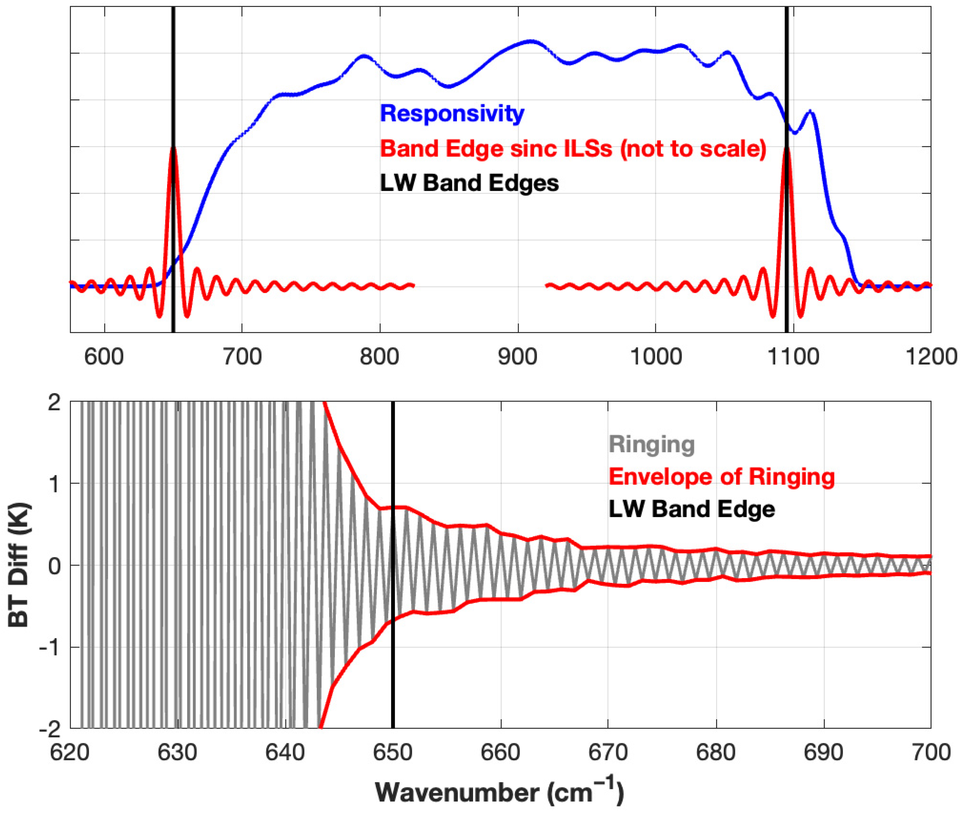
2. Characterization of CrIS Spectral Ringing Effects Using Calculated TOA Radiances

CrIS TOA radiances, S m , at channel center wavenumber, v m , are computed using:
S m ( v m ) = S R F ( v m v ) · R ( v ) · L ( v ) d v S R F ( v m v ) · R ( v ) d v S R F ( v m v ) · R ( v ) · L ( v ) d v R ( v m )
where L ( v ) is the monochromatic radiance at TOA, SRF is the CrIS SRF which, as discussed previously, is a pure sinc function, R ( v ) is the spectrally varying responsivity of the CrIS sensor, and the integrations are performed over all wavenumbers v. In this formulation, it should be noted, that R ( v ) varies smoothly in the spectral domain compared to the narrow sinc SRF, making the final formula a very accurate approximation. From Equation (1) we can see that the observed CrIS radiance spectrum is not simply L ( v ) convolved with the CrIS SRF. Radiometric and spectral components of the CrIS calibration remove various effects, but they do not remove the effect of the spectrally varying shape of the responsivity on the effective SRF. To most accurately calculate a CrIS spectrum which matches the calibrated CrIS spectrum, R ( v ) should be taken into account. This is in contrast to the typical methodology where instead of using the sensor responsivity shape, an artificial band-rolloff function, such as a cosine or exponential function, is used to smoothly taper the monochromatic spectrum to zero outside of the usable spectral range.
Here, we illustrate the theory using the actual CrIS sensor responsivity derived from views of the internal calibration target (ICT) and deep space (DS) views. Figure 1 provides an example of the CrIS responsivity for one of the CrIS S-NPP longwave detectors. Overlaid on the responsivity curve are scaled SRF sinc functions that show how an ideal FTS instrument weights nearby spectral points. The example SRFs are artificially broadened by an order of magnitude in the wavenumber axis so that the extended side-lobes of the unapodized sinc function can be seen. For CrIS, the ideal SRF (i.e., with self apodization effects removed) is a sinc function with a zero-crossing consistent with the CrIS wavenumber grid spacing of 0.625 cm−1. The sinc functions shown are centered at the CrIS user grid band edges. Note that at the band edge at 650 cm−1 the responsivity has a strongly wavenumber dependent slope.
At the longwave band edge at 650 cm−1, the symmetrical SRF function has relatively large signal contributions from the high wavenumber side and relatively low signal contributions from the low wavenumber side. The process of radiometric calibration removes the broad-band shape of the CrIS responsivity. However, if unaccounted for, this asymmetry creates spectral artifacts that are often referred to as ‘ringing’, because they alternate between small positive and negative biases for every other optimally sampled point. The figure also demonstrates that the ideal calibrated SRF has contributions well outside the user-band of CrIS including spectral regions where CrIS has negligible sensitivity. Thus, the standard calibration procedures cannot produce, for example, data for a channel centered at the LW band edge of 650 cm−1 with the advertised SRF of a pure sinc function with contributions from spectral regions where CrIS has no measured signal. Clearly, this actual responsivity will create spectral artifacts relative to the result with an ideal flat and unbounded responsivity.
The bottom panel of Figure 1 shows an example characterization of this effect. The ringing effect is shown for the spectral region around the LW band edge, where the ringing artifact is defined here as the difference between a typical earth spectrum calculated with FOV5 responsivity applied (Equation (1)) and a spectrum calculated with effectively infinite-band rolloffs and a flat responsivity. The back-and-forth nature of the ringing is evident along with the envelope of the ringing (red curves connecting every other spectral point, for both odd and even sets of points). Both the finite band extent and non-flat character of the realistic responsivity contribute to this ringing, and this high frequency effect is associated with the largest OPD signals of the interferograms.

2.1. Methodology for Including Spectral Ringing in Calculated TOA Radiances

The remainder of this section describes the calculation of the CrIS responsivities and the method used to account for responsivity-induced ringing in simulated CrIS radiances. The ringing impact from the finite-band sensitivity and non-flat in-band responsivities for CrIS are simulated in this section. The FOV and sensor (S-NPP versus NOAA-20) dependencies of the responsivities are also investigated.

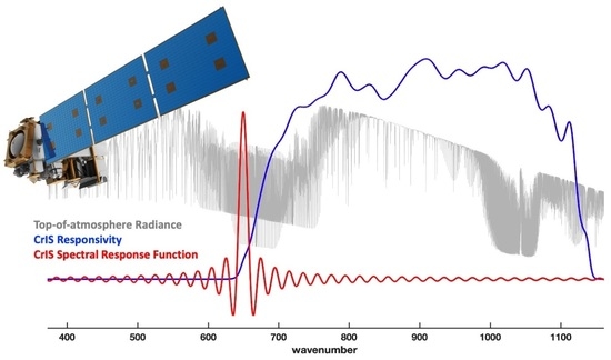
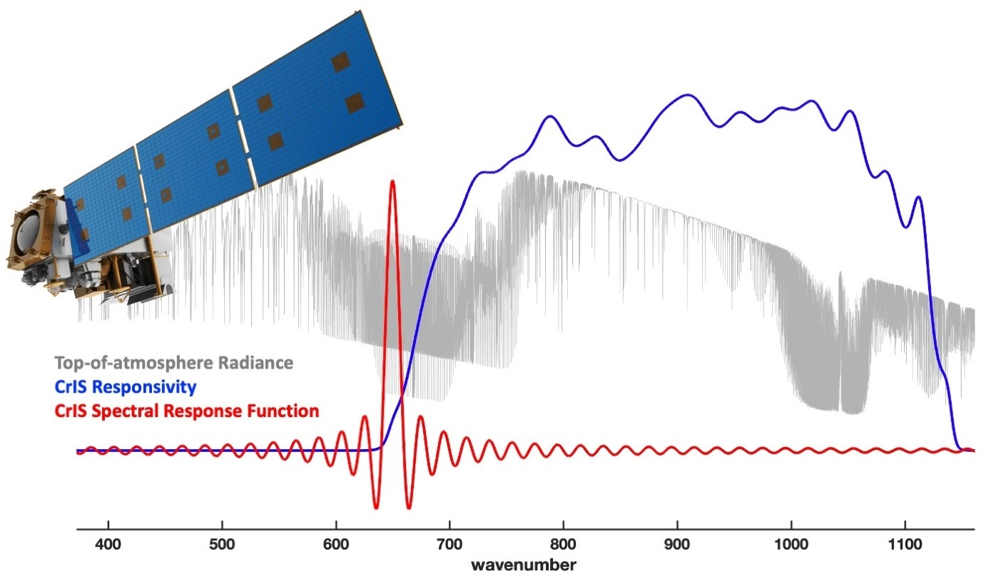
2.1.1. Sensor Responsivities

The spectral responsivity magnitudes, R ( v ) , used in this investigation are computed using:
R ( v ) = | C I C T ( v ) C D S ( v ) | B ( T I C T ) ( v )
where C I C T ( v ) and C D S ( v ) are complex spectra for in-orbit views of the CrIS calibration targets, including the Internal Calibration Target (ICT) which is an on-board blackbody and views of the near zero radiance Deep Space (DS). TICT is the effective temperature of the ICT and is approximately 285 K, and B represents the Planck function of blackbody radiance. Opposed to the actual calibration processing, exact modeling of the ICT and DS predicted view radiances is not required to compute representative responsivities for this application. Additionally, opposed to operational Normal Mode (NM) CrIS data, CICT and CDS used here are obtained from Diagnostic Mode (DM) data which is collected periodically for diagnostic purposes. The DM data by-passes the operational on-board Finite Impulse Response (FIR) filtering and decimation processing which is performed to reduce on-board data volume. As a result, the DM data contains information on the CrIS response for all wavenumbers from 0 cm−1 to the Nyquist frequency. It also does not contain the spectral shape of the FIR filtering and therefore represents the spectral content needed for this application. S-NPP CrIS R ( v ) values were computed using DM data collected on-orbit on 9 February 2012 from 13:09 to 23:45 UTC, and NOAA-20 R ( v ) values were computed using DM data collected on-orbit on 18 January 2018 12:33 to 19 January 2018 05:29 UTC. Interferogram sweep direction 0 data was used, although there is no significant difference if sweep direction 1 is used. Additionally, in the computation of the complex spectra C, artificial ‘rolloff’ functions were used to smoothly taper R ( v ) to zero in the out-of-band spectral regions, so that unwanted out-of-band contributions (due to, for example, interferogram double pass and nonlinearity) are not included in R ( v ) for this application. This was done where R ( v ) is close to zero (620–625 cm−1 and 1160–1165 cm−1 for the LW band, 1125–1130 cm−1 and 1820–1830 cm−1 for the MW band, and 2040–2050 cm−1 and 2650–2660 cm−1 for the SW band).
The on-orbit derived sensor responsivities for S-NPP and NOAA-20 CrIS are shown in Figure 2. These values are normalized to 1 at mid-band wavenumbers for each FOV so the shape of the responsivities can be compared. For S-NPP (right column) there is relatively small variation in R ( v )   among FOVs. For NOAA-20 (left column), the responsivities are somewhat different from the S-NPP shapes particularly for the LW band, and there is also more spread among FOVs in the LW. These variations are due to detector-to-detector property differences resulting from selecting for improved response at the longwave end. In terms of the effects on spectral ringing, and modification of the original information content of the measurements, note that the responsivities show significant non-flatness (versus wavenumber) particularly in the LW band, and that the spectral variations differ between S-NPP and NOAA-20. Also note that, particularly for the LW band, the slope of R ( v ) is very large near the LW end of the band and goes to zero very close to 650 cm−1 which is the beginning of the user-grid for the LW band. It should also be noted that the spectral shapes of the CrIS responsivities do not change significantly with time.

2.1.2. Monochromatic TOA Radiance Calculations

Equation (1) requires the computation of the top of atmosphere Radiance L ( v ) at very high spectral resolution, and here we use a monochromatic line-by-line model. Details of which particular model to use or the various inputs to the model are not central to the topic of this paper. However, accurate TOA radiance calculations are needed in order to make meaningful comparisons with the CrIS observations, and details of the calculations are described in Section 3.

2.1.3. Simulation of CrIS Radiances

Following Equation (1), the simulation of the CrIS radiances including the responsivity-induced spectral ringing undergoes the following list of steps. As a general overview, the responsivity is applied before transforming the radiances from monochromatic resolution to CrIS resolution and is subsequently divided out after resolution reduction. This mimics what happens in the measurement process followed by calibration.
  • Compute monochromatic upwelling infrared radiances for the altitude and satellite zenith angle of the sensor.
  • Linearly interpolate the monochromatic radiance spectra to a constant wavenumber grid equal to the final CrIS user grid interval divided by 2N where N is such that the interpolation wavenumber interval is less than the monochromatic grid interval.
  • Multiply the monochromatic radiances by the appropriate CrIS responsivity.
  • Perform a discrete Fourier transform to the interferogram domain.
  • Truncate the interferogram at the index corresponding to the CrIS maximum optical path difference, e.g., 0.8 cm for Full Spectral Resolution.
  • Perform the inverse Fourier transform (including the normalization factor N).
  • Divide out the CrIS responsivity at the CrIS user grid wavenumber scale.
  • Extract out the portion of the spectrum that corresponds to the CrIS spectral band limits (LW, MW, and SW).
By following this process, the calculated radiance, like the observed radiance, includes the ringing induced by the non-flat responsivity such that it is removed from Obs-Calc differences and does not get falsely interpreted as an atmospheric signal.
To characterize the effects of this new concept of including the sensor response in the calculated radiance, we compare to calculated radiances which do not incorporate the responsivity. Typically, when computing CrIS radiances using a line-by-line model, or in the creation of a parameterized fast-model such as the Community Radiative Transfer Model (CRTM) [10] or Radiative Transfer for TOVS (RTTOVs) [11], the shape of the CrIS responsivity is not considered; rather artificial roll-off functions are used to condition the input monochromatic radiance calculations outside the spectral regions of interest before the Fourier transform is performed. Practically speaking, the same steps as outlined above are followed except artificial rolloffs (for example exponential decay functions or half-cosine functions) are used in place of the CrIS responsivity.
In this paper two different sets of artificial rolloffs are used, each for different purposes–one is referred to as ‘infinite-bandwidth’ rolloffs and the other is referred to as ‘band-edge’ rolloffs. The ‘infinite-bandwidth’ rolloffs represent the theoretical limit of no band-pass limitations. While it is not feasible or practical to compute monochromatic radiances across the infinite spectrum to simulate the lack of band pass limitations, a very good approximation can be made by rolling off the calculations at a distance far away from the band edge. For this type of rolloff the bandpass half-cosine function is defined to begin rolling off at 100 cm−1 away from the CrIS user grid and goes to zero at 125 cm−1 away from the CrIS user grid. The other type of rolloff, ‘band-edge rolloffs’, are used to represent what most general users or fast models use in their simulation of CrIS radiances and here are defined to have the rolloffs that go to zero at the same spectral location where the CrIS responsivities go to zero. These artificial rolloff functions are shown in the top panel of Figure 3.
The difference between CrIS simulated radiances including the responsivities, and those computed without the responsivity and using an infinite-bandwidth rolloff is what we define as ‘true ringing’. The term ‘true’ is used because it is due to the original information content of the observations, and to differentiate it from other sources of spectral ringing. The following results include comparisons of clear sky CrIS spectra with calculated spectra computed with both approaches, with and without ‘true ringing’ included.
Finally, it should be noted that the incorporation of the sensor responsivity to condition the input monochromatic spectrum does not introduce any significant computational expense. Whether in the creation of a parameterized fast model or individual calculations using a line-by-line model, some type of rolloff function is needed, and using the responsivity instead of an empirical function is a negligible computational cost.

2.2. Results

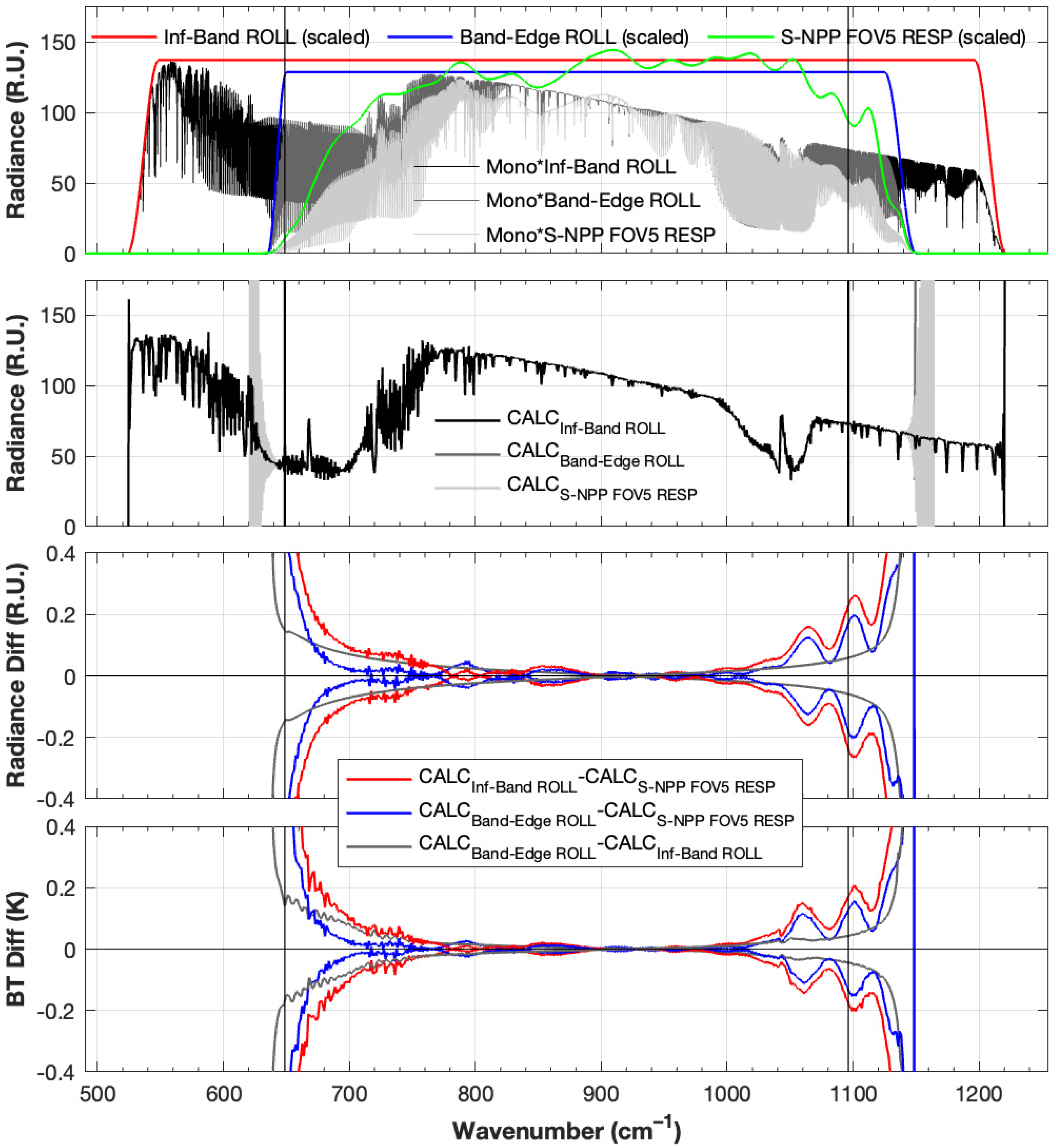
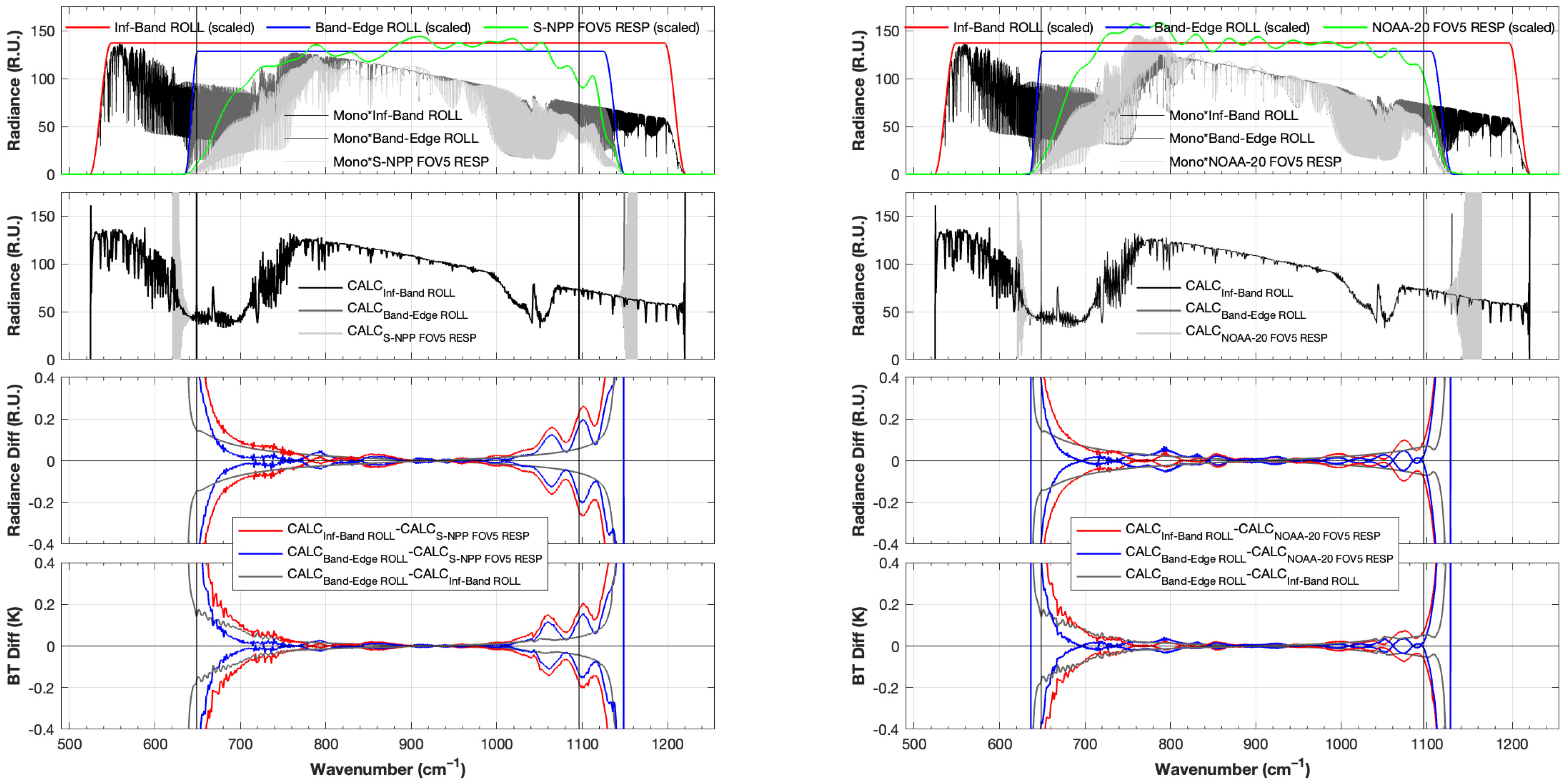
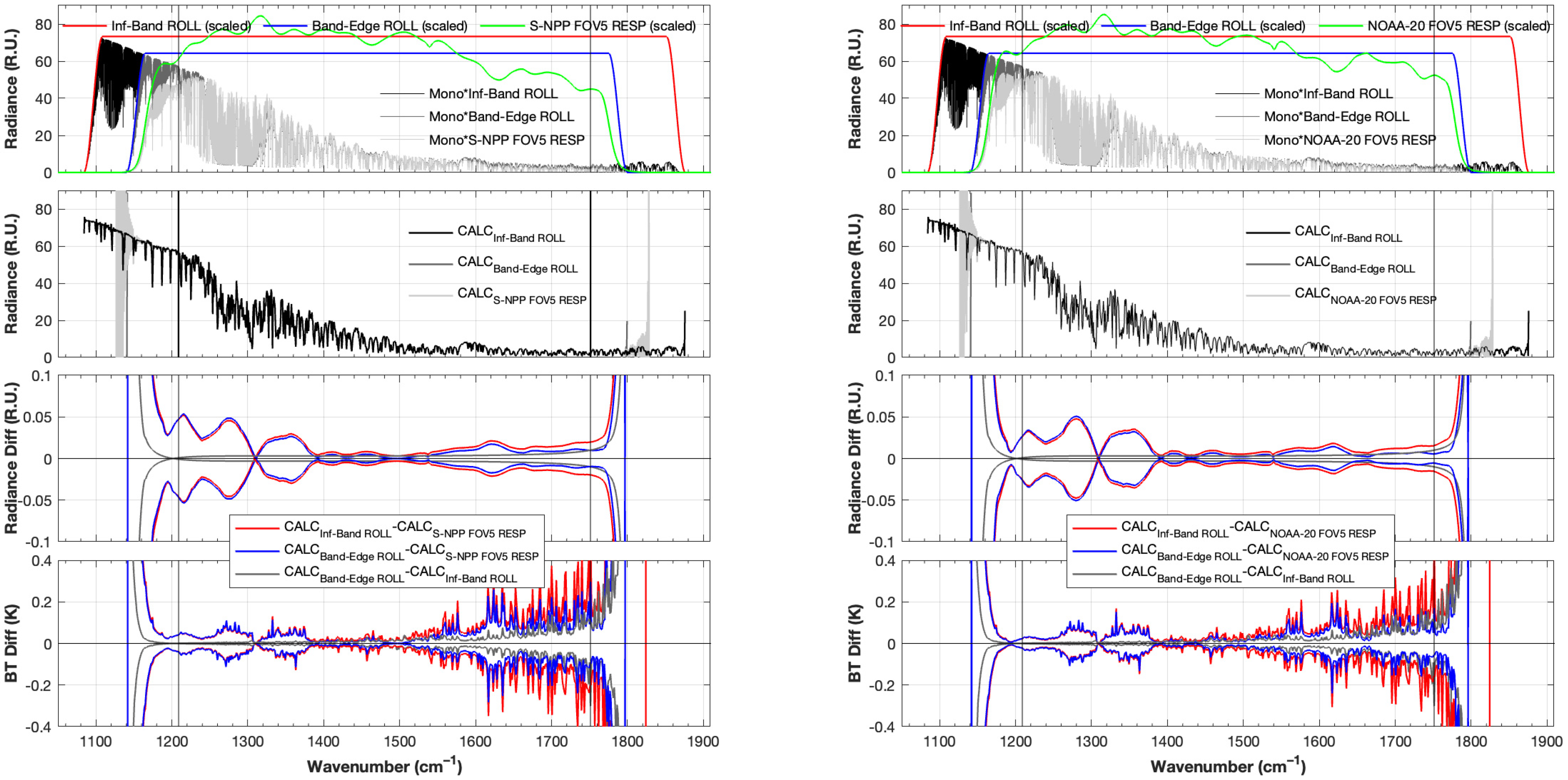
2.2.1. Impact of Responsivities versus Artificial Rolloffs on Calculations

Figure 3 illustrates the impact of using responsivities versus rolloffs on calculations and the nature of S-NPP ringing for the LW band. Similar figures for both S-NPP and NOAA-20 and for all three spectral bands are included in Appendix A. This is done using an example calculated clear sky TOA spectrum. The top panel of each of these figures shows the calculated monochromatic spectra multiplied by the infinite-band rolloffs (black), the band-edge rolloffs (dark gray), and FOV5 responsivity (light gray). These are overlaid with the scaled rolloffs (red and blue) and responsivity (green). The second panel shows the CrIS Full Spectral Resolution (FSR) radiances, which are the output from Step-8 outlined above in Section 2.1.3 for the cases with the infinite-band rolloffs, band-edge rolloffs, and FOV5 responsivity applied. The bottom two panels show the envelope of the ringing in radiance units (third panel from top) and in brightness temperature (bottom panel). The ringing is defined as the difference between the calculations with the rolloffs applied and the calculations with the FOV5 responsivity applied, with infinite-band rolloffs (red) and band-edge rolloffs (blue). Also shown is the difference between the infinite-band rolloff result and the band-edge rolloff result (gray). From the previous discussion, the red curve therefore characterizes the effects due to both in-band non-flatness of the responsivity and finite spectral extent of the responsivity, the blue curve characterizes mainly the effect due only to in-band non-flatness, and the gray characterizes mainly the effect due only to finite spectral extent. Note that near the beginning of the LW band (where the responsivity is already small) the impact of finite out-of-band sensitivity (gray, or red minus blue) is substantially larger than the effect caused by the non-flat responsivity (blue). As shown in the appendix, S-NPP and NOAA-20 have similar instrument ringing characteristics across the bands. Ringing effects are relatively small throughout most of the spectrum (< +/−0.1 K), with the largest ringing effects at the longwave end of the longwave band reaching approximately +/−0.5 K, at the shortwave side of the MW band reaching about +/−0.4 K, and in the SW CO2 band reaching about +/−0.2 K.

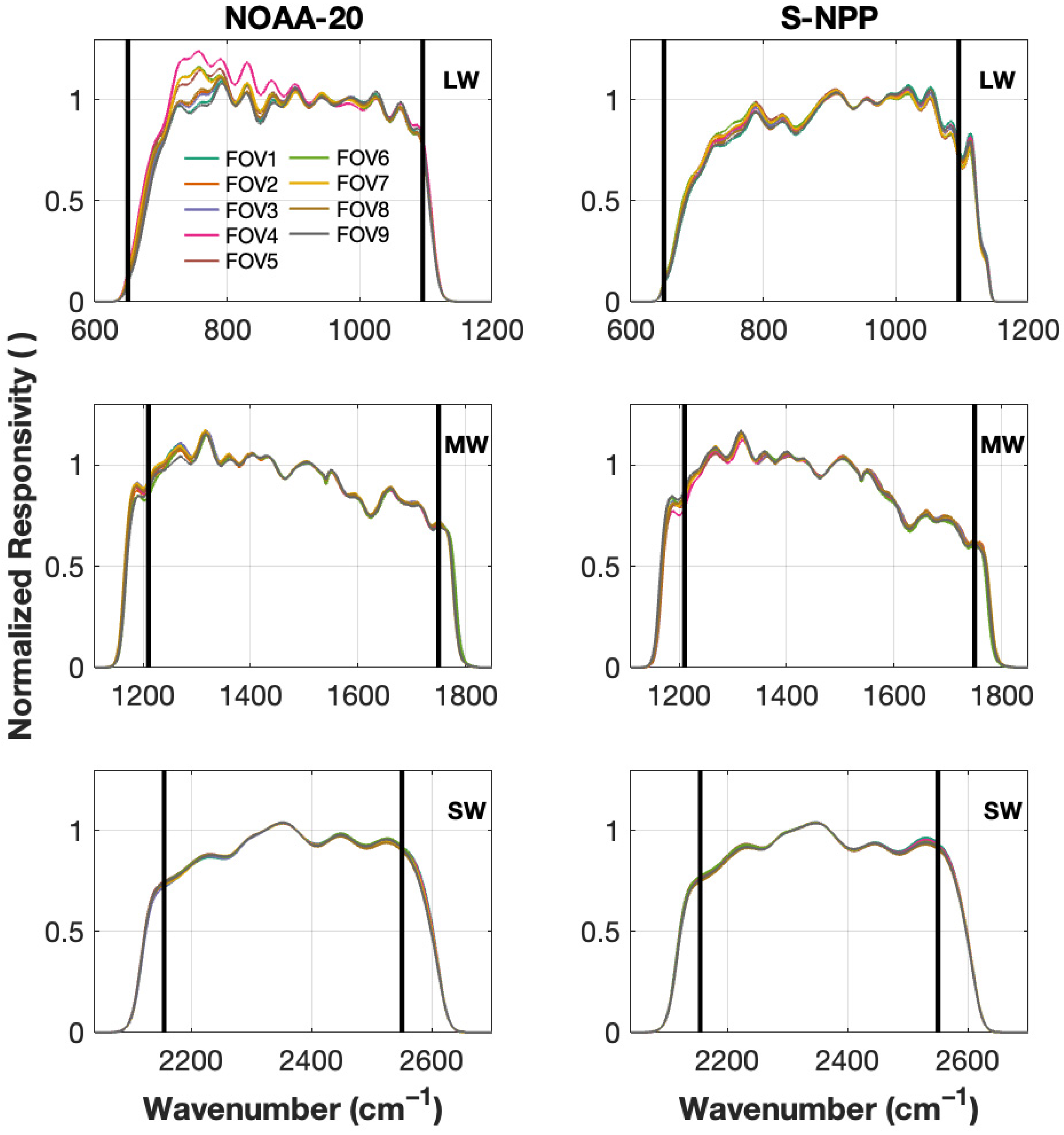
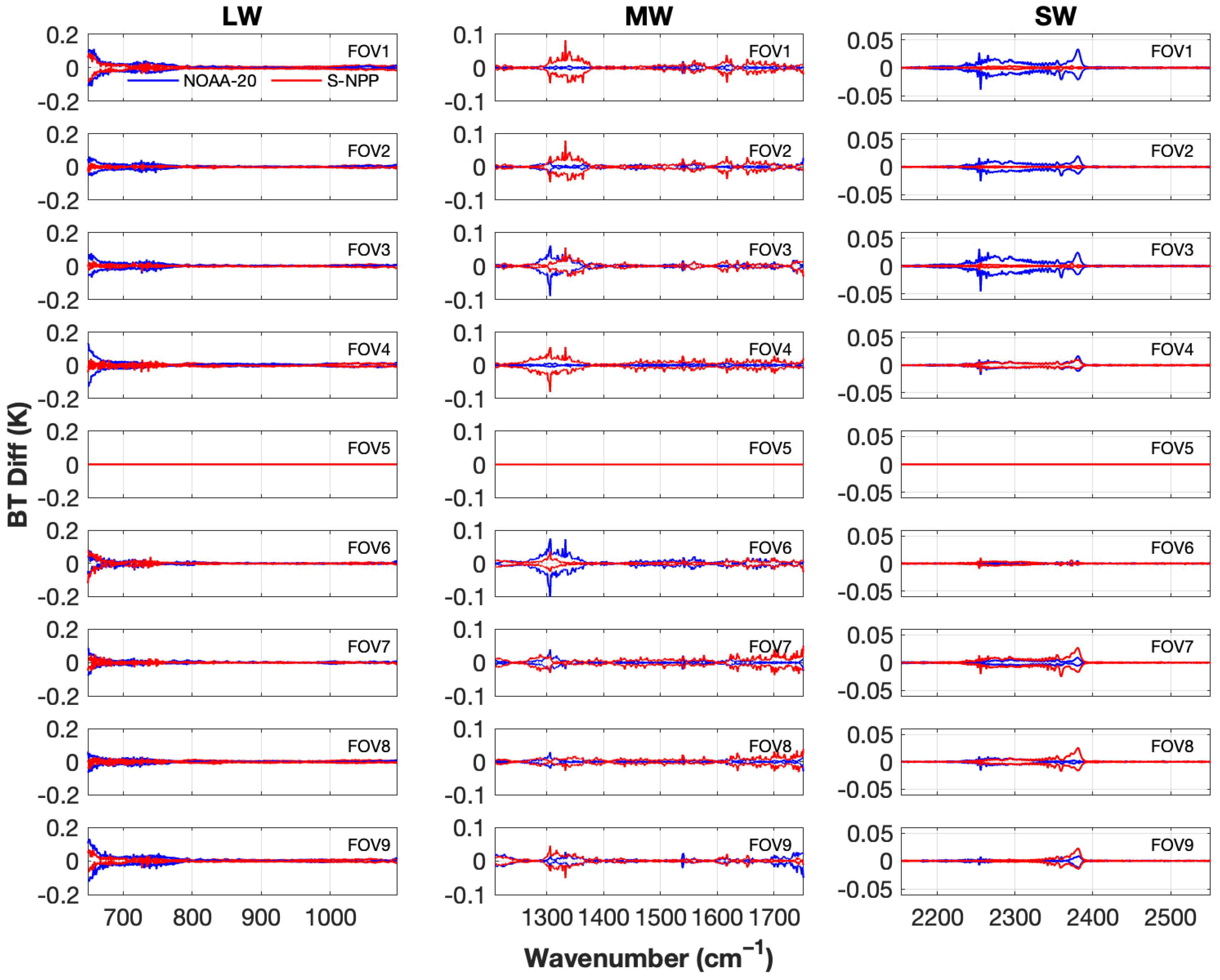
2.2.2. FOV and Sensor Dependence of Responsivities

As shown in Figure 2 there are small differences in the shape of the responsivity for each of the nine FOVs and differences between the S-NPP and NOAA-20 responsivities. The effect of using FOV dependent responsivities to calculate CrIS radiances, versus using a single responsivity for all FOVs, is shown in Figure 4 for both NOAA-20 (blue) and S-NPP (red). All panels show the envelope of the difference of the monochromatic calculation with the FOV X responsivity applied from the monochromatic calculation with FOV5 responsivity applied, where X is each of the FOVs 1–9. This is shown for each band; LW (left), MW (center), and SW (right) and for each FOV with FOV1 in the top-panel through to FOV9 in the bottom-panel. In general, the differences are small, compared to the overall ringing effects shown in Figure 3 and similar figures in Appendix A. Even the largest differences at the longwave end of the longwave band are only about +/−0.1 K. These results provide important information for a determination if calculations can be performed with a single responsivity curve for all CrIS data, or if FOV and sensor specific responsivities should be used. For most applications, the FOV and sensor dependency can be ignored, for the S-NPP and NOAA-20 sensors.

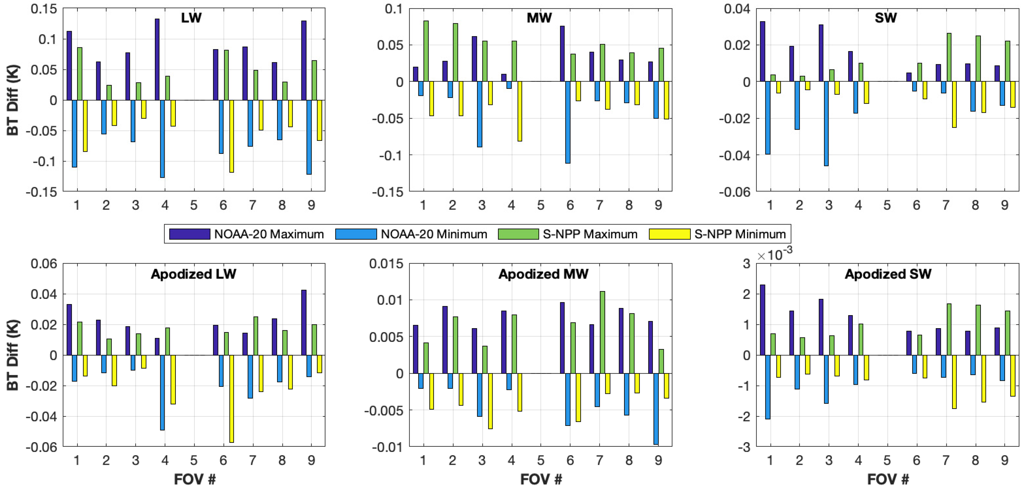
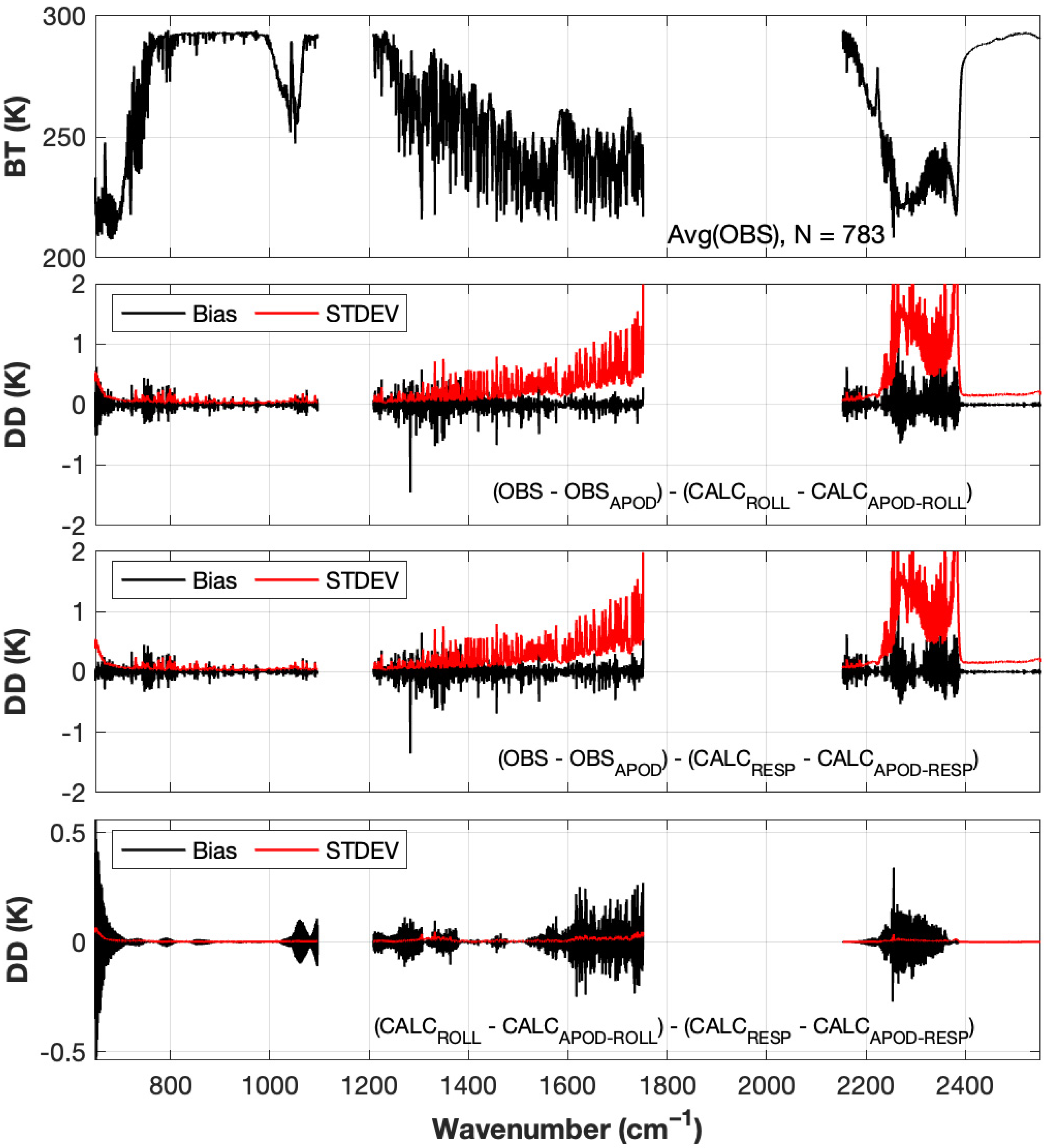
2.2.3. Effects of Hamming Apodization

Results shown in Figure 3 and Figure 4 are for unapodized CrIS data with a pure sinc SRF. To simulate apodized CrIS spectra, the prescription given in the CrIS SDR ATBD [3] (pp. 79–82) is used, specifically a Hamming apodization function with a Hamming parameter of a = 0.23. These apodized spectra are of interest to this study as they are representative of how CrIS data are currently being used by NWP centers [12]. Hamming apodization results in a strong spectral smoothing, and spectral correlation, of signal and noise of the unapodized spectra, and thus greatly reduces the every-other-point ringing effects. For example, the ringing effects shown in Figure 3 are reduced by a factor of approximately 5 for Hamming apodized spectra. However, for CrIS, Hamming apodization is not a good solution to remove ringing, because it also greatly reduces the high spectral resolution information content from the key 15 micron carbon dioxide band.
To illustrate the effect of using FOV dependent responsivities with apodized calculations, the maximum and minimum differences for each FOV are shown in the bar graphs in Figure 5. The top row shows the maximum and minimum differences for the unapodized calculations, for the same calculations shown in Figure 4, and the bottom row for apodized versions of these calculations for the LW (left), MW (center), and SW (right) bands. Along with the overall reduction in ringing effects when Hamming apodization is applied, the FOV dependencies are also reduced by a factor of approximately 5 when Hamming is applied, with maximum brightness temperature differences of several hundredths Kelvin.
Also, while the responsivity effect on spectral ringing is much less apparent when working with Hamming apodized spectra, it should be recognized, that Hamming apodization is completely reversible in the interferogram or spectral domain if adjacent spectral channels are retained. So, the apparent reduction in ringing effects for Hamming apodized spectra is also reversed if the full unapodized spectral content is retained in an application using Hamming apodized data. For example, it has been proven that rigorous optimum estimation retrievals of apodized spectra effectively remove the apodization when all spectral channels are retained, and the noise covariance specified properly includes the correlated noise created by apodization [13].

3. Comparisons of Observed and Calculated Clear Sky Radiances

Section 2 demonstrated the CrIS responsivity effect on TOA calculated radiances. In this section we show comparisons of clear sky observed and calculated CrIS spectra, with and without the responsivity taken into account. This includes a description of the specific CrIS data used, details of the TOA calculations including the line-by-line radiative transfer model and its inputs, and results. These results are included to show the overall impact of incorporating the responsivity into the calculated radiances. In some spectral regions, where there is good agreement between observed and calculated spectra, there are obvious improvements when including the responsivity, while for other spectral regions the comparisons are affected by various factors and the improvements are not apparent.

3.1. Infrared Observations

The infrared observations used in this study are from Suomi-NPP CrIS on 20 January 2016 between 03:06:38 and 03:12:32 UTC. The full spectral resolution (FSR) radiances were produced offline at NOAA STAR using the current operational SDR algorithm as described in Han and Chen [9]. The exact same granule files as used in Han and Chen [9] were selected for consistency, however any CrIS granule at the same latitude would produce similar results.
Radiance calculations are performed for nighttime (corresponding to solar zenith angles greater than 96 degrees), clear sky scenes over the ocean. Additionally, to screen out view angles larger than ~35 degrees, only fields of regard 6–25 are used. A spatial uniformity test is used to restrict the clear FOVs to be only those whose FORs have a 900 cm−1 observed BT standard deviation less than or equal to 0.25 K. Additionally, the 900 cm−1 BT must be within 2 K of the ERA-Interim skin temperature which is interpolated in space and time to the CrIS footprint. Lastly, to maintain the same number of samples for each of the 9 CrIS detectors, the 3 × 3 arrays of fields of view are maintained, i.e., it is required that all 9 FOVs within a given FOR pass the scene selection in order that any be kept for analysis.

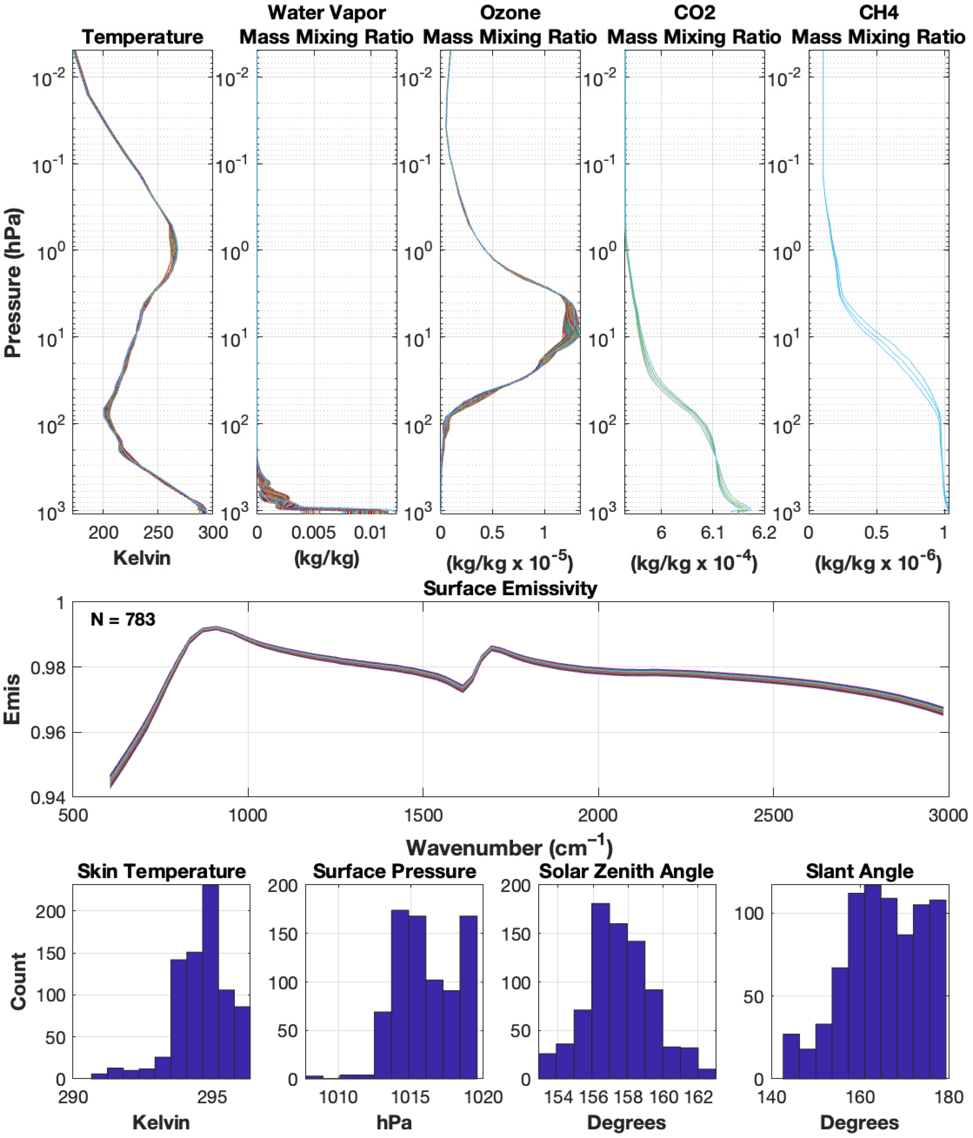
3.2. Monochromatic Radiance Calculations

For the monochromatic radiance calculations, the Atmospheric and Environmental Research Line-by-Line Radiative Transfer Model (LBLRTM) double precision version 12.6 is used [14]. The line parameter database used in conjunction with the model is ‘aer_v_3.5′ and is based off of the HITRAN 2012 database [15] with updates made to the CO2, H2O, CH4, and O2 line parameters [16,17,18,19]. Input to LBLRTM includes atmospheric state and model parameters which vary for each radiance calculation. Atmospheric model data from the ERA-Interim reanalysis [20,21] is bilinearly interpolated to the time of the measurement and the location of the FOV’s corresponding field of regard latitude and longitude, which is based on the FOV 5 location. Since the ERA-Interim does not report profile values up to the top of the LBLRTM model grid, AFGL climatology lapse rates are used to extrapolate the ERA-Interim profiles. The day of year and latitude determines which AFGL model atmosphere is used for interpolation. Before being input to the model, these atmospheric profiles are interpolated to a fixed 101 pressure level grid and then modified so that the surface value has an equivalent pressure to that defined by the input surface pressure. Carbon dioxide and methane data from NOAA’s CarbonTracker [22] are also used; monthly, zonally averaged profiles are computed for input into the model. Heavy molecule profiles—those of CCl3F (F11), CCl2F2 (F12), and CCl4 are scaled so the surface values are equivalent to current day values obtained from NOAA Earth System Research Laboratories (ESRL). Surface emissivity is determined using an ocean emissivity look-up-table which is dependent upon surface wind speed and the CrIS view angle [23,24]. The CrIS view angle is also used in the calculation of the radiance.
NOAA’s ESRL CarbonTracker is used to define atmospheric carbon dioxide and methane. Data can be found online at http://carbontracker.noaa.gov (accessed on 23 October 2022) and more information in Peters, W. et al. [22]. ECMWF’s ERA-Interim reanalysis model (http://www.ecmwf.int/en/research/climate-reanalysis/era-interim, accessed on 27 October 2022) [20,21] is used to obtain atmospheric temperature, water vapor, and ozone profiles, in addition to skin temperature, surface wind speed, and surface pressure. The ERA output provides global grids at 6 hourly increments. The 0.75° gridded, model level product is used, which reports output up to vertical pressure levels of ~0.1 hPa. This corresponds to a horizontal resolution of ~80 km. An ocean emissivity look-up-table, which was provided by Nick Nalli [23,24,25], is used to define surface emissivity. The look-up-table uses the Cox and Munk [26] wave slope probability distribution function, a salinity correction, and the Hale and Querry [27] pure water refractive indices. The Air Force Geophysics Laboratory (AFGL) Atmospheric Constituent Profiles [28] are used as a background climatology in this study. Ozone, temperature, and water vapor profiles are used. Figure 6 shows the LBLRTM input profiles and histograms for various atmospheric state and surface parameters.

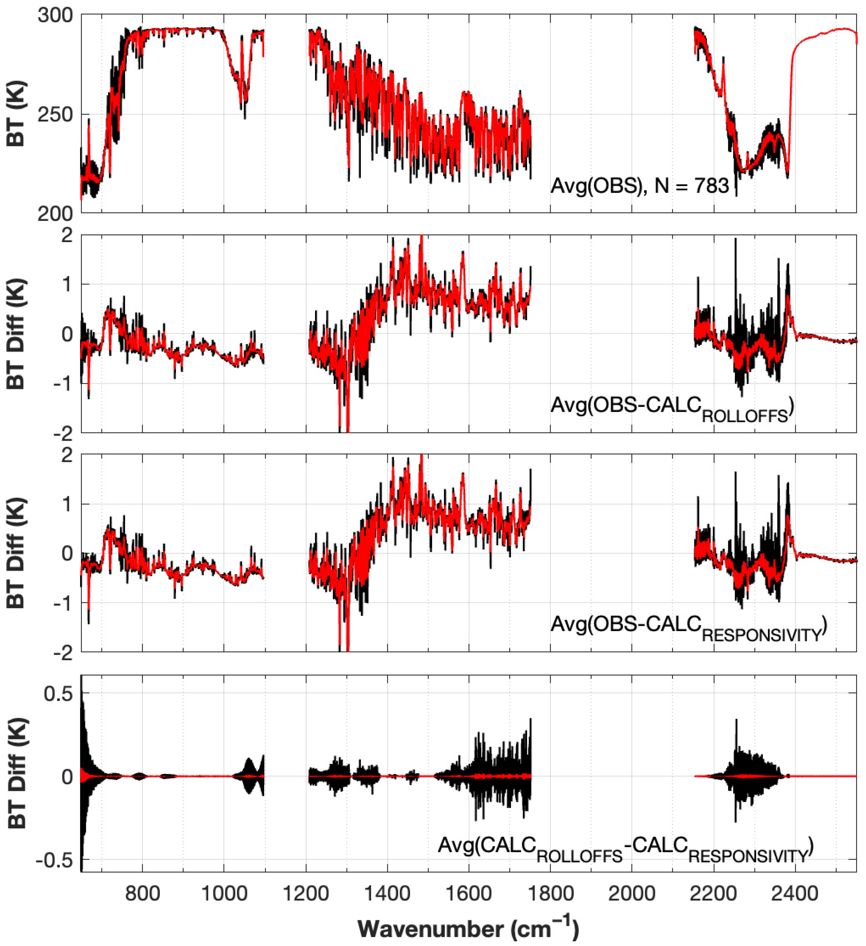
3.3. Impact on Observations—Calculations Differences

The impact of including the CrIS responsivity in calculated TOA radiances (i.e., Equation (1)) when comparing to clear sky observed CrIS radiances is shown in Figure 7. As in Section 2, calculations using the responsivity and calculations using infinite-band rolloffs are used, to characterize the effects and show the improved agreement when using the responsivity. This is for a clear-sky scene consisting of 783 clear sky footprints on 20 January 2016 at ~3:10 UTC. Results are shown for both unapodized (black) and Hamming apodized (red) spectra. The top panels show the all-FOV average of the 783 CrIS observations. The second panels from the top show the difference of the calculations with infinite-bandwidth rolloffs applied from the observations. The third panels show the differences of the calculations with FOV dependent responsivities applied from the observations. The bottom panels are the differences of the two previous panels and are estimates of the ringing. Overall, the ringing effects are generally smaller than other sources of differences, such as specification of the surface or atmospheric state or systematic errors in the line-by-line model. However, at the LW end of the LW band, the ringing effects are considerably large with respect to the total observed residual, with improved agreement when the responsivities are included compared to the typical approach, highlighting the potential importance of recognizing and handling this effect. For the Hamming apodized results, the ringing effect is an order of magnitude lower when the apodization is applied, but again note that this is somewhat of an artificial result. If an application uses the full spectral information, the Hamming apodization is reversed and the unapodized spectral ringing effect is retained. Also note the detrimental effect of apodization on the high spectral resolution signature of carbon dioxide in the region from 700 to 790 cm−1.
Artifacts related to data apodization are further explored using a double difference (DD) method where the Hamming apodization is applied to both observations (Obs) and calculations (Calc):
D D = [ O b s H a m m i n g ( O b s ) ] [ C a l c H a m m i n g ( C a l c ) ]
where the calculation is conditioned with the detector responsivity (i.e., Equation (1)). This technique removes the larger and more slowly varying spectral features which are caused by errors in the input atmosphere into the RTM or by radiometric effects. It should be stressed that this quantity will also include spectral features which are not due to ‘true’ ringing (i.e., radiometric features associated with lower OPDs), but it does clearly separate out some of the main ringing features identified in Section 2. This double difference technique was introduced and discussed by Strow et al., [8] to characterize the ‘excessive ringing’ of the S-NPP CrIS instrument. In that study, excessive ringing associated with an initial, at-launch problem with the FIR filter was seen in S-NPP CrIS, but this problem was quickly resolved and should not be considered normal behavior for the S-NPP instrument. In this paper, the term excessive ringing should not be confused with the term true ringing.
Figure 8 uses this double difference method to estimate the ringing residual for the same clear-sky scene described in Figure 7. Similarly, the top panel shows the all FOV average of the CrIS unapodized observations for this case-study. The bias (black) and standard deviation (red) between the unapodized and apodized observations and unapodized and apodized calculations (Equation (3)) with rolloffs applied are shown in the second panel and with FOV dependent responsivities applied in the third panel. The ringing residual is shown in the bottom panel and is the difference between the second and third panels. Using this technique more clearly highlights the spectral ringing effects, including most importantly the improved agreement between observed and calculated spectra at the LW end of the LW band when the CrIS responsivity is included.

4. Discussion

This paper has introduced the concept of including the CrIS spectral responsivity when computing CrIS TOA radiances. Spectral variations in optical transmission and detector response can interact with the non-local sinc SRF of an FTS instrument. Comparisons to radiances computed using typical artificial rolloff functions are shown to characterize the impact of using the responsivities. The differences are described as spectral ringing and are associated with high frequency oscillations of every-other minimally sampled spectral channel. The comparisons quantify the total effect of using the responsivity as well as separating out what is due to the finite spectral extent of the CrIS responsivity and what is due to the spectral non-flatness of the in-band responsivity.
The magnitude of spectral ringing is seen to be similar in size for each of the three spectral bands, as shown in Figure 3, Figure A1, Figure A2 and Figure A3. In brightness temperature units the effects are small for large portions of the spectrum but as large as +/−0.5 K. The most pronounced effect is found at the longwave end of the LW band, where the edge of the user band at 650 cm−1 is close to where the sensor responsivity goes to zero at approximately 640 cm−1 and where the spectral gradient of the responsivity is large. Calculations demonstrating the ringing differences of the responsivities for each of the nine FOVs and for two CrIS instruments (S-NPP and NOAA-20) were also shown. The S-NPP and the NOAA-20 CrIS instruments have similar ringing characteristics. The FOV dependence is small, on the order of +/−0.15 K, +/−0.1 K, and +/−0.05 K for the LW, MW, and SW bands, respectively, as shown in Figure 4.
These results suggest that for many applications the individual detector variations among the nine FOVs in each band can be safely neglected in the simulation of S-NPP and NOAA-20 CrIS sensors. Instead, an average responsivity, or the FOV 5 values, can be used in each CrIS band in the simulation of CrIS sensors. To most accurately model the observed CrIS SDR spectra in terms of spectral ringing behavior, this approach is recommended over the typical approach of using artificial rolloff functions, for the conditioning of monochromatic radiance calculations, or in the production of a CrIS fast radiative transfer model.
The impact of the responsivity/ringing effect was also shown in terms of comparisons of clear sky observed and calculated spectra. Calculations which incorporate the sensor responsivities show better agreement with the observations, most notably at the longwave end of the LW band. Figure 7 shows that the magnitude of the responsivity ringing effect is relatively small compared to the typical difference between observations and calculations. However, Figure 7 and Figure 8 also show that the ringing contribution due to responsivity spectral variations can be systematic in nature and does not average to zero in a statistical dataset of CrIS observations. This is seen in the bottom panel of Figure 8 which shows that the standard deviation of the differences over this dataset are much smaller than the mean difference spectrum. It is important to note, however, that this particular result is derived from an ensemble of spectra with low variability. The ringing artifacts are not a pure static bias for all possible spectra. Rather the artifacts are scene dependent and cannot be easily removed with standard bias correction schemes.
The effect of Hamming apodization was also shown in Figure 5 and Figure 7 and discussed. Having a strong spectral smoothing effect, Hamming apodization greatly suppresses the high frequency spectral ringing behavior, reducing the effects in brightness temperature by roughly a factor of 5 below the unapodized results, to apparently negligibly small values. The authors, however, stress that if the applications of Hamming apodized CrIS data are designed to make full use of the CrIS spectral information content, then the full unapodized spectral information is retained, along with the unapodized spectral ringing effects.
Future work includes further development and demonstration of a new ground processing calibration module which will remove the effects of the responsivity on the effective SRF of the CrIS calibrated radiances. This technique involves modification of the calibrated interferogram values for large OPD values near the ends of the interferograms and is beyond the scope of this paper. This approach would avoid the need to include sensor specific responsivity information in radiative transfer models.

5. Conclusions

This paper has provided a procedure for the simulation of CrIS radiances to include spectral ringing effects caused by the finite-band, non-flat instrument spectral response to incident radiation. Simulations have been performed to illustrate the magnitude of the effects and to indicate which spectral channels are impacted. Comparisons of calculated spectra with CrIS observations show that for most channels this effect is negligibly small compared to errors in the radiative transfer calculations but for the longwave edge of the CrIS longwave band and a few other regions, the brightness temperature ringing is significant. While the ringing artifact described in this paper may appear to be removed when Hamming apodization is applied, it is still present, and its influence reappears if the spectral correlation induced by apodization is properly handled to preserve the information content that derives from high spectral resolution. Inclusion of the instrument responsivity in calculated spectra to properly mimic the observed spectra as defined here eliminates artifacts from this type of ringing. Users should consider whether this effect is important for their particular application. Future work involves performing a correction for the ringing effects as part of the CrIS calibration process.

Author Contributions

Conceptualization, H.R., J.T., Y.C. and D.T.; Formal analysis, L.B., M.L. and D.T.; Project administration, F.I.-S. and D.T.; Visualization, L.B. and M.L.; Writing—original draft, L.B., M.L., R.K., H.R. and D.T.; Writing—review and editing, L.B., M.L., R.K., H.R., J.T., Y.C., F.I.-S. and D.T. All authors have read and agreed to the published version of the manuscript.

Funding

This researched was supported by NOAA NESDIS, grant NA20NES4320003.

Data Availability Statement

Data used in this study is described in detail in Section 3.1 and Section 3.2.

Acknowledgments

We would like to thank Rolf Stuhlmann for initial discussion on this topic, as well as helpful discussions with Dorothee Coppens, Bertrand Theodore, and Pierre Dussarrat.

Conflicts of Interest

The authors declare no conflict of interest. The scientific results and conclusions, as well as any views or opinions expressed herein, are those of the author(s) and do not necessarily reflect those of NOAA or the Department of Commerce.

Appendix A

Figure A1. Calculated ringing effects for S-NPP (left) and NOAA20 (right) for an example clear sky spectrum in the LW band. Monochromatic calculated spectrum multiplied by infinite-band and band-edge rolloffs and CrIS FOV5 responsivity overlaid by scaled rolloffs and FOV5 responsivity (top panel); CrIS FSR resolution spectra with infinite-band and band-edge rolloffs and responsivity applied (second from top panel); envelope of the ringing, defined as the difference between the calculations with the rolloffs applied and the calculations with the responsivity applied, in radiance units (third panel from top) and in brightness temperature (bottom panel).
Remotesensing 15 00334 g0a1
Figure A2. Same as previous but for the MW band.
Remotesensing 15 00334 g0a2
Figure A3. Same as previous but for the SW band.
Remotesensing 15 00334 g0a3

References

  1. Han, Y.; Revercomb, H.; Cromp, M.; Gu, D.; Johnson, D.; Mooney, D.; Scott, D.; Strow, L.; Bingham, G.; Borg, L.; et al. Suomi NPP CrIS measurements, sensor data record algorithm, calibration and validation activities, and record data quality. J. Geophys. Res. Atmos. 2013, 118, 12734–12748. [Google Scholar] [CrossRef]
  2. Goldberg, M.D.; Kilcoyne, H.; Cikanek, H.; Mehta, A. Joint Polar Satellite System: The United States next generation civilian polar-orbiting environmental satellite system. J. Geophys. Res. Atmos. 2013, 118, 13463–13475. [Google Scholar] [CrossRef]
  3. STAR JPSS Science Documents. Joint Polar Satellite System (JPSS) Cross Track Infrared Sounder (CrIS) Sensor Data Records (SDR) Algorithm Theoretical Basis Document (ATBD) for Full Spectral Resolution, Document D0001-M01-S01-002_JPSS_ATBD_CrIS-SDR_fsr_20180614, June 2018. Available online: https://www.star.nesdis.noaa.gov/jpss/documents/ATBD/D0001-M01-S01-002_JPSS_ATBD_CRIS-SDR_fsr_20180614.pdf (accessed on 23 November 2022).
  4. Taylor, J.; Revercomb, H.; Tobin, C. An analysis and correction of polarization induced calibration errors for the cross-track infrared sounder (CrIS). In Sensor, Light, Energy and the Environment (E2, FTS, HISE, SOLAR, SSL); Paper FW2B.3; OSA Technical Digest (Optical Society of America): Washington, DC, USA, 2018. [Google Scholar] [CrossRef]
  5. Taylor, J.; Revercomb, H.; Tobin, D.; Knuteson, R.; Loveless, M.; Malloy, R.; Suwinsky, L.; Iturbide-Snachez, F.; Chen, Y.; White, G.; et al. Assessment and Correction of View Angle Dependent Radiometric Modulation due to Polarization for the Cross-track Infrared Sounder (CrIS). Remote Sens. 2022. submitted for publication. [Google Scholar]
  6. Zavyalov, V.; Esplin, M.; Scott, D.; Esplin, B.; Bingham, G.; Hoffman, E.; Lietzke, C.; Predina, J.; Frain, R.; Suwinski, L.; et al. Noise performance of the CrIS instrument. J. Geophys. Res. Atmos. 2013, 118, 13108–13120. [Google Scholar] [CrossRef] [Green Version]
  7. Tobin, D.; Revercomb, H.; Knuteson, R.; Taylor, J.; Best, F.; Borg, L.; DeSlover, D.; Martin, G.; Buijs, H.; Esplin, M.; et al. Suomi-NPP CrIS radiometric calibration uncertainty. J. Geophys. Res. Atmos. 2013, 118, 10589–10600. [Google Scholar] [CrossRef]
  8. Strow, L.L.; Motteler, H.; Tobin, D.; Revercomb, H.; Hannon, S.; Buijs, H.; Predina, J.; Suwinski, L.; Glumb, R. Spectral calibration and validation of the Cross-track Infrared Sounder on the Suomi NPP satellite. J. Geophys. Res. Atmos. 2013, 118, 12486–12496. [Google Scholar] [CrossRef]
  9. Han, Y.; Chen, Y. Calibration algorithm for cross-track infrared sounder full spectral resolution measurements. IEEE Trans. Geosci. Remote Sens. 2017, 56, 1008–1016. [Google Scholar] [CrossRef]
  10. Han, Y. JCSDA Community Radiative Transfer Model (CRTM): Version 1; NOAA Technical Report NESDIS 122; U.S. Department of Commerce: Washington, DC, USA, 2006.
  11. Saunders, R.; Hocking, J.; Turner, E.; Rayer, P.; Rundle, D.; Brunel, P.; Vidot, J.; Roquet, P.; Matricardi, M.; Geer, A.; et al. An update on the RTTOV fast radiative transfer model (currently at version 12). Geosci. Model Dev. 2018, 11, 2717–2737. [Google Scholar] [CrossRef] [Green Version]
  12. Li, X.; Zou, X. Bias characterization of CrIS radiances at 399 selected channels with respect to NWP model simulations 2-17. Atmos. Res. 2017, 196, 164–181. [Google Scholar] [CrossRef]
  13. Amato, U.; De Canditiis, D.; Serio, C. Effect of apodization on the retrieval of geophysical parameters from Fourier-transform spectrometers. Appl. Opt. 1998, 37, 6537–6543. [Google Scholar] [CrossRef]
  14. Clough, S.A.; Shephard, M.W.; Mlawer, E.J.; Delamere, J.S.; Iacono, M.J.; Cady-Pereira, K.; Boukabara, S.; Brown, P.D. Atmospheric radiative transfer modeling: A summary of the AER codes, Short Communication. J. Quant. Spectrosc. Radiat. Transf. 2005, 91, 233–244. [Google Scholar] [CrossRef]
  15. Rothman, L.S.; Gordon, I.E.; Babikov, Y.; Barbe, A.; Benner, D.C.; Bernath, P.F.; Birk, M.; Bizzocchi, L.; Boudon, V.; Brown, L.R.; et al. The HITRAN 2012 molecular spectroscopic database. J. Quant. Spectrosc. Radiat. Transf. 2013, 130, 4–50. [Google Scholar] [CrossRef] [Green Version]
  16. Benner, D.C.; Devi, V.M.; Sung, K.; Brown, L.R.; Miller, C.E.; Payne, V.H.; Drouin, B.J.; Yu, S.; Crawford, T.J.; Mantz, A.W.; et al. Line parameters including temperature dependences of air-and self-broadened line shapes of 12C16O2: 2.06-μm region. J. Mol. Spectrosc. 2016, 326, 21–47. [Google Scholar] [CrossRef] [Green Version]
  17. Devi, V.M.; Benner, D.C.; Sung, K.; Brown, L.R.; Crawford, T.J.; Miller, C.E.; Drouin, B.J.; Payne, V.H.; Yu, S.; Smith, M.A.H.; et al. Line parameters including temperature dependences of self- and foreign-broadened line shapes of 12C16O2: 1.6 µm region. J. Quant. Spectrosc. Radiat. Transf. 2016, 177, 117–144. [Google Scholar] [CrossRef] [Green Version]
  18. Drouin, B.J.; Benner, D.C.; Brown, L.R.; Cich, M.J.; Crawford, T.J.; Devi, V.M.; Guillaume, A.; Hodges, J.T.; Mlawer, E.J.; Robichaud, D.J.; et al. Multispectrum analysis of the oxygen A-band. J. Quant. Spectrosc. Radiat. Transf. 2017, 186, 118–138. [Google Scholar] [CrossRef] [Green Version]
  19. Oyafuso, F.; Payne, V.H.; Drouin, B.J.; Devi, V.M.; Benner, D.C.; Sung, K.; Yu, S.; Gordon, I.E.; Kochanov, R.; Tan, Y.; et al. High accuracy absorption coefficients for the Orbiting Carbon Observatory-2 (OCO-2) mission: Validation of updated carbon dioxide cross-sections using atmospheric spectra absorption coefficients for the OCO-2 mission. J. Quant. Spectrosc. Radiat. Transf. 2017, 203, 213–223. [Google Scholar] [CrossRef]
  20. Dee, D.P.; Uppala, S.M.; Simmons, A.J.; Berrisford, P.; Poli, P.; Kobayashi, S.; Andrae, U.; Balmaseda, M.A.; Balsamo, G.; Bauer, P.; et al. The ERA-Interim reanalysis: Configuration and performance of the data assimilation system. Q. J. R. Meteorol. Soc. 2011, 137, 553–597. [Google Scholar] [CrossRef]
  21. Berrisford, P.; Kållberg, P.; Kobayashi, S.; Dee, D.; Uppala, S.; Simmons, A.J.; Poli, P.; Sato, H. Atmospheric conservation properties in ERA-Interim. Q. J. R. Meteorol. Soc. 2011, 137, 1381–1399. [Google Scholar] [CrossRef]
  22. Peters, W.; Jacobson, A.R.; Sweeney, C.; Andrews, A.E.; Conway, T.J.; Masarie, K.; Miller, J.B.; Bruhwiler, L.M.P.; Pétron, G.; Hirsch, A.I.; et al. An atmospheric perspective on North American carbon dioxide exchange: CarbonTracker. Proc. Natl. Acad. Sci. USA 2007, 104, 18925–18930. [Google Scholar] [CrossRef] [Green Version]
  23. Nalli, N.R.; Minnett, P.J.; van Delst, P. Emissivity and reflection model for calculating unpolarized isotropic water surface leaving radiance in the infrared. 1: Theoretical development and calculations. Appl. Opt. 2008, 47, 3701–3721. [Google Scholar] [CrossRef]
  24. Nalli, N.R.; Minnett, P.J.; Maddy, E.; McMillan, W.W.; Goldberg, M.D. Emissivity and reflection model for calculating unpolarized isotropic water surface leaving radiance in the infrared. 2: Validation using Fourier transform spectrometers. Appl. Opt. 2008, 47, 4649–4671. [Google Scholar] [CrossRef] [PubMed]
  25. Nalli, N.R.; Smith, W.L.; Huang, B. Quasi-specular model for calculating the reflection of atmospheric-emitted infrared radiation from a rough water surface. Appl. Opt. 2001, 40, 1343–1353. [Google Scholar] [CrossRef]
  26. Cox, C.; Munk, W. Measurements of the roughness of the sea surface from photographs of the sun’s glitter. J. Opt. Soc. Am. 1954, 44, 838–850. [Google Scholar] [CrossRef]
  27. Hale, G.M.; Querry, M.R. Optical Constants of Water in the 200-nm to 200-μm Wavelength Region. Appl. Opt. 1973, 12, 555–563. [Google Scholar] [CrossRef] [PubMed] [Green Version]
  28. Anderson, G.P.; Clough, S.A.; Kneizys, F.X.; Chetwynd, J.H.; Shettle, E.P. AFGL Atmospheric Constituent Profiles (0.120 km); No. AFGL-TR-86-0110; Air Force Geophysics Lab, Hanscom AFB: Lexington, MA, USA, 1986. [Google Scholar]
Figure 1. (Top panel) is a conceptual diagram illustrating the CrIS idealized sinc SRF (spectrally stretched for clarity, red curves) with the actual S-NPP long-wave responsivity (blue) for FOV5. The vertical lines mark the user grid band edges (black). (Bottom panel) shows ringing (dark gray) at the LW edge of the LW band where the ringing is defined as the difference between a typical earth spectrum calculated with FOV5 responsivity applied (Equation (1)) and a spectrum calculated with effectively infinite-band rolloffs and a flat responsivity. The back-and-forth nature of the ringing is evident along with the envelope of the ringing (red). Both the finite band extent and non-flat character of the realistic responsivity contribute to the ringing.
Remotesensing 15 00334 g001
Figure 2. Normalized sensor responsivities for NOAA-20 (left) and S-NPP (right) for the LW (top row), MW (middle row), and SW (bottom row) bands. Responsivities for each of the nine detectors overlaid. Black vertical lines indicate the ends of the CrIS user grid.
Remotesensing 15 00334 g002
Figure 3. Calculated ringing effects for S-NPP LW band for an example clear sky spectrum. Monochromatic calculated spectrum multiplied by infinite-band (black) and band-edge (dark gray) rolloffs and CrIS FOV5 responsivity (green) overlaid by scaled rolloffs (red and blue) (top panel); CrIS FSR spectra with infinite-band and band-edge rolloffs and responsivity applied (second from top panel); envelope of the ringing, defined as the difference between the calculations with different rolloffs applied or with the responsivity applied, in radiance units (third panel from top) and in brightness temperature (bottom panel). The differences in the bottom two panels quantify the combined effects of finite band limits and non-flat responsivity (red), just non-flat responsivity (blue), and just finite band limits (gray).
Remotesensing 15 00334 g003
Figure 4. Impact of using FOV dependent responsivities on calculations for S-NPP (red) and NOAA-20 (blue). Radiometric differences between the calculated radiance with FOV X responsivity and the calculated radiance with FOV5 responsivity applied, where X is each of the 9 detectors for the LW (left), MW (center), and SW (right) bands. Note y-axis scale change in MW & SW. Most of these differences are considerably less than +/−0.1 K, which is negligible for most applications.
Remotesensing 15 00334 g004
Figure 5. Maximum and minimum differences between the calculation with FOV X responsivity applied from the calculation with FOV5 responsivity applied, where X is each of the 9 detectors. Top row shows differences for unapodized calculations and bottom row for apodized calculations for the LW (left), MW (center), and SW (right) bands. Note y-axis scale changes. While the differences are much smaller with Hamming applied, see the text for why this is not a good solution for dealing with the ringing behavior.
Remotesensing 15 00334 g005
Figure 6. Radiative transfer model input for 20 January 2016 case study. Atmospheric temperature, water vapor, ozone, carbon dioxide, and methane profiles overlaid (top panel left-to right), surface emissivities (middle panel), and histograms of skin temperature, surface pressure, solar zenith angle, and slant angles (bottom panel left-to-right).
Remotesensing 15 00334 g006
Figure 7. CrIS observed minus calculated (Obs-Calc) results, quantifying the effect of including the finite-band, non-flat responsivity in the calculation. All FOV average of 783 CrIS observations for both unapodized (black) and apodized (red) for clear sky scenes on 20 January 2016 (top panels); average difference of the calculations with rolloffs applied from the observations (second panels); average difference of the calculations with FOV dependent responsivities applied from the observations (third panels); difference between second and third panels (bottom panels).
Remotesensing 15 00334 g007
Figure 8. Obs-Calc minus apodized (Obs-Calc) double difference identifies combined ringing and other high-resolution differences. All FOV average of 783 CrIS observations for clear sky scene on 20 January 2016 with FOV dependent detector responsivities applied (top panel); average bias (black) and standard deviation (red) between the non-apodized and apodized observations and non-apodized and apodized calculations with rolloffs applied (second panel); with responsivities applied (third panel); difference between 2nd and 3rd panels (bottom panel).
Remotesensing 15 00334 g008
Disclaimer/Publisher’s Note: The statements, opinions and data contained in all publications are solely those of the individual author(s) and contributor(s) and not of MDPI and/or the editor(s). MDPI and/or the editor(s) disclaim responsibility for any injury to people or property resulting from any ideas, methods, instructions or products referred to in the content.

