Article

Integrated UAV-Based Multi-Source Data for Predicting Maize Grain Yield Using Machine Learning Approaches

1
College of Water Sciences, Beijing Normal University, Beijing 100875, China
2
Heilongjiang Province Key Laboratory of Geographical Environment Monitoring and Spatial Information Service in Cold Regions, Heilongjiang Province Collaborative Innovation Center of Cold Region Ecological Safety, Harbin Normal University, Harbin 150025, China
3
Institute for Infocomm Research, Agency for Science, Technology and Research (A*STAR), Singapore 138632, Singapore
4
Department of Agroecology, Aarhus University, iClimate, Cbio, 8800 Tjele, Denmark
*
Author to whom correspondence should be addressed.
Remote Sens. 2022, 14(24), 6290; https://doi.org/10.3390/rs14246290
Submission received: 18 October 2022 / Revised: 29 November 2022 / Accepted: 10 December 2022 / Published: 12 December 2022

Abstract

:
Increases in temperature have potentially influenced crop growth and reduced agricultural yields. Commonly, more fertilizers have been applied to improve grain yield. There is a need to optimize fertilizers, to reduce environmental pollution, and to increase agricultural production. Maize is the main crop in China, and its ample production is of vital importance to guarantee regional food security. In this study, the RGB and multispectral images, and maize grain yields were collected from an unmanned aerial vehicle (UAV) platform. To confirm the optimal indices, RGB-based vegetation indices and textural indices, multispectral-based vegetation indices, and crop height were independently applied to build linear regression relationships with maize grain yields. A stepwise regression model (SRM) was applied to select optimal indices. Three machine learning methods including: backpropagation network (BP), random forest (RF), and support vector machine (SVM) and the SRM were separately applied for predicting maize grain yields based on optimal indices. RF achieved the highest accuracy with a coefficient of determination of 0.963 and root mean square error of 0.489 (g/hundred-grain weight). Through the grey relation analysis, the N was the most correlated indicator, and the optimal ratio of fertilizers N/P/K was 2:1:1. Our research highlighted the integration of spectral, textural indices, and maize height for predicting maize grain yields.

1. Introduction

Climate change has significantly influenced the growth of crops, thus reducing agricultural yields and threatening food security [1,2,3]. Maize is one of the three staple foods, and timely prediction of maize grain yield is essential for ensuring food security [4]. Farmers usually apply more fertilizers to improve agricultural production per unit of arable land, and therefore, reduce the negative impacts from climate change. Currently, the main challenge in agriculture is to feed the present and future generations by increasing agricultural production while caring for the valuable environment [5]. Excessive application of fertilizers does not improve agricultural production, and it does increase environmental risks and reduce the biodiversity of agricultural environments [6]. Therefore, timely prediction of maize grain yields is essential for selecting new cultivars for breeding, for optimizing fertilizer applications, and further, for guaranteeing regional food security by timely allocating food [7]. Optimizing the proper amounts of fertilizers and adjusting in-season fertilization would help to achieve sustainable agriculture.
So far, the common approaches for yield predictions are destructive sampling, the use of a deterministic crop simulation model, and the use of empirical relationships built using remote sensing platforms [8]. Destructive sampling is the most precise method for yield prediction, but it is labor intense since it is difficult to perform at a large scale within a limited time period. A crop simulation model can simulate the soil–plant–climate–agronomy interactions and can help to quantify factors impacting crop production with accurate climatic forecasts [9]. A simulation model also needs detailed site-specific input data such as soil property, cultivar, and daily weather information, which are very difficult to collect [10]. Alternatively, empirical methods based on satellite-based remote sensing (SRS) have achieved a good level of yield prediction. However, SRS is often limited by weather conditions, coarse spatial resolutions, and its limited applicability beyond the year in which the empirical relationship is developed [11,12]. Images of important phenological stages are hard to acquire as the limitation of traditional satellite remote sensing such as long-time revisit and coarse spatial resolution [13]. Fortunately, with the development of light sensors and wireless communication technology, unmanned aerial vehicle (UAV) platforms have attracted great attention due to their advantages of light weight, ease of deployment, and cloudless, and therefore, they have become alternatives to SRS [14,15,16,17].
UAVs mounted with multi-sensors can be applied to acquire images covering the entire growth stages of maize in a short time period. The high-throughput data can be used to analyze the impacts of climate and management practices on crop yield.
Vegetation indices (VIs) are commonly applied for monitoring growth conditions and predicting agricultural yields. For example, the normalized difference vegetation index (NDVI), ratio of vegetation index (RVI), and difference index (DI) have been commonly applied for predicting rice grain yields [18]. Varieties of VIs calculated from both RGB images and multispectral images have been evaluated to confirm the optimal applications of N [19]. The currently applied VIs have commonly been influenced by the problem of saturation, and thus, they have failed to detect crop sensitivity to dynamic environmental and climatic changes. Especially, the most commonly applied VIs have low accuracies in monitoring growth conditions during the reproductive stages [20]. In addition, the potentials of textural indices (TIs) such as contrast, correlation, energy, and homogeneity for predicting maize grain yield have been less reported [21,22]. Therefore, there is a need to investigate the potential ability of VIs, TIs, and crop phenotype for timely and precise maize yield predictions.
Machine learning methods have commonly been applied in remote sensing domains for image classification and regression. The SPAD values of maize have been precisely monitored using machine learning methods, namely, support vector machine (SVM) and random forest (RF) [23]. The MRBVI has been proposed to estimate SPAD values, and the index with other commonly applied indices has performed well for predicting maize grain yield using backpropagation neural network model (BP), SVM, RF, and extreme learning machine (ELM) [7]. Various machine learning methods including ridge regression (RR), SVM, RF, Gaussian process (GP), and K-neighbor network (K-NN) have been applied for predicting the leaf area index, as well as the fresh weight and dry weight of maize, and the results have shown relatively high accuracy [24]. Multi-source environmental data applied with machine learning methods (i.e., SVM and RF) have been adopted to predict wheat yield in China, and the results indicated that the RF achieved the highest accuracy [25].
To date, only a few studies have explored the integration of multi-indicators (i.e., RGB-based VI, multispectral-based indices, RGB-based textural indices, and crop height) for predicting maize grain yields. In this paper, RGB-based VIs, RGB-based TIs, multispectral-based VIs, and maize height were innovatively applied to predict maize grain yield using traditional regression method and machine learning approaches. The main objectives were: (1) to evaluate the potential ability of VIs, TIs, and crop phenotype (maize height) for predicting maize grain yields; (2) to confirm optimal indices for predicting maize grain yield prediction; (3) to predict maize grain yields based on the integrated indices using machine learning methods; (4) to confirm the most optimal amounts and ratios of N, P, and K for achieving sustainable agriculture.

2. Materials and Methods
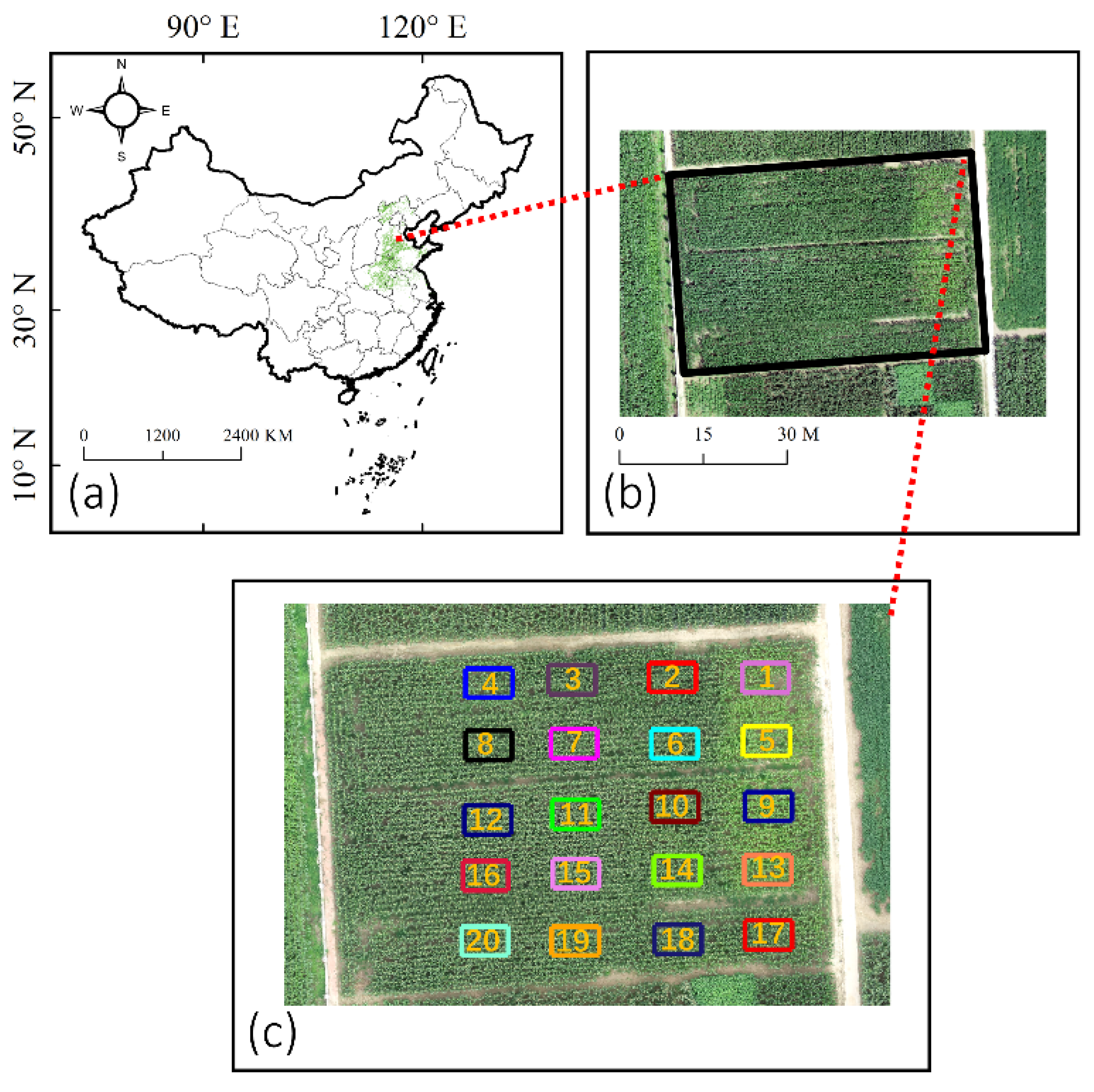
2.1. Study Area

The data collection was conducted in Nanpi Eco-Agricultural Experimental Station (NEES) (38.00°N, 116.40°E) in 2019 (Figure 1). The maize cultivar (Zhengdan 958) was planted on 22 June 2019, and different amounts N, P, and K were applied on 20 plots to optimize the usage of different varieties of fertilizers. One-third of the fertilizers were treated ten days after emergence, another one-third of the fertilizers were treated at booting date, and the remaining fertilizers were treated at heading date (Table A1).
In this study, a DJI Phantom 4 Pro V2.0 was applied for collecting RGB images, and a Mini MCA 6 Camera (MMC) mounted on a DJI M600 Pro UAV platform was conducted to collect multispectral images (Figure 2). The detailed information of the cameras and the deployment of data collection were introduced in previous studies [7,14,26].

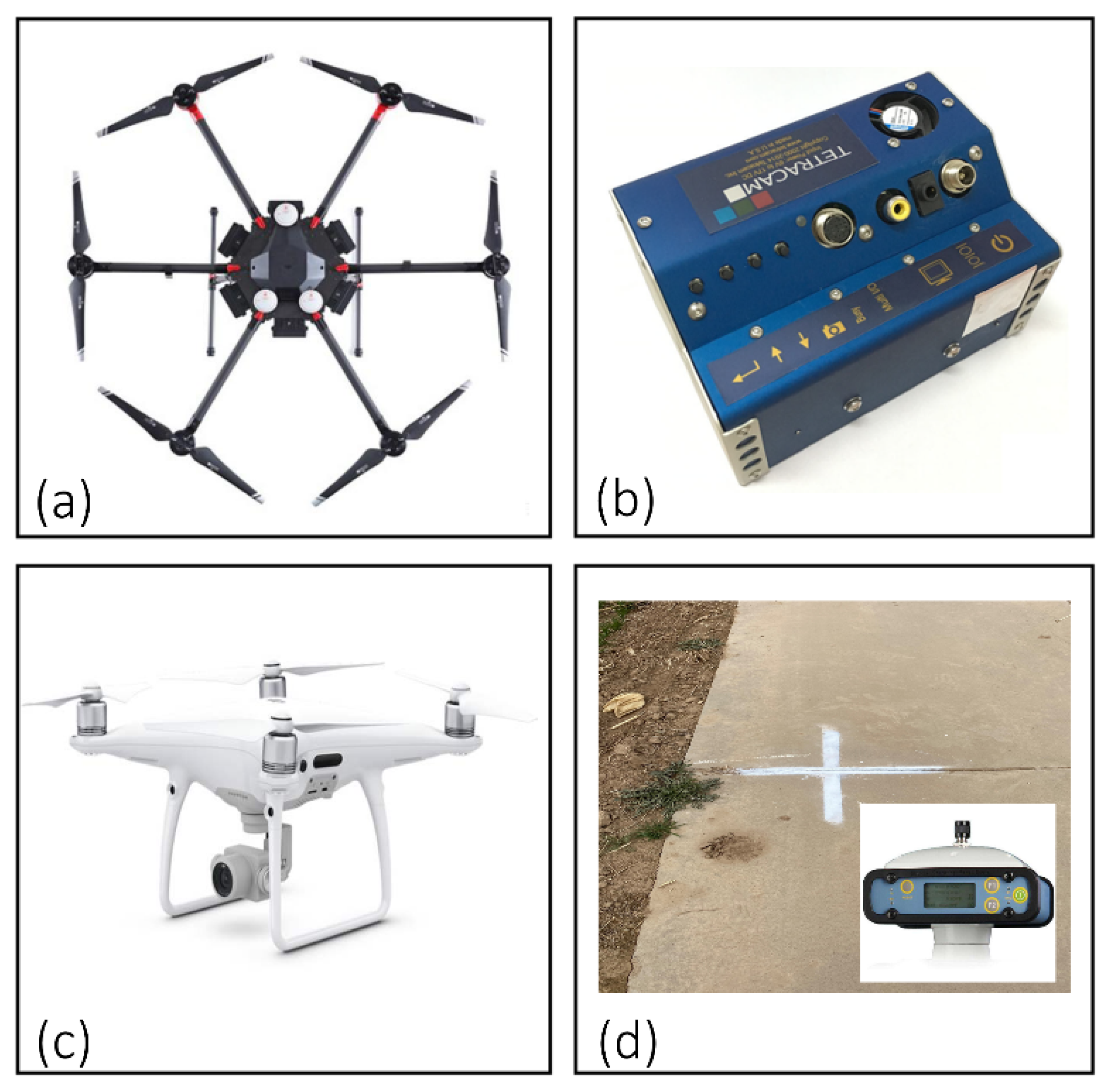
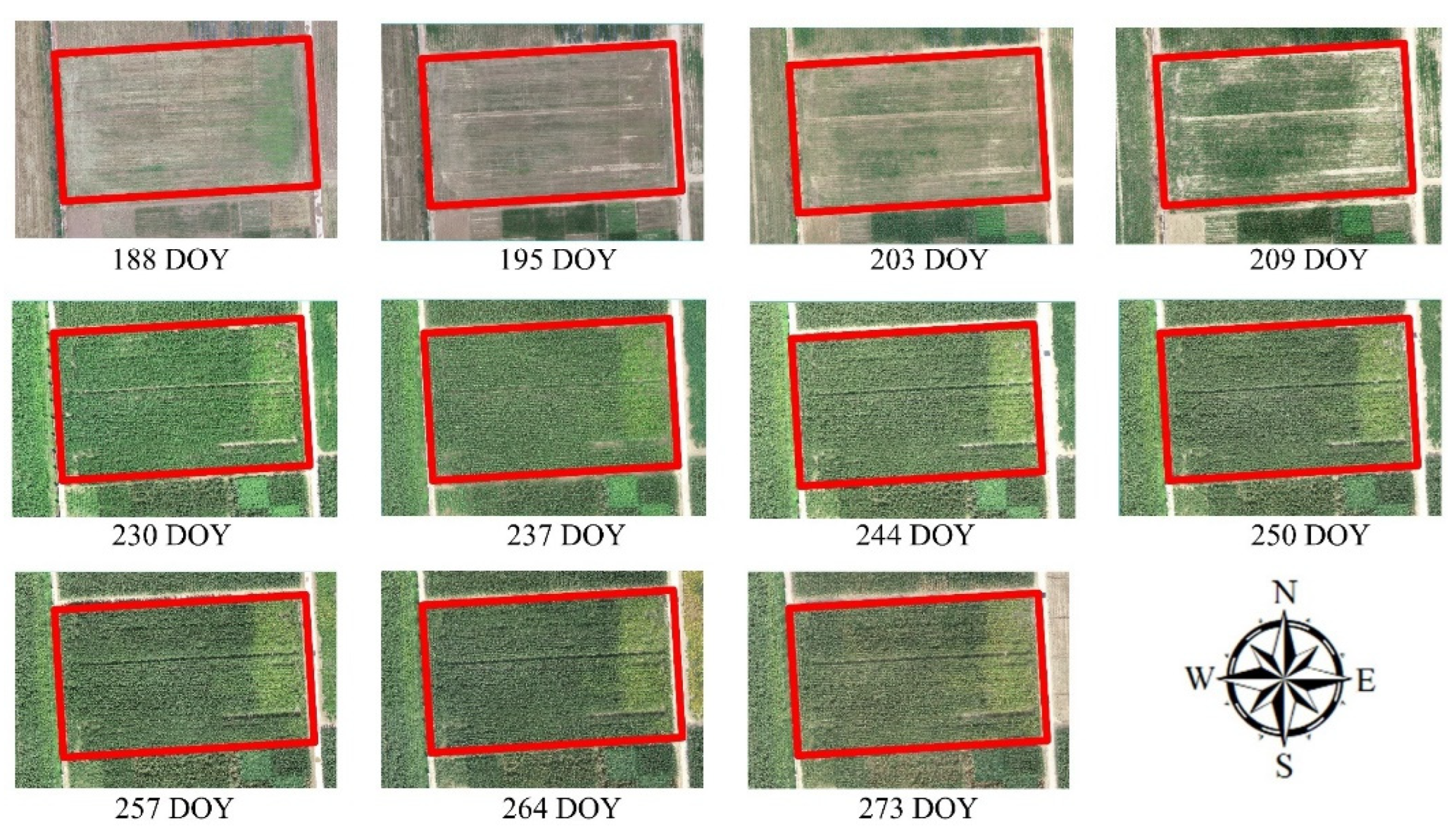
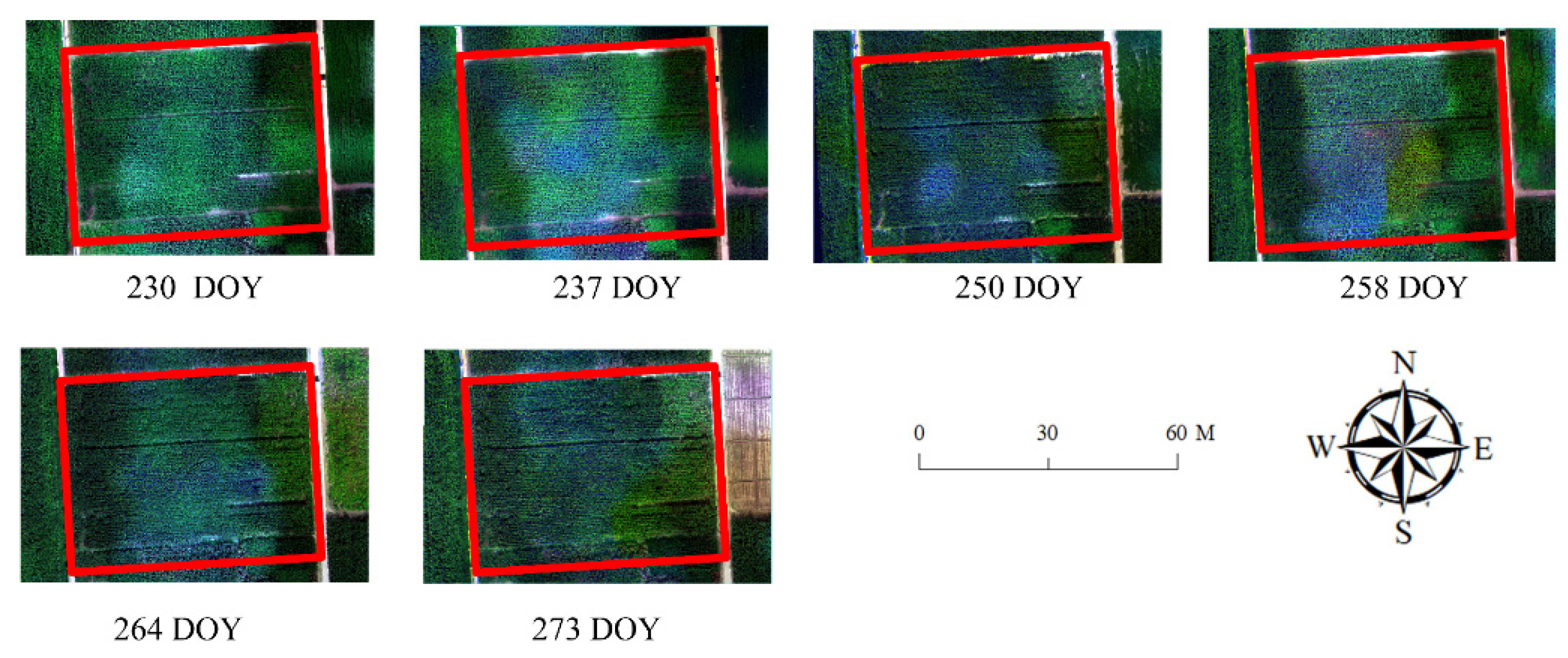
2.2. Data Collection and Preprocessing
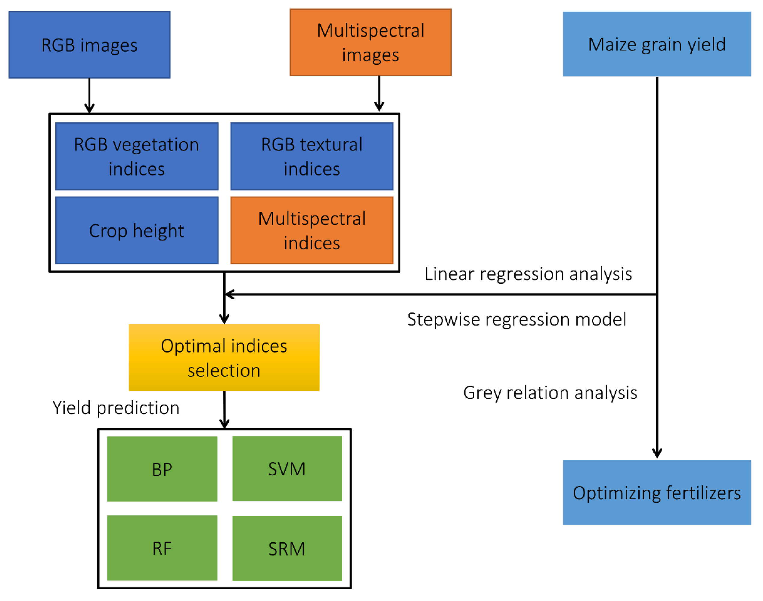
During the entire growth stages of maize, the images were collected on cloudless weather conditions between 11:30 and 12:30 (local time). The maize was seeded on 22 June 2019 and harvested on 5 October 2019; 173 and 278 were the corresponding day of year (DOY), respectively. For the UAV image collection, data collection of the DJI Phantom 4 Pro V2.0 were applied on 188, 195, 203, 209, 230, 237, 244, 250, 257, 264, and 273 DOY and data collection of the MMC were applied on 230, 237, 250, 258, 264, and 273 DOY. To ensure high quality of image acquisition, the forward and side overlaps were set as 85 and 80% for the RGB images acquisition, and 80 and 70% were set for the multispectral image acquisition. Four ground control points (GCPs) were pre-set before the growing season, and the precise locations were obtained using a real-time kinematic (RTK) S86T system (Figure 2d) [23,27]. The single RGB images and multispectral images of each flight were independently mosaicked and processed within Pix4D Mapper under a standard procedure (Lausanne, Switzerland) [28,29]. The images were clipped within IDL (version 8.5) [30]. The spatial resolution of RGB images and multispectral images were 1 and 5 cm, respectively.
Maize grain yields of 20 plots were measured using the format of hundred-grain weight. To reduce the accidental errors of measurement, maize grain yields in each plot were measured three times to avoid accidental errors, and marked as maize grain yield1, maize grain yield2, and maize grain yield3 (Table A1). The final maize grain yield of each plot was obtained as the average of maize grain yield1, maize grain yield2, and maize grain yield3. Through long-time ground observations, it was confirmed that the tasseling dates of most plots happened from 230 to 237 DOY.

2.3. Methods

The workflow was divided into parts: (1) calculating RGB-based VIs, RGB-based TIs, multispectral-based VIs, and maize height; (2) selecting optimal indices and optimal stages for predicitng maize grain yields; (3) predicting maize yield using intergrated optimal indices and machine learning and statictical approaches, i.e., BP, SVM, RF, and stepwise regression model (SRM); (4) optimizating the amounts and varieties of fertilizers using a grey relation analysis. The detailed information is shown in Figure 3.

2.3.1. The Extractions of Spectral Indices/Textural Indices and Maize Height

The RGB images were independently applied to extract the RGB-based VIs, and the first step was to extract the pure pixels only containing maize. Commonly, the D-values between the excess green vegetation index (EXG) and the excess red vegetation index (EXR) have been applied to differentiate maize and soil [31]. The positive D-values were assigned as maize, and the remainder were assigned as soil.
EXG = 2 × G R B
EXR = 1.4 × R G
where R, G, and B denote the original red, green, and blue bands, respectively, of the RGB images. Then, the commonly applied RGB-based VIs were calculated based on RGB images only containing maize (Table 1).
Similarly, commonly applied multispectral-based VIs were extracted (Table 2). The reflectance of soil was quite different from the reflectance of maize in the red band (720 nm) and the near-infrared band (800 nm) [42,43,44]. Then, the pixels that only contained maize and the pixels that only contained soil were sampled, and the reflectance of each was obtained using IDL. It was found that the reflectance lower than 0.04 in the red band and higher than 0.4 in the near-infrared band were defined as maize, and the remaining pixels were defined as soil. Then, various multispectral-based VIs were calculated based on pixels that only contained maize.
The commonly applied TIs such as contrast, correlation, energy, and homogeneity can be extracted from the gray level co-occurrence matrix (GLCM) [61,62], and the red band has been reported to contain slightly more information than the green and blue bands. Therefore, we only applied the red band for extracting the textural information [63]. Since the spatial resolutions of RGB images were higher than multispectral images, the GLCM was calculated using the red bands from RGB images [44,63]. The digital height model (DHM) was obtained using D-values of digital surface model (DSM), to be more specific, the maize height was obtained by subtracting DSM at later growth stages and DSM at earlier stage of growth stage. Thus, the average values of the DHM in each plot were obtained for different growth stages.

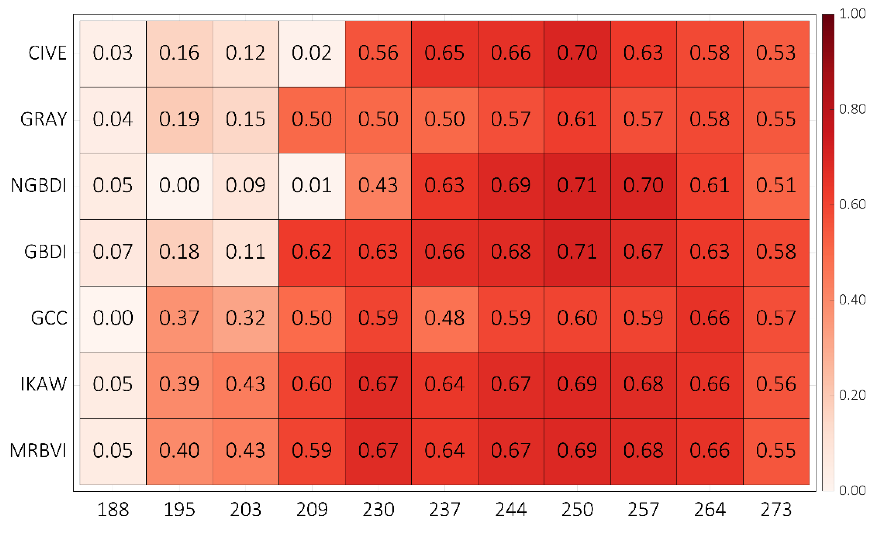
2.3.2. The Selection of Indices and Optimal Growth Stages

The linear regression model (LRM) was separately applied between multi-indicators, namely RGB-based VIs, multispectral-based VIs, RGB-based textural indices, DHM, and maize yields. The indices with higher values of coefficients of determination (R2) were confirmed using the stepwise regression model (SRM). The SRM was applied to select the suitable indices for maize yield prediction with high R2 (p-values significant). Then, the selected indices of all categories were integrated for predicting maize yields. The main purpose of the LRM was to confirm the optimal indices. Evaluating the performance of different indices was not easy, since there was only a limited number of datasets, and to fairly evaluate these indices the selected datasets should be the same for different indices and growth stages. Therefore, we applied all datasets for indice selection, and all sample numbers were used.

2.3.3. The Maize Grain Yield Prediction Using Machine Learning Approaches and Stepwise Regression Model

A backpropagation network (BP) is a typical artificial neural network (ANN) that builds maps between independent and dependent variables iteratively. It has been widely applied to solve problems such as pattern recognition and classification, nonlinear feature extraction, prediction, and function approximation [64]. During the training phase, the BP adjusted the weights while mapping the model output and actual output by minimizing the errors [65,66]. A support vector machine (SVM) that contains linear, polynomial, splines, and radial basis function networks can be applied to handle nearly all problems of regression [67]. Random forest (RF) can automatically measure the contribution of independent variables and adjust the tree structure of the model. A RF classifier can build massive and multi-layers of trees for simulating (regression and classification), and it can also test the relatively importance of independent variable.
In this study, the selected indices were integrated for predicting maize grain yields using advanced machine learning methods and the traditional stepwise regression model (SRM) method. To be more specific, the optimal indices were treated as the independent variables and the corresponding maize grain yields of each plot were treated as the dependent variables. In order to fully use the dataset, a 10-fold cross-validation was applied. The whole dataset was divided into 10 parts, i.e., 9 parts for training the model and 1 part for model validating. For the BP, the parameters were set as: maximum training times, 10,000; minimum error of training target, 1e-6; learning rate, 0.001; and maximum number of confirmation failures, 1000. For the RF, the number of trees was set as default 500, the bootstrap was set as true, and the number of variables used for the binary tree in the node was set as max of floor (D/3). For the SVM, the kernel-type was set as linear, u’*v; c cost and g gamma were optimized using the grid search method (x and y each ranged from −5 to 5 with an interval of 0.1); the SVM type was set as epsilon-SVR; and the p epsilon was set as 0.01 [68,69]. For the SRM, the multiple linear regression method was applied.
The commonly applied indicators R2 and root mean square error (RMSE) were adopted to evaluate model performance [23]. The built-in model with the lowest RMSE and highest R2 was retained for further maize grain yield mapping. For different sources of data, the RGB images were resized to the same resolution of the multispectral images. The coefficients in the well-built models were each applied to predict the maize grain yield using the selected indices at optimal growth stages.

2.3.4. The Confirmation of Optimal Amounts and Combinations of Fertilizers

The different amounts and combinations of N, P, and K and maize grain yields were applied for further analysis to confirm the optimal amounts and combinations of fertilizers. A grey relation analysis (GRA) is commonly conducted in agriculture for assessing the relationships of correlated variables [70,71]. In particular, a GRA is an excellent method for calculating the grey relational degree and determining the contribution measure of the main behavior of a system or the influence degree between system factors. A GRA was applied to assess the relative importance of fertilizers to maize grain yields. The independent variables were the amounts of fertilizers of 20 plots in sequences, and the dependent variables were the corresponding maize grain yields in sequences. The values of the GRCsfor the fertilizer were compared, and the most important fertilizers were obtained. The ratios of fertilizers were applied and the suggested usages of fertilizers were confirmed.

3. Results

3.1. The Linear Regression Analysis between Indices and Maize Grain Yields

The RGB images and multispectral images acquired at different growth stages of maize were processed under a standard procedure using the approach introduced in the Methods section (Figure A1 and Figure A2). To better show the difference between different growth stages, the images were all shown in the RGB color system for comparison. The tasseling dates of maize in all plots mostly happened from 230 to 237 DOY.
The RGB-based VIs of 20 plots during the entire growth stages of maize were linear regressed with maize grain yields. The RGB-based VI with regression equations, R2 and p-values are shown in Table 3. It can be obtained that R2 ranged from 0.748 to 0.809, indicating that RGB-based VIs were closely correlated with maize grain yields. It can be deduced that the RGB-based VIs may have great potential for predicting maize grain yields.
The multispectral-based VIs during the entire growth stages was also linear regressed with maize grain yields. The multispectral-based VIs with regression equations, R2, and p-values are shown in Table 4. It can be obtained that the R2 of multispectral-based VIs ranged from 0.780 to 0.826, and these values were slightly higher than those of RGB-based VIs.
The TIs including contrast, correlation, energy, homogeneity and the DHM were independently extracted from the RGB images, and a linear regression analysis was conducted between these indices and maize grain yields. The linear regression results using textural indices and DHM are shown in Table 5. It can be observed that the R2 values ranged from 0.779 to 0.901, and the R2 values were larger than the values of the multispectral-based VIs, except for energy. Thus, the textural indices were closely correlated with maize grain yields. The DHM also had a close relationship with the yield, of which the R2 was 0.857.

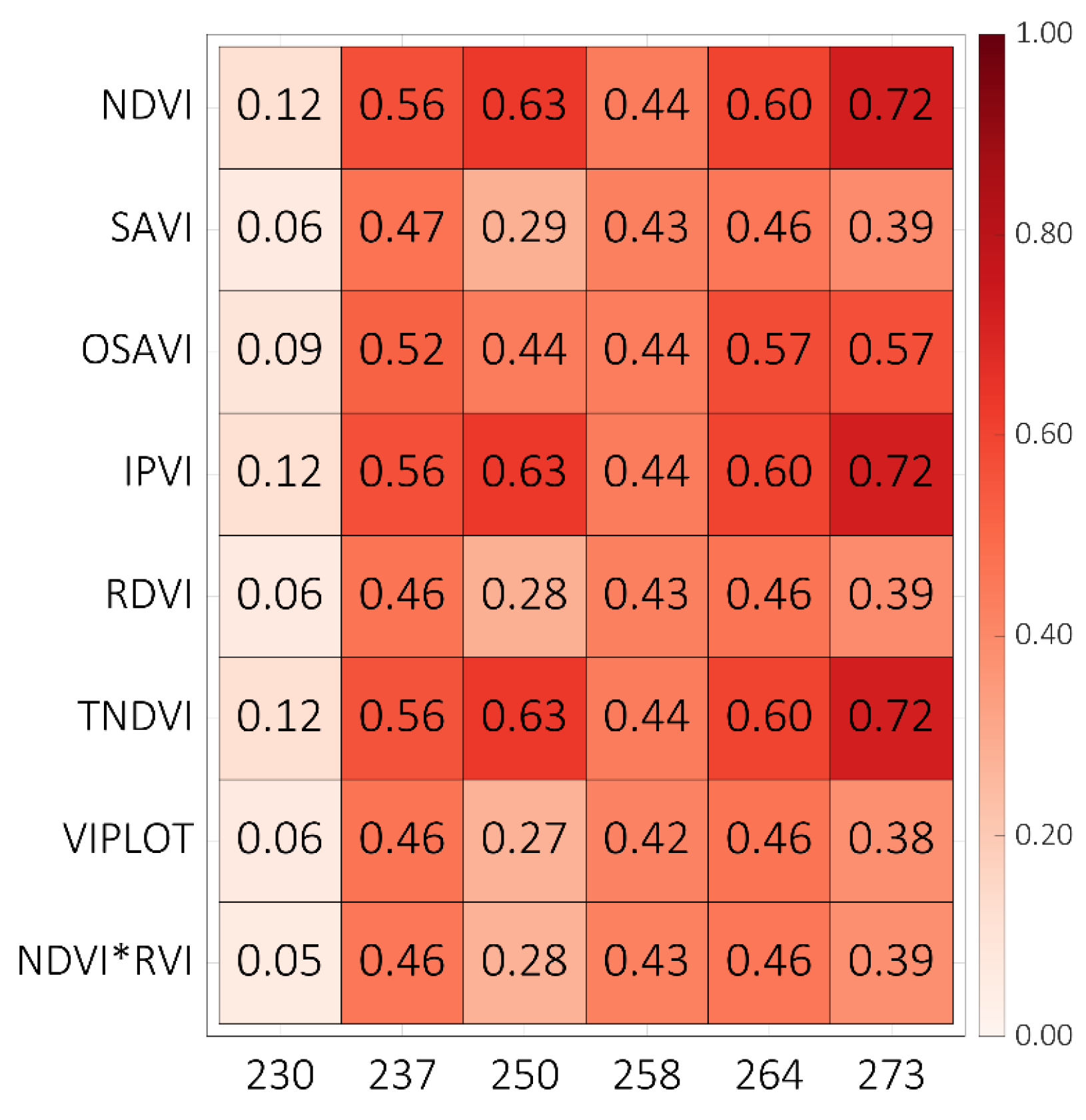
3.2. The Selection of Optimal Growth Stage for Maize Grain Yield Prediction

The RGB-based VIs of 20 plots at each growth period were linearly regressed with maize grain yields (Figure 4). It can be observed that the R2 using data collected from 230 to 273 DOY were commonly larger than those during the period from 188 to 209 DOY. The data acquired on 250 DOY achieved the highest R2, of which the value was 0.71 for NGBDI and GBDI. The data collected from 230 to 273 DOY were more correlated with maize grain yields than the data collected from 188 to 209 DOY. The RGB-based VIs from 230 to 273 DOY were selected for maize grain yield prediction.
The multispectral-based VIs of 20 plots at different growth periods were separately linear regressed with maize grain yields (Figure 5). The data collected on 237 DOY were more correlated with maize grain yields. The tasseling dates ranged from 230 to 237 DOY for 20 plots, and the higher R2 values achieved from 230 DOY indicated that the accuracy of yield prediction using data collected from tasseling date to maturity date was higher. The multispectral-based VIs from 230 to 273 DOY were selected for further predicting maize grain yields.

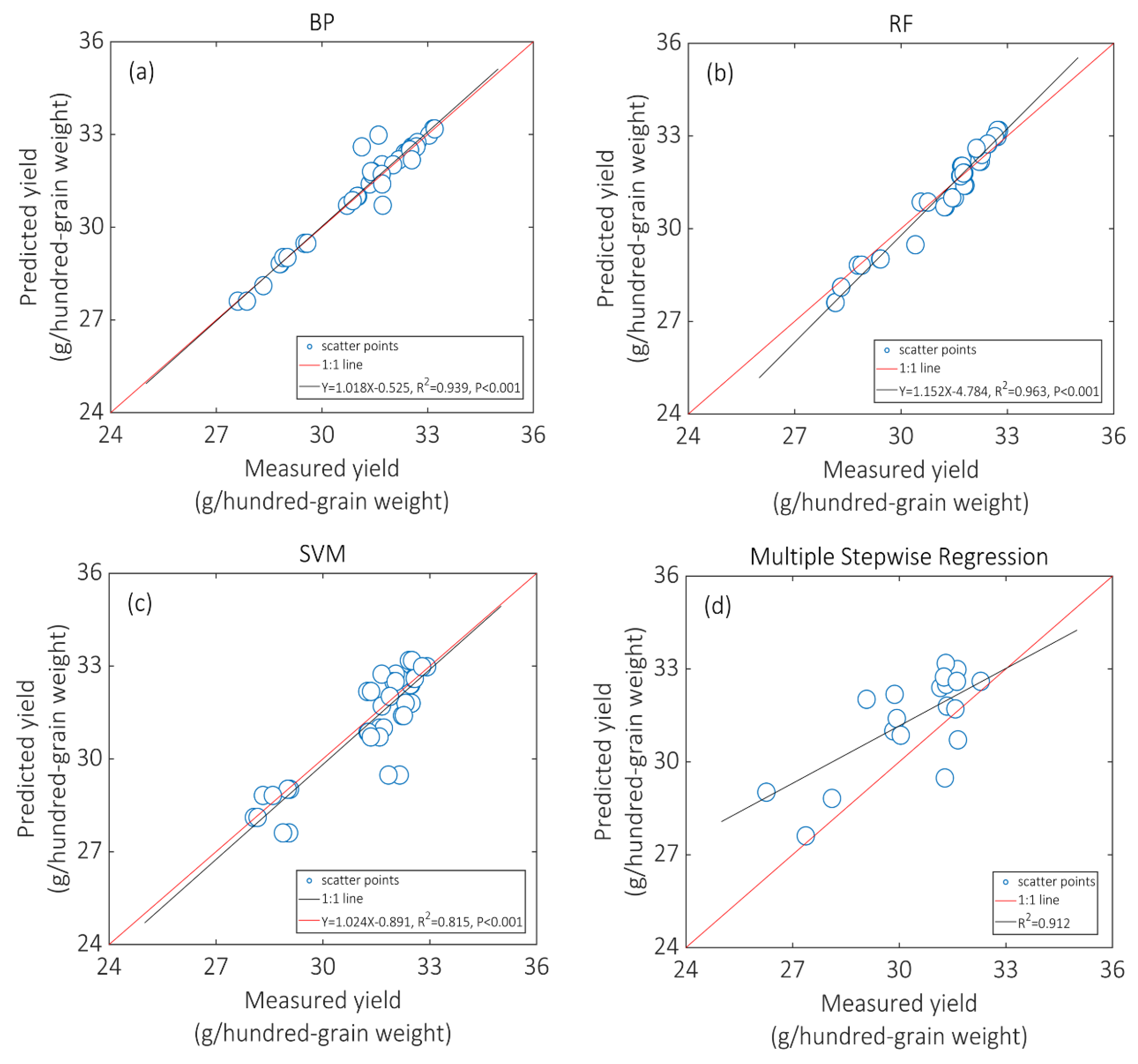
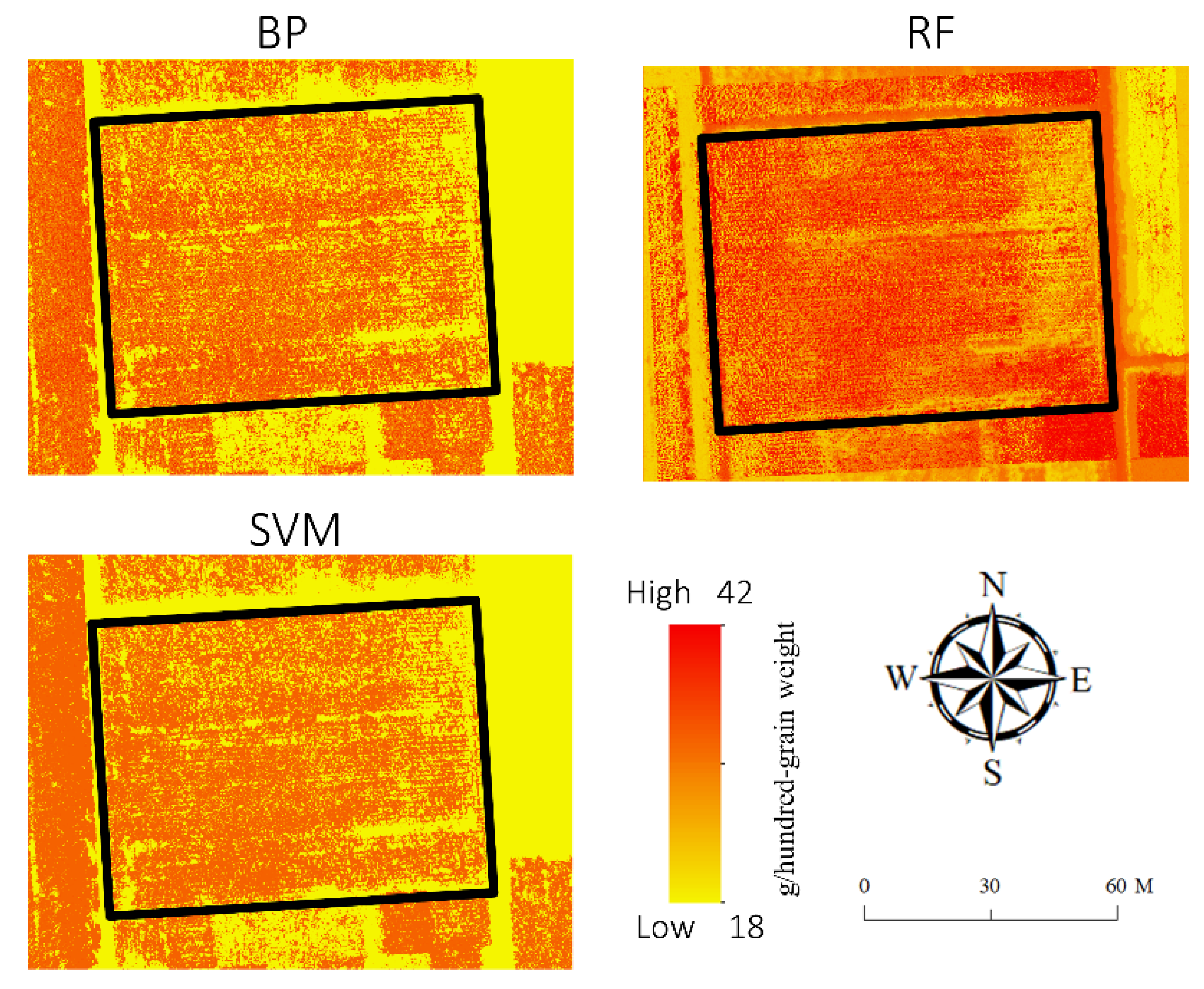
3.3. The Maize Grain Yield Prediction of Maize Using Machine Learning Methods and Traditional Regression Method

The selected RGB-based VIs, multispectral-based VIs, RGB-based textural indices, and DHM at optimal growth stages were integrated to predict maize grain yields using three machine learning methods, i.e., BP, SVM, RF, and a traditional regression method, i.e., SRM. Each model was independently applied to build the relationships between these integrated indices and maize grain yields. The comparison of measured and predicted maize grain yields are shown in Figure 6.
For the machine learning-based methods, the R2 values using BP, RF, and SVM were 0.939, 0.963, and 0.815, respectively. Similarly, the RMSE values using BP, RF, and SVM were 0.496, 0.489, and 0.823 g/hundred-grain weight, respectively. The BP and RF both performed better than SVM, with higher R2 values and lower RMSE values. For the results using SRM, the R2 was 0.912, and the RMSE was 1.772 g/hundred-grain weight. Therefore, the machine learning-based methods have greater potential for predicting maize grain yield, and the RF achieved the highest accuracy. The optimized parameters of the machine learning-based models were applied for mapping maize grain yields (pixel-based optimal indices collected at optimal growth stages) (Figure 7).

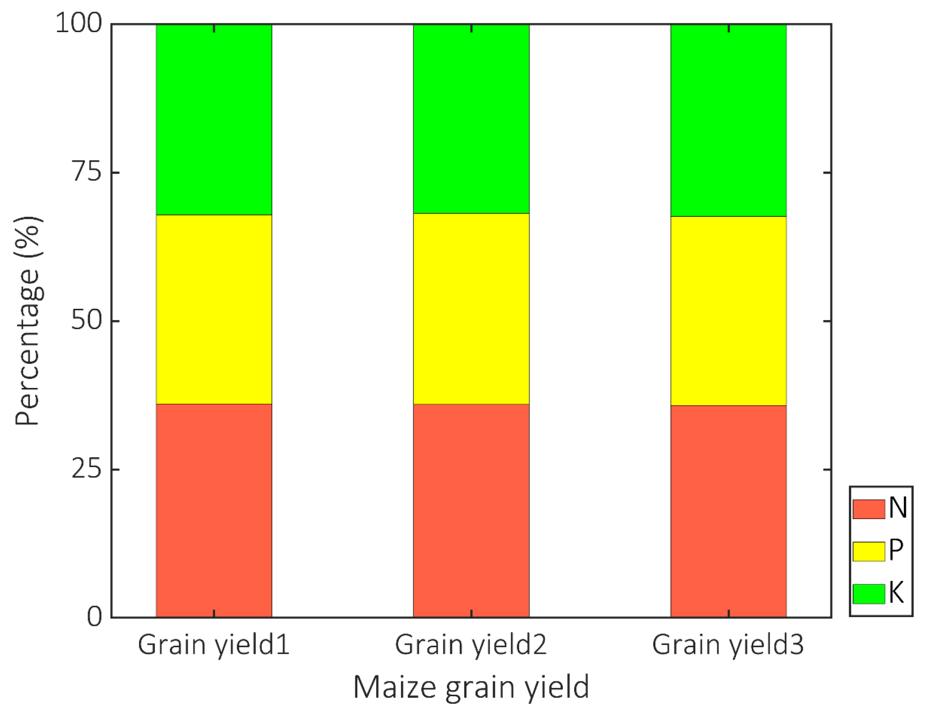
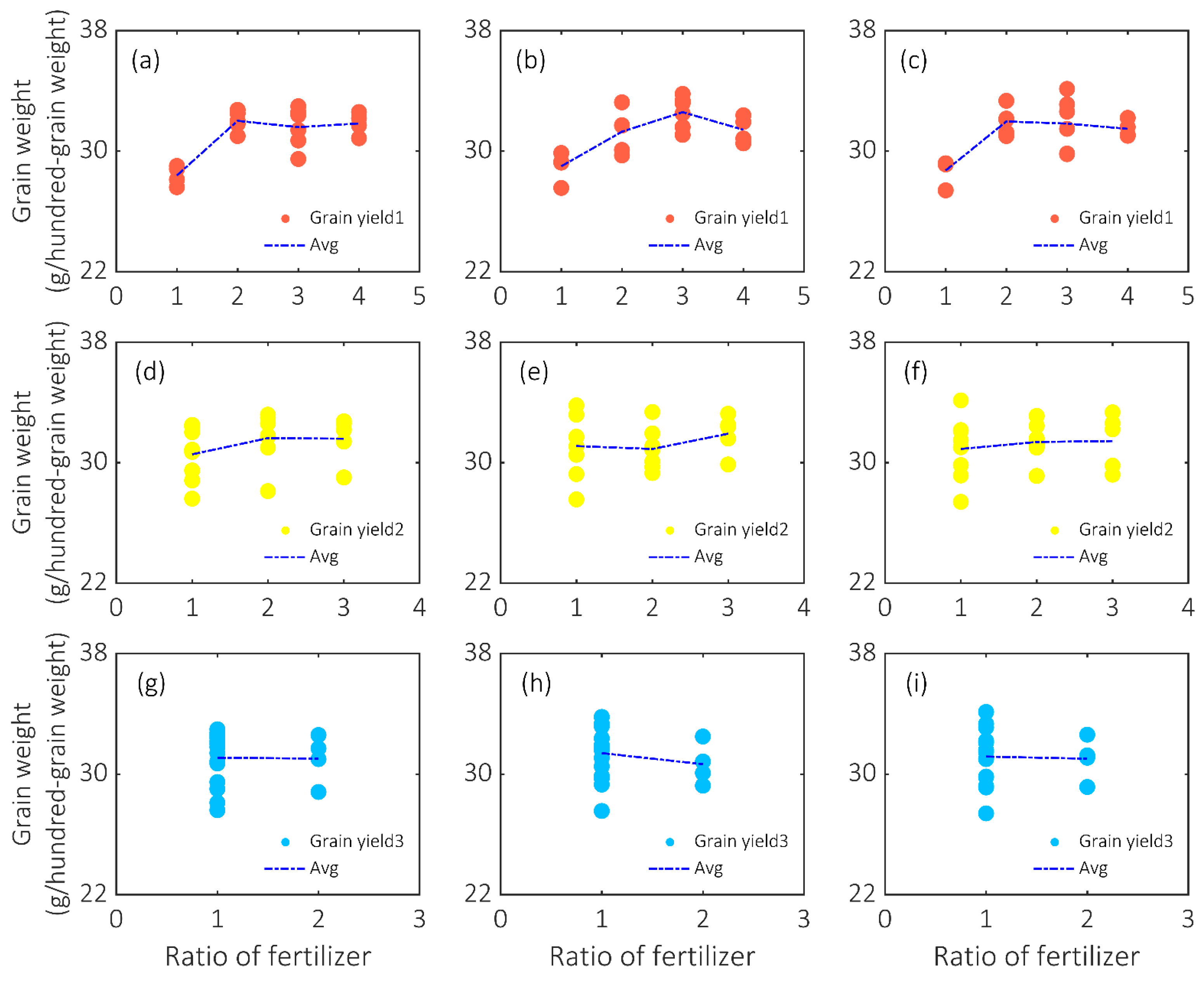
3.4. The Optimization of Combinations and Rations for Fertilizers

The grey relation coefficients (GRCs) between each type of fertilizer and yields calculated using the grey relation analysis (GRA) are shown in Figure 8. The GRC values were 35.707, 34.435, and 29.857% for the maize grain yield1, 36.417, 32.606, 30.975% for maize grain yield2, and 35.926, 33.084, and 30.989% for maize grain yield3. The results show that N is the dominating influencing factor for the growth of maize.
The changes in N, K, and P fertilizers with the corresponding variations of maize grain yields are shown in Figure 9. It can be clearly noted that the impacts of different ratios of fertilizer to maize grain yields varied significantly. For N, the maize grain yields increased with the addition of N, until the ratios increased between 2 and 3 (Figure 9a–c). The optimal application ratio of N was 2. For P and K, the maize grain yields merely changed with the adding of these two fertilizers. Most of the circumstances in subplots from Figure 9d to Figure 9i showed decreased maize grain yields due to the increased usage of P and K. The optimal application ratios for P and K was 1. It can be deduced that the optimal combination ratio of N/P/K is 2:1:1.

4. Discussion

4.1. Yield Prediction Using Multi-Source Data from a UAV Platform

In this study, the RGB images and multispectral images covering the entire growth stages of maize were collected from a UAV platform. The selected RGB-based VIs, TIs, and DHM from RGB images, and the multispectral-based VIs were integrated for predicting maize grain yields. The R2 values of yield prediction only using RGB-based VIs ranged from 0.748 to 0.809 during the growing season. The RGB-based VIs were closely correlated with maize grain yields. The results were consistent with previous studies, where RGB-based VIs from RGB images were proven to have great potential for agricultural yield predictions [7]. The multispectral-based VIs performed slightly better than the RGB-based VIs. This was also consistent with previous studies, where multispectral-based VIs were found to have greater potential than RGB-based VIs in predicting agricultural yields [72,73,74]. Unlike the satellite-based images, the UAV-based RGB and multispectral images were commonly at the centimeter level, and were merely influenced by the mixed pixels. The high-resolution images from a UAV can be applied to derive high-resolution textural indices. We found the TIs with the DHM also improved the accuracy of maize grain yield prediction, with R2 values ranging from 0.779 to 0.901. The TIs actually expressed the dynamic changes of maize in a different way from spectral indices [75,76,77]. The DHM was actually the crop phenotype, and it was found to be very useful for predicting crop yields [78,79,80].
The R2 values between maize grain yields and indices were totally different for different growth stages. The higher R2 values occurred from 230 to 237 DOY; this stage (tasseling date) was in accordance with previous studies, and was found to be closely correlated with maize grain yields [81,82,83]. Therefore, tasseling date is an important phenology for yield prediction, and the data collected during this period are important for assessing maize grain yields. Meanwhile, tasseling date has been widely proven to be an important period for management practices such as the application of fertilizers [84,85,86,87]. Therefore, it was recommended to integrate RGB-based VIs, RGB-based TIs, multispectral-based VIs, and DHM (maize height) acquired from tasseling date to maturity date for predicting maize grain yields.
N was found to be the most important fertilizer to increase maize grain yields. This founding was in accordance with previous studies where the application of N was correlated with maize grain yields [88,89,90]. Increasing the ratios of P and K was also greatly correlated with maize grain yields. Therefore, it was suggested that the optimal ratio of N/P/K was 2:1:1. Excessive application of fertilizers to agricultural land can cause uneven distribution of resources, and can reduce the potential application of fertilizers to other fields where materials are needed [91,92,93,94]. In addition, excessive application of fertilizers can cause serious land degradation, endangering the environmental and ecological system, and lead to a reduction in agricultural yields. There is a need to reduce the potential usage of P and K, since the added P and K will reduce agricultural yields and also destroy valuable cultivated land. This is very important to meet the requirement of sustainable agriculture.

4.2. The Limitations

Multi-sources of UAV images were applied for predicting maize grain yields using traditional regression and advanced machine learning approaches. The data quality was strictly controlled, but there were uncertainties that still remained from the data source and data processing. First, there was a mismatch between the geometric registration between the RGB images (1 cm) and multispectral images (5 cm), even though the RGB images were resampled to the same spatial resolution as the multispectral images. This would influence the extraction of various VIs, and would further influence the maize grain yield predictions. Second, the images covering the entire growth of maize were collected under similar imaging conditions, but there were slight differences in the solar radiation, wind, air pressure, and atmospheric effects. These differences in environmental conditions would influence the image collection. In addition, the long working time of cameras and the hot temperature would create inevitable noise, especially in summer [95,96]. Third, the applied machine learning methods were commonly used methods; more advanced machine learning and deep learning methods that would certainly achieve high accuracy in yield predictions could be explored in future analysis [97,98,99]. Finally, the number of sampling plots was limited in this study, which may cause an overfitting problem. A larger number of plots for exploring different amounts and combinations of fertilizers on maize grain yield could be conducted in future analysis. Machine learning-based approaches using more datasets may realize more reasonable and convincing results.

5. Conclusions

In this study, the multi-indicators, namely RGB-based VIs, RGB-based TIs, multispectral-based VIs, and maize height from UAV data were applied for predicting maize grain yields. The RGB-based VIs and multispectral-based VIs were proven to be closely correlated with maize grain yields. The innovation of integration of commonly applied VIs, Tis, and crop height for maize grain yield prediction significantly improved the accuracy. The data collected from tasseling date to maturity date were more correlated with the maize grain yield than other phenological growth stages. The tasseling date is an important phenology of maize that would promote the accuracy of yield prediction of summer maize. The multi-indicators were integrated to predict maize grain yields using traditional regression and advanced machine learning approaches. The machine learning approaches were commonly better than the traditional regression method, and R gained the highest accuracy (R2 = 0.963 and RMSE = 0.489 g/hundred-grain weight). It is recommended to adopt multi-data (spectral, textural indices, and maize height) from tasseling date to maturity date for predicting maize grain yields based on RF.

Author Contributions

Conceptualization, Y.G. and X.Z.; methodology, Y.G. and X.Z.; software, Y.G. and S.C.; validation, Y.G., X.Z., S.C. and H.W.; formal analysis, H.W. and S.J.; investigation, S.J. and D.C.; resources, Y.G., X.Z. and Y.F.; data curation, Y.G., X.Z., D.C. and Y.F.; writing—original draft preparation, Y.G.; writing—review and editing, Y.G., X.Z. and Y.F.; visualization, Y.G.; supervision, X.Z. and Y.F.; project administration, X.Z.; funding acquisition, X.Z. and Y.F. All authors have read and agreed to the published version of the manuscript.

Funding

This study was funded by the National Natural Science Foundation of China (Grant No. 41907157), the joint fund for regional innovation and development of NSFC (Grant No. U21A2039), the National Funds for Distinguished Young Youths (Grant No. 42025101), and the 111 Project (Grant No. B18006).

Data Availability Statement

Data will be made available on request.

Acknowledgments

We thank deeply all workers from Nanpi Eco-Agricultural Experimental Station (NEES) for their support of the data collection. We thank Hongyong Sun from NEES for providing the convenience for data collection.

Conflicts of Interest

The authors declare no conflict of interest.

Appendix A

Figure A1. The RGB images at different growth stages of maize.
Remotesensing 14 06290 g0a1
Figure A2. The multispectral images at different growth stages of maize.
Remotesensing 14 06290 g0a2
Table A1. The application of fertilizers in 20 plots. The number after NPK represents the actual multiple applications of fertilizers. The plots correspond to the plots shown in Figure 1. The 1, 2, and 3 each represent 0.7, 1.4, and 2.1 kg of the elements, respectively.
PlotsCombinationsGrain Yield 1Grain Yield 2Grain Yield 3
1N1P1K228.8229.2429.15
2N3P1K129.4831.0829.84
3N3P3K131.431.629.8
4N2 + wheat-straw32.0231.732.1
5N1P1K127.6127.5627.4
6N3P3K232.632.532.62
7N3P2K132.9833.3633.1
8N2 + Organic material33.1831.132.44
9N1P2K128.1129.3129.12
10N2P2K23130.0831.25
11N4P3K132.1832.3832.21
12N3+ wheat-straw30.7133.831.48
13N1P3K129.0229.8829.2
14N2P1K132.531.7232.16
15N4P2K132.631.9431.6
16N3 + Organic material32.433.1834.13
17N2P3K132.7433.2433.34
18N2P2K131.829.7231
19N4P1K130.8630.5231.02
20N4P2K231.7130.8431.09

References

  1. Zhao, C.; Liu, B.; Piao, S.; Wang, X.; Lobell, D.B.; Huang, Y.; Huang, M.; Yao, Y.; Bassu, S.; Ciais, P. Temperature increase reduces global yields of major crops in four independent estimates. Proc. Natl. Acad. Sci. USA 2017, 114, 9326–9331. [Google Scholar] [CrossRef] [PubMed] [Green Version]
  2. Asseng, S.; Ewert, F.; Martre, P.; Rötter, R.P.; Lobell, D.B.; Cammarano, D.; Kimball, B.A.; Ottman, M.J.; Wall, G.; White, J.W. Rising temperatures reduce global wheat production. Nat. Clim. Chang. 2015, 5, 143–147. [Google Scholar] [CrossRef]
  3. Van Vuuren, D.P.; Stehfest, E.; den Elzen, M.G.; Kram, T.; van Vliet, J.; Deetman, S.; Isaac, M.; Goldewijk, K.K.; Hof, A.; Beltran, A.M. RCP2. 6: Exploring the possibility to keep global mean temperature increase below 2 C. Clim. Chang. 2011, 109, 95–116. [Google Scholar] [CrossRef]
  4. Zhu, W.; Sun, Z.; Peng, J.; Huang, Y.; Li, J.; Zhang, J.; Yang, B.; Liao, X. Estimating maize above-ground biomass using 3D point clouds of multi-source unmanned aerial vehicle data at multi-spatial scales. Remote Sens. 2019, 11, 2678. [Google Scholar] [CrossRef] [Green Version]
  5. Bockman, O.C.; Kaarstad, O.; Lie, O.H.; Richards, I. Agriculture and Fertilizers; Scientific Publishers: Jodhpur, India, 2015. [Google Scholar]
  6. Horrigan, L.; Lawrence, R.S.; Walker, P. How sustainable agriculture can address the environmental and human health harms of industrial agriculture. Environ. Health Perspect. 2002, 110, 445–456. [Google Scholar] [CrossRef] [Green Version]
  7. Guo, Y.; Wang, H.; Wu, Z.; Wang, S.; Sun, H.; Senthilnath, J.; Wang, J.; Robin Bryant, C.; Fu, Y. Modified red blue vegetation index for chlorophyll estimation and yield prediction of maize from visible images captured by UAV. Sensors 2020, 20, 5055. [Google Scholar] [CrossRef]
  8. Weiss, M.; Jacob, F.; Duveiller, G. Remote sensing for agricultural applications: A meta-review. Remote Sens. Environ. 2020, 236, 111402. [Google Scholar] [CrossRef]
  9. Cammarano, D.; Basso, B.; Holland, J.; Gianinetti, A.; Baronchelli, M.; Ronga, D. Modeling spatial and temporal optimal N fertilizer rates to reduce nitrate leaching while improving grain yield and quality in malting barley. Comput. Electron. Agric. 2021, 182, 105997. [Google Scholar] [CrossRef]
  10. Lobell, D.B.; Burke, M.B. On the use of statistical models to predict crop yield responses to climate change. Agric. For. Meteorol. 2010, 150, 1443–1452. [Google Scholar] [CrossRef]
  11. Bhardwaj, A.; Sam, L.; Martín-Torres, F.J.; Kumar, R. UAVs as remote sensing platform in glaciology: Present applications and future prospects. Remote Sens. Environ. 2016, 175, 196–204. [Google Scholar] [CrossRef]
  12. Matese, A.; Toscano, P.; Di Gennaro, S.F.; Genesio, L.; Vaccari, F.P.; Primicerio, J.; Belli, C.; Zaldei, A.; Bianconi, R.; Gioli, B. Intercomparison of UAV, aircraft and satellite remote sensing platforms for precision viticulture. Remote Sens. 2015, 7, 2971–2990. [Google Scholar] [CrossRef] [Green Version]
  13. Zeng, L.; Wardlow, B.D.; Xiang, D.; Hu, S.; Li, D. A review of vegetation phenological metrics extraction using time-series, multispectral satellite data. Remote Sens. Environ. 2020, 237, 111511. [Google Scholar] [CrossRef]
  14. Guo, Y.; Yin, G.; Sun, H.; Wang, H.; Chen, S.; Senthilnath, J.; Wang, J.; Fu, Y. Scaling effects on chlorophyll content estimations with RGB camera mounted on a UAV platform using machine-learning methods. Sensors 2020, 20, 5130. [Google Scholar] [CrossRef] [PubMed]
  15. Wan, L.; Cen, H.; Zhu, J.; Zhang, J.; Zhu, Y.; Sun, D.; Du, X.; Zhai, L.; Weng, H.; Li, Y. Grain yield prediction of rice using multi-temporal UAV-based RGB and multispectral images and model transfer–a case study of small farmlands in the South of China. Agric. For. Meteorol. 2020, 291, 108096. [Google Scholar] [CrossRef]
  16. Senthilnath, J.; Dokania, A.; Kandukuri, M.; Ramesh, K.; Anand, G.; Omkar, S. Detection of tomatoes using spectral-spatial methods in remotely sensed RGB images captured by UAV. Biosyst. Eng. 2016, 146, 16–32. [Google Scholar] [CrossRef]
  17. Liu, Y.; Feng, H.; Yue, J.; Fan, Y.; Jin, X.; Zhao, Y.; Song, X.; Long, H.; Yang, G. Estimation of Potato Above-Ground Biomass Using UAV-Based Hyperspectral images and Machine-Learning Regression. Remote Sens. 2022, 14, 5449. [Google Scholar] [CrossRef]
  18. Wang, F.; Yi, Q.; Hu, J.; Xie, L.; Yao, X.; Xu, T.; Zheng, J. Combining spectral and textural information in UAV hyperspectral images to estimate rice grain yield. Int. J. Appl. Earth Obs. Geoinf. 2021, 102, 102397. [Google Scholar] [CrossRef]
  19. Zha, H.; Miao, Y.; Wang, T.; Li, Y.; Zhang, J.; Sun, W.; Feng, Z.; Kusnierek, K. Improving Unmanned Aerial Vehicle Remote Sensing-Based Rice Nitrogen Nutrition Index Prediction with Machine Learning. Remote Sens. 2020, 12, 215. [Google Scholar] [CrossRef] [Green Version]
  20. Wan, L.; Zhang, J.; Dong, X.; Du, X.; Zhu, J.; Sun, D.; Liu, Y.; He, Y.; Cen, H. Unmanned aerial vehicle-based field phenotyping of crop biomass using growth traits retrieved from PROSAIL model. Comput. Electron. Agric. 2021, 187, 106304. [Google Scholar] [CrossRef]
  21. Amelong, A.; Gambín, B.; Severini, A.D.; Borrás, L. Predicting maize kernel number using QTL information. Field Crops Res. 2015, 172, 119–131. [Google Scholar] [CrossRef]
  22. Senthilnath, J.; Kandukuri, M.; Dokania, A.; Ramesh, K. Application of UAV imaging platform for vegetation analysis based on spectral-spatial methods. Comput. Electron. Agric. 2017, 140, 8–24. [Google Scholar] [CrossRef]
  23. Guo, Y.; Chen, S.; Li, X.; Cunha, M.; Jayavelu, S.; Cammarano, D.; Fu, Y. Machine Learning-Based Approaches for Predicting SPAD Values of Maize Using Multi-Spectral Images. Remote Sens. 2022, 14, 1337. [Google Scholar] [CrossRef]
  24. Shu, M.; Fei, S.; Zhang, B.; Yang, X.; Guo, Y.; Li, B.; Ma, Y. Application of UAV Multisensor Data and Ensemble Approach for High-Throughput Estimation of Maize Phenotyping Traits. Plant Phenomics 2022, 2022, 1–17. [Google Scholar] [CrossRef]
  25. Li, L.; Wang, B.; Feng, P.; Li Liu, D.; He, Q.; Zhang, Y.; Wang, Y.; Li, S.; Lu, X.; Yue, C. Developing machine learning models with multi-source environmental data to predict wheat yield in China. Comput. Electron. Agric. 2022, 194, 106790. [Google Scholar] [CrossRef]
  26. Guo, Y.; Senthilnath, J.; Wu, W.; Zhang, X.; Zeng, Z.; Huang, H. Radiometric calibration for multispectral camera of different imaging conditions mounted on a UAV platform. Sustainability 2019, 11, 978. [Google Scholar] [CrossRef] [Green Version]
  27. Qiao, Q.; Li, C.; Jing, H.; Huang, L. Flow structure and channel morphology after artificial chute cutoff at the meandering river in the upper Yellow River. Arab. J. Geosci. 2022, 15, 1–19. [Google Scholar] [CrossRef]
  28. Barrero, O.; Perdomo, S.A. RGB and multispectral UAV image fusion for Gramineae weed detection in rice fields. Precis. Agric. 2018, 19, 809–822. [Google Scholar] [CrossRef]
  29. Taddia, Y.; Russo, P.; Lovo, S.; Pellegrinelli, A. Multispectral UAV monitoring of submerged seaweed in shallow water. Appl. Geomat. 2020, 12, 19–34. [Google Scholar] [CrossRef] [Green Version]
  30. Shaharum, N.S.N.; Shafri, H.Z.M.; Gambo, J.; Abidin, F.A.Z. Mapping of Krau Wildlife Reserve (KWR) protected area using Landsat 8 and supervised classification algorithms. Remote Sens. Appl. Soc. Environ. 2018, 10, 24–35. [Google Scholar] [CrossRef]
  31. Meyer, G.E.; Neto, J.C. Verification of color vegetation indices for automated crop imaging applications. Comput. Electron. Agric. 2008, 63, 282–293. [Google Scholar] [CrossRef]
  32. Kajita, S.; Kanehiro, F.; Kaneko, K.; Fujiwara, K.; Harada, K.; Yokoi, K.; Hirukawa, H. Biped walking pattern generation by using preview control of zero-moment point. In Proceedings of the 2003 IEEE International Conference on Robotics and Automation (Cat. No. 03CH37422), Taipei, Taiwan, 14–19 September 2003; pp. 1620–1626. [Google Scholar]
  33. Saberioon, M.; Amin, M.; Anuar, A.; Gholizadeh, A.; Wayayok, A.; Khairunniza-Bejo, S. Assessment of rice leaf chlorophyll content using visible bands at different growth stages at both the leaf and canopy scale. Int. J. Appl. Earth Obs. Geoinf. 2014, 32, 35–45. [Google Scholar] [CrossRef]
  34. Louhaichi, M.; Borman, M.M.; Johnson, D.E. Spatially located platform and aerial photography for documentation of grazing impacts on wheat. Geocarto Int. 2001, 16, 65–70. [Google Scholar] [CrossRef]
  35. Kazmi, W.; Garcia-Ruiz, F.J.; Nielsen, J.; Rasmussen, J.; Andersen, H.J. Detecting creeping thistle in sugar beet fields using vegetation indices. Comput. Electron. Agric. 2015, 112, 10–19. [Google Scholar] [CrossRef] [Green Version]
  36. Gitelson, A.A.; Kaufman, Y.J.; Stark, R.; Rundquist, D. Novel algorithms for remote estimation of vegetation fraction. Remote Sens. Environ. 2002, 80, 76–87. [Google Scholar] [CrossRef] [Green Version]
  37. Kawashima, S.; Nakatani, M. An algorithm for estimating chlorophyll content in leaves using a video camera. Ann. Bot. 1998, 81, 49–54. [Google Scholar] [CrossRef] [Green Version]
  38. Tucker, C.J. Red and photographic infrared linear combinations for monitoring vegetation. Remote Sens. Environ. 1979, 8, 127–150. [Google Scholar] [CrossRef] [Green Version]
  39. Cen, H.; Wan, L.; Zhu, J.; Li, Y.; Li, X.; Zhu, Y.; Weng, H.; Wu, W.; Yin, W.; Xu, C. Dynamic monitoring of biomass of rice under different nitrogen treatments using a lightweight UAV with dual image-frame snapshot cameras. Plant Methods 2019, 15, 32. [Google Scholar] [CrossRef]
  40. Brown, L.A.; Dash, J.; Ogutu, B.O.; Richardson, A.D. On the relationship between continuous measures of canopy greenness derived using near-surface remote sensing and satellite-derived vegetation products. Agric. For. Meteorol. 2017, 247, 280–292. [Google Scholar] [CrossRef] [Green Version]
  41. Mao, P.; Qin, L.; Hao, M.; Zhao, W.; Luo, J.; Qiu, X.; Xu, L.; Xiong, Y.; Ran, Y.; Yan, C. An improved approach to estimate above-ground volume and biomass of desert shrub communities based on UAV RGB images. Ecol. Indic. 2021, 125, 107494. [Google Scholar] [CrossRef]
  42. Thenkabail, P.S.; Smith, R.B.; De Pauw, E. Hyperspectral vegetation indices and their relationships with agricultural crop characteristics. Remote Sens. Environ. 2000, 71, 158–182. [Google Scholar] [CrossRef]
  43. Vrindts, E.; De Baerdemaeker, J.; Ramon, H. Weed detection using canopy reflection. Precis. Agric. 2002, 3, 63–80. [Google Scholar] [CrossRef]
  44. Broge, N.H.; Leblanc, E. Comparing prediction power and stability of broadband and hyperspectral vegetation indices for estimation of green leaf area index and canopy chlorophyll density. Remote Sens. Environ. 2001, 76, 156–172. [Google Scholar] [CrossRef]
  45. Xiao, Y.; Zhao, W.; Zhou, D.; Gong, H. Sensitivity analysis of vegetation reflectance to biochemical and biophysical variables at leaf, canopy, and regional scales. IEEE Trans. Geosci. Remote Sens. 2013, 52, 4014–4024. [Google Scholar] [CrossRef]
  46. Cao, Q.; Miao, Y.; Wang, H.; Huang, S.; Cheng, S.; Khosla, R.; Jiang, R. Non-destructive estimation of rice plant nitrogen status with Crop Circle multispectral active canopy sensor. Field Crops Res. 2013, 154, 133–144. [Google Scholar] [CrossRef]
  47. Ferwerda, J.G.; Skidmore, A.K.; Mutanga, O. Nitrogen detection with hyperspectral normalized ratio indices across multiple plant species. Int. J. Remote Sens. 2005, 26, 4083–4095. [Google Scholar] [CrossRef]
  48. Bardhan, R.; Debnath, R.; Bandopadhyay, S. A conceptual model for identifying the risk susceptibility of urban green spaces using geo-spatial techniques. Modeling Earth Syst. Environ. 2016, 2, 1–12. [Google Scholar] [CrossRef] [Green Version]
  49. Rondeaux, G.; Steven, M.; Baret, F. Optimization of soil-adjusted vegetation indices. Remote Sens. Environ. 1996, 55, 95–107. [Google Scholar] [CrossRef]
  50. Rouse, J.W.; Haas, R.H.; Schell, J.A.; Deering, D.W. Monitoring vegetation systems in the Great Plains with ERTS. NASA Spec. Publ. 1974, 351, 309. [Google Scholar]
  51. Huete, A.R. A soil-adjusted vegetation index (SAVI). Remote Sens. Environ. 1988, 25, 295–309. [Google Scholar] [CrossRef]
  52. Payero, J.; Neale, C.; Wright, J. Comparison of eleven vegetation indices for estimating plant height of alfalfa and grass. Appl. Eng. Agric. 2004, 20, 385. [Google Scholar] [CrossRef] [Green Version]
  53. Nandy, S.; Singh, R.; Ghosh, S.; Watham, T.; Kushwaha, S.P.S.; Kumar, A.S.; Dadhwal, V.K. Neural network-based modelling for forest biomass assessment. Carbon Manag. 2017, 8, 305–317. [Google Scholar] [CrossRef]
  54. Ahmad, F. Spectral vegetation indices performance evaluated for Cholistan Desert. J. Geogr. Reg. Plan. 2012, 5, 165–172. [Google Scholar]
  55. Reyniers, M.; Walvoort, D.J.; De Baardemaaker, J. A linear model to predict with a multi-spectral radiometer the amount of nitrogen in winter wheat. Int. J. Remote Sens. 2006, 27, 4159–4179. [Google Scholar] [CrossRef]
  56. Dash, J.; Curran, P. Evaluation of the MERIS terrestrial chlorophyll index (MTCI). Adv. Space Res. 2007, 39, 100–104. [Google Scholar] [CrossRef]
  57. Kumar, D.; Rao, S.; Sharma, J. Radar Vegetation Index as an alternative to NDVI for monitoring of soyabean and cotton. In Proceedings of the XXXIII INCA International Congress (Indian Cartographer), Jodhpur, India, 19–21 September 2013; pp. 19–21. [Google Scholar]
  58. Sripada, R.P.; Heiniger, R.W.; White, J.G.; Meijer, A.D. Aerial color infrared photography for determining early in-season nitrogen requirements in corn. Agron. J. 2006, 98, 968–977. [Google Scholar] [CrossRef]
  59. Buschmann, C.; Nagel, E. In vivo spectroscopy and internal optics of leaves as basis for remote sensing of vegetation. Int. J. Remote Sens. 1993, 14, 711–722. [Google Scholar] [CrossRef]
  60. Wu, W. The generalized difference vegetation index (GDVI) for dryland characterization. Remote Sens. 2014, 6, 1211–1233. [Google Scholar] [CrossRef] [Green Version]
  61. Haralick, R.M.; Shanmugam, K.; Dinstein, I.H. Textural features for image classification. IEEE Trans. Syst. Man Cybern. 1973, 6, 610–621. [Google Scholar] [CrossRef] [Green Version]
  62. Guo, Y.; Xiao, Y.; Li, M.; Hao, F.; Zhang, X.; Sun, H.; de Beurs, K.; Fu, Y.H.; He, Y. Identifying crop phenology using maize height constructed from multi-sources images. Int. J. Appl. Earth Obs. Geoinf. 2022, 115, 103121. [Google Scholar] [CrossRef]
  63. Eckert, S. Improved forest biomass and carbon estimations using texture measures from WorldView-2 satellite data. Remote Sens. 2012, 4, 810–829. [Google Scholar] [CrossRef] [Green Version]
  64. Gopal, S.; Woodcock, C. Remote sensing of forest change using artificial neural networks. IEEE Trans. Geosci. Remote Sens. 1996, 34, 398–404. [Google Scholar] [CrossRef]
  65. Guo, Y.; Hu, S.; Wu, W.; Wang, Y.; Senthilnath, J. Multitemporal time series analysis using machine learning models for ground deformation in the Erhai region, China. Environ. Monit. Assess. 2020, 192, 1–16. [Google Scholar]
  66. Wang, Y.; Guo, Y.; Hu, S.; Li, Y.; Wang, J.; Liu, X.; Wang, L. Ground deformation analysis using InSAR and backpropagation prediction with influencing factors in Erhai Region, China. Sustainability 2019, 11, 2853. [Google Scholar] [CrossRef]
  67. Cherkassky, V.; Ma, Y. Practical selection of SVM parameters and noise estimation for SVM regression. Neural Netw. 2004, 17, 113–126. [Google Scholar] [CrossRef] [PubMed] [Green Version]
  68. Bray, M.; Han, D. Identification of support vector machines for runoff modelling. J. Hydroinform. 2004, 6, 265–280. [Google Scholar] [CrossRef] [Green Version]
  69. Yu, X. Support vector machine-based QSPR for the prediction of glass transition temperatures of polymers. Fibers Polym. 2010, 11, 757–766. [Google Scholar] [CrossRef]
  70. D’Ambrosio, E.; De Girolamo, A.M.; Rulli, M.C. Assessing sustainability of agriculture through water footprint analysis and in-stream monitoring activities. J. Clean. Prod. 2018, 200, 454–470. [Google Scholar] [CrossRef]
  71. Liang, Z.; Mu, T.-H.; Zhang, R.-F.; Sun, Q.-H.; Xu, Y.-W. Nutritional evaluation of different cultivars of potatoes (Solanum tuberosum L.) from China by grey relational analysis (GRA) and its application in potato steamed bread making. J. Integr. Agric. 2019, 18, 231–245. [Google Scholar]
  72. Lebourgeois, V.; Bégué, A.; Labbé, S.; Houles, M.; Martiné, J.-F. A light-weight multi-spectral aerial imaging system for nitrogen crop monitoring. Precis. Agric. 2012, 13, 525–541. [Google Scholar] [CrossRef]
  73. Liu, J.; Pattey, E.; Miller, J.R.; McNairn, H.; Smith, A.; Hu, B. Estimating crop stresses, aboveground dry biomass and yield of corn using multi-temporal optical data combined with a radiation use efficiency model. Remote Sens. Environ. 2010, 114, 1167–1177. [Google Scholar] [CrossRef]
  74. Rey-Caramés, C.; Diago, M.P.; Martín, M.P.; Lobo, A.; Tardaguila, J. Using RPAS multi-spectral imagery to characterise vigour, leaf development, yield components and berry composition variability within a vineyard. Remote Sens. 2015, 7, 14458–14481. [Google Scholar] [CrossRef] [Green Version]
  75. Satir, O.; Berberoglu, S. Crop yield prediction under soil salinity using satellite derived vegetation indices. Field Crops Res. 2016, 192, 134–143. [Google Scholar] [CrossRef]
  76. Qiao, L.; Gao, D.; Zhang, J.; Li, M.; Sun, H.; Ma, J. Dynamic Influence Elimination and Chlorophyll Content Diagnosis of Maize Using UAV Spectral Imagery. Remote Sens. 2020, 12, 2650. [Google Scholar] [CrossRef]
  77. Bolade, M.K.; Adeyemi, I.A.; Ogunsua, A.O. Influence of particle size fractions on the physicochemical properties of maize flour and textural characteristics of a maize-based nonfermented food gel. Int. J. Food Sci. Technol. 2009, 44, 646–655. [Google Scholar] [CrossRef]
  78. Maresma, Á.; Ariza, M.; Martínez, E.; Lloveras, J.; Martínez-Casasnovas, J.A. Analysis of vegetation indices to determine nitrogen application and yield prediction in maize (Zea mays L.) from a standard UAV service. Remote Sens. 2016, 8, 973. [Google Scholar] [CrossRef] [Green Version]
  79. Herrero-Huerta, M.; Rodriguez-Gonzalvez, P.; Rainey, K.M. Yield prediction by machine learning from UAS-based multi-sensor data fusion in soybean. Plant Methods 2020, 16, 1–16. [Google Scholar] [CrossRef]
  80. Geipel, J.; Link, J.; Claupein, W. Combined spectral and spatial modeling of corn yield based on aerial images and crop surface models acquired with an unmanned aircraft system. Remote Sens. 2014, 6, 10335–10355. [Google Scholar] [CrossRef] [Green Version]
  81. Ortega-Blu, R.; Molina-Roco, M. Evaluation of vegetation indices and apparent soil electrical conductivity for site-specific vineyard management in Chile. Precis. Agric. 2016, 17, 434–450. [Google Scholar] [CrossRef]
  82. Golam, F.; Farhana, N.; Zain, M.F.; Majid, N.A.; Rahman, M.; Rahman, M.M.; Kadir, M.A. Grain yield and associated traits of maize (Zea mays L.) genotypes in Malaysian tropical environment. Afr. J. Agric. Res. 2011, 6, 6147–6154. [Google Scholar]
  83. Guo, Y.H.; Fu, Y.H.; Chen, S.Z.; Bryant, C.R.; Li, X.X.; Senthilnath, J.; Sun, H.Y.; Wang, S.X.; Wu, Z.F.; de Beurs, K. Integrating spectral and textural information for identifying the tasseling date of summer maize using UAV based RGB images. Int. J. Appl. Earth Obs. Geoinf. 2021, 102, 13. [Google Scholar] [CrossRef]
  84. Dixon, B.L.; Hollinger, S.E.; Garcia, P.; Tirupattur, V. Estimating corn yield response models to predict impacts of climate change. J. Agric. Resour. Econ. 1994, 19, 58–68. [Google Scholar]
  85. Cox, W. Using the number of growing degree days from the tassel/silking date to predict corn silage harvest date. Newsl. N. Y. Field Crops Soils 2006, 16, 4. [Google Scholar]
  86. Adviento-Borbe, M.; Haddix, M.; Binder, D.; Walters, D.; Dobermann, A. Soil greenhouse gas fluxes and global warming potential in four high-yielding maize systems. Glob. Chang. Biol. 2007, 13, 1972–1988. [Google Scholar] [CrossRef]
  87. Shannon, D.A.; Isaac, L.; Bernard, C.R.; Wood, C. Long-Term Effects of Soil Conservation Barriers on Crop Yield on a Tropical Steepland in Haiti. 2019. Available online: http://131.204.73.195/handle/11200/49391 (accessed on 10 December 2022).
  88. Al-Naggar, A.M.M.; Shabana, R.A.; Atta, M.M.; Al-Khalil, T.H. Maize response to elevated plant density combined with lowered N-fertilizer rate is genotype-dependent. Crop J. 2015, 3, 96–109. [Google Scholar] [CrossRef] [Green Version]
  89. Anderson, E.; Kamprath, E.; Moll, R. Prolificacy and N fertilizer effects on yield and N utilization in maize 1. Crop Sci. 1985, 25, 598–602. [Google Scholar] [CrossRef]
  90. Vanlauwe, B.; Kihara, J.; Chivenge, P.; Pypers, P.; Coe, R.; Six, J. Agronomic use efficiency of N fertilizer in maize-based systems in sub-Saharan Africa within the context of integrated soil fertility management. Plant Soil 2011, 339, 35–50. [Google Scholar] [CrossRef]
  91. Wu, H.; Ge, Y. Excessive application of fertilizer, agricultural non-point source pollution, and farmers’ policy choice. Sustainability 2019, 11, 1165. [Google Scholar] [CrossRef]
  92. Ju, X.T.; Kou, C.L.; Christie, P.; Dou, Z.; Zhang, F. Changes in the soil environment from excessive application of fertilizers and manures to two contrasting intensive cropping systems on the North China Plain. Environ. Pollut. 2007, 145, 497–506. [Google Scholar] [CrossRef] [Green Version]
  93. Savci, S. An agricultural pollutant: Chemical fertilizer. Int. J. Environ. Sci. Dev. 2012, 3, 73. [Google Scholar] [CrossRef] [Green Version]
  94. Vitousek, P.M.; Naylor, R.; Crews, T.; David, M.B.; Drinkwater, L.; Holland, E.; Johnes, P.; Katzenberger, J.; Martinelli, L.; Matson, P. Nutrient imbalances in agricultural development. Science 2009, 324, 1519–1520. [Google Scholar] [CrossRef]
  95. Gaffey, C.; Bhardwaj, A. Applications of unmanned aerial vehicles in cryosphere: Latest advances and prospects. Remote Sens. 2020, 12, 948. [Google Scholar] [CrossRef] [Green Version]
  96. Iqbal, F.; Lucieer, A.; Barry, K. Simplified radiometric calibration for UAS-mounted multispectral sensor. Eur. J. Remote Sens. 2018, 51, 301–313. [Google Scholar] [CrossRef]
  97. Crane-Droesch, A. Machine learning methods for crop yield prediction and climate change impact assessment in agriculture. Environ. Res. Lett. 2018, 13, 114003. [Google Scholar] [CrossRef] [Green Version]
  98. Nevavuori, P.; Narra, N.; Lipping, T. Crop yield prediction with deep convolutional neural networks. Comput. Electron. Agric. 2019, 163, 104859. [Google Scholar] [CrossRef]
  99. Van Klompenburg, T.; Kassahun, A.; Catal, C. Crop yield prediction using machine learning: A systematic literature review. Comput. Electron. Agric. 2020, 177, 105709. [Google Scholar] [CrossRef]
Figure 1. The geo-location of the Nanpi Eco-Agricultural Experimental Station (NEES) and the detailed setting of 20 plots with different treatments of fertilizers. (a) the geographical location of experimental station, (b) the study area from UAV view, (c) the 20 plots for image clipping.
Remotesensing 14 06290 g001
Figure 2. The UAV and cameras applied for data collection: (a) DJI M600 Pro UAV; (b) Mini MCA 6 Camera; (c) DJI Phantom 4 Pro V2.0; (d) ground control points.
Remotesensing 14 06290 g002
Figure 3. The workflow for predicting maize grain yield and optimizing fertilizers.
Remotesensing 14 06290 g003
Figure 4. The R2 between the RGB-based VIs and maize grain yields using data at each growth stage using the linear regression method. The x-axis represents the DOY and the y-axis represents the different indices.
Remotesensing 14 06290 g004
Figure 5. The R2 values between the multispectral-based VIs and maize grain yields using data of 20 plots at each growth stage using the linear regression method. The x-axis represents the DOY and the y-axis represents the different indices.
Remotesensing 14 06290 g005
Figure 6. The comparison of measured and predicted maize grain yields using three machine learning methods and the stepwise regression model (SRM). Note: (ad) represent the results using BP, RF, SVM and SRM, respectively.
Remotesensing 14 06290 g006
Figure 7. The mapping of maize grain yields using three machine learning methods with optimized parameters.
Remotesensing 14 06290 g007
Figure 8. The grey relation coefficients (GRC) of N, P, and K for maize grain yields using grey relation analysis (GRA).
Remotesensing 14 06290 g008
Figure 9. The dynamic changes in ratios of N, P, and K and the corresponding variations of maize grain yields. Note: (ac) Represent the effects of N on maize grain yield1; (df) represent the effects of P on maize grain yield2; (gi) represent the effects of K on maize grain yield3.
Remotesensing 14 06290 g009
Table 1. The commonly applied RGB-based vegetation indices.
IndicesFormulationsReference
CIVE0.441 × R − 0.881 × G + 0.385 × B + 18.78[32]
RGRIR/G[33]
GLI(2 × G − R − B)/(2 × G + R + B)[34]
GRAY0.2898 × R + 0.5870 × G + 0.1140 × B[35]
VARI(G − R)/(G + R − B)[36]
RGDI(R − G)/(R + G)[37]
IKAW(R − B)/(R + B)[37]
NGRDI(G − R)/(G + R)[38]
NGBDI(G − B)/(G + B)[37]
GBDIG − B[37]
GRRIG/R[39]
GCCR/(G + B + R)[40]
MRBVI(R × R − B × B)/( R × R + B × B )[7]
COM0.25 × (2 × G − R − B) + 0.3 × ((2 × G − R − B) − 1.4 × R − G) + 0.33 × (0.441 × R − 0.881 × G + 0.385 × B + 18.787)[41]
Table 2. The commonly applied multispectral-based vegetation indices. B, G, R, edge, and n800 each represented blue, green, red, red edge, and near infrared bands of the Mini MCA 6 Camera.
NameFormulationsReference
MCARI1((n800 − edge) − 0.2 × (n800 − R)) × n800/edge[45]
MEVI2.5 × (n800 − edge)/(n800 + 6 × edge − 7.5 × G + 1)[46]
NRIR/(edge + n800 + R)[47]
NREIedge/(edge + n800 + G)[46]
NGIG/(edge + n800 + G)[48]
GRDVI(n800 − G)/ ( n 800 +   G ) [46]
GOSAVI(1 + 0.16) × (n800 − G)/(n800 + G + 0.16)[49]
NDVI(n800 − R)/(n800 + R)[50]
SAVI(n800 − R) × (1 + 0.5)/(n800 + R + 0.5)[51]
OSAVI(n800 − R × (1 + 0.16))/(n800 + R + 0.16)[49]
IPVI(n800)/(n800 + R)[52]
RDVI ( n 800 R ) ( n 800 +   R ) [53]
TNDVI ( n 800 R ) / ( ( n 800 +   R ) + 0.5 ) [54]
VIOPT(1.45 × (n800 × n800 + 1))/(R + 0.45)[55]
MTCI(n800 − edge)/(edge − R)[56]
RVIn800/R[55]
NDVI*RVI((n800 − R)/(n800 + R)) × (n800/R)[57]
GSAVI1.5 × (n800 − G)/(n800 + G+0.5)[58]
GRVIn800/G[59]
GDVIn800 − G[60]
GWDRVI(0.12 × n800 − G)/(0.12 × n800 + G)[46]
Table 3. The linear regression analysis of RGB-based VIs and maize grain yields during the entire growth stages.
IndicesRegression EquationsR2p-Values
CIVEY = 0.036X + 34.0250.769p = 0.108
GRAYY = 0.001X + 32.4160.755p = 0.130
NGBDIY = 26.132X + 44.8740.796p = 0.075
GBDIY = −0.046X + 39.3820.748p = 0.141
GCCY = 15.204X + 23.9920.764p = 0.117
IKAWY = −37.040X + 33.3040.807p = 0.063
MRBVIY = −18.541X + 33.2410.809p = 0.059
Table 4. The linear regression analysis of multispectral-based VIs and maize grain yields using data of 20 plots during the entire growth stages.
IndicesRegression EquationsR2p-Values
NDVIY = 72.072X − 42.2520.826p < 0.001
SAVIY = 39.965X − 29.6900.781p < 0.001
OSAVIY = 44.018X − 38.8850.798p < 0.001
IPVIY = 144.143X − 124.0060.822p < 0.001
GRVIY = 40.699X − 29.1890.781p < 0.005
GDVIY = 170.356X − 198.6550.824p < 0.001
VIPLOTY = 9.475X − 62.1440.786p < 0.050
NDVI*RVIY = 27.987X + 4.7110.780p < 0.050
Table 5. The linear regression analysis of textural indices, DHM, and maize grain yields during the entire growth stages.
IndicesRegression EquationsR2p-Values
ContrastY = −12.589X + 32.3480.833p < 0.050
CorrelationY = 3.682X + 33.8920.901p < 0.050
EnergyY = −6.335X + 33.4950.779p = 0.095
HomogeneityY = 13.150X − 47.3510.878p < 0.050
DHMY = −0.477X + 24.0120.857p < 0.050
Publisher’s Note: MDPI stays neutral with regard to jurisdictional claims in published maps and institutional affiliations.

