Article

Data-Driven Calibration Algorithm and Pre-Launch Performance Simulations for the SWOT Mission

1
Centre National d’Etudes Spatiales (CNES), 31400 Toulouse, France
2
DATLAS, Maison Climat Planète, 70 rue de la Physique, 38400 Saint Martin D’Hères, France
3
Collecte Localisation Satellites (CLS), 31520 Ramonville Saint-Agne, France
4
Jet Propulsion Laboratory (JPL), California Institute of Technology, 4800 Oak Grove Drive, Pasadena, CA 91109, USA
*
Author to whom correspondence should be addressed.
Remote Sens. 2022, 14(23), 6070; https://doi.org/10.3390/rs14236070
Submission received: 20 October 2022 / Revised: 24 November 2022 / Accepted: 25 November 2022 / Published: 30 November 2022
(This article belongs to the Section Engineering Remote Sensing)

Abstract

:
The Surface Water and Ocean Topography (SWOT) mission will be affected by various sources of systematic errors, which are correlated in space and in time. Their amplitude before calibration might be as large as tens of centimeters, i.e., able to dominate the mission error budget. To reduce their magnitude, we developed so-called data-driven (or empirical) calibration algorithms. This paper provided a summary of the overall problem, and then presented the calibration framework used for SWOT, as well as the pre-launch performance simulations. We presented two complete algorithm sequences that use ocean measurements to calibrate KaRIN globally. The simple and robust Level-2 algorithm was implemented in the ground segment to control the main source of error of SWOT’s hydrology products. In contrast, the more sophisticated Level-3 (multi-mission) algorithm was developed to improve the accuracy of ocean products, as well as the one-day orbit of the SWOT mission. The Level-2 algorithm yielded a mean inland error of 3–6 cm, i.e., a margin of 25–80% (of the signal variance) with respect to the error budget requirements. The Level-3 algorithm yielded ocean residuals of 1 cm, i.e., a variance reduction of 60–80% with respect to the Level-2 algorithm.

1. Introduction and Context

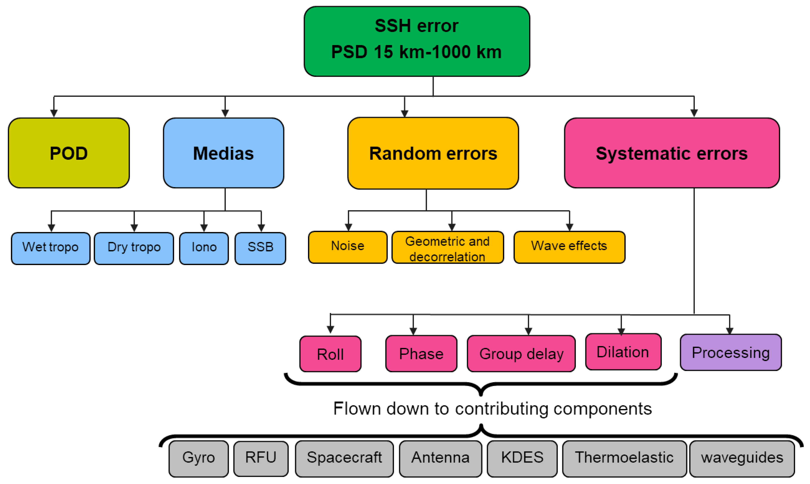
1.1. SWOT Error Budget and Systematic Errors

The Surface Water and Ocean Topography (SWOT) mission from NASA (National Aeronautics and Space Administration), CNES (Centre National d’Etudes Spatiales), CSA (Canadian Space Agency) and UKSA (United Kingdom Space Agency) will provide two-dimensional topography information over the oceans and inland freshwater bodies. Morrow et al. [1] and Fu and Rodriguez [2] give an updated description of the mission objectives, the instrument principle, and the scientific requirements.
SWOT has two main objectives: to observe mesoscale to sub-mesoscale over the oceans and to observe the water cycle over land. To achieve these goals, SWOT’s main instrument is the Ka-band radar interferometer (KaRIn), a synthetic aperture radar interferometer with two thin ribbon-shaped swaths of 50 km each. The other instruments onboard include a Jason-class nadir-looking altimeter (for cross-comparisons with KaRIn, calibration, and nadir coverage), a two-beam microwave radiometer (to correct for the wet troposphere path delay), and a precise orbit determination payload (required for the radial accuracy of topography measurements).
The SWOT mission will fly on two different orbits. The first has a one-day revisit time with very sparse coverage. The one-day orbit will be used for approximately six months during the commissioning phase of the mission. For this reason, it is sometimes called the Calibration/Validation (or Cal/Val) orbit. The second orbit, also called “science orbit”, has a 21-day revisit time with global coverage for latitudes below 78°.
The mission and performance error budget from Esteban-Fernandez et al. [3] highlights the stringent requirements in terms of error control:
  • SWOT’s error budget is required to be one order of magnitude below the ocean signal for wavelengths ranging from 15 to 1000 km (expressed as a power spectrum);
  • KaRIn’s white noise must be less than 1.4 cm for 2 km pixels on ocean (or 2.7 cm for 1 km pixels);
  • KaRIn measurement must have a 10 cm height accuracy and a 1.7 cm/1 km slope accuracy over 10 km of river flow distance (for river widths greater than 100 m);
  • The topography requirements for the nadir altimeter are derived from Jason-class missions.
Among the many error sources described in [3], this paper focused on the so-called systematic errors. These errors have multiple sources, as shown Figure 1: an error in the attitude knowledge (e.g., imperfect roll angle used in the interferogram to topography reconstruction); an error in the interferometric phase or group delay (e.g., from hardware or electronics); an imperfect knowledge of the true KaRIn mast length… The details of each error source are largely beyond the scope of this manuscript and properly addressed by Esteban-Fernandez et al. [3]. Similarly, the breakdown of each error type into sub-system allocations (grey boxes of Figure 1) is not relevant in the context of this paper. However, Figure 1 remains interesting because it gives a good idea of the complexity of the so-called systematic errors.
For practical purposes, the systematic errors in pink can be divided into four signatures or components (more details in Section 2.2): one bias for each swath, a linear component in the cross-track direction and for each swath, a quadratic component common to both swaths, and a residual that is almost constant in time. These four components are independent and additive with other sources of error.
The first three components are shown in Figure 2. While their general form is known analytically, they have a time-varying amplitude, and the amplitude may change at different time scales (e.g., qualitative difference between panel (a) and panel (b)). Moreover, even the so-called ‘bias’ term of panel (e), is only constant in the cross-track direction for a given time step and a given swath (left or right). The value of the cross-track bias may evolve in time, at different time scales, and independently for each swath. The amplitude and the time scales involved are discussed in Section 2.2. We will see in Section 2 that a dedicated calibration algorithm is needed to mitigate these three components, and to keep the overall SWOT error within its requirements.
The last component (or residual) cannot be modeled with a simple analytical model as it contains the sum of complex effects. On the bright side, the residual is mostly time-invariant (see [3]), and it is not ambiguous with the other components (e.g., zero-mean, no linear or quadratic signature). The residual is absorbed by a specific ground correction named the phase screen. To that extent, we will not discuss it here. This paper focuses on the error signatures of Figure 2.

1.2. Data-Driven Calibration

Past papers have explored various mechanisms to mitigate the systematic errors. Enjolras et al. [4] was the first and most simple implementation of the crossover algorithm used for SWOT’s roll error. Dibarboure et al. [5] extended this strategy to resolve other components, as well as more challenging time variations. Furthermore, Dibarboure et Ubelmann [6] explored the strengths and weaknesses of four different types of calibration algorithms, as well as the impact of the satellite orbit and revisit time. Using a similar algorithm on their hydrologic target of interest (Lake Baikal), Du et al. [7] have demonstrated an ability to complement the ocean-based correction presented in this paper with their regional calibration. More recently, Febvre et al. [8] explored the possibility of tackling the same problem with a framework based on physics-informed artificial intelligence.
All these papers use a common approach: they take the KaRIn topography measurement, and they adjust empirical models to isolate the systematic errors. In other words, they are data-driven calibration algorithms. The other common trait of these papers is that they explored the strengths and weaknesses of their algorithm in a vacuum: realistic SWOT errors were not known at the time, let alone simulated by the Project. To that extent, their analyses were useful to understand some concepts and generic implications, but they did not test an end-to-end calibration scheme, nor did they discuss the nature of residual systematic errors after their data-driven calibration.

1.3. Objective of This Paper

In that context, the objective of this paper was to give the first end-to-end overview of the SWOT data-driven calibration problem: why a calibration is helpful or needed, what will be the end-to-end algorithm sequence, and what is the current performance assessment based on pre-launch simulations. This paper briefly summarized the main findings from previous work, but did not duplicate their detailed description of each algorithm (e.g., equations, strengths and limits). Note that the final implementation by the Project will also be documented in the so-called Algorithm and Theoretical Basis Documents (or ATBD) which will be made public soon (no reference at the time of this writing).
This paper is organized as follows. Section 2 details the input data (e.g., ocean models, SWOT orbits, KaRIn noise) and prelaunch scenarios for SWOT (e.g., description of the uncalibrated errors). Section 3 presents the data-driven calibration methodology and the complete algorithm sequence. Section 4 gives the results with the pre-launch error performance (residual error after the calibration is applied), and Section 5 discusses various implications and extensions of this paper, such as sensitivity tests, limitations, and tentative algorithm improvements, as well as a post-launch outlook.

2. Input Data and Prelaunch Scenarios for SWOT

2.1. Input Data

All the simulations presented hereafter started from two simulated datasets (see schematics from Figure 3). Firstly, we generated a simulated SWOT ocean product (nadir altimeter and KaRIn) without the systematic errors (yellow box in Figure 3). Secondly, we generated a simulation of the uncalibrated systematic errors only (blue box in Figure 3) by combining some inputs and data from the SWOT Project. The sum of these contributions yielded a simulated SWOT product before the data-driven algorithm. This input was then injected into the algorithms of Section 3 (red box in Figure 3) to produce a simulation of the calibrated product. By comparing the uncalibrated error simulation (input) with the calibration parameters (output), we can infer the performance of the calibration algorithm.
To simulate SWOT measurements (available in [9]), we used the open-source SWOT Ocean Science Simulator, initially developed by Gaultier et al. [10] and updated by Gaultier et Ubelmann [11]. This simulator first interpolates the surface topography snapshots of an ocean model to emulate a “perfect” SWOT-like measurement of the ocean topography (hereafter considered as our simulated ground truth): nadir altimeter and KaRIn interferometer.
In our study, we used two global ocean models (B1 in the green box from Figure 3):
  • The GLORYS 1/12° model from Lellouche et al. [12], as it is the state-of-art operational system operated by Mercator Ocean International in the frame of the operational Copernicus Marine Service. This global model has a sufficient resolution to resolve large- and medium-mesoscale and is quite realistic when it comes to the global ocean circulation, including in polar regions. However, its relatively coarse resolution makes it unable to resolve small- to sub-mesoscale. Moreover, it does not have any forcing from tides, so the GLORYS topography does not contain any signature from internal tides.
For these reasons, our GLORYS-based simulated SWOT products were considered here as a “best-case” simulation. To illustrate, for actual flight data from SWOT, tides were removed from the topography measurement using a good-but-not-perfect tides model. In the GLORYS simulation, the lack of tidal signature is equivalent to assuming that the tides correction of flight data from SWOT will be perfect (i.e., absolutely zero residual from barotropic and baroclinic tides). Similarly, the lack of small- to submesoscale in our calibration is admittedly optimistic as we underestimate how they might affect our calibration (discussed in Section 5.2.1);
  • The Massachusetts Institute of Technology general circulation model (MITgcm) on a 1/48-degree nominal Latitude/Longitude-Cap horizontal grid (LLC4320). This is one of the latest iterations of the model initially presented by Marshall et al. [13] and discussed in Rocha et al. [14] among others. The strength of this model is the unprecedented resolution (horizontal and vertical) for a global simulation, which makes it possible to resolve small to sub-mesoscale features in the global surface topography snapshots. It is also forced with tides, thus adding important ocean features of interest for SWOT scientific objectives, and as well as more challenges for the data-driven calibration of KaRIn products (see Section 3.3).
However, the LLC4320 simulation suffers from forcing errors on tides (Arbic et al. [15]), resulting in tidal features that might be stronger than reality, as well as forcing errors on the atmosphere (6-h lag resulting in desynchronization of some diurnal and semi-diurnal barotropic signatures). There are also unrealistic behaviors in polar sea-ice and rare spurious data in coastal regions (because of the sea-ice and bathymetry/shoreline masks). Despite these issues, the LLC4320 MITgcm simulation remains one of the best global models we could use in this work. Because of the errors, the LLC4320-based simulated SWOT products are considered as a “worst case” ocean for our calibration study. The forcing errors leave higher residuals, which would be equivalent to very imperfect tides corrections in flight data from SWOT, especially on internal tides;
  • We also used the NEMO-eNATL60 regional model simulation of the North Atlantic at 1/60° from the Institut des Geosciences et de l’Environnement (IGE). Brodeau et al. [16] describe the configuration and the validation performed on this model. Despite its relatively limited geographical coverage (North Atlantic), this model complements our simulations because the topography snapshots compare extremely well with the observations at all scales (i.e., arguably more realistic than the global models above). The model also exists with and without tides, which is very useful to understand the impact of barotropic and baroclinic tides in our local inversions. For the sake of concision, we did not detail the analyses performed with this model as they were generally used to confirm or to modulate some findings from the global models.
Regarding the non-systematic error simulations, we used the default configuration of the SWOT simulator (detailed in [10]). The uncorrelated random noise is generated consistently with the description from the SWOT Project [3], using snapshots of the WaveWatch-III wave model to modulate the noise variance as a function of the significant wave height. The wet troposphere error was generated using the methodology of Ubelmann et al. [17]. The “systematic errors” (namely roll, phase, baseline, timing) were processed separately (Section 2.2).
We also simulated two sets of SWOT products for each ocean model (B2 in the blue box from Figure 3): one set for the 21-day science orbit (the orbit parameters where provided by the SWOT Project. The geometry simulation was performed with the SWOT Scientific Simulator), and one set for the one-day Cal/Val orbit. Having this parallel setup was shown (Dibarboure et Ubelmann [6]) to be very important because the orbit controls the space/time distribution of the SWOT measurements as well as the location and time difference of image-to-image overlaps which are used in our algorithm. This property is shown by Figure 4, where panel (a) shows the very sparse coverage of the one-day CalVal orbit. For this orbit, the entire cycle yields only 10 crossover diamonds per pass (half-orbit) and only two crossovers from 63°S to 63°N. In other words, for this orbit, there are ocean segments up to 6500 km without any crossover diamond. This property will be discussed in the following sections. In contrast, the map of panel (b) and the zoom in panel (c) show that the 21-day orbit has a very dense coverage, where crossover diamonds between ascending and descending passes are nearly ubiquitous (approximately 60,000 crossovers per 21-day cycle).
The consequences of this sampling difference between the two orbits are discussed by Dibarboure et Ubelmann [6] as it defines the types of calibration algorithms that can be used. We will see in the next section that it is the reason why we developed two algorithms: the SWOT-only Level-2 algorithm based on crossover diamonds for the 21-day orbit and for hydrology products, and the multi-mission Level-3 algorithm for the ocean and the one-day orbit.
Note that for both orbits, multi-mission crossovers (e.g., when the Sentinel-3 or Sentinel-6 altimeters are in the KaRIn swath) yield millions of kilometers of 1D crossover segments at all latitudes. Dibarboure et Ubelmann [6] showed that even if we limit these 1D crossovers to short time differences (1–3 h), and two external altimeters, multi-mission crossovers already provide a very good coverage. Adding all other altimeters in operations (e.g., CRYOSAT-2, SARAL, HAYANG-2B/2C, Jason-3 or CFOSAT) yields a massive amount of additional reference points, which can be used as independent measurements of the “ground truth” for data-driven calibration. However, the nadir constellation is limited by the intrinsic noise level of conventional altimeters (i.e., wavelengths larger than 40 km for recent sensors to 70 km for older altimeters).

2.2. Uncalibrated Error Scenarios

To simulate the uncalibrated systematic errors, we developed two reference scenarios with the SWOT Project (B3 in the blue box from Figure 3). The first scenario was based on the spectral allocations of Esteban-Fernandez [3]: for each component, we considered that 100% of the spectral allocation is an actual error (i.e., no margin with respect to allocations). We used an inverse FFT on the reference spectra provided by the SWOT Project, and we generated a one-year realization in the temporal domain (i.e., a time-evolving signal with the right along-track correlation). We repeated the process for each component of Figure 1.
In practice, the following additive cross-track components are generated:
  • A bias in each swath originating in the group delay of either antenna (timing error);
  • A linear signature in each swath originating in the interferometric phase error;
  • A linear signature in both swaths originating in imperfect roll angle knowledge (e.g., gyrometer error);
  • A quadratic signature originating in the imperfect knowledge of the interferometric baseline length.
Because each of these spectra follows a K−2 power law: the power spectrum S decreases as the wavenumber k increases with the relationship S(k) ∝ k−2. The PSD is therefore linear with a slope of −2 in a log/log plot. The resulting error contains a continuous mix of large amplitude and low-frequency errors, and smaller amplitude and higher-frequency errors (e.g., a mix of Figure 2a,b). This “allocation” scenario is now the default configuration of the SWOT simulator [11]. In the context of data-driven calibration, we consider this allocation scenario as a worst-case (or pessimistic) because each component is at the acceptable limit given in the breakdown of the SWOT error budget.
In contrast, the second scenario used the most recent simulations from the Project, in order to get closer to the expected performance at launch (i.e., lower error because the Project has margins for each component). The second scenario is the “current best estimate” (or CBE) pre-launch error assessment from the SWOT Project. It was first setup in 2017, then revised in 2021 (hence the label CBE21) using more faithful simulations and hardware test outputs. In comparison with the allocations of the first pessimistic scenario, the uncalibrated errors can be smaller by a factor of 2 to 10 for some components and wavelengths.
However, these simulations might arguably underestimate some error sources, or simply not replicate unknown effects that will be discovered on flight data. To that extent, this CBE21 scenario should be considered as optimistic in the context of our data-driven calibration assessment. To use a consistent wording with the first scenario, we will hereafter talk about CBE21 as our best case scenario even though it is not strictly optimal for each error component. To summarize, one might expect the reality of flight-data calibration errors to be higher than our CBE21 scenario and lower than the allocation scenario.
Furthermore, for the CBE21, we use the sum of two simulations provided by the SWOT Project: one simulation for the attitude knowledge error (essentially errors from the star-trackers and platform, attitude reconstruction algorithm), and one simulation for the KaRIn instrument (thermo-elastical distortion of the antennas or mast, thermal snaps, electronics…). Both simulations use a common value for the beta angle that is shown in Figure 5. This angle, between the sun and the SWOT orbit plane, is important as it controls the thermal conditions along the orbit circle (e.g., eclipses) for the platform, attitude sensors, instrument structure, electronics, etc.
In addition to the two simulations from the SWOT Project, the random error originating in the precise gyrometer was simulated as it was in the allocation scenario: inverse FFT of the roll spectrum to replicate the random nature of this error. The spectrum itself is robust and based on flight-proven performance from previous missions: the K−2 spectrum is the integration in time of the gyrometer white noise on angular velocities.
Figure 6 gives an overview of the simulated attitude knowledge error. Each curve in panel (a) shows the roll knowledge error (in arcsec) made along two subsequent revolutions, and the induced topography error (in cm RMS). The colors correspond to the first revolution of each day over a 21-day cycle (and all beta angle configurations). The general shape of these curves shows that the error is dominated by a non-zero mean value up to 10 arcsec (i.e., 2 m RMS on KaRIn topography) and a smooth signal that can be approximated by a handful of harmonics and sub-harmonics of the orbital period (repeating patterns). The amplitude along the orbit circle ranges from 5 cm to tens of centimeters. The mean value and the harmonics also change continuously each day: this change is controlled by the beta angle from Figure 5. This modulation is more visible in Figure 6b, which shows the roll error as a function of time throughout one year. The peaks in this panel correspond to the phases when the beta angle goes to zero (the sun is in the orbit plane). On top of this slowly evolving signal, each transition in and out of eclipse is simulated by the SWOT Project with a transient signature of a few minutes and a small amplitude (e.g., Figure 6c) to approximate the response to thermal snaps. The final output of this first simulation is shown in Figure 6d.
The second simulation used as an input for our study is for the KaRIn instrument. Our input data was generated by the structural thermal optical (STOP) simulator, which is used by the Project to perform end-to-end analyses of in-flight temperatures and deformations of external structures. This simulator reproduces many complex effects and error sources that are beyond the scope of this manuscript.
As far as data-driven calibration is concerned, Figure 7 gives an overview of the latest iteration of the STOP simulation (updated in 2021). In practice, the total simulated STOP21 error is essentially the sum of three components: a bias for each swath, a linear cross-track component for each swath, and a quadratic cross-track component. There is also a residual with a centimeter-level mean value (to be tackled by the Phase Screen algorithm) and a sub-millimeter evolution around the mean. By construction, this residual is not corrected by our algorithm, so it will be a small contributor to the error after our calibration.
Panel (a) of Figure 7 shows the temporal evolution of the bias root mean square error (RMSE) over one year (top figure) and a zoom over the first 11 h. Panels (b) and (c) are the same for the linear and quadratic components. These figures illustrate very well the order of magnitude of the topography signature, as well as the four time-scales involved:
  • There is a large non-zero mean for this one-year simulation. In practice, this yearly average might exhibit small inter-annual variations. To illustrate, the Sun controls the illumination and thermal conditions of the satellite. The Sun also has an 11-year cycle. This solar cycle might show up in SWOT as very slowly evolving conditions. In other words, our “non-zero mean” could actually be found to be a very slow signal from the natural variability of the Sun. This yearly time-scale indicates that any calibration performed on a temporal window of one 21-day cycle or less should yield a non-zero mean;
  • Slow variations with time-scales of the order of a few weeks to a few months. These modulations are caused by changes in the beta angle of Figure 5. Note that the relationship with the beta-angle can be quite complex, hence the need of a sophisticated simulation such as STOP21. This time-scale indicates that any calibration performed on a temporal window of a few hours or less will observe a linear evolution of the uncalibrated errors;
  • Repeating patterns with a time-scale of the order of 15 min to 2 h. These signatures are clearly harmonics of the orbital revolution period (e.g., thermal conditions changing along the orbit circle in a cyclic pattern). This time-scale indicates that the calibration algorithm can exploit the repeating nature of some error signatures using orbital harmonic interpolators rather than basic 1D interpolators;
  • High-frequency components with a time-scale of a few minutes or less (essentially high-frequency noise or sharp discontinuities in the curves of Figure 7). These high-frequency components are also broadband because they are affecting many along-track wavelengths (as opposed to the harmonics of the repeating patterns). This time scale is important because it might affect the ocean error budget (requirement from 15 to 1000 km, i.e., 2.5–150 s), either globally if the error is ubiquitous, or locally at certain latitudes if the high-frequency error is limited to specific positions along the orbit circle.
Furthermore, Table 1 gives an overview of the error RMS for each component and for each time scale. These values should be compared to the SWOT hydrology requirement and error budget. The total requirement is 10 cm RMS, and the primary contributor is the allocation for systematic errors (7.5 cm RMS). Table 1 shows that many components are much larger than this requirement. That is the reason why a data-driven calibration is required for SWOT to meet its hydrology requirement. The rationale is clearly explained in the SWOT error description document from Esteban-Fernandez [3].
For oceanography, the requirements are articulated as a 1D (along-track) power spectral density (PSD) from 15 to 1000 km. The last column of Table 1 shows that, for these scales, SWOT does not need a calibration algorithm to meet its ocean requirements, the content of STOP21 is below its spectral allocation for all wavelengths from 15 to 1000 km (not shown), and even significantly below for most components. To that extent, the STOP21 simulation confirmed the statements from Esteban-Fernandez [3].
Nevertheless, because the presence of low frequency bias/linear/quadratic signals would leave decimetric to metric residual errors in the cross-track direction (i.e., alter 2D derivatives such as geostrophic velocities, vorticity, etc.), it would be quite beneficial to apply a data-driven calibration of ocean products as well. Such an ocean calibration should be focused only on wavelengths larger than 1000 km, in order not to alter the SWOT products in the critical wavelength range of 15 to 1000 km where requirements apply.
To summarize, in the sections below, we use two “uncalibrated error” scenarios (B3 in Figure 3). The spectral “allocation” scenario is our pessimistic/worst case, which assumes that each systematic error source is set to 100% of its theoretical allocation. The “current best estimate 2021” scenario is a more realistic (arguably optimistic/best case) simulation input that was built with the SWOT Project. The uncalibrated errors can be as large as a few meters (two orders of magnitude larger than the SWOT requirements) and they have four different time- scales: inter-annual, beta angle variations, orbital harmonics, and periods shorter than 3 min (approximately 1000 km).
The data-driven algorithm aims to reduce the three systematic error components (bias, linear, quadratic) in each swath, and for time scales ranging from the 3 min to slower components. This is required to meet the hydrology requirements of 7.5 cm RMS (the calibrated error must be smaller than this threshold). Over the ocean, no calibration is required to meet the 1D along-track spectral requirements from 15 to 1000 km, but a data-driven calibration would be beneficial to reduce the metric-level cross-track errors and biases originating, especially for time-scales longer than 3 min where the amplitude is large.

3. Method: Data-Driven Calibration and Practical Implementation

This section gives an overview of the data-driven calibration algorithms. They are used on the input data of Section 2 to generate the results of Section 4. In Section 3.1, we first make a brief synthesis of the calibration principles detailed in previous papers [4,5,6], and we recall the main pitfall of such empirical algorithms, then we present two end-to-end calibration schemes (B4 in the red box from Figure 3). The first algorithm (Section 3.2) is a part of the operational SWOT ground segment (Level-2): its goal is to ensure that hydrology requirements are met in a robust and self-sufficient way (SWOT data only). The second algorithm (Section 3.3) is a research counterpart that is operated in a multi-mission context (Level-3): its goal is to further improve the performance over the ocean, and in the very specific case of the one-day orbit.

3.1. Data-Driven Calibration: Basic Principles

All data-driven calibration algorithms share the same basic principle. The systematic error sources have a signature on the measurements of water surface topography that is known analytically. Therefore, it is possible to adjust an analytical model on the measured topography, and to remove it, using just the SWOT topography product. This is why the algorithm is often called empirical, or data-driven.
To illustrate, the roll error creates a linear signature in the cross-track direction. The simplest way to remove the error would be to adjust a linear model in the cross-track direction for a given time step, or for a given time range. By repeating the process for each time step, and by removing the adjusted value, any signature from roll would be effectively removed. This basic strategy is called the “direct” retrieval method in [6]. Note that it can be used wherever the KaRIn image is almost complete (few missing/invalid pixels). In other words, it can be used almost everywhere over the ocean and large lakes. However, it cannot be used over most inland segments: the KaRIn topography will be usable only in the presence of inland water (rivers, reservoirs, floodplains…), which results in extremely sparse inland coverage: not enough to use a data-driven calibration.
The pitfall of this data-driven approach is that KaRIn has a very narrow field of view (2 × 50 km with a near nadir gap of 2 × 10 km). At these scales, the actual geophysical slope (ocean and inland waters) is not zero. There is an ambiguity between the systematic errors and the true topography of interest: the two signatures are by no means numerically orthogonal. As a result, a poorly implemented algorithm would alter, or even destroy entirely some signals of interest. The same effect would happen in the presence of geophysical errors on KaRIn data: wet troposphere path-delay residuals left by an imperfect radiometer correction, sea-state bias with a cross-track signature… Dibarboure et Ubelmann [6] extensively discuss this so-called leakage of geophysical signatures in the calibration algorithms.
The actual challenge of the data-driven calibration is therefore not to remove the errors, but to isolate them from the signal of interest. To achieve this goal, it is necessary to orthogonalize the numerical problem, i.e., to leverage some properties of the signal and errors so that they become less ambiguous. In practice, Dibarboure et Ubelmann [6] describe and discuss three different methods to achieve a better separation:
  • M1: One can use a first guess or prior for the true ocean topography (or sea surface height, SSH). The rationale is to remove as much ocean variability as possible with external data, in order to reduce the ambiguity with the systematic errors.
The first step is to not use the SSH, but to remove a mean sea surface (MSS) to cancel out the geoid and the mean dynamic topography (MDT). Similarly, instead of the raw sea surface height SSH, it is very important to apply all geophysical corrections and to use a corrected SSH anomaly (SSHA). To illustrate, by removing a model for the barotropic tides, we remove most of the ambiguity between this geophysical content of the SSH, and the systematic errors, which mitigates the leakage of tides into the calibration.
The second step is to reduce the influence of the ocean circulation and mesoscale. To do this, mono-mission algorithms can build a first-guess (or prior) from the SWOT nadir altimeter (M1a). Similarly, multi-mission algorithms can leverage higher-resolution topography maps derived from the nadir altimeter constellation (M1b), or even topography forecasts from operational ocean models;
  • M2: One can use image-to-image differences instead of a single KaRIn product. When the time lag between two images is shorter than correlation time scales of the ocean, using a difference between two pixels will cancel out a fraction of the ocean variability (the slow components). The closer in time the two images are, the more variability is removed with this process.
Furthermore, the residual ocean variability that remains in the image-to-image difference is not only smaller in amplitude, but also shorter in spatial scales. Because the field of view of SWOT is only 120 km from swath edge to swath edge, having smaller geophysical features means we improve the orthogonality between the errors and ocean.
In practice, Dibarboure et Ubelmann [6] describe three algorithms based on this differential strategy. The first method (M2a) is based on crossover differences: when an ascending pass and a descending pass meet, there is a diamond-shaped region where they overlap. This algorithm can be used for all orbits, but when the orbit revisit time of 21-day or more; most of the SWOT coverage is actually within a crossover diamond (see Figure 4c). In contrast, for the one-day orbit, there are only 10 crossovers per pass, and they can be thousands of kilometers away from one another (see Figure 4a). For the one-day orbit, the SWOT mission will revisit exactly the same pixels every day. So, it becomes possible to perform an image-to-image difference everywhere. Leveraging this property of the one-day orbit is the basis of the collinear retrieval algorithm (M2b) from [6].
The third differential strategy is the sub-cycle algorithm (M2c): it was developed for a backup orbit option of SWOT where adjoining swaths are only one day apart from one another (i.e., one-day orbit sub-cycle). Yet, at the time of this writing, SWOT will not use this orbit, so we will not discuss the sub-cycle algorithm here. It is still noteworthy because it might be interesting for future swath-altimeter missions with different orbit properties (see Section 5.5);
  • M3: One can use a statistical knowledge of the problem to reduce the ambiguity. Qualitatively, most ocean features look very different from a 1000+ km bias between the left/right swaths of KaRIn, or a quadratic shape aligned with the satellite tracks, or the thin stripes of high-frequency systematic errors. From a numerical point of view, the 3D ocean decorrelation scales in space and time are very different from the covariance of swath-aligned systematic errors. Similarly, the SWOT errors have an along-track/temporal spectrum which is known from theory, hardware testing. It can also be measured from uncalibrated data (see Section 5.4). It is therefore possible to replace simple least square inversions by Gauss-Markov inversions or Kalman filters that exploit this statistical information. This was shown by [6] to reduce significantly the leakage of the ocean variability into the calibration parameters. The process can be used either during the local retrieval (M3a) such as in a crossover region, or it can be used to better interpolate between subsequent calibration zones (M3b).
The calibration model adjustment is performed in so-called “calibration zones”. For various reasons, these zones are not ubiquitous. There can be gaps between them (e.g., between subsequent crossovers in Figure 4c). Conversely, when multiple algorithms are used, the calibration zones of two methods can overlap. To that extent, one needs to interpolate/blend the local calibration estimates into a unique and global calibration dataset.
Consequently, the overall calibration is organized as in the schematics of Figure 8. There is a three-step process. Step 0 removes as much geophysical content as possible from KaRIn measurements (e.g., large mesoscale) using an ocean prior or first-guess. At the end of step 0, only the high-frequency, high-wavenumber ocean features remain in the calibration input. Step 1 activates one or two local calibration retrieval methods on KaRIn images, or on image-to-image differences. At the end of step 1, we collect a series of calibration models per error component (bias, linear quadratic) in so-called calibration zones (e.g., crossover diamond) with an uncertainty (e.g., error covariance). Then step 3 performs the final fusion of the local calibration models into a global calibration that can be applied to reduce the systematic errors over any region, surface type, and target. This correction is also provided with an uncertainty (or quality flag).
As discussed above, the leakage mitigation methods M1 to M3 exist in different flavors. This results in two very different algorithm sequences. The blue color in Figure 8 is for the Level-2 algorithm. This sequence is designed for the SWOT ground segment: it secures the hydrology error requirements; it must be based on SWOT data only (KaRIn + nadir) to ensure that the mission is self-sufficient; and it must be resilient to inaccurate pre-launch assumptions (e.g., it cannot be affected by incorrect spectra or decorrelation functions). In contrast, the red color is for the Level-3 algorithm. This sequence is operated in a multi-mission and non-operational context so it can leverage as many external datasets as needed. It is also designed as a research processor so it can use more sophisticated but fragile variants with 3D covariance functions and in-flight measured spectra. The Level-2 sequence is detailed in Section 3.2; and the Level-3 algorithm is detailed in Section 3.3. Their output performances are described in Section 4.1 and Section 4.2, respectively.

3.2. Ground Segment Calibration Algorithm Sequence (Level-2)

This algorithm sequence uses the blue boxes of Figure 8. In processing step 0, we use the nadir altimeter content as a prior of the sea surface height anomaly (SSHA). In processing step 1, we use the direct method to calibrate the bias in each swath, and the crossover method for the other components (linear and quadratic). The image-to-image difference is computed for crossover regions, and the linear and quadratic models are adjusted on the difference. This results in a series of local calibration models for each component. Then in processing step 2, we inject these local models in an orbital harmonics interpolator to retrieve the repeating patterns along the orbit circle. Lastly, we interpolate the residual with a simple kernel interpolator (least squares, weighted with each error bar, Gaussian kernel, 1000 km cut-off). Because the interpolator sometimes encounters some extremely long segments as long as 10,000 to 20,000 km, the interpolator switches to linear interpolation when the kernel is smaller than the distance between subsequent crossovers.
Figure 9a shows an example of the uncalibrated error (linear component) for one arbitrary revolution. Panel (a) shows its overall geometry: the revolution starts in the South Pacific, crosses the ocean up to North America, then it goes through Greenland, Europe and Africa. Then it crosses the Indian Ocean and Southern Ocean, and it ends over Antarctica. Figure 9b shows, as a function of time, the evolution of the uncalibrated error (linear component): the blue dots are for the ocean, and the red ones for the inland segments. As expected from the spectral allocation scenario (K−2 power law), the error contains a mix of large-scale and large-amplitude features, and rapid changes with a smaller amplitude. In addition to the curve of panel (b), this revolution is also affected by a very large signal from the attitude knowledge error (e.g., Figure 6a) that is a nearly perfect sine function at the orbital revolution period.
Figure 10 shows the step-by-step inversion for an arbitrary crossover region. Panel (a) is the starting point and final objective (to retrieve this simulated ground truth). Adding the systematic errors in panel (b) completely skews the KaRIn images by tens of centimeters. By forming the crossover difference on the overlapping diamond (panels c and d), we can then use the residual as the input for a least square inversion. In the inversion, we adjust the bias, linear and quadratic analytical models for each swath and each pass. By construction, the least squares minimize the residual variance in panel (e). If we apply the local calibration model, we observe in panel (f) that we correct most of the input errors: near the crossover, the retrieved SSH matches the simulated ground truth of panel (a). The algorithm properly isolated the systematic error signatures from the signal of interest.
Furthermore, the crossover diamonds are nearly ubiquitous for the 21-day orbit. This is shown by the darker regions of Figure 4c, and quantified in ([6], Figure 17). In practice for the example revolution of Figure 9, we obtain the dense crossover coverage of Figure 11a. For each crossover region, we get an estimate of each component of the systematic error. For the Level-2 algorithm, each crossover yields only a scalar value and a scalar uncertainty for each component. For the Level-3 algorithm below, the same inversion can yield a 1D segment instead of a scalar, and a covariance error instead of a scalar uncertainty.
The local crossover model is then injected in the interpolation processing step (Figure 11). For the Level-2 algorithm, we use two subsequent interpolations. Firstly, we correct for the massive (up to 5 m) orbital harmonics and constant signals using an interpolator with sine-functions and frequencies set on multiples of the orbital revolution period (hereafter orbital harmonic interpolator). Because the latitude coverage of ocean regions is very different from pass to pass, we compute the harmonics interpolation over a window of 4 revolutions (eight passes) in order to ensure that all latitudes are observed for ascending and descending crossover segments. This parameter is a trade-off between the performance (a larger time window yields better results) and the practical constraints of operating the algorithm in the ground segment (see Section 5.2.3). The result of this sub-step is shown in panel (b): the input crossover points are the pink dots with a vertical error bar, the estimated harmonics is the red curve, which approximates the true error (black/blue curve) very well. Once the harmonic interpolation has been performed, only the broadband residual remains. It is mitigated by the second interpolator (Figure 11c).
To mitigate the broadband signal, we use the Gaussian interpolator (also known as Gaussian smoother) that both interpolates and low-pass filters a global correction (black line) from the crossovers (green dots with their vertical error bar). The resulting residual (thin grey line) is very small in comparison with the uncalibrated broadband error (blue/red dots). Over the ocean (blue dots in panel c), the interpolator can retrieve even rapid changes in the uncalibrated error, but it is sometimes misled by imperfect crossovers (e.g., leakage of ocean variability, coastal crossovers, sea-ice region…). In contrast, the performance over land is dominated by the lack of local calibration zones (only ocean crossovers can be inverted). As a result, the error increases when KaRIn gets further away from the ocean.

3.3. Research Calibration Algorithm Sequence (Level-3)

This algorithm sequence uses the red boxes of Figure 8. This sequence was initially designed for the one-day orbit, and more specifically because of the very sparse crossover coverage discussed in Section 3.1. Indeed, we will see in the next section that the Level-2 algorithm might not be able to meet the hydrology requirements for this orbit in worst-case scenarios.
The main strength of the Level-3 algorithm sequence is that it is operated in a multi-mission and non-operational context so it can leverage as many external datasets as needed (e.g., mitigation method M1b). It is also designed as a research processor so it can use more sophisticated but fragile variants that exploit covariance functions and in-flight measured spectra as well as to combine crossovers with other retrieval methods (e.g., to merge M2a and M2b) in a “statistically optimal” interpolator (mitigation methods M3a and M3b). Because of this, the Level-3 sequence is well suited to improve the calibration over the ocean, as opposed to the Level-2 algorithm, which only focuses on inland hydrology requirements. Furthermore, the Level-2 algorithm is designed not to affect the small ocean scales (as discussed in Section 2.2, ocean requirements from 15 to 1000 km are met without data-driven calibration). In contrast, the Level-3 is not bound by the limits of the ground segment, thus it can try to reduce the error even for wavelengths smaller than 1000 km.
Like in the Level-2 sequence, processing step 0 uses a prior to reduce the amount of ocean variability (barotropic signals or mesoscale) before the calibration itself. However, in the Level-3, our prior combines the nadir altimeter of SWOT, with a similar content from all other altimeters in operations. The process used to merge the altimeter datasets was developed by Le Traon et al. and Bretherton [18,19]. In their analysis of multi-altimeter maps, Ballarotta et al. [20] illustrate that such a prior captures most of the large mesoscale variance (e.g., wavelengths of 130 km in the Mediterranean Sea or 200 km at mid-latitudes). In practice, our mapping algorithm is a variant of the operational algorithm described by Dibarboure et al. [21]. The two specificities of our prior are that:
1/The coverage is limited to the location and time of KaRIn data (not a global map of SSHA). This choice makes it possible to retrieve smaller and faster features that are often smoothed out in global maps;
2/The local mean is defined by the nadir altimeter from SWOT in an effort to isolate the data-driven calibration of KaRIn’s systematic errors (which by definition affect KaRIn only) from all other sources of errors and ocean variability (which also affect SWOT’s nadir altimeter).
Processing step 1 is then to operate three of the four inversion schemes described by Dibarboure et Ubelmann [6]: for the 21-day orbit, we combine the direct retrieval method and the Crossover retrieval Method, and for the one-day orbit we combine the direct method and the collinear Method.
As discussed in Section 3.1, the advantage of the direct method is its simplicity and universality (it requires a single KaRIn image). So, this method can be used everywhere, on all orbits. The downside is that it is prone to leakage from ocean variability in the correction (the M1 prior is never perfect). In the Level-3 sequence, the leakage is mitigated because we use covariance functions (mitigation method M3a) to reduce the ambiguity between the topographic signatures of the systematic errors and the ocean. This approach is extensively discussed in [6].
Nevertheless, Figure 12 shows that a small residual leakage remains. The black line in panel (a) is the uncalibrated roll error that the direct method is trying to retrieve. This KaRIn segment is located in the North Atlantic (panel b). This particular segment has a mean value of 2.5 arcsec (i.e., the KaRIn image is tilted by tens of cm) with slow variations (1000–5000 km) of about 1 arcsec, and rapid changes approximately an order of magnitude below (i.e., a few centimeters). The colored lines are the calibration outputs of the direct method when using different ocean priors: a flat surface (yellow), a barotropic tides model (purple), tides plus a static mean dynamic topography or MDT (green). These priors were tested because they are compatible with Level-2 limitations. A common feature to all these simulations is that the direct method is well centered on the mean value, and that the large-scale roll errors are properly retrieved. However, these examples illustrate quite well the limit of using such static priors: when the KaRIn image is in the Gulf Stream, the retrieved roll value in yellow/purple/green clearly deviates from the true uncalibrated value. This is because the scale and magnitude of the ocean eddy slopes is so large that they are misinterpreted as roll signatures in the KaRIn image. In other words, ocean variability leaks into the calibration, as described by [6].
Conversely, the effect is strongly attenuated when we use a Level-3 implementation where the ocean prior is built with a multi-nadir map (red line). The red line (retrieved roll in Level-3) is very close to the black one (uncalibrated true roll error) even in the presence of the largest eddies. This example illustrates the benefits of using mitigation methods M1b: with a better prior, we mitigate the leakage of ocean variability the calibration. The data-driven calibration is now accurate even in the presence of large ocean eddies (i.e., a few hundreds of kilometers).
Yet at smaller scales, the right-hand side part of Figure 12a still exhibits high-frequency deviations from the black line for all colored lines. This calibration error also originates in the leakage from ocean features into the calibration, but not from mesoscale variability. Indeed, the zooms in Figure 12c,d show that the high-frequency calibration artifact actually originates in the presence of very large internal tide (IT) stripes in the KaRIn image. In the MITgcm snapshots, the internal tides have an amplitude of 5 cm or more in the Tropical region, and because of their orientation, there is a non-zero cross-track slope component. Furthermore, these signatures are different from mesoscale eddies so even using mesoscale covariance functions in the Direct retrieval method does not help to lift the ambiguity between this signature and actual roll. As a result, the IT signature leaks into the calibration and the output deviates from the black line with the repeating pattern of IT (here almost a plane wave). Figure 12 uses roll as an example for the sake of clarity, but the same phenomenon occurs on other calibration models (bias and quadratic).
One may argue that the MITgcm ocean reality used in the simulation is known to have some errors in the tides forcing [15], and therefore that this example is much worse than what will happen in reality. Nevertheless, this example still clearly illustrates the existence of an undesirable phenomenon: internal tides might be a significant source of calibration error in many regions. It also illustrates that the direct method has intrinsic limitations because we use a single thin ribbon-shaped image. Generally, the direct method works quite well for wavelength longer than 300 to 500 km. Below this value, the KaRIn field of view of 2 × 50 km makes it very hard to isolate systematic errors from ocean signals.
Indeed, Figure 13 shows that in a KaRIn swath, the presence of MITgcm internal tides often creates apparent slopes over the 120 km swath. These slopes have a temporal repeating pattern of 12 and 24 h, as expected. Because of the interactions between internal tides and ocean mesoscale, the topography signature is modulated with time scales of the order of 7 to 15 days (e.g., Ponte and Klein [22]). In turn, this property can be leveraged by the crossover and collinear algorithms: by using an image-to-image difference with a time difference of 1 to 10 days, a fraction of the topography signature is cancelled out when the 2 images are in phase with tides. Because the one-day orbit has a revisit time of almost 24 h, the internal tide signature is almost the same in subsequent KaRIn images, like in the left and right panel of Figure 13a. Other ocean features might change a little, and interact with the internal tides, but the bulk of the internal tide topography signature gets removed in a difference of subsequent daily revisits.
Furthermore, at these scales, the dominating systematic error have random sources. In other words, they change with each sample. There is no repeating pattern at these short wavelengths, so the uncalibrated errors do not cancel out in the image-to-image difference. This property makes it possible to leverage the collinear Method or Crossover Method to mitigate the ocean leakage (IT and medium mesoscale) during the inversion.
In contrast, for large-scale systematic errors (e.g., more than a few thousands of kilometers), there is a repeating pattern clearly visible in the samples of Figure 7. Because they are repeating, these large-scale errors get cancelled out in a day-to-day difference, so they will not be mitigated by the collinear Method. In other words, this retrieval method is less efficient for scales larger than a few thousands of kilometers. It is necessary to use both the collinear and Direct method concurrently: the former is used to reduce the influence of internal tides and large mesoscale, and the latter is used to retrieve large-scale repeating patterns.
That is where the processing step 2 of Figure 8 comes in. Firstly, we blend the larger scales of the Direct retrieval and the smaller scales of the collinear retrieval. This can be done by summing the outputs of a robust and simple low/high-pass filter, or by using a ‘statistically optimal’ interpolator (Gauss-Markov or Kalman) where we setup the error covariance models of each input. The blended solution, also known as ‘hybrid’ retrieval combines the best properties of each algorithm. The rest of the interpolation is the same as for the Level-2: first, we use a harmonic interpolator with the orbital revolution sub-harmonics like in Figure 11b, then we interpolate the residual to provide a ubiquitous correction like in Figure 11c.
The result is shown in Figure 14. In contrast with the accuracy of the direct method (green line), the collinear Method (blue line) is clearly biased, and generally bad for larger scales. However, using the day-to-day difference strongly reduced the high-frequency signatures of internal tides in the right-hand side part of the plot: the collinear retrieval yields higher precision and lower accuracy. Combining both retrievals into a Hybrid solution (red line) gives the best results: a good retrieval of the large scales and mean, and a strong reduction of the high-frequency errors from the green to the red line.
For the 21-day orbit, we cannot use the collinear retrieval method because the revisit time is too long when compared with the ocean decorrelation scales or the internal tide demodulation scales of Figure 13b. However, we can use a similar approach with the Crossover Method. The difference is that the local/solar time of the ascending and descending images is not always aligned with the tidal frequencies, so we cancel out a smaller fraction of the internal tide signal.
Note that for Level-2 algorithms, the crossover inversion yields a single scalar for each model (linear, quadratic, and bias per swath) using least squares: the algorithm is more robust and still enough to meet hydrology requirements. For Level-3 algorithm where we try to provide better ocean calibration, we can also retrieve intra-crossover variations of the error and we can leverage the 2D covariance models like in [5].
To summarize, the Level-3 algorithm sequence is a three-step process (red boxes of Figure 8). Step 0 is to use the nadir altimeter constellation (SWOT nadir + Sentinel-6 + Sentinel-3A/3B) as a prior for the large mesoscale. Step 1 is to activate two data-driven retrieval methods for each orbit (Direct + collinear for the one-day orbit, Direct + Crossover for the 21-day orbit). Step 2 is to blend the two retrievals using a Gauss-Markov interpolator, then to interpolate orbital harmonics, and lastly to interpolate the residual in order to have a global correction for the ocean and for hydrology.
The impact of using inaccurate covariance models in Level-3 algorithms was discussed in [6]: the retrieval is not much sensitive to an incorrect level of variance (e.g., regional variations), but the correlation scales are more impactful. In other words, this Level-3 algorithm sequence requires a good statistical knowledge of the correlation models (i.e., the slope of the power spectra). It is relatively easy to setup in simulations as we can perfectly characterize the input fields (ocean and uncalibrated errors). However, in real life, it requires an accurate estimation of the uncalibrated errors of flight data (discussed in Section 5.4) as well as a good statistical description of the true ocean (hence our sensitivity tests with different ocean models, see Section 5.2).

4. Results: Prelaunch Performance Assessment

Section 3 gave a general description of the data-driven calibration algorithms, and it described the two algorithm sequences we implemented (mono-mission Level-2 and multi-mission Level-3). In this section, we present the simulation results and the data-driven calibration performance. Section 4.1 focuses on the Level-2 algorithm sequence, i.e., the calibration sequence implemented in the pre-launch ground segment of SWOT. Section 4.2 then tackles the Level-3 performance, i.e., the expected performance of a research-grade offline correction.

4.1. Performance of Level-2 Operational Calibration

4.1.1. SWOT’s 21-Day Orbit

The maps from Figure 15 show the residual error when the Level-2 data-driven calibration is applied over a one-year period. The left panels are for the 21-day orbit: panel (a) is for the spectral allocation scenario, and panel (c) is for the CBE21 scenario (see Section 2.2). The former is arguably a pessimistic or worst case, and the latter might be the most faithful pre-launch simulation.
The maps clearly show two different regimes: ocean and land. Over the ocean, the error after calibration is low with 2 to 3.5 cm for the ‘spectral allocations’ in panel (a) and less than 2 cm for CBE21 in panel (c). Higher errors are observed in sea-ice regions because sea-ice crossovers cannot be used in the data-driven calibration (sea-ice covered regions are actually processed like inland segments). The ocean error is also higher in western boundary currents and the Antarctic Circumpolar Current (ACC). The higher residual is created by the leakage of ocean variability into the correction. Note that the extra error variance in these regions -of the order of a few cm2− is very small in comparison with the regional SSHA variability, which can be one or two orders of magnitude larger. In other words, only 1% to 5% of the ocean signals leak into the calibration.
For hydrology, the error is much larger. For panel (a), it ranges from 4 cm RMS in coastal regions or small continents (Greenland or Australia) to more than 10 cm RMS at the heart of larger continents (North and South America, Africa and Eurasia). For the CBE21 scenario in panel (c) the error ranges from 3 to 7 cm RMS with a very similar geographical distribution. The error naturally increases as SWOT gets away from the ocean because the calibration is made using ocean data, and then interpolated over land. So the farther away from the last ocean crossover, the larger the interpolation error RMS. This is important because depending on where the hydrology target is located, the error level of the Level-2 product could almost triple.
Moreover, in addition to the continent-scale geographical variability, there is also a smaller scale variability associated with the swath width. Indeed, because most of the error are linear or quadratic-shaped in the cross-track direction, the RMSE is higher on the outer edges of the KaRIn coverage. An example is given in Figure 16d where the center of the swath has a 5 to 7 cm RMSE whereas the error on the outer edges can be as large as 8 to 10 cm if not more. To that extent, it is quite important to know where a hydrology target is located within the swath, especially for the one-day orbit where a given point is seen by only a single KaRIn pass.
In addition to the geographical variability, there is also a significant amount of temporal variability in many regions. Indeed, Figure 16 (panels a and b) shows the same maps as Figure 15a, with data from opposite seasons. In North America or Eurasia, the error can be three times larger during the wintertime (Figure 16a) than during the summertime (Figure 16b). The opposite is true over Antarctica and the Southern Ocean. In contrast, other regions have a relatively stable error level (e.g., Australia, South America, Africa, most of the ocean). The reason for this temporal variability is given by Figure 16c: most SWOT passes that go through the northern continents also go through the Arctic Ocean where the seasonal sea-ice coverage strongly affects the crossover coverage. During the wintertime, extremely few crossovers can be used. This results in extremely long interpolations starting from the Indian Ocean coast, Eurasia, the Eastern Siberian Sea or Beaufort Sea, then North America and up to the North Atlantic coast. That is almost an entire hemisphere or 20,000 km without any ocean crossover.
In contrast, during the summertime, the Arctic Ocean gets free of sea-ice, and it becomes possible to have at least a handful of crossovers between Eurasia and North America, which essentially cuts the long interpolation into two smaller ones. Furthermore, as expected from the uncalibrated error power spectra (K−2 power laws), the error rapidly increases with the interpolated segment length. The process is also shown analytically by Esteban-Fernandez in [3]. The longer interpolations created by sea ice induce larger error residuals.
For Antarctica, the same process occurs with the sea-ice coverage of the Southern Ocean. During the southern wintertime, the Antarctica segments are longer because of the presence of sea-ice around the continent, and the interpolator error increases as well. While the process over Antarctica has a smaller magnitude than in the Northern hemisphere, the error increase over the Southern Ocean is very large (local error multiplied by 2.5 or 3). This is why even 1-year simulations exhibit significantly higher errors in the regions where sea-ice may appear during the wintertime.
Furthermore, Table 2 (row 1 and row 3) gives an overview of the global root mean square error (RMSE) for both surfaces and for each scenario. Over the ocean, the error ranges from 1.5 cm RMS for CBE21 to 2.2 cm RMS for the spectral allocations. For inland segments, the error is 3.1 cm RMS for CBE21 and 6.5 cm RMS for spectral allocations. In both cases, the residual error after calibration is less than the SWOT hydrology requirements, and the right-hand side column gives the margins with respect to these requirements (between 25% and 83%). In other words, in our simulations, the Level-2 algorithm is actually able to successfully reduce the systematic errors by 1 or 2 order of magnitudes, as well as to meet the hydrology requirements at global scale.
Nonetheless, there is a significant amount of geographical and seasonal variability. For the CBE21 scenario, the requirements are met in all regions and all seasons. For the scenario with spectral allocation however, there is much more variance left, and in particular in the 5000 to 15,000 km range where sea-ice affects the interpolation process. As a result, the error after calibration can be locally higher than the requirements, in particular during the wintertime and the Northern hemisphere.

4.1.2. SWOT’s One-Day Orbit

The right-hand side panels from Figure 15 show the residual error when the Level-2 data-driven calibration is applied for the one-day orbit. Panel (b) is for the spectral allocation scenario and panel (d) is for the CBE21. The continents, these maps are somewhat similar to panel (a) and (c) for inland regions. The farther away from the ocean, the higher the residual error after calibration. The error is also larger in many regions such as South America or Antarctica.
In contrast, the geographical distribution over the oceans is very different panel (a) and panel (c). The residual error was quite homogeneous for the 21-day orbit and increasing only because of ocean variability. For the one-day orbit, the error is still 2 to 3 cm near the ocean crossovers, but these crossovers are so sparse, and so far away from one another, that very long interpolations must be performed between them. As a result, the ocean error strongly increases in all ocean regions that are far from ocean crossovers: to illustrate, near the Equator the error can be as large as 7 cm RMS, i.e., more than one order of magnitude higher in variance (or power spectrum). This major change in crossover distribution is also the reason why the inland error is higher for the one-day orbit. For a given river or lake, the closest ocean calibration zone is sometimes much farther away with sparse one-day crossovers than for the denser crossover coverage of the 21-day orbit. As a result, the inland interpolated segments are usually longer, sometimes by more than 5000 km. And like in the presence of sea-ice discussed above, longer inland interpolations yield larger calibration errors.
The values of Table 2 for the one-day orbit (row 2 and row 4) show that the ocean global RMSE increases at lot for the allocation scenario, which in turns increases the inland RMSE. The result is that the hydrology requirements are no longer met for the one-day orbit (the margin becomes minus 8%). In contrast, for the CBE21 scenario, the error increases much less over the ocean (from 1.5 to 2 cm RMS) which, in turn, barely affects the inland RMS and margins. For this CBE21 scenario, there is significantly much less uncalibrated variance in the STOP21 simulations than in the allocations for wavelengths above 5000 km, which in turns reduces not only the total error, but also the necessity to have crossovers at all latitudes and all regions.
To summarize, the one-day orbit becomes a more challenging problem for the simple and robust Level-2 algorithms. One the one hand, the official CBE21 scenario from the SWOT Project indicates that the algorithm is enough to meet the requirements. On the other hand, the pessimistic/worst case spectral allocations indicate that if flight data suffer from a larger uncalibrated error, the Level-2 algorithm might be insufficient to meet the hydrology requirement during this phase. This finding was one important driver for the definition of the Level-3 algorithm.

4.1.3. Spectral Metrics

As explained in previous sections, the ocean requirements are expressed as power spectra density (PSD) thresholds from 15 to 1000 km. In essence, the total SWOT error budget must always be below a small fraction the ocean SSHA spectrum (SNR = 10 dB) for these wavelengths. This will ensure that KaRIn captures correctly at least 90% of the variance of large to small mesoscale, or even submesoscale features. It also ensures that the spectral slopes of interest for oceanographic research are not significantly affected by measurement errors.
Figure 17a shows the PSD of the ocean requirements in red (extended up to 10,000 km), the uncalibrated error in black. From 15 to 1000 km, the uncalibrated error allocation is significantly below the requirements. As discussed in previous sections, data-driven calibration is not needed for SWOT to meet its ocean requirements.
The blue line in Figure 17a (error PSD after Level-2 calibration) shows that the crossover algorithm starts to kick in at 1000 km: the blue line departs from the black line, i.e., the calibration is effectively mitigating the errors. This is by construction as we estimate only one scalar value per crossover in processing step 1 and the Gaussian interpolator of processing step 2 is setup to smooth scales smaller than 1000 km. For scales smaller than 1000 km, the data-driven Level-2 calibration leaves the data untouched since the requirements are met anyway. Above 1000 km, the calibration reduces the error by a factor 2 to 50: the longer the wavelength, the better the error reduction. There is also (not shown) a huge gain at the orbital revolution period (40,000 km) because a lot of uncalibrated error variance is concentrated near this specific frequency (see Section 2.2).
However, in the case of the CBE21 in the 21-day orbit (Figure 17b), the uncalibrated error (black) is almost an order of magnitude below the allocation for all scales, especially above 1000 km. Because the magnitude of the uncalibrated is smaller, the crossover algorithm kicks in at 2500 km where it removes as much as 30% of variance for the larger scales. In the CBE21 scenario, the data-driven calibration essentially removes only the variance of the orbital harmonics and for very large scales. This is the reason why it is less affected by the sparse crossover coverage in Figure 15d. In contrast, Figure 17c shows that for the allocation scenario of the one-day orbit, and despite the large amount of uncalibrated variance from 1000 to 10,000 km, the Level-2 crossover method is barely efficient below 5000 km. This is a spectral view of the higher errors in Figure 15b when KaRIn is away from crossovers.
Note that we defined the 1000 km limit with SWOT’s Project Team. The rationale is to not alter the data if the raw measurement already meets the requirement. However, the practical consequence is that the residual error after calibration could be as large as 5 cm RMS and more for the one-day orbit. This choice is the second driver for the definition of the Level-3 algorithm: to provide the best possible ocean calibration for scales above and below 1000 km for both orbits.

4.2. Performance of Level-3 Research Calibration

As shown in Section 3 and Figure 12, the main difference between the Level-2 and Level-3 algorithm is that the multi-altimeter prior makes it possible to use the direct retrieval method. Furthermore, the crossover implementation is different: using the 2D covariance functions makes it possible to resolve the intra-crossover variability in addition to the scalar values of Level-2 as per [5]. Furthermore, the interpolation step 2 can make a statistically optimal use of each retrieval method (e.g., large scale of direct, less internal tides in collinear) including below 1000 km.
The positive impact of these changes is shown in the green and purple spectra of Figure 17. Indeed, the Level-2 algorithm kicked in near 1000 km (panel a, 21-day orbit) to 5000 km (1-day orbit). In contrast, the Level-3 algorithm is now beneficial from 400 km for the allocation scenario to 700 km for the CBE21 scenario. The gain from Level-2 to Level-3 calibration ranges from a factor of 2 to 5 below 1000 km, to a factor of 20 or more for 5000 km and above.
This is due to the Direct and collinear retrieval Methods and the multi-altimeter prior. Because we use a single KaRIn image instead of sporadic crossovers, the retrieval is possible everywhere: it is no longer necessary to have a good ocean crossover nearby. Furthermore, Figure 17 shows the difference between the direct retrieval only (green spectra) and the Hybrid retrieval (purple spectra), which blends the direct with collinear or Crossover Methods. At global scale, the gain is significant but arguably limited (30 to 50% of variance for wavelengths ranging from 250 to 2000 km). However, the benefit can be significantly more in specific regions (example from Figure 14).
More importantly, Figure 17b,c show that the Level-3 spectral performance is essentially the same for these two very different simulations (CBE21 and allocations, 21-day and one-day orbit). This is explained by the findings of Dibarboure and Ubelmann [5]: over the ocean, the limiting factor is (by far) the ocean variability leaking into the correction (unchanged between Figure 17b,c). In other words, the accuracy of the prior used in processing step 0 essentially controls the Level-3 calibration performance.
Furthermore, the maps from Figure 18a, and Figure 18c show that the geographical distribution of the error is the same as for Level-2. For the ocean, the error clearly increases with ocean variability and in the presence sea-ice. The effect is more pronounced than for the Level-2 algorithm for two reasons: (1) the background RMSE for the direct/hybrid retrieval is much lower than in Figure 15, and (2) our blending method is not yet statistically optimal (the error bar associated with the ocean leakage of the direct method is not properly setup). For hydrology, the inland interpolator remains the dominating source of error, hence an error increase from coastal regions to large continents.
From a statistical point of view, Table 3 shows the RMSE for the global ocean and for inland segments as well as the improvement with respect to the Level-2 figures of Table 2. For the 21-day orbit, the global ocean is improved by 60% of variance and the residual error after calibration is at centimeter level. Like in the spectra from Figure 17, the performance is essentially the same for the CBE21 and ‘spectral allocation’ scenarios (the limiting factor is ocean leakage and SWOT’s narrow field of view). Because the inland performance is dominated by the interpolator error, the gain for hydrology is significant but smaller (10–20%) in the case of the 21-day orbit. The gain for hydrology originates in a better interpolation setup in the coastal ocean, and a lower reliance on specific crossovers located in key regions (e.g., semi-enclosed seas).
In contrast, the results for the one-day orbit are quite different from the Level-2 performance reported in Section 4.1.2. The Level-3 algorithm is no longer limited by the crossover coverage: the direct and collinear retrievals can be used everywhere. As a result, the data-driven calibration behaves in a similar way for both orbits. This results in a variance reduction of 80 to 95% for the global ocean. The gain is also clearly visible in the difference between the blue and green/purple spectra of Figure 17c: the gain can be as large as two orders of magnitude for the larger scales (which also contain the bulk of the error variance), and the calibration starts to be effective from 400 km and above (as opposed to 5000 km for the Level 2).
Lastly, because the ocean is better calibrated, the improvement is also visible inland with a gain of 20 to 40% with respect to the Level-2 algorithm. The Level-3 residual error of the same for both orbits. Although the inland interpolators are still affected by the presence of sea-ice in the Arctic, the Level-3 algorithm is not strongly limited by the very sparse crossover coverage of the one-day orbit at low to mid-latitudes. In the Level-2 algorithm, this sparsity would increase the length of the interpolated inland segments by thousands of kilometers. With the Level-3 algorithm, the ocean retrieval is always as close to the coast as numerically possible whether there is a crossover or not.
More importantly, even in the worst scenario (spectral allocations), the residual error after calibration remains at 6 cm, i.e., within the hydrology requirements with good margins (30% of signal variance). In other words, if flight data have an error closer to our ‘pessimistic’ scenario than the Project’s CBE21 scenario, the Level-3 research algorithm might still be able to provide a beneficial correction for offline product reprocessing.

4.3. Summary of Results

We have successfully implemented the complete data-driven algorithm sequences presented in Section 3, and evaluated their performance (i.e., the systematic error residual after calibration) in simulations using 16 pre-launch scenarios from the SWOT Project (see Section 2.2). An important set-up with respect to previous work was the realism of the uncalibrated errors at global scale, and more importantly, the higher fidelity of the ocean models used to simulate the true ocean.
The Level-2 algorithm was developed for the SWOT ground segment and to meet the hydrology requirements (global RMSE of 7.5 cm for inland segments). It yields a mean inland error of 3 to 6 cm, i.e., margins of 25–80% of the signal variance. For hydrology, the main source of residual error is the long inland interpolations between ocean crossovers. This results in geographically variable performance where long inland arcs (e.g., Eurasia to North America) yield higher residuals than short inland segments (e.g., Europe or Australia). Because the Arctic Sea is frozen in winter, there is also a significant temporal variability of the residual errors after calibration.
Over the ocean, the Level-2 residual error is approximately 2 cm for SWOT’s 21-day orbit. By design, the Level-2 calibration only affects scales above 1000 km where it reduces the errors by a factor of 5–20. In contrast, the calibration has no effect below 1000 km, nor on the SWOT ocean science requirements (PSD from 15 to 1000 km). This is expected since the uncalibrated systematic error is already within this requirement: the ocean error budget is secured by the instrument stability and payload design.
Furthermore, for the first six months, SWOT will use a one-day revisit orbit with very few crossovers (hundreds of times less than with the 21-day orbit). As a result, the Level-2 algorithm yields acceptable results only in our optimistic CBE21 scenarios (6.5 cm RMSE or 25% margins for hydrology, 3 cm RMSE for the ocean). However, in our pessimistic/worst case scenario, its performance is insufficient for both hydrology (requirement not met by 8%) and oceanography (5 cm RMSE after calibration).
The Level-3 performance assessment in prelaunch simulations shows a significant step-up with respect to the results of the operational Level-2 algorithms. For hydrology, the gain ranges from 20 to 40% for the 21-day orbit where the Level-2 was already quite efficient. In addition, for the one-day orbit, even our worst-case scenario yields a residual error less than 6 cm, i.e., good margins with respect to the requirements. Furthermore, the Level-3 is particularly attractive for the ocean, which was not the focus of the Level-2 algorithm. Indeed, the Level-3 algorithm yields a residual error of the order of 1 cm RMS for all orbits and input scenarios, i.e., an error variance reduction of 60 to 90% with respect to the Level-2 algorithm used by the ground segment. The Level-3 algorithm is also able to reduce systematic errors down to wavelengths as small as 400 km, i.e., beyond the mission requirements. More importantly, the Level-3 algorithm has a more stable performance as it does not rely on crossover coverage, which is very sparse for the one-day orbit.
However, the Level-3 algorithm is also more fragile as it relies on external measurements from the nadir constellation, and a good setup of the 2D covariance models, which might be challenging for flight data: in particular, our simulations already exhibit a significant amount of leakage of the ocean variability in some regions (more than with the Level-2 crossover retrieval). To that extent, the Level-3 algorithm is not (yet) compatible with the constraints of an operational ground segment. Once qualified and optimized with flight data, this might change in the future.

5. Discussions

The methodology and results presented in previous sections raise a series of questions discussed in the sections below. Section 5.1 describes the differences between offline and near real time performance. Section 5.2 discusses the sensitivity of our results to various simulation inputs (ocean models and uncalibrated error). Section 5.3 discusses the main algorithm limitations and tentative improvements. Section 5.4 explains how this pre-launch work will be validated and updated with flight data. Lastly, Section 5.5 extrapolates our findings to future swath-altimeter missions.

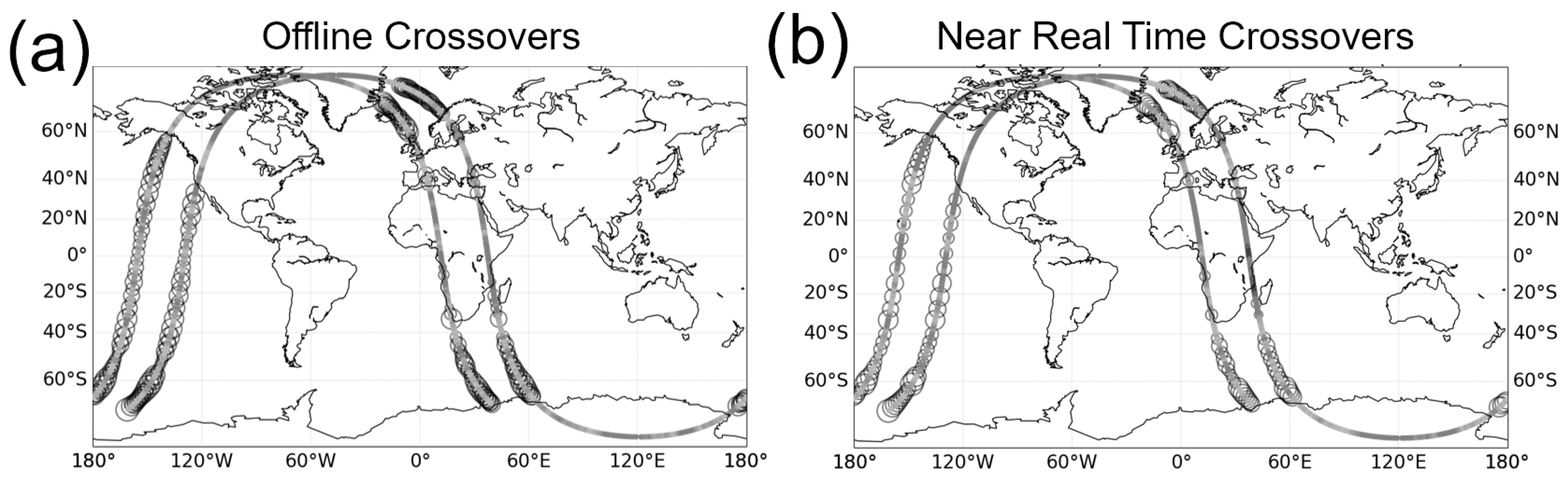
5.1. Near-Real Time Performance

The performance assessment presented in Section 4 uses offline or delayed-time (DT) simulations. In other words, when we calibrate a given KaRIn product (time-tagged t0), we use data from its past (e.g., time-tagged t0 minus 10 days), and data from its future (e.g., time-tagged t0 plus 10 days). However, if the algorithm is operated in near-real time (NRT), it becomes impossible, by definition, to use future measurements: they have not yet been collected by KaRIn. This statement is relevant for the three processing steps of Figure 8.
Firstly, near-real time constraints affect the quality of the nadir-altimeter prior used in processing step 0: in our simulations, the ocean prior map has the accuracy of an offline altimeter map, which is better than a near-real-time one. The difference of quality between NRT and DT maps was first discussed by Pascual et al. [23]. They showed that the error of gridded altimetry products could increase by up to 30% in near-real time. Dibarboure et al. [24] then showed that adding real time along-track products and more altimeters could reduce the NRT-specific error to a much smaller fraction (typically less than 5%). To that extent, we did not replicate the very complex behavior of the operational nadir-altimeter systems. We can assume that a lower performance of the multi-mission prior will affect the accuracy of the direct retrieval method by an equivalent 5% since the dominating source of error is mesoscale leakage.
Secondly, near-real time limitations affect the crossovers in processing step 1: in delayed time, we can form crossovers between a given product at t0 and other passes located up to t0 + 10 days. In contrast, for near-real time, it becomes impossible to form such crossovers, and we can form only crossovers with older products. As a result, the number of crossovers is essentially divided by a factor of two. In a vacuum, this would be a significant concern for the Level-2 algorithm. Indeed, we have seen in Section 3.2 that losing crossover coverage can strongly affect the overall performance when the crossover coverage is already sparse (e.g., Arctic in wintertime or one-day orbit).
However, in practice, the NRT limitation have a relatively low impact thanks to the properties of the SWOT orbits: any 21-day KaRIn coverage is made of two interleaved and homogeneous grids from subsequent sub-cycles of 10 days each. When the algorithm is operated in near real time, the processing time window is [t0 − 10 days; t0] instead of the nominal offline time window of [t0 − 10 days; t0 + 10 days]. Consequently, we actually lose an entire sub-cycle grid. Moreover, because the sub-cycle grid from future is well interleaved with the crossover grid from past data, the crossover coverage is strongly reduced, but it is still very homogeneous from a geographical point of view. Operating the algorithm in near real time does not create a massive aggregation of missing crossover in specific regions (which might happen with a different orbit).
This is illustrated in Figure 19, where the crossover coverage of delayed time (panel a) and near-real time (panel b) clearly differ in the quantity of crossovers (as expected, half of them are missing in panel b), but the remaining crossovers in NRT are actually interleaved with the decimated ones. Consequently, the calibration over the ocean still benefits from a decent retrieval: the crossovers missing in NRT are not aggregated in specific regions where a very long interpolation would be needed like for the one-day orbit. And for hydrology, some coastal crossovers might be lost, but the ocean constraint is still evenly distributed. Consequently, the inland interpolation is slightly longer in NRT than in DT, but the NRT crossover loss does not create a massive data gap like in the Arctic during the wintertime. In our NRT simulations, we observe an increase of the RMSE that ranges from a few percent for most regions to 15% wherever the crossover coverage is already sparse.
Lastly, near-real time limitations affect the interpolators of processing step 2. In offline mode, the interpolator always has a buffer of future data when processing a given product or day. In other words, the product/half-revolution to calibrate is always at the center of the processing time window. In contrast, for near-real time, the processing time window must be offset and stopped at the last product. In practice, the SWOT ground segment activates the algorithm once per day with a timeliness of a couple of days. In other words, the interpolator problem becomes marginal except at the very end of a KaRIn product, i.e., in polar regions covered by sea or land ice (i.e., no performance requirement). Even for those regions, the effect is quite rare because the SWOT ground segment operates the data-driven calibration sequence on a daily basis: only one pass over 28 is affected, i.e., 3% of the data in polar regions.
To summarize, in near real time, the RMSE after calibration increases by less than 5% for the Level-3 algorithm (because of the low quality of the NRT nadir-altimeter prior), and less than 15% for the 21-day orbit Level-2 algorithm (i.e., largely covered by our margins to meet the hydrology requirements). Based on the margins reported in Section 4, there is no performance issue to operate the calibration algorithm in near real time.

5.2. Sensitivity to the Simulation Inputs

Because the pre-launch simulations highly depend on the quality and realism of the input data, we performed various sensitivity tests to verify that our findings were robust. We also explored some stress cases to understand what would happen in case of unexpected discoveries on flight data: SWOT is the first of its kind and we cannot rule out unexpected findings on small ocean mesoscale, their interaction with internal tides or surface waves, or unexpected measurement errors. Lastly, we performed a series of stress tests against major data gaps and routine mission events (e.g., the 180° yaw flip periodically made by the satellite, orbit maintenance maneuvers) to test the algorithm robustness against the inevitable operational data gaps.

5.2.1. Simulated Ocean Reality

As far as the ocean model is concerned, we confirmed that the end-to-end algorithm sequence exhibits the same type of sensitivities reported by Dibarboure and Ubelmann [6] in their limited experiments. The ocean variability leakage is the primary source of error over the ocean. Therefore, to obtain a realistic error assessment, it is essential to use a simulated ocean from a very high-resolution model that features not only the largest eddies but also a good fraction of the energy cascade, interactions between internal waves and sharp gradients, etc. Using a lower resolution model results in artificially good performance because the ocean leakage is largely underestimated.
Similarly, it is essential to have a good sea-ice mask, as it controls the areas where the ocean calibration can or cannot be performed. As shown in Figure 16, the seasonality of sea-ice coverage is a strong component of the final error assessment. Using a perfect ocean model without a sea-ice mask would result a very large underestimation of the inland interpolation error because the simulations would not include the very long wintertime interpolations (with higher errors) of Figure 16c.
To a lower extent, it is better to use a model with realistic internal tides as they contribute to the leakage. However, having realistic tides in the simulated ocean is essential only when trying to design the best ocean calibration algorithm (i.e., less than 2 cm RMSE, lower error spectra from 100 to 2000 km). In contrast, we observed that having imperfect barotropic tides or barotropic atmospheric signals in the model topography did not significantly affect our inland results. In other words, using a model without tides will barely affect the hydrology error budget, nor will it affect the outcome of a simple calibration algorithm (e.g., our Level-2 sequence).

5.2.2. Simulated Orbital Harmonics

In the examples from Figure 6 and Figure 7, the SWOT simulations are quite smooth, and the signal can be approximated by very few orbital harmonics. This is because of the stringent design of the instrument and platform. However, one might argue that they are optimistic, and that flight data might prove to be more complex to handle.
To illustrate, Figure 20 shows a recent thermoelastical simulation performed by Thales Alenia Space (personal communication) for the European Space Agency in the frame of Phase A/B1 analyses for the future Sentinel-3 Next Generation altimeters of the Copernicus Program (wide-swath scenario). The blue curve in the upper panels is the uncalibrated roll. This plot is very interesting because it is quite different from SWOT simulations. Indeed, the amplitude is much smaller than for SWOT, but the shape is much more complex: it is clearly not possible to approximate it with a few harmonics because there is a sharp behavior change near 900 and 1900 s (transitions in and out of eclipse). As a result, the model from panel a (the orbital harmonic interpolator from SWOT) is unable to approximate the truth: the roll error after calibration is 0.45 arcsec RMS (i.e., 9 cm RMS).
However, it is possible to adjust the interpolator (processing step 2) to better fit the new input signal. Figure 20b is when we use the same interpolator but adding more harmonics. In this case, the roll RMSE is 0.06 arcsec or 1.2 cm. This is worse than for SWOT but arguably good enough for the global ocean. Still, there might be high-frequency residuals as large as a couple of centimeters when the orange curve locally departs from the blue one. Such residuals would show up as latitude-specific bands on the ascending and/or descending passes. Thus, the next step would be to perform two separate interpolations for the illuminated and eclipse portions of the orbit circle since the transitions are perfectly predictable. In the very crude implementation of Figure 20c, the residual is 0.6 cm RMS, which is almost as good as for our prelaunch SWOT simulations. More sophisticated variants would also better handle the transition and remove the discontinuity for even lower residuals.
This example from a preliminary Phase A study illustrates quite well that some details and parameters of SWOT’s pre-launch algorithm can be adjusted to match the behavior observed on flight data. The adjustment is simple, and the output performance of the modified algorithm is essentially the same as for our pre-launch simulations.

5.2.3. Data Gaps

In our simulations, the SWOT products are always available. There is no missing data, no edited nor spurious data. However, in real life, SWOT products will never be 100% complete. In addition to the existence of spurious pixels (e.g., for nadir altimetry, approximately 4% of the product is unavailable because of quality flags), SWOT products will be periodically unavailable: orbit maneuvers, onboard gyrometer calibration sequences, 180° yaw flip maneuvers, etc. Moreover, during the mission’s lifetime, it is possible if not likely that the nadir altimeter and the KaRIn swath altimeter will be temporarily unavailable (e.g., Single Event Upset, which requires hours or days of expert analysis before the instrument is rebooted). As far as the data-driven calibration is concerned, flight data will therefore be periodically incomplete: data gaps will range from random pixels to entire missing products (data gaps of a few hours to a few weeks).
We tested the robustness of the calibration algorithm against the presence of such (simulated) data gaps. We performed these tests in near-real time conditions, as it is the most difficult configuration for our algorithm. In our experiment, we simulated a data gap of 11 days. Because we stop computing crossovers if the time difference is more than 10 days, this data gap is equivalent to cold-restarting the algorithm, with almost zero input data.
For the first 7 h, there are not enough KaRIn products for the algorithm to work: the crossovers are all located in polar regions, and it is not possible to compute a correction for lower latitudes. With 8 to 11 h of data, the first low latitude crossovers can be formed, and the Level-2 algorithm converges immediately to a good performance (hydrology requirements are met). After less than 24 h, the nominal NRT performance is reached.
This is an interesting finding because it confirms that the Level-2 algorithm is robust. Unless it is operated on almost zero SWOT products (less than 7 h, i.e., 7 passes over 11 days, i.e., 2% availability), it yields a beneficial correction, and with 3.5% of product availability, the performance is almost nominal.
As far as the Level-3 algorithm is concerned, using the direct retrieval method further increases the robustness: crossovers are an optional addition, but the algorithm can be operated with the direct retrieval on a single KaRIn product. In contrast, the collinear algorithm is more affected by the presence of data gaps because it leverages the daily revisit to form image-to-image differences, so a single missing pass would actually affect the same location for the day before and the day after. If we observe that such large data gaps are frequent enough, a logical evolution of the collinear retrieval would be to widen the temporal window to three days or more in order to have backup differential measurements in case of sporadic data gaps.

5.3. Algorithm Limitations and Possible Improvements

5.3.1. Hydrology

Arguably the biggest limitation in the simulated performance for hydrology is the large discrepancy in performance between different continents, regions, and seasons. This variability originates in the long inland interpolations when the river or lake is far away from an ocean crossover. The rationale for this limitation is to have a calibration that is completely independent from the inland water heights, i.e., to have a simple linear processing flow in the ground segment: the ocean processor is activated, the data-driven calibration is activated, and then the hydrology processor uses the ocean-based calibration to activate the hydrology processing.
Nevertheless, it is in theory possible to leverage the good stability of many lakes and reservoirs, as well as instrumented areas where the water height is known without KaRIn. Similarly, KaRIn might be able to measure accurately the height of some fixed targets such as buildings, bridges, or large roads, assuming that they are bright enough. If KaRIn is able to measure such stable targets and if enough of them are located far away from the coast, they might be used as additional reference points for the calibration interpolator (processing step 2) to reduce the interpolation error over large continents. To illustrate, assuming KaRIn retrieves heights with a precision of the order of 20 cm RMS (i.e., twice the SWOT inland error budget) for 20 in-situ points at the center of a given inland segment; then that would roughly equivalent to one reference point of the order of 4.5 cm RMSE. In other words, instead of the current unconstrained interpolator (up to 10 cm RMSE at the center of large continents), the interpolator error would be contained to much lower values for this specific pass. Repeating the process for all passes and large continents, the hydrology error could be significantly lowered. Note that using this strategy would likely be limited to Level-3 offline processors (complexity of the ocean/hydrology sequence, time to collect ancillary data…).
We did not implement this strategy in our pre-launch algorithm for two reasons: (1) the good performance of the pre-launch simulations (large margins reported with respect to the requirements), and (2) we did not have a global simulated dataset for inland waters. Using inland control points is a contingency evolution of the algorithm if flight data prove to be more challenging to calibrate than in our pre-launch simulations.

5.3.2. Ocean

By far the main limitation of the data-driven calibration is the small swath of KaRIn: with only two ribbons of 50 km each, the systematic errors overlap with actual ocean variability. For wavelengths ranging from 50 to 500 km, cross-track topography gradients and quadratic signatures could originate in mesoscale and internal tides. For wavelengths above 1000 to 5000 km, linear signatures and biases could originate in barotropic signals (e.g., tides, inverse barometer).
Unfortunately, the empirical nature of the algorithm makes it weak with respect to such leakage: when the signal and errors are not orthogonal in the inversion space, the ambiguity cannot be resolved. The first way to reduce the leakage is to use ancillary data before the data calibration is used. Consequently, it is important to keep improving various aspect of SWOT’s Level-2 processing: better barotropic tide models, better dynamic atmospheric corrections, better internal tide models, better wet troposphere correction algorithms, mean sea surface models… Similarly, it is important to keep improving gridded multi-mission nadir altimeter products (also known as Level-4) in parallel with swath altimetry. SWOT’s flight data will likely give insights as to the most impactful algorithm improvements for future missions.
Moreover, our simulations show that Level-3 algorithms have more long-term potential once key parameters are properly characterized with flight data (e.g., small-scale ocean decorrelation function, uncalibrated error spectra…). However, their multi-mission nature makes them challenging to implement in a traditional mono-mission ground segment. In the long term, it is likely important for SWOT and for future missions to re-inject Level-3 (or research) corrections into the core Level-2 product. Although it is likely impossible to achieve in near-real time processors, SWOT might demonstrate that this strategy should be at least considered for delayed-time processors and for reprocessing campaigns.

5.4. Validation of Flight Data

We have seen in previous sections that it is quite important to perform an analysis of the systematic errors of flight data: to parameterize Level-3 algorithms, or to demonstrate that requirements are met. A logical strategy would be to use a ground truth (e.g., in-situ measurements, or airborne measurement system) to gauge the accuracy of KaRIn data with and without calibration. However, this strategy has an important limitation.
In situ or airborne observations will be local in space and in time, whereas the SWOT error budget is global. To illustrate, the RMS requirement for hydrology is an average over all hydrology targets above a given size, i.e., all regions and all seasons. As we saw in previous sections, there is a large amount of geographical and temporal variability of the systematic error residual (factor of 3 or more after calibration). If there are only a small number of instrumented rivers and lakes, it is therefore quite difficult to demonstrate that SWOT meets its requirements everywhere else and for different continents and seasons.
For oceanography, the Project must demonstrate that the spectral requirements from 15 to 1000 km are met globally without data-driven calibration, and we need to verify that said calibration does not degrade the content for these wavelengths. Incidentally, we might also want to quantify the benefits of the calibration for larger ocean scales. That spectral requirement might be verified in one or two calibration sites and airborne campaigns, but it is simply impossible to have a reliable ground-truth to verify a global requirement for all ocean dynamics or sea-state conditions.
In the following Section 5.4.1, Section 5.4.2 and Section 5.4.3, we will discuss how we can use additional validation methods to complement the ground truth strategy, and to infer a global performance assessment of KaRIn flight data.

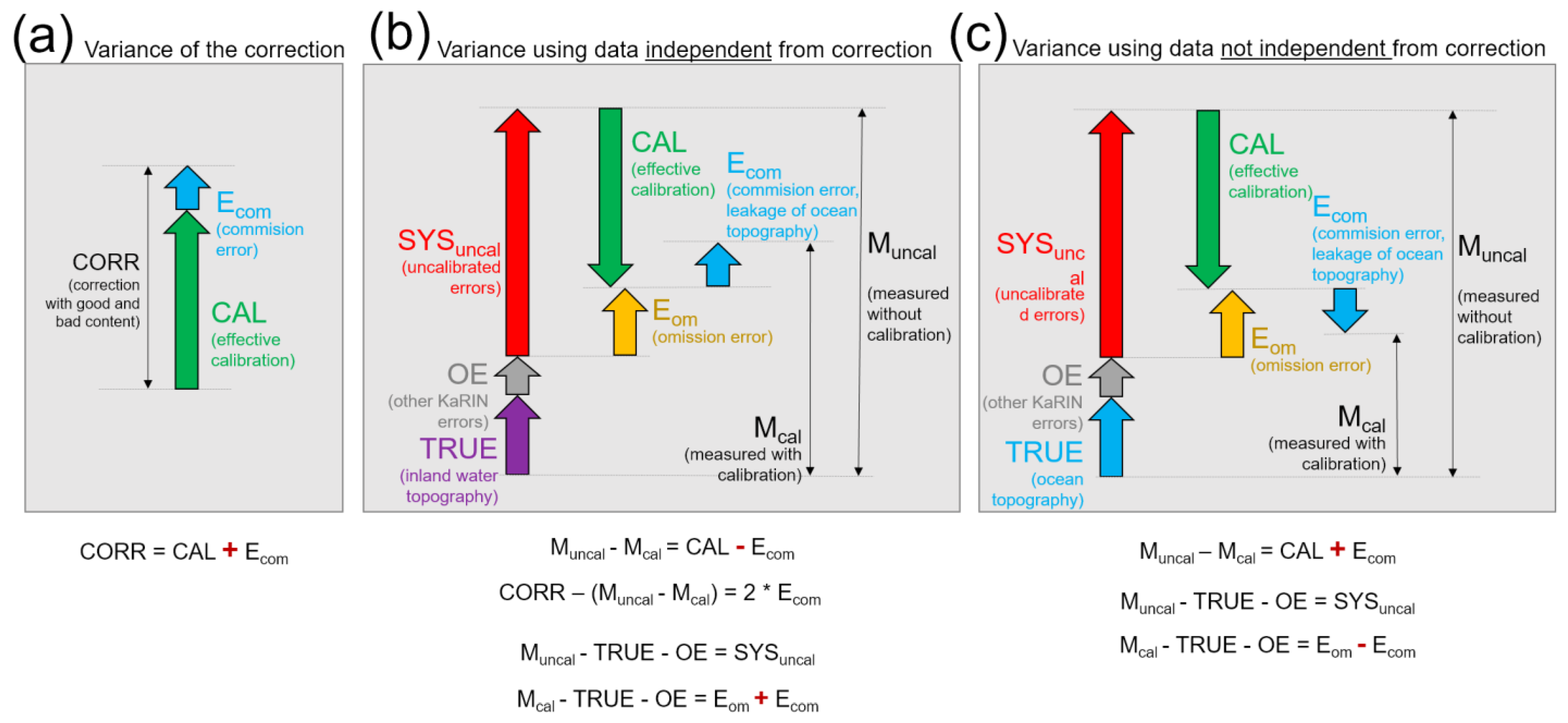
5.4.1. Validation Data: Independent VS. Correlated

It is important to underline that the total systematic error after calibration (i.e., the calibration residual) is the sum of two errors with a very different nature:
  • The commission error (Figure 21a) appears when the calibration introduces new errors from external sources (bad measurements, algorithm error, etc.). In our context, the primary source of commission error would be the leakage from ocean signals, and may be residual wet troposphere error or sea-state bias… In contrast, random noise barely affects the data-driven calibration: in our sensitivity studies, increasing random noise by a factor of 10 in variance, yields almost exactly the same results.
  • The omission error (Figure 21b) appears when the calibration does not have enough measurements to retrieve the signal of interest (i.e., the uncalibrated systematic errors). In our context, the error primarily originates in the interpolation between crossovers or inland.
These errors are quite different. By definition, the former is contained in the data-driven correction applied on KaRIn topography measurements, whereas the other is not. As shown in the schematics of Figure 22a, measuring the variance of the correction yields the sum of the variance of the effective calibration (the content that will actually reduce the systematic errors) and the variance of the commission error. In contrast, the omission error is, by definition, not contained in the variance of the calibration retrieval. Exactly the same logic applies to power spectra instead of variances, and cross-spectra instead of covariances.
Therefore, when we apply the correction on any KaRIn data, the effective calibration content (green arrow in Figure 22) will always reduce the variance of the measured data (the green arrow is downwards in Figure 22b). Similarly, the omission error (yellow arrow in Figure 22) will always behave like an undesirable variance in the calibrated data (yellow arrow is always upwards).
In contrast, the impact of the commission error (blue arrow in Figure 22) will be opposite for the inland and ocean data (Figure 22b,c respectively). Indeed, the calibration is data-driven and derived from ocean data only. For inland data, the natural variability of rivers and lakes or random inland measurements errors are completely independent from the systematic errors and the calibration (i.e., the correlation with them is zero). Thus, when we apply the calibration on inland data, the commission error will actually increase the variance of calibrated data because it cripples the efficiency of the variance reduction from the effective calibration (the blue arrow is upwards in Figure 22b).
For ocean data however, the leakage from actual ocean variability and ocean measurement errors into the correction creates a positive correlation with the correction. So when we apply the correction, the commission error will actually suppress a fraction of the true ocean variability (the fraction that leaked into the calibration). Therefore, in this case, the commission error artificially reduces the variance of calibrated ocean data (the blue arrow is downwards in Figure 22b).

5.4.2. Cross-Spectra Validation Method

Arguably, the most useful tool to perform the analysis is the cross-spectra analysis methodology developed by Ubelmann et al. [25]. This method computes the cross-spectra between two along-track lines in a given KaRIn image. Repeating the process for all cross-track distances, they build a 3D cube of cross-spectra where two dimensions are the cross-track positions, and the third dimension is the along-track wavelength. The process is then repeated for many KaRIn images in order to get the mean 3D cross-spectra cube. From this mean cube, they take a 2D slice for each wavelength, where they look for the analytical signatures of each component of the systematic errors. This yields an amplitude for each component for this specific wavelength. Repeating the process for all wavelength slices, they are able to reconstruct the mean 1D along-track spectrum of each component of the systematic error.
While their process was designed for 1000 km segment to support the ocean error budget validation, the same approach can be used for much longer segments if the cross-spectrum is computed using a Lomb–Scargle algorithm instead of a traditional Fast Fourier Transform. In theory, this method should be able to provide the spectrum of each component up to one orbital revolution or more. We can use the same algorithm on the KaRIn topography with and without calibration, as well as on the calibration correction itself, to infer the PSD of each systematic error component before and after calibration.

5.4.3. Other Methods

An alternative methodology is to use flight data to compute some simple variance metrics (black arrows and short equations below each panel in Figure 22). Namely, the variance of the calibration correction (CORR), the variance reduction when the calibration is applied (Muncal-Mcal) and the difference between them. For hydrology data (Figure 22b), this is a direct measurement of the calibration commission error (leakage from the ocean).
Moreover, we can infer the omission error by measuring how the water height variance increases as we get away from the closest ocean crossovers, (e.g., inland interpolation too smooth). Indeed, if we aggregate enough validation measurement points (inland, or between the one-day crossovers which are thousands of kilometers away) and bin them as a function of the distance to nearby crossovers (Figure 23), we will obtain a background error of mixed origin, plus a bell-shaped error which is directly related to the integration of the omission error. As we get away from measurements points, the error variance will statistically follow the integrated K−2 power law of the uncalibrated signal and describe the omission error.
In addition, if we can use a set of independent ground truth points with a global coverage, we can infer the true signal variance (purple arrow in Figure 22). Lastly, we can measure the variance of many other error sources rather easily (e.g., random noise and its modulation by waves, wet troposphere, ionosphere residual…) thanks to their geographical signatures in variance maps (e.g., known and monitored from Jason and Sentinel-class altimeters). In other words, we have a proxy of the grey arrow in Figure 22. So, with a simple variance difference, we get other partial estimates of the error budget, which can be combined to isolate the variance of the omission and commission error (or the errors with and without calibration).
For hydrology, we might be able to use in-situ data if the coverage is dense enough, or stable targets (e.g., reservoirs and big lakes) and tentatively even fixed ground points (roads, bridges, buildings). For the ocean, the best proxy is to use external nadir measurements from the constellation (7 to 9 altimeters will be in operations in 2023+), and to use the massive amount of co-located segments with SWOT. Because we know the error variance of these nadir altimeters, we can gauge the variance of the true ocean variability in the comparison with SWOT’s nadir; so, we can infer the blue and grey arrows in Figure 22).
If the above basic variance analyses work as expected, we can also measure how the variance increases as a function of the cross-track distance, in order to separate the bias, linear and quadratic components.
Lastly, the above the variance techniques can be duplicated after we apply different sets of along-track high frequency (HF) filters. Using many different cut-off frequencies, we can gauge the high-frequency error background (KaRIn random noise), and how the variance increases with the cut-off frequency. The increase in HF error variance is created by the K−2 power law of the systematic errors. This is a direct, albeit quite complex and cumbersome way to measure the power spectrum with and without calibration (e.g., to verify that the along-track PSD are within requirement, or that the calibration does not affect ocean scales below 1000 km).
To summarize, it is by no means simple to infer the true calibration residual error from flight data. The more straightforward way is to use the cross-spectra technique from [25], extended beyond 1000 km with the Lomb–Scargle implementation. An alternative (or a verification method) is to compute variance and variance reduction metrics with different data and processing, and to leverage the different properties of the omission error (increases far away from crossovers) and commission error (reduces the SSHA variance on ocean, increases the water height variance inland).

5.5. Application to Other Swath Altimeter Missions

Many of the results presented above are specific to SWOT and they would be different for other swath-altimeter missions. While the overall calibration approach is generic and robust, the final performance, the strengths and weaknesses of the Level-2 and Level-3 sequences strongly depend on the satellite orbit, as well as on the characteristics of the uncalibrated error. To that extent, extrapolating SWOT prelaunch results to a different concept should be done with great care.
To illustrate, Dibarboure et Ubelmann [6] have developed a fourth retrieval method based on the so-called orbit-sub-cycles. This method was developed for a SWOT ‘backup’ orbit, that was considered a few years ago during the development of the mission (phase B) but is no longer relevant for SWOT now. The sub-cycle method exploits the swath overlaps between subsequent orbit sub-cycles when the sub-cycle is short enough. This was possible for the backup SWOT with a one-day sub-cycle, but not the science orbit as the sub-cycle is 10-day i.e., too long for this method. If a future swath altimeter was to be operated on a completely different orbit, the sub-cycle algorithm might become a core retrieval method for that mission. For instance, the Sentinel-3 orbit has a 4-day sub-cycle and a 27-day repeat cycle. As a result, the products from subsequent sub-cycles overlap by as much as 50% every four days. This massive overlap and short duration would make it possible to design a calibration sequence that would be more suited to this orbit.
Furthermore, [6] explored how the latitudinal distribution of the crossover time difference would affect the crossover retrieval stability and quality. To illustrate, Section 5.1 emphasizes that the near real time robustness for SWOT is a positive side effect of its orbit properties. For the orbit of Sentinel-3, the 27-day grid is built by assembling seven grids of four days each. As a result, the difference from offline to near real time performance will likely be larger than for SWOT because the crossover points available in NRT are not as homogeneously distributed as for SWOT: if the crossover gaps are aggregated and larger, the interpolation or omission error increases.
The new orbit would also affect the uncalibrated error sources: using a sun-synchronous orbit such as Sentinel-3′s would likely change various properties of the errors (variations with the beta angle). In turn, this would lead to small adjustments in the algorithm implementation and parameters like those discussed in Section 5.2.2.
Last but not least, the next swath altimeter will be launched in seven years or more. By then, it is likely that the SWOT algorithms will be updated with flight data, or even replaced with maturing algorithms such as machine learning, or artificial intelligence (e.g., [8]), or completely different algorithms (e.g., [7]), which could be more suited to the Sentinel-3 orbit properties.

6. Summary and Conclusions

In this paper, we gave a complete view of the data-driven calibration algorithm for SWOT’s interferometer instrument (KaRIn). The rationale for implementing such an empirical algorithm is the expected presence of so-called systematic errors, which are correlated in space and in time at different scales (e.g., orbital harmonics, variations with the beta angle…). The total error originates in multiple sources, and it has analytically known signatures (e.g., bias, linear or quadratic) in the cross-track direction. Before calibration, simulations from the SWOT Project yield an error ranging from tens of centimeters to a few meters. It is therefore beneficial, if not mandatory to implement a ground-based calibration mechanism. The algorithm is data-driven because the calibration is based on an empirical inversion of topography measurements.
After some reminders about the basic calibration methodology, which was developed by [4,5,6], we gave an end-to-end overview of the two algorithm sequences. The simple and robust Level-2 algorithm is implemented in the ground segment to control the main source of error for inland hydrology products. It uses the SWOT nadir altimeter to calibrate biases in the KaRIn interferometer, and then it uses so-called ocean crossover diamonds to reduce other errors (e.g., linear, or quadratic modes in the cross-track direction). Once the inversion is performed locally in so-called calibration regions, a global correction (ocean and inland) is then interpolated to correct for the errors everywhere. The algorithm was tested against two input simulation scenarios: the so-called current best estimate scenario of 2021, i.e., the most realistic pre-launch simulations; and the allocations scenario, where each source of error is set to 100% of their allocation in the SWOT error budget breakdown.
For the so-called 21-day science orbit, the Level-2 algorithm yields a mean inland error of 3 to 6 cm, i.e., a margin of 25 to 80% with respect to the hydrology error budget requirements. For hydrology, the main source of residual error is the long inland interpolations between ocean crossovers. This results in geographically variable performances, where long inland segments (e.g., Eurasia to North America) exhibit higher residuals than short inland arcs (e.g., Europe or Australia). Because the Arctic Sea is frozen in winter, there is also a significant temporal variability of the residual errors after calibration. Over the ocean, the residual error is approximately 2 cm for SWOT’s 21-day orbit. The calibration affects scales above 1000 km where it reduces the errors by a factor of 5 to 20. In contrast, the calibration has no effect below 1000 km, nor on the SWOT ocean science requirements. This is by design since the ocean error budget is secured by the instrument stability and payload design.
For the first six months, SWOT will use a one-day revisit orbit with very few crossovers. As a result, the Level-2 algorithm might yield insufficient results for hydrology (requirement are not met, or just barely) and for oceanography (5 cm after calibration). To that extent, a Level-3 research algorithm was developed to provide a more sophisticated alternative. Based on a multi-satellite strategy, we used exogenous data from the altimeter constellation to reduce the leakage of ocean signals in the calibration. We also leveraged two other calibration methods (collinear and hybrid) as well as a priori knowledge about the problem (covariance functions of the ocean in space and time, spectrum of the systematic errors which can be measured from flight data) to perform more complex inversions.
In pre-launch simulations, the Level-3 algorithm is beneficial for hydrology with a variance reduction of 20 to 40% with respect to the Level-2 algorithm. The Level-3 algorithm is even more efficient for the ocean where it yields a residual error after calibration of 1 cm, i.e., a variance reduction of 60 to 90% with respect to the Level-2 algorithm. The Level-3 algorithm can also reduce the error below 1000 km, i.e., to improve SWOT data beyond its science requirements. However, it is more prone to leakage from the ocean variability. In other words, it is arguably less robust than the Level-2 algorithm. To that extent, it will require an in-depth analysis of the uncalibrated flight data to set up the covariance matrixes of the local retrievals and interpolators.
Because the ocean inversions are dominated by the leakage of the ocean variability in the calibration parameters, we tested different modern and high-resolution ocean models as “ground truth”. We verified the robustness of our simulations to various effects: the presence of small and rapid mesoscale (barely measured with current nadir topography) or internal tides (partially observed, but not fully understood from nadir altimetry), or residual barotropic signals (tides and atmosphere), or more major data gaps, or intense and complex orbital harmonics (which should not be present for SWOT). The latter might be interesting beyond the case of SWOT, as the data-driven algorithm could be applied to other swath-altimeter concepts (e.g., SWOT follow on, Sentinel-3 Next Generation) although major parameters (such as the orbit or the uncalibrated error scenarios) would be different and thus require a thorough analysis update.
As far as SWOT users are concerned, the Level-2 algorithm will be available in all products provided by NASA and CNES. Both hydrology and Oceanography users should use this correction as it is mandatory for inland data, and beneficial for ocean users (with no side-effect on KaRIn’s spectral requirements). Our pre-launch simulations indicate that hydrology users might benefit from a research-grade Level-3 correction, although mostly for the one-day phase (the gain is much smaller for the 21-day phase). The Level-3 algorithm should be much more appealing to oceanography and coastal users (for both orbits). Nevertheless, ocean users who want to investigate along-track power spectra below 1000 km should keep in mind that the Level-3 algorithm affects these wavelengths (theoretically in a positive way).

Author Contributions

Conceptualization and methodology, G.D. and C.U.; software, F.B., C.U., B.F. and G.B.; input data and analysis, E.P. and C.U.; validation and formal analysis and investigation, B.F., C.U. and O.V.; writing and supervision, G.D.; project administration, Y.F., F.S. and N.P. All authors have read and agreed to the published version of the manuscript.

Funding

This research was funded by the Centre National d’Etudes Spatiales (French contributions) and the Jet Propulsion Laboratory, California Institute of Technology (U.S contributions), under a contract with the National Aeronautics and Space Administration (80NM0018D0004) as part of the development of the SWOT mission. This work was carried out at Collecte Localisation Satellite, the Centre National d’Etudes Spatiales and at the Jet Propulsion Laboratory, California Institute of Technology.

Data Availability Statement

The simulated SWOT products used as input (before calibration) and as output (after calibration), for performance assessment are available online on AVISO: http://doi.org/10.24400/527896/a01-2021.006 (accessed on 21 November 2022).

Acknowledgments

The authors would like to thank the SWOT Project, notably Nathalie Steunou, Daniel Esteban Fernandez and Bertrand Raffier for their technical support and insightful discussions, as well as Ernesto Rodriguez, and Rosemary Morrow for their overall support to the development of this work and the SWOT mission. The thermoelastical distortion simulations from Section 5.2 were provided by Thales Alenia Space (pers.comm.): these simulations of the SAOOH (Swath Altimeter for Operational Oceanography and hydrology) roll attitude were performed in the frame of the European Space Agency study on the Copernicus Sentinel-3 Topography Next Generation Phase A/B1 and Sentinel-6 Continuity Phase A.

Conflicts of Interest

The authors declare no conflict of interest.

References

  1. Morrow, R.; Fu, L.-L.; Ardhuin, F.; Benkiran, M.; Chapron, B.; Cosme, E.; D’Ovidio, F.; Farrar, J.T.; Gille, S.T.; Lapeyre, G.; et al. Global Observations of Fine-Scale Ocean Surface Topography with the Surface Water and Ocean Topography (SWOT) Mission. Front. Mar. Sci. 2019, 6, 232. [Google Scholar] [CrossRef]
  2. Fu, L.L.; Rodriguez, E. High-Resolution Measurement of Ocean Surface Topography by Radar Interferometry for Oceanographic and Geophysical Applications. In The State of the Planet: Frontiers and Challenges in Geophysics; IUGG Geophysical Monograph; American Geophysical Union: Washington, DC, USA, 2004; Volume 19, pp. 209–224. [Google Scholar]
  3. Esteban-Fernandez, D. SWOT Mission Performance and Error Budget; NASA/JPL Document (Reference: JPL D-79084); Jet Propulsion Laboratory: Pasadena, CA, USA, 2013. Available online: https://swot.jpl.nasa.gov/system/documents/files/2178_2178_SWOT_D-79084_v10Y_FINAL_REVA__06082017.pdf (accessed on 19 July 2022).
  4. Enjolras, V.; Vincent, P.; Souyris, J.-C.; Rodriguez, E.; Phalippou, L.; Cazenave, A. Performances study of interferometric radar altimeters: From the instrument to the global mission definition. Sensors 2006, 6, 164–192. [Google Scholar] [CrossRef] [Green Version]
  5. Dibarboure, G.; Labroue, S.; Ablain, M.; Fjortoft, R.; Mallet, A.; Lambin, J.; Souyris, J.-C. Empirical cross-calibration of coherent SWOT errors using external references and the altimetry constellation. IEEE Trans. Geosci. Remote Sens. 2012, 50, 2325–2344. [Google Scholar] [CrossRef]
  6. Dibarboure, G.; Ubelmann, C. Investigating the Performance of Four Empirical Cross-Calibration Methods for the Proposed SWOT Mission. Remote Sens. 2014, 6, 4831–4869. [Google Scholar] [CrossRef] [Green Version]
  7. Du, B.; Li, J.C.; Jin, T.Y.; Zhou, M.; Gao, X.W. Synthesis analysis of SWOT KaRIn-derived water surface heights and local cross-calibration of the baseline roll knowledge error over Lake Baikal. Earth Space Sci. 2021, 8, e2021EA001990. [Google Scholar] [CrossRef]
  8. Febvre, Q.; Fablet, R.; Le Sommer, J.; Ubelmann, C. Joint calibration and mapping of satellite altimetry data using trainable variational models. In Proceedings of the ICASSP 2022—2022 IEEE International Conference on Acoustics, Speech and Signal Processing (ICASSP), Singapore, 23–27 May 2022; IEEE: Piscataway, NJ, USA, 2022; pp. 1536–1540. [Google Scholar]
  9. CNES/JPL. SWOT Low Rate Simulated Products. 2022. [CrossRef]
  10. Gaultier, L.; Ubelmann, C.; Fu, L.-L. The Challenge of Using Future SWOT Data for Oceanic Field Reconstruction. J. Atmospheric Ocean. Technol. 2016, 33, 119–126. [Google Scholar] [CrossRef]
  11. Gaultier, L.; Ubelmann, C. SWOT Science Ocean Simulator Open Source Repository. 2019. Available online: https://github.com/SWOTsimulator/swotsimulator (accessed on 19 July 2022).
  12. Jean-Michel, L.; Eric, G.; Romain, B.-B.; Gilles, G.; Angélique, M.; Marie, D.; Clément, B.; Mathieu, H.; Olivier, L.G.; Charly, R.; et al. The Copernicus Global 1/12° Oceanic and Sea Ice GLORYS12 Reanalysis. Front. Earth Sci. 2021, 9, 698876. [Google Scholar] [CrossRef]
  13. Marshall, J.; Adcroft, A.; Hill, C.; Perelman, L.; Heisey, C. A finite-volume, incompressible Navier Stokes model for studies of the ocean on parallel computers. J. Geophys. Res. Oceans 1997, 102, 5753–5766. [Google Scholar] [CrossRef] [Green Version]
  14. Rocha, C.B.; Chereskin, T.K.; Gille, S.T.; Menemenlis, D. Mesoscale to Submesoscale Wavenumber Spectra in Drake Passage. J. Phys. Oceanogr. 2016, 46, 601–620. [Google Scholar] [CrossRef]
  15. Arbic, B.K.; Elipot, S.; Brasch, J.M.; Menemenlis, D.; Ponte, A.L.; Shriver, J.F.; Yu, X.; Zaron, E.D.; Alford, M.H.; Buijsman, M.C.; et al. Frequency dependence and vertical structure of ocean surface kinetic energy from global high-resolution models and surface drifter observations. arXiv 2022, arXiv:2202.08877. [Google Scholar]
  16. Brodeau, L.; Le Sommer, J.; Albert, A. Ocean-Next/eNATL60: Material Describing the Set-Up and the Assessment of NEMO-eNATL60 Simulations (Version v1), Zenodo [Code, Data Set]. 2020. Available online: https://zenodo.org/record/4032732 (accessed on 21 November 2022).
  17. Ubelmann, C.; Fu, L.-L.; Brown, S.; Peral, E.; Esteban-Fernandez, D. The Effect of Atmospheric Water Vapor Content on the Performance of Future Wide-Swath Ocean Altimetry Measurement. J. Atmos. Oceanic Technol. 2014, 31, 1446–1454. [Google Scholar] [CrossRef]
  18. Le Traon, P.Y.; Faugère, Y.; Hernandez, F.; Dorandeu, J.; Mertz, F.; Ablain, M. Can we merge GEOSAT follow-on with TOPEX/POSEIDON and ERS-2 for an improved description of the ocean circulation? J. Atmos. Ocean. Technol. 2003, 20, 889–895. [Google Scholar] [CrossRef]
  19. Bretherton, F.P.; Davis, R.E.; Fandry, C.B. A technique for objective analysis and design of oceanographic experiment applied to MODE-73. Deep-Sea Res. 1976, 23, 559–582. [Google Scholar] [CrossRef]
  20. Ballarotta, M.; Ubelmann, C.; Pujol, M.-I.; Taburet, G.; Fournier, F.; Legeais, J.-F.; Faugère, Y.; Delepoulle, A.; Chelton, D.; Dibarboure, G.; et al. On the resolutions of ocean altimetry maps. Ocean Sci. 2019, 15, 1091–1109. [Google Scholar] [CrossRef] [Green Version]
  21. Dibarboure, G.; Pujol, M.-I.; Briol, F.; Le Traon, P.-Y.; Larnicol, G.; Picot, N.; Mertz, F.; Ablain, M. Jason-2 in DUACS: Updated System Description, First Tandem Results and Impact on Processing and Products. Mar. Geodesy 2011, 34, 214–241. [Google Scholar] [CrossRef] [Green Version]
  22. Ponte, A.L.; Klein, P. Incoherent signature of internal tides on sea level in idealized numerical simulations. Geophys. Res. Lett. 2015, 42, 1520–1526. [Google Scholar] [CrossRef]
  23. Pascual, A.; Boone, C.; Larnicol, G.; Le Traon, P.Y. On the quality of real time altimeter gridded fields: Comparison with in situ data. J. Atmos. Ocean. Technol. 2009, 26, 556. [Google Scholar] [CrossRef] [Green Version]
  24. Dibarboure, G.; Pascual, A.; Pujol, M.-I. Using short scale content of OGDR data improve the Near Real Time products of Ssalto/Duacs. In Proceedings of the 2009 Ocean SurfaceTopography Science Team Meeting, Seattle, WA, USA, 22–24 June 2009; Available online: https://www.aviso.altimetry.fr/fileadmin/documents/OSTST/2009/oral/Dibarboure.pdf (accessed on 8 October 2022).
  25. Ubelmann, C.; Dibarboure, G.; Dubois, P. A cross-spectral approach to measure the error budget of the SWOT altimetry mission over the Ocean. J. Atmos. Ocean. Technol. 2018, 35, 845–857. [Google Scholar] [CrossRef]
Figure 1. Schematics of the error breakdown for SWOT. The total error (green box) is the sum of many components. The systematic errors discussed in this paper are in the pink box. They have different origins (smaller pink boxes) and each SWOT subsystem (grey box) has an allocation, which is verified by the Project through simulation or hardware testing.
Remotesensing 14 06070 g001
Figure 2. Qualitative examples of SWOT’s systematic errors. Panel (a) shows an example of low-frequency linear component. Panel (b) is the same for the high-frequency linear component. Panels (c) and (d) show the quadratic component for low-frequencies and high-frequencies respectively. Panel (e) shows an example high-frequency bias component.
Remotesensing 14 06070 g002
Figure 3. Overview of our end-to-end simulation scheme. The data-driven algorithm and simulations presented in this paper are in the red box. They use two inputs: a simulation of SWOT productions without systematic errors (output of the yellow bow) and a simulation of the uncalibrated systematic errors (output of the blue box). The four simulations branches B1 to B4 combine into 16 possible scenarios. Dashed boxes were provided by the SWOT Project (blue) or other members of the SWOT Science team (green).
Remotesensing 14 06070 g003
Figure 4. Coverage of KaRIn products (red area, semi-transparent) and the nadir altimeter (red line). Panel (a) is the one-day or Cal/Val orbit. Panel (b) is the 21-day or science orbit. Panel (c) is a zoom of panel (b) at low latitudes: it emphasizes the rare regions that are not observed by KaRIn and the near ubiquity of crossover diamonds (darker red).
Remotesensing 14 06070 g004
Figure 5. Angle between the sun and the SWOT orbit plane (also known as beta angle) as a function of time over one year.
Remotesensing 14 06070 g005
Figure 6. Simulation of the systematic attitude knowledge error (excluding the random component from the gyrometer).
Remotesensing 14 06070 g006
Figure 7. Breakdown of the systematic topography errors from the KaRIn instrument STOP21 simulations (unit: meter RMS). Panel (a) is the bias per swath (timing/group delay error). Panel (b) is for the linear component (instrument roll knowledge plus phase errors). Panel (c) is for the quadratic component (interferometric baseline length error). For each panel, the top figure shows the uncalibrated error as a function of time over one year, and the bottom figure is a zoom over a period of 11 h (13 passes).
Remotesensing 14 06070 g007
Figure 8. Schematics of the end-to-end calibration scheme. Each rectangle is a processing step. The blue items are for the Level-2 algorithm sequence, and the red items are for the Level-3 algorithm sequence.
Remotesensing 14 06070 g008
Figure 9. Overview of the uncalibrated roll (linear component of the error) for one arbitrary revolution. Panel (a) shows the geographical location and the roll error in arcsec. Panel (b) shows the uncalibrated error (linear component) for the “spectral allocation” scenario.
Remotesensing 14 06070 g009
Figure 10. Step-by-step inversion of the crossover retrieval method. Panel (a) shows a segment of KaRIn image without any error (simulated ground truth from the GLORYS model). Panel (b) is the same segment when we add the random and systematic errors. Panel (c) is when we add an overlapping KaRIn images from 9-days before. Panel (d) is the image-to-image difference for the overlapping diamond between the two images from panel (c). Panel (e) is the residual mismatch after we adjust the linear and quadratic models for each image. Panel (f) is when the model adjusted is applied in each swath as a local calibration.
Remotesensing 14 06070 g010
Figure 11. Interpolation of local crossover calibrations into a global correction. Panel (a) shows the location of each crossover diamond (circles). Panel (b) is the orbital harmonic interpolator (adjustment of sine functions with a frequency that is a multiple of the orbital revolution period) used on the local crossover estimates (pink dots + vertical error bar) to retrieve the uncalibrated error (black for inland segments, blue for ocean segments). Panel (c) shows the final kernel-based interpolation for the broadband (non-harmonic) signals. The local crossover estimates are the green dots (with vertical error bars). The interpolated value is the black line. The thin grey line is the residual error (difference between the red/blue dots and the black line).
Remotesensing 14 06070 g011
Figure 12. Example of direct method in the Level-3 algorithm based on the MITgcm model. Panel (a) shows the along-track roll values (in arcsec) as a function of time (in days) for the arbitrary pass of panel (b). Panels (c) and (d) are the same as (a) and (b) for a zoom located in the Tropical Atlantic. The black line of panels (a) and (c) is the true error (unknown) to calibrate. The colored lines are the calibration outputs for the Direct method when using different priors: yellow is for a flat SSH-MSS (no tides correction), purple is for a static barotropic tides model, green is for a tides model plus static mean dynamic topography model, and red is for a multi-mission dynamic SSHA map.
Remotesensing 14 06070 g012
Figure 13. Illustration of the influence of internal tides in KaRIn images. Panel (a) shows MITgcm SSH snapshots for three arbitrary time steps (namely T0, T0 + 6 h, and T0 + 24 h) over a 700 × 500 km area in the Western Tropical Atlantic. The shaded region shows the geometry of a KaRIn image for scale. Panel (b) shows, the local ocean slope over 120 km as a function of time over a 21-day SWOT cycle.
Remotesensing 14 06070 g013
Figure 14. Same example as Figure 12a, with the collinear Method. The black line is the uncalibrated roll error to be retrieved. The green line is the roll retrieved with the Level-3 direct method (red curve of Figure 12a). The blue line is the roll retrieved with the collinear Method. The red line is when we combine the Direct and collinear Methods into a so-called Hybrid solution.
Remotesensing 14 06070 g014
Figure 15. Residual systematic errors after the Level-2 data-driven calibration is applied over a one-year simulation (unit: cm RMS). The left panels are for SWOT’s 21-day orbit. The right panels are for the one-day orbit. The upper panels are for the “Spectral Allocation” uncalibrated scenario and the lower panels are for the “Current Best Estimate 2021” scenario.
Remotesensing 14 06070 g015
Figure 16. Seasonal variations of the systematic errors after the Level-2 data-driven calibration is applied (unit: cm RMS). Panel (a) is the same as Figure 15 for January to March (wintertime in the Northern hemisphere) and panel (b) is for July to September (wintertime in Southern hemisphere). Panel (c) is a snapshot for an arbitrary cycle during the transition from panel (a) to panel (c). Panel (d) shows a zoom over Eurasia for an arbitrary cycle of the one-day orbit.
Remotesensing 14 06070 g016
Figure 17. Power spectral density (PSD) of the requirements (red), uncalibrated (black) and calibrated (blue for Level-2, and green/purple for the Level-3) errors over the ocean. Panel (a) is for the 21-day orbit and the ‘spectral allocation scenarios’. Panel (b) is for the 21-day orbit and the CBE21 scenario. Panel (c) is for the one-day orbit and the ‘spectral allocation scenarios’.
Remotesensing 14 06070 g017
Figure 18. Residual systematic errors after the Level-3 data-driven calibration is applied (unit: cm RMS). The left panels are for SWOT’s 21-day orbit. The right panels are for the one-day orbit. The upper panels are for the “Spectral Allocation” uncalibrated scenario and the lower panels are for the “Current Best Estimate 2021” scenario.
Remotesensing 14 06070 g018
Figure 19. Location of ocean crossovers (black circles) for two arbitrary passes. Panel (a) is for delayed time, i.e., offline reprocessing. Panel (b) is for near-real time.
Remotesensing 14 06070 g019
Figure 20. Simulation of a calibration on the thermoelastical distortion from Sentinel-3 Next Generation phase A studies. The blue curve is the uncalibrated roll error in arcsec (and cm RMS), and the orange curve is our calibration retrieval. Panel (a) is for the pre-launch algorithm of SWOT (1 harmonic). Panel (b) is when more orbital harmonics are added (3 harmonics). Panel (c) is when the orbital harmonics are estimated separately on the illuminated and eclipse segments of the orbit (2 × 3 harmonics).
Remotesensing 14 06070 g020
Figure 21. Schematics of the difference between the commission and omission errors. When trying to retrieve the true signal (black line) with measured data (grey points), the reconstruction (red line) is not aligned with the truth. In panel (a), the error primarily originates in the absorption (or leakage) of the random measurement noise which slightly skews the estimated value in red: this is a commission error due to imperfect measurements of the signal of interest. In panel (b), the error originates in a large data gap in the middle of the scene: this is an omission error due to a lack of measurement.
Remotesensing 14 06070 g021
Figure 22. Schematics of the variance contributors. Panel (a) shows the variance of the correction. Panel (b) shows the contributors of measurable variance terms when the validation data is independent from the correction (i.e., inland data for our context). Panel (c) is the same when the validation data is not independent and positively correlated with the correction (i.e., leakage of ocean variability in the correction).
Remotesensing 14 06070 g022
Figure 23. Qualitative example of how the omission error increases for a K−2 power law as described in [3] (p. 77). For two arbitrary segments (2000 km in blue and 20,000 km in red) the bell-shaped curves correspond to the integration of a K−2 power law similar to the uncalibrated systematic error allocations in the SWOT error budget (black dotted/dashed lines). The error is maximal at the center of the segment, when the distance to the closest ocean crossovers at the beginning/end of the segment is the same.
Remotesensing 14 06070 g023
Table 1. Synthesis of the uncalibrated error RMS from STOP21 for different time scales (columns), and for all the components (rows). Unit: cm.
ComponentStationary
(>1 year)
β Angle
Variations
(1–2 Months)
Orbital
Harmonics
(0.25–2 h)
Broadband Spectrum
(<3 min)
Offset30011<0.1
Linear5002008<0.1
Quadratic2021<0.1
Residual<1<0.1<0.1<0.1
Table 2. Overview of the global Level-2 performance after data-driven calibration for different scenarios. The left columns are for the global ocean (sea-ice regions are excluded) with the Root Mean Square Error (RMSE) in cm and the wavelength λ where the calibration stops to be beneficial (measured from the power spectra below). The right columns are for the inland regions with the RMSE in cm and the margins with respect to the hydrology requirements (expressed in % of variance).
Ocean Inland
AlgorithmScenarioOrbitRMSE
(cm)
λ Limit (km)RMSE
(cm)
Margins w.r.t
Requirements
(% Variance)
Level-2AllocationsSWOT (21d)2.210006.525%
Level-2AllocationsSWOT (1d)4.650007.8−8%
Level-2CBE2021SWOT (21d)1.525003.183%
Level-2CBE2021SWOT (1d)2.050003.183%
Table 3. Overview of the global Level-3 performance after data-driven calibration for different scenarios. The left columns are for the global ocean (sea-ice regions are excluded) with the Root Mean Square Error (RMSE) in cm, the gain with respect to the Level-2 RMSE of Table 2 (in % of variance) and the wavelength λ where the calibration stops to be beneficial (measured from the power spectra of Figure 17). The right columns are for the inland regions with the RMSE in cm and the gain with respect to the Level-2 performance of Table 2 (expressed in % of variance).
Ocean Inland
AlgorithmScenarioOrbitRMSE (cm)Gain w.r.t Level-2 (% of Variance)λ Limit (km)RMSE (cm)Gain w.r.t Level-2 (% of Variance)
Level-3AllocationsSWOT (21d)1.365%4006.113%
Level-3AllocationsSWOT (1d)1.194%4005.943%
Level-3CBE2021SWOT (21d)0.962%7002.821%
Level-3CBE2021SWOT (1d)0.979%7002.722%
Publisher’s Note: MDPI stays neutral with regard to jurisdictional claims in published maps and institutional affiliations.

