
The Effects of Rainfall on Over-the-Horizon Propagation in the Evaporation Duct over the South China Sea
by
 , ,
, ,
Fan Yang
1,2,3,
Kunde Yang
1,2,3,
Yang Shi
1,2,*,
Shuwen Wang
1,2,3,
Hao Zhang
1,2 and
Yaming Zhao
4 1
School of Marine Science and Technology, Northwestern Polytechnical University, Xi’an 710072, China
2
Key Laboratory of Ocean Acoustics and Sensing, Northwestern Polytechnical University, Ministry of Industry and Information Technology, Xi’an 710072, China
3
Ocean Institute, Northwestern Polytechnical University, Taicang 215400, China
4
Mailbox 5111, Beijing 100094, China
*
Author to whom correspondence should be addressed.
Remote Sens. 2022, 14(19), 4787; https://doi.org/10.3390/rs14194787
Submission received: 21 August 2022
/
Revised: 10 September 2022
/
Accepted: 21 September 2022
/
Published: 25 September 2022
(This article belongs to the Section Ocean Remote Sensing)
Abstract
:The evaporation duct (ED) is generated by the evaporation of seawater and can be an influential factor of electromagnetic (EM)-wave propagation. Rainfall also affects atmospheric factors and EM-wave propagation. However, the distribution of the ED and path loss (PL) during rainfall has rarely been reported. This paper analyzes the distribution of the atmospheric factors and ED in the South China Sea (SCS). The results show that the evaporation duct height (EDH) in the area of rainfall is generally lower. The effect of the ED on the over-the-horizon (OTH) propagation reaches 0.69 dB km−1 on average, which is 4.3 times stronger than the maximum rain attenuation (0.16 dB km−1) when the rainfall is less than 5 mm h−1. In the SCS, a 53 km long OTH link was established between Donghai Island and Jizhao Bay to observe the PL. The measurement results show that the nearly saturated relative humidity (RH) leads to a high PL. The results also show that the change in the direction of the sea–land breeze causes a 42.4 dB decrease of PL by transferring the moist patches. Rainfall has an attenuation effect on OTH propagation in ED, mainly owing to the high RH.
1. Introduction
The evaporation duct (ED) is a natural electromagnetic (EM)-wave transmission channel that is generated near the sea surface [1], and its trapping effect can be used to construct an over-the-horizon (OTH) communication link. The ED exists almost all year round over the sea [2], causing the abnormal phenomenon of low-loss and long-distance operation for maritime radio systems with a high frequency above 3 GHz [2,3,4]. It is recognized that the ED can be obtained from the modified refractive index profile [5,6,7], also called the ED profile. The evaporation duct height (EDH) is defined as the altitude of the lowest modified refractive index in an ED profile and represents the strength of the ED.
Almost all ED prediction models are based on the Monin–Obukhov similarity theory (MOST), but various models differ in the application of this theory. MOST assumes that the kinematics and thermodynamic structure of the steady and horizontally homogeneous near-surface layer with no radiation and no phase change depends just on the turbulence. As the ED is affected by the meteorological conditions at the sea surface, the EDH is usually determined by meteorological data observed from the ocean in the near-surface layer. By calculating the Monin–Obukhov-related parameters and using sea surface temperature (SST), surface pressure (SP) and atmospheric factors at a certain height, such as air temperature (AT), wind speed (WS) and relative humidity (RH), the Liu–Katsaros–Businger (LKB) model [5] was first proposed to simulate the modified refractive index of the ED. On the basis of this framework, a series of ED models, including the Naval Warfare Assessment (NWA) model [8], the Babin–Young–Carton (BYC) model [9] and the Naval Atmospheric Vertical Surface Layer Model (NAVSLaM) [10], were developed. Since then, there have been numerous studies on the temporal and spatial distribution of the ED [2,11,12] and its characteristics [3,4,13,14,15,16,17].
Babin et al. [5] compared four ED models, NWA, Naval Research Laboratory (NRL), BYC and NAVSLaM, through a buoy experiment. As the ED profile obtained by direct measurement was used, the NAVSLaM was verified relatively close to the true value. The NAVSLaM is an ED prediction model proposed [18] and improved [10] by the US Naval Academy. It is worth noting that the improved NAVSLaM using the Grachev stability function [19] has been theoretically shown [11,20] to have better performance in stable conditions where the ASTD is above 0 °C.
In combination with the radio-wave propagation model based on Maxwell’s law, the ED profile can be used to estimate EM-wave propagation in the troposphere. Several EM-wave propagation models based on numerical solutions, such as the ray-tracing model [21], the parabolic equation (PE) model [22] and the hybrid model [23,24], have been proposed and continuously developed. However, these models have different advantages in different usage scenarios. The PE model gives a full-wave solution for the field in the presence of range-dependent environments [25] and has frequently been used to calculate the EM-wave path loss (PL) over the oceans. In recent years, with the development of ED models [6,7,10,26] and radio-wave propagation models [23,27,28], it has become possible to study the OTH propagation over long periods, large areas and complex marine environments.
Rainfall is an important part of the water circulation and a common phenomenon at sea. Owing to global climatic change [29,30,31], rainfall events have increased in recent years over the SCS [32]. Wang et al. [33] analyzed the high-resolution rainfall data for the tropical and subtropical areas of the Pacific Ocean, the Indian Ocean and the Atlantic Ocean. The results showed that the number of days with rainfall at sea is about 45.2%, which is dominated by intermittent rainfall that has a relatively high probability of occurrence from 04:00 to 15:00.
OTH transmission of EM waves at sea makes a communication link more susceptible to rainfall. Land experiments [34,35,36,37] have indicated that EM waves can be attenuated by rainfall. Specifically, the attenuation caused by rainfall is due to a mixture of the properties of the raindrops and changes in the atmospheric environment [38,39]. Moreover, attenuation owing to the nature of the rainfall is related to its intensity and spectral density [35,36]. The influence of meteorological factors during rainfall have been verified by several studies [40,41]. EM waves have a similar attenuation effect when propagating over sea owing to the physical mechanism of the rainfall. However, EM waves are also affected by the ED when propagating over sea, especially near the sea surface.
Recent studies have revealed a strong connection among the meteorological parameters, the atmospheric duct and the rainfall. Ma et al. [42] found that rainfall has substantial effects on the sea surface, including a decrease in salinity and a rougher sea surface, which further influence the L-band sea surface emissivity. A study by Torri and Kuang [40] showed that contrary to what was previously thought, the main source of water vapor in moist patches was surface latent-heat fluxes, not rain evaporation. Zhi et al. [43] analyzed the interdecadal variation of autumn rainfall in western China and its relationship with atmospheric circulation and sea surface temperature anomalies. Liu et al. [44] found that the inversed echo data from their proposed inversion model did not agree with the measurements in space owing to the influence of precipitation targets on the measured echo data. A slant path rain attenuation (RA) model was proposed by Dinc and Akan [45] and was used to study the amount of rain loss from a specific duct and communication parameters. The simulated results show an attenuation of rainfall on the beyond-line-of-sight communication link, which is in line with our studies. However, the EDH during rainfall needs to be investigated.
The above studies of rainfall emphasized the influence of rainfall on meteorological parameters and the efficiency of communication in the duct layer during rainfall. However, the characteristics of atmospheric factors and the PL of OTH propagation during rainfall are still unknown. Moreover, the effects of rainfall on ED through the atmospheric changes need to be investigated.
In this paper, the effects of rainfall on the propagation characteristics of EM waves are studied, taking into consideration the influence of RA and the ED. Firstly, this study uses reanalysis data to analyze the temporal and spatial distribution of meteorological parameters in the South China Sea and the NAVSLaM to determine the distribution of the ED. The distribution of PL is given by the RA prediction model and the PE model. Then, the measurement data is used to verify the simulated results. In addition, some results of the measurements during different periods and similar studies are discussed. Finally, the effects of rainfall of EM waves are analyzed.
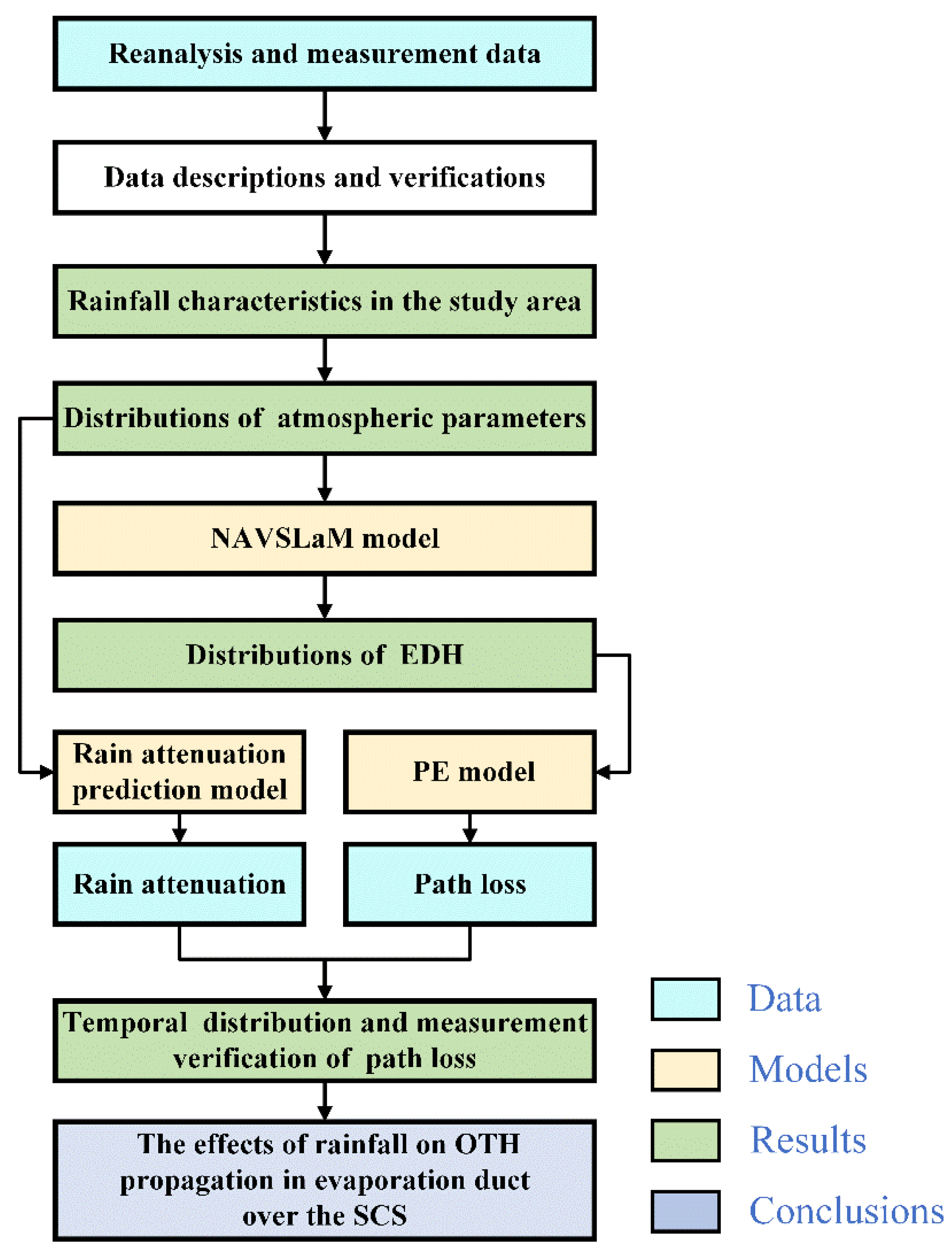
A research flowchart of this study is shown in Figure 1. The study area, methods and datasets are introduced in this section. In Section 3.1, the characteristics of annual rainfall in the study area and the distribution of rainfall density during the study period are introduced. In Section 3.2, the temporal and spatial distributions of several meteorological parameters are summarized, including rain rate (RR), WS, AT, SST, RH and air–sea temperature difference (ASTD). The distribution of the EDH and the sensitivity of the EDH to meteorological parameters are analyzed in Section 3.3. The simulated RA and PL are given in Section 3.4. The PL temporal distribution and measurement verification are also given in this section. The additional three experiment results and the effects of RR and total rainfall on OTH propagation are discussed in Section 4. The conclusions are given in Section 5.
2. Materials and Methods
2.1. Study Area
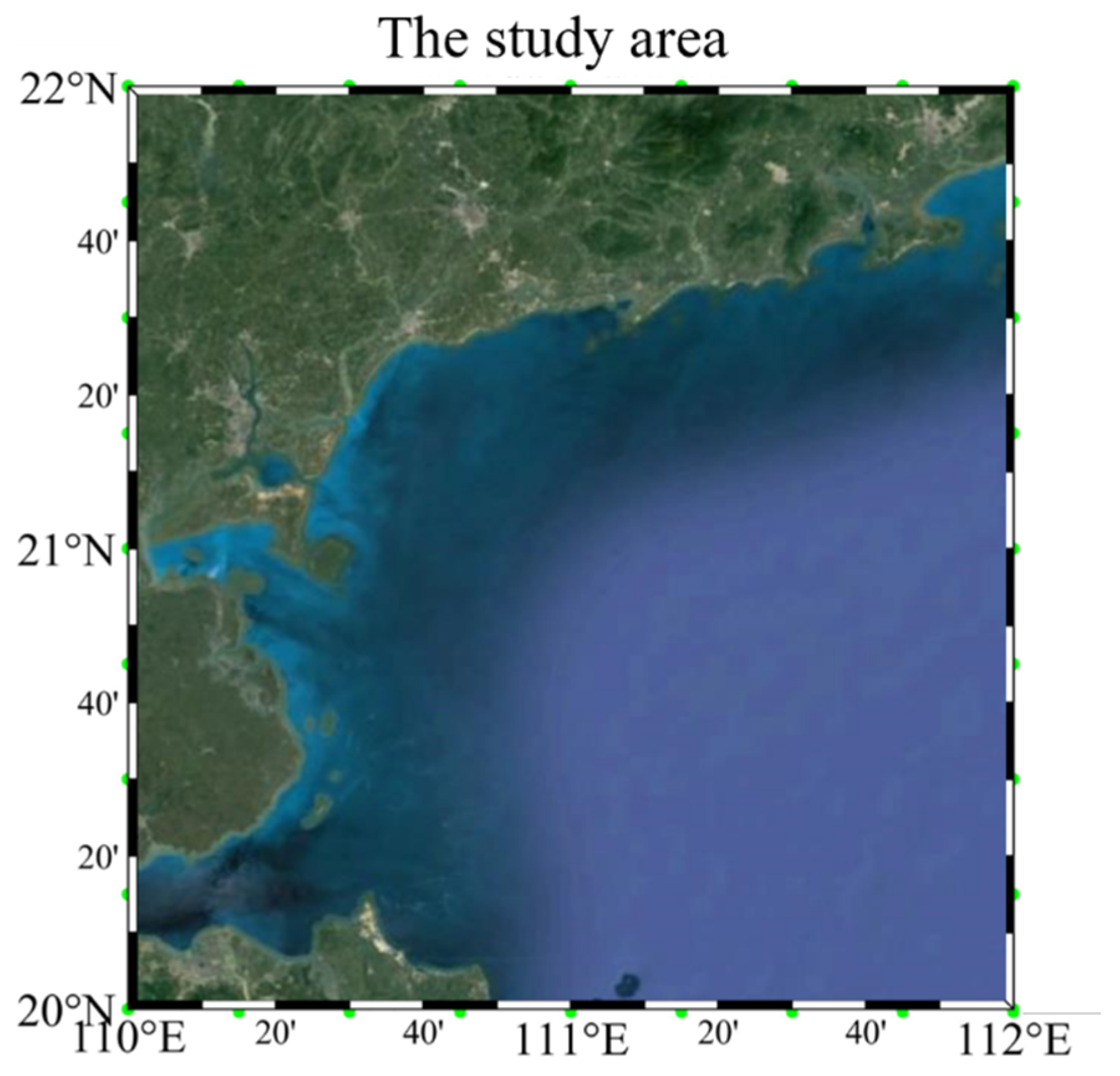
The SCS is one of the busiest international sea lanes. The tankers and merchant ships sailing through the SCS account for more than half of the world’s maritime transportation. The SCS is a marginal sea that is a part of the Pacific Ocean and encompasses an area from Singapore and the Malacca Straits to the Strait of Taiwan, comprising around 3.5 × 10⁶ km2. The climate of the SCS is significantly complicated [46].
To understand the effects of rainfall over a wide range of sea areas and obtain PL data during rainfall conveniently, the SCS (20°–22°N, 110°–112°E) was selected as the study area (Figure 2). The climate in this area is significantly influenced by the interaction of land and sea, causing abundant rainfall.
2.2. Datasets
2.2.1. Reanalysis Data
The meteorological data used in this study is the European Centre for Medium-Range Weather Forecasts (ECMWF) reanalysis version 5 (ERA5) single-level hourly data [47] from 1979 to the present, downloaded from the ECMWF database. The time resolution of ERA5 is 1 h, and the spatial resolution is 0.25° × 0.25°. Table 1 shows the sources, collection heights, units and abbreviations of the various types of data. The convective RR data are used in this study because this parameter is the rate of rainfall (rainfall intensity). In this study, RR and convective RR are considered equivalent. Moreover, the raindrops that fall on the sea surface are more convincing, as the ED is a phenomenon that occurs at the sea surface.
Before using the ERA5 reanalysis data, the credibility of the data is verified. Marine meteorological buoy data are not affected by land and survey ships and can be used to verify the credibility of the reanalysis data [48]. As long-term buoy observation data in the South China Sea (SCS) are difficult to obtain, the hydrometeorological data collected by the Tropical Atmosphere Ocean Buoy (TAO52087) are used in this section to verify the ERA5 reanalysis data. Details of the buoys, instruments and stations are provided by Meindl and Hamilton [49] and McPhaden et al. [50]. It is worth noting that the sampling height of the buoy data may be different from the reanalysis data, which is the main reason for the data discrepancy.
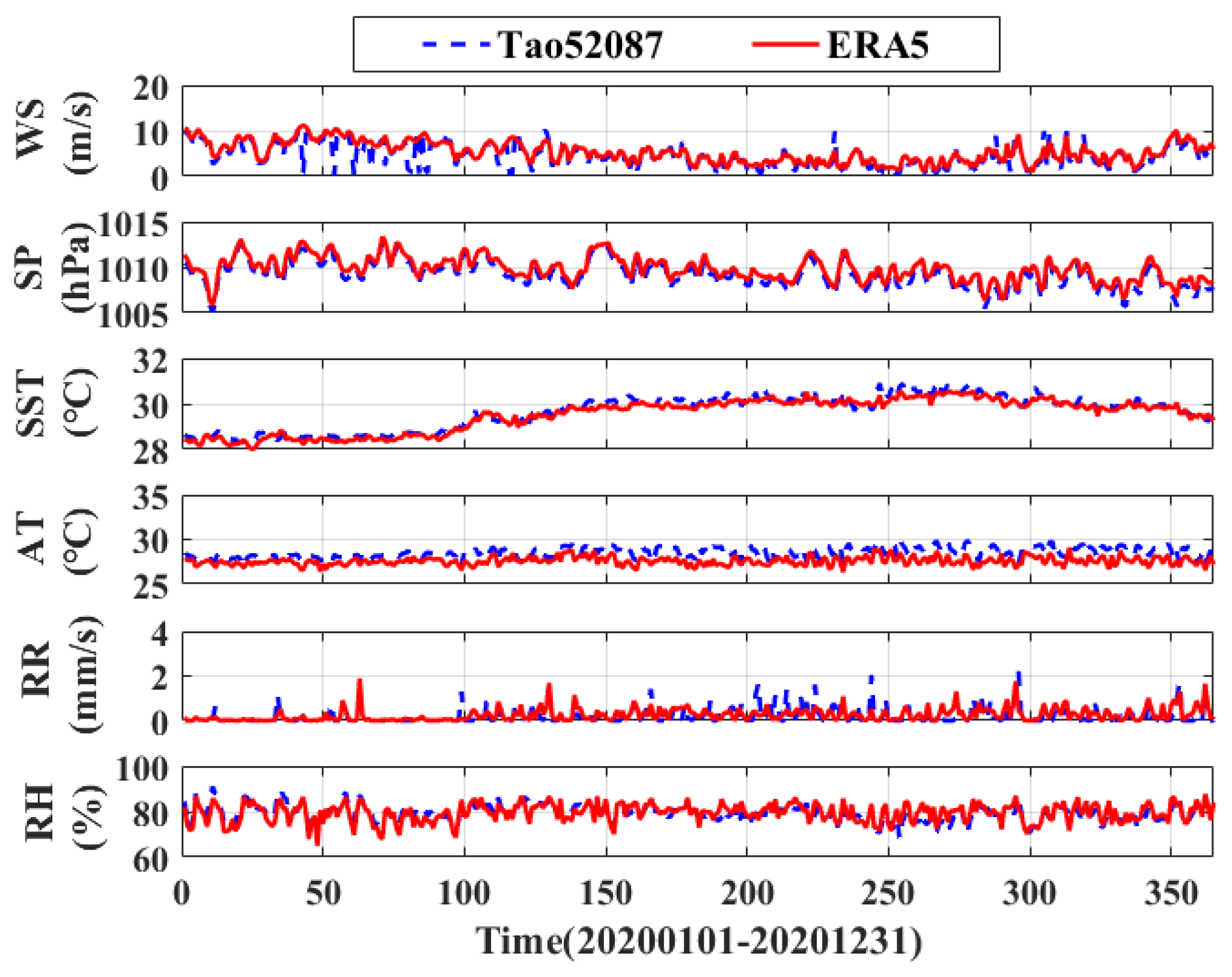
Owing to missing buoy data after March 2021, ocean and atmosphere data from the ERA5 hourly reanalysis data and the buoy data in 2020 are used for comparison (Figure 3). As the resolution of the buoy data is daily, the ERA5 reanalysis data are the average over 24 h. It can be seen from Figure 3 that the WS in the buoy data is abnormally low for a period of time during the initial time in 2020, which may have been caused by the movement of the buoy body caused by wind and waves. In addition, the results from the two datasets are relatively consistent.
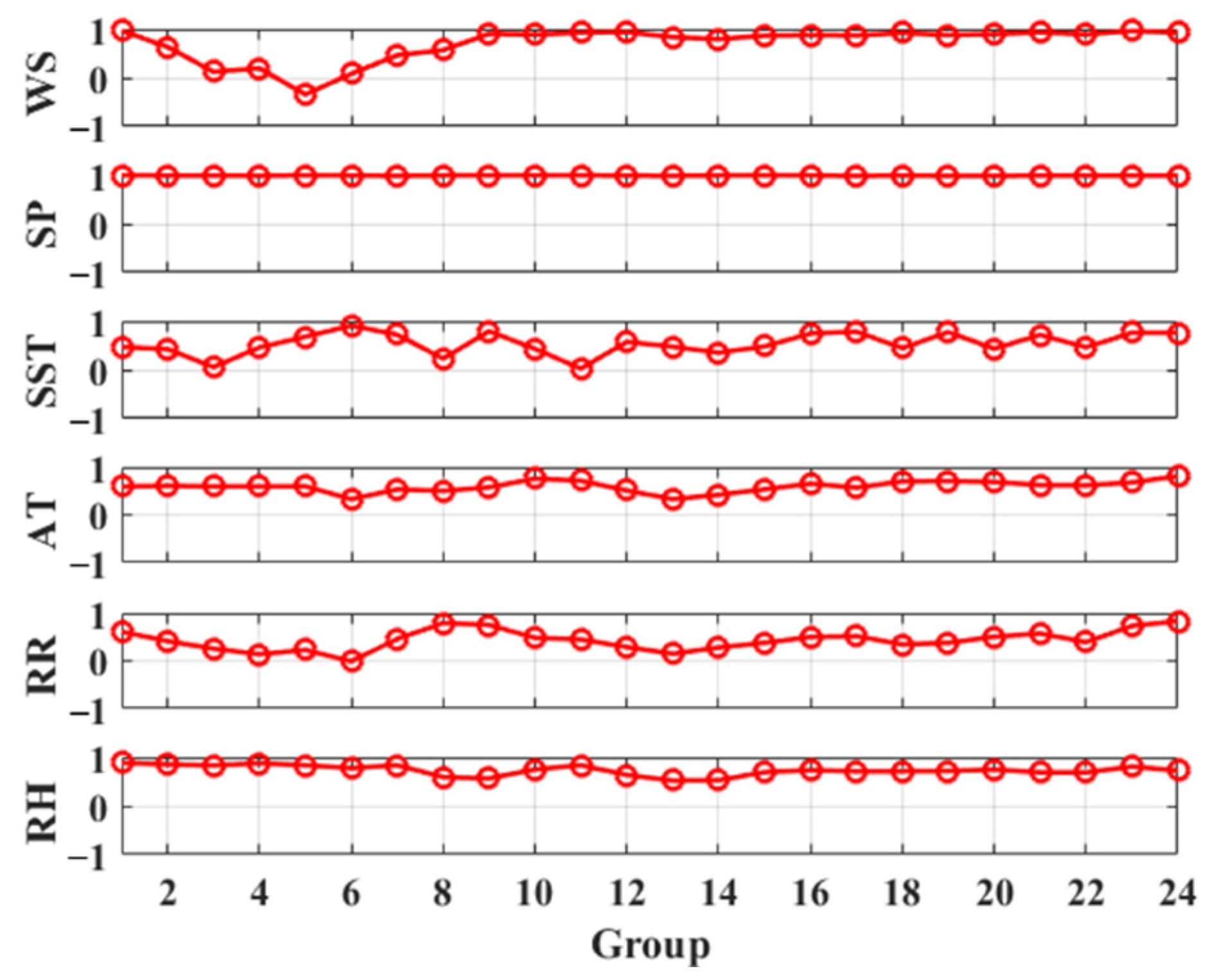
There are many ways to analyze the correlation of two time series [51,52]; the Pearson method is chosen in this article. Figure 4 shows the Pearson correlation coefficients of the two data sources, which is divided into 24 groups for analysis. There are 366 samples totally, and every 16 samples are formed in one group. The last group with insufficient data is supplemented by the samples of the previous group. It can be seen that the correlation coefficients of WS, SST and RR are close to 0 in the first eight groups, which might be caused by the different sampling heights of the TAO52087 and the ERA5 data. The average Pearson correlation coefficients of the WS, SP, SST, AT, RR and RH are 0.78, 0.99, 0.97, 0.61, 0.47 and 0.70, respectively. Two datasets show strong correlation in WS, SP, SST, AT and RH and moderate correlation in RR.
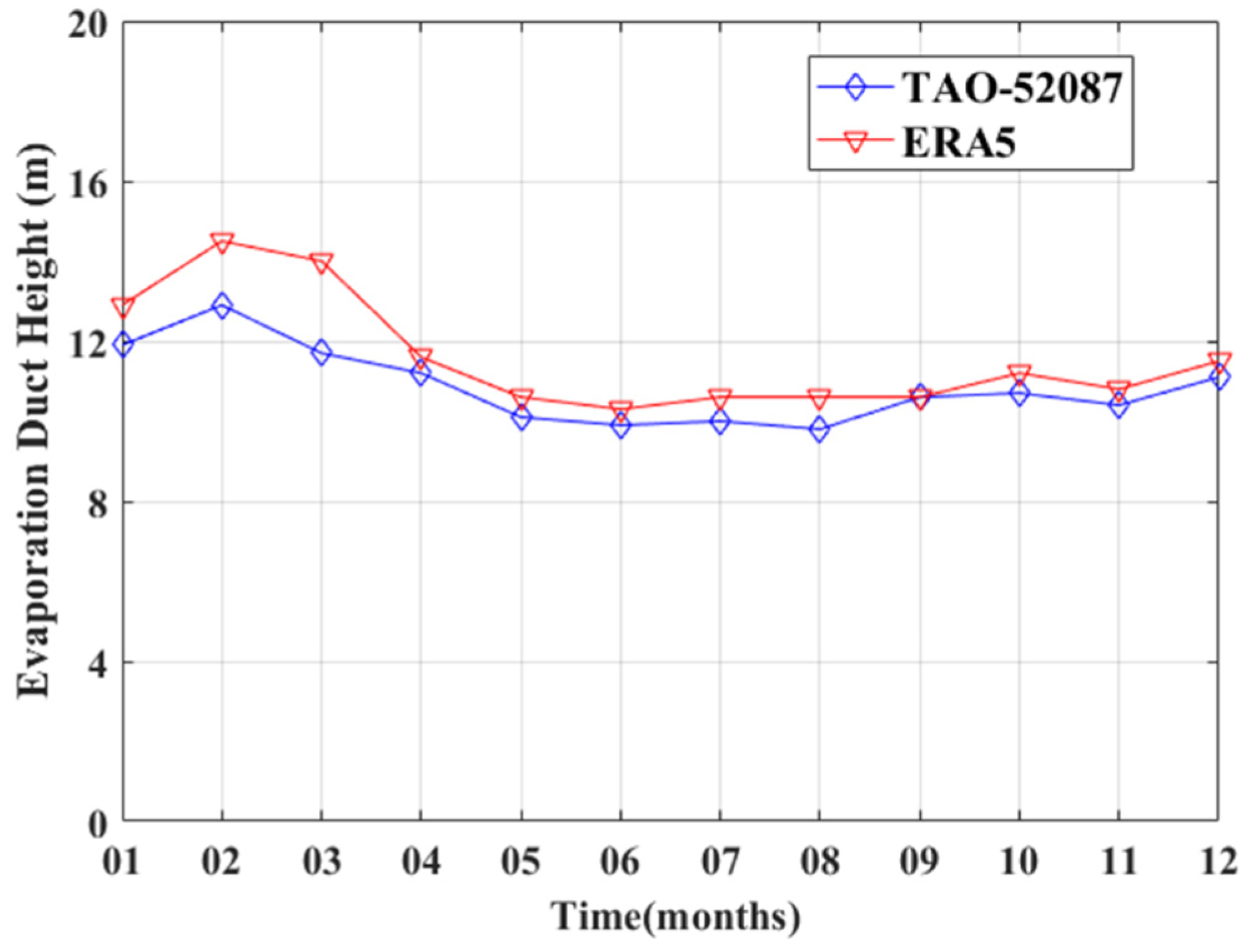
Furthermore, the monthly averaged values of the EDH calculated by the ERA5 reanalysis data and the TAO52087 buoy data are compared in Figure 5. It can be seen that the EDH calculated by the two data sources still maintains a relatively consistent variation trend. The maximum difference in the EDH between the ERA5 reanalysis data and the TAO52087 buoy data is 2.3 m, and the average difference is 0.74 m. The main reason for the differences in the EDH is the difference in the AT and the RH between the two data sources, which may be caused by the sampling heights.
2.2.2. Measurement Data
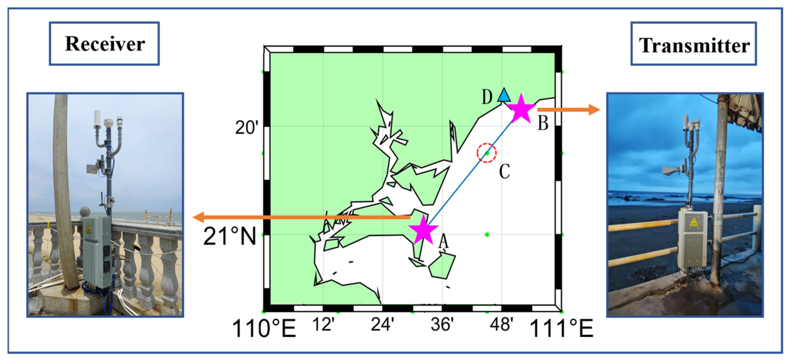
In 2021, an EM-wave propagation experiment was conducted in the northern area of the SCS. The experiment started at 18:00 on 21 November 2021 and ended at 16:00 on 22 November 2021 (UTC+8), which was selected as the study period. As shown in Figure 6, the transmitter was located at Jizhao Bay (point B) in Zhanjiang City, Guangdong Province, China. The receiver was located on Donghai Island (point A) in Zhanjiang City, Guangdong Province, China. The EM-wave propagation path was 53 km. Point C is the position of the ERA5 data grid point that the link passed. The grid points of hourly reanalysis data are from the ERA5 dataset in 2021 with a spatial resolution of 0.25° × 0.25°. Point D is the location of the Wuchuan Weather Station (WWS). The hourly meteorological data recorded by WWS were uploaded to the National Meteorological Information Centre of China Meteorological Administration (NMIC-CMA) where they can be downloaded by users. The data sources and the coordinates of points A, B, C and D are shown in Table 2.
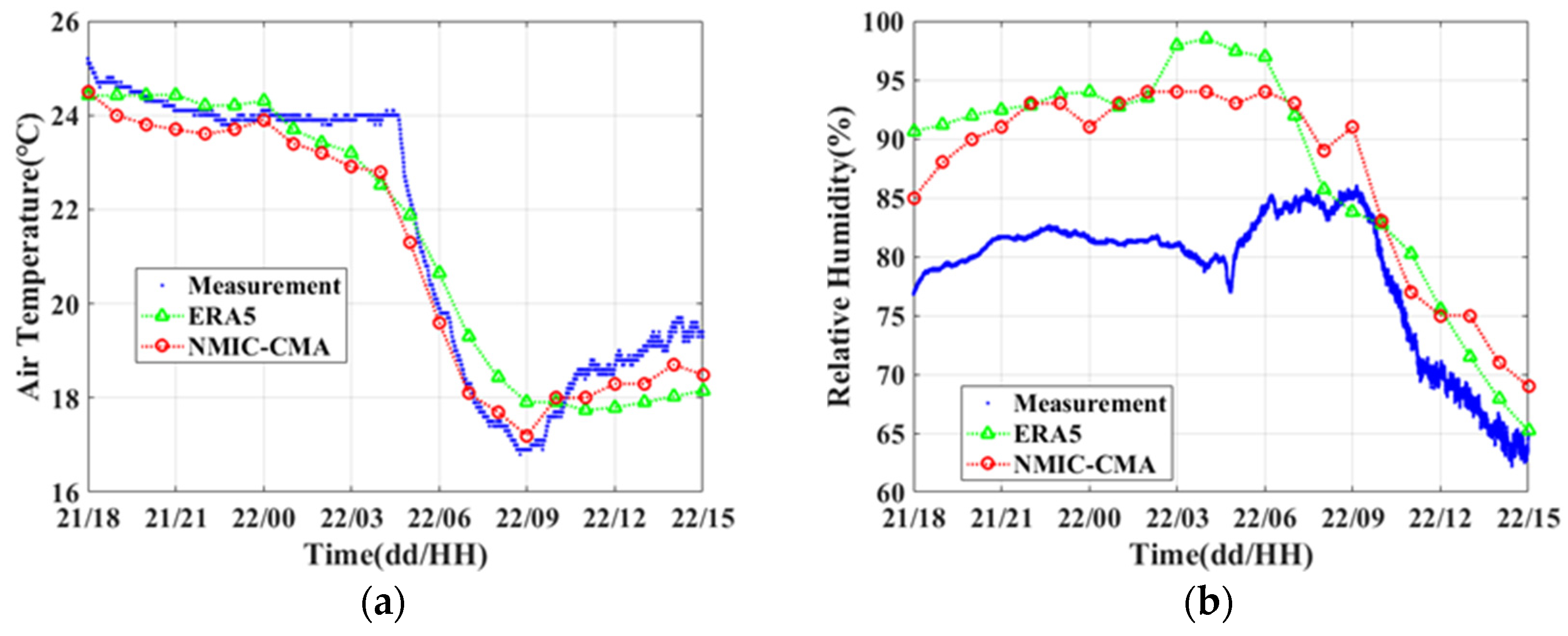
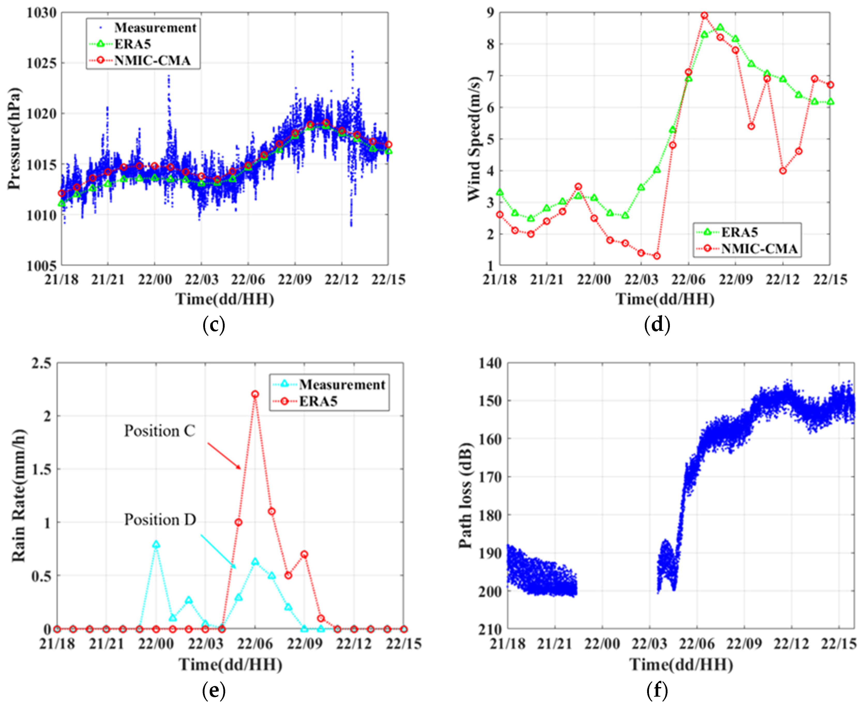
A comparison of the data from the experiment (position B, measured by the automatic weather station and the spectrum analyzer), the ERA (position C) and the NMIC-CMA (position D) during the study period is shown in Figure 7. The AT and the pressure from the three data sources show good consistency. The measured RH data in Figure 7b show a slight deviation at the start, possibly due to the location of sea–land border and the presence of buildings. The RR and WS data were not tested at point A and point B. Through the comparison of the ERA5 and NMIC-CMA data in Figure 7b,d, it can be seen that the distributions of the RR and WS have great regional differences. Owing to the system used in November, it was only possible to measure PL below 202 dB, and there were no signals between 22:22 on 21 November and 03:45 on 22 November. It can be concluded from Figure 7 that the ERA5 and NMIC-CMA datasets are usable for the OTH propagation link.
2.3. Methods
2.3.1. ED Prediction Models
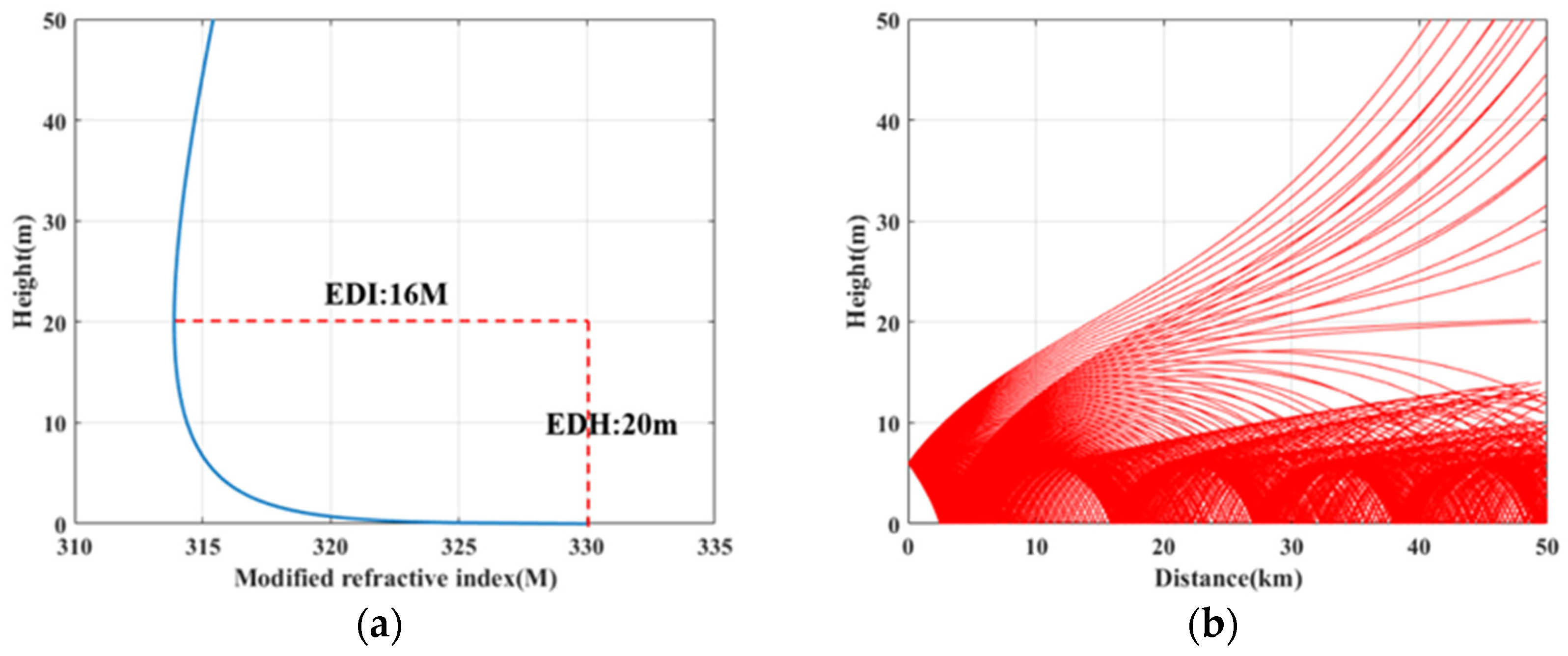
The ED is an atmospheric phenomenon that occurs near the sea surface owing to seawater evaporation. The ED profile can be directly obtained from the changes in the atmospheric modified refractive index in the vertical gradient. A typical ED profile is shown in Figure 8a. The height that corresponds to the lowest modified refractive index value in the overall profile is called the EDH. The difference between the modified refractive index profile at the height of the ED and at the sea surface is called the evaporation duct intensity (EDI). The EM-wave propagation trajectory of the ED profile in Figure 8a is shown in Figure 8b, where the trapping process of the EM waves can be seen clearly.
Methods to obtain the ED profile include direct measurement, model estimation and inversion. The direct-measurement method uses numerous meteorological sensors placed at different vertical heights to obtain the ED profile, which is not suitable for analyzing the statistical laws of the ED for large areas and long periods. In addition, the sea-clutter-inversion method needs high-power radar and higher antenna height, which means that EDs with a lower height may be missed. According to the global distribution of EDs, the average EDH is about 11 m above the sea surface near the Equator and at latitudes of less than 20° and decreases as the latitude increases [2]. In contrast, although there are some errors when compared with the measured values [1,5,53,54], the model estimation method is the most suitable method for ED study, especially for the study of the statistical laws.
Due to the better performance of the improved NAVSLaM among the several ED prediction models, it is used in this study to simulate the EDH and the ED profile. The equations of NAVSLaM were already proposed in References [5,9,55], and two necessary equations used in the calculations are as follows.
where T represents the air temperature, e is the water vapor pressure, z is a given height above the sea surface, p is the air pressure, N is the refractive index, and M is the modified refractive index.
2.3.2. The PE Model
The propagation of EM waves in free space is relatively simple and can be solved quickly by analytical methods. However, in practical applications, the propagation environment of EM waves is often complicated. The EM waves can be reflected, refracted and scattered repeatedly in irregular terrain, non-uniform atmospheric structure and rough sea surface conditions. The propagation becomes extremely complex, and it is difficult to obtain signals by analytical methods. Furthermore, the direct-measurement method cannot obtain effective data for every area and every step of EM-wave propagation.
Semi-empirical models combine a deterministic model with a specific propagation environment and attach a correction factor at the same time to explain the EM-wave propagation process in a complex environment. The calculation method is simple, and the running speed is relatively fast. For example, the commonly used PE model can solve the problem of EM-wave propagation in complex environments, such as complex terrain, rough sea surface conditions and horizontally inhomogeneous ED. Therefore, this study uses the PE model to study the propagation path of regional EM waves during rainfall.
The EM-wave PE has been gradually developed since the 1940s [22]. The step-by-step Fourier algorithm is the essence of the EM-wave PE, which transforms hyperbolic partial differential equations into parabolic partial differential equations through gradual dimensionality reduction [56]. Following this, scientists such as Dockery [57], Kuttler [58], Janaswamy [59] and Akbarpou [60] carried out in-depth research on the step-by-step Fourier solution of the PE, and a more stable PE system was developed with higher calculation accuracy. In 2004, Isaakidis [61] studied the finite-element method for the PE. Following this, [62] and Apaydi [63] also carried out related research on this basis and achieved satisfactory results.
In these previous studies, the Fourier transform is defined as:
where p is the angle relative to the horizontal direction, k is the wave number, represents the angle of propagation, and u is a scalar component given by:
where is the electric or the magnetic field.
Once the solution at is known as , the solution in distance can be calculated as [64]:
where and are the Fourier transform and the Fourier inverse transform, respectively.
The Parabolic Equation Toolbox version 2.0 (PETOOL v2.0, Ozlem Ozgun, 1 January 2020, Ankara, Turkey) [28] derived from the PE model is used in this study. PETOOL is a MATLAB-based one-way and two-way split-step PE software tool with a user-friendly graphical user interface for the analysis and visualization of radio-wave propagation over variable terrain and through homogeneous and inhomogeneous atmosphere. PETOOL was updated in 2020. Several ED models and a three-dimensional coverage map for the propagation factor and loss on real terrain data have been developed in this new toolbox.
2.3.3. RA Prediction Model of EM Waves
When EM waves propagate in the atmosphere, they are affected by absorption, attenuation, scattering effect, polarization and trapping effect due to the influence of atmospheric media, such as rainfall. The current RA prediction models all need to solve the attenuation characteristics, which are related to the spectral distribution and polarization mode of the rainfall. De Wolf [65] found that even with the same RR, the size of the raindrops varies widely. In view of the difficulty in obtaining the spectral distribution and polarization mode of rainfall, the RA prediction model recommended by the International Telecommunication Union (ITU) is used to describe the attenuation effect of rainfall in the rest of this article. Several studies [35] of the RA prediction model have shown that when the rainfall intensity is lower than 5 mm h−1, the differences between the ITU model and various RA prediction models are small.
According to the attenuation-specific model used on rainy days recommended by ITU, the attenuation owing to rainfall should be calculated from knowledge of RR. The specific attenuation (dB km−1) was obtained from the RR (mm h−1) using the power–law relationship [66]:
Values for the coefficients k and α were determined as functions of the frequency, f (GHz), in the range from 1 GHz to 1000 GHz, from the following equations, which have been developed from curve fitting to power–law coefficients derived from scattering calculations:
where f indicates frequency (GHz), k indicates kH or kV, α indicates αH or αV, H stands for the horizontal polarization, V stands for vertical polarization, and aj, bj, cj, mk and ck are constants.
3. Results
3.1. Rainfall Characteristics
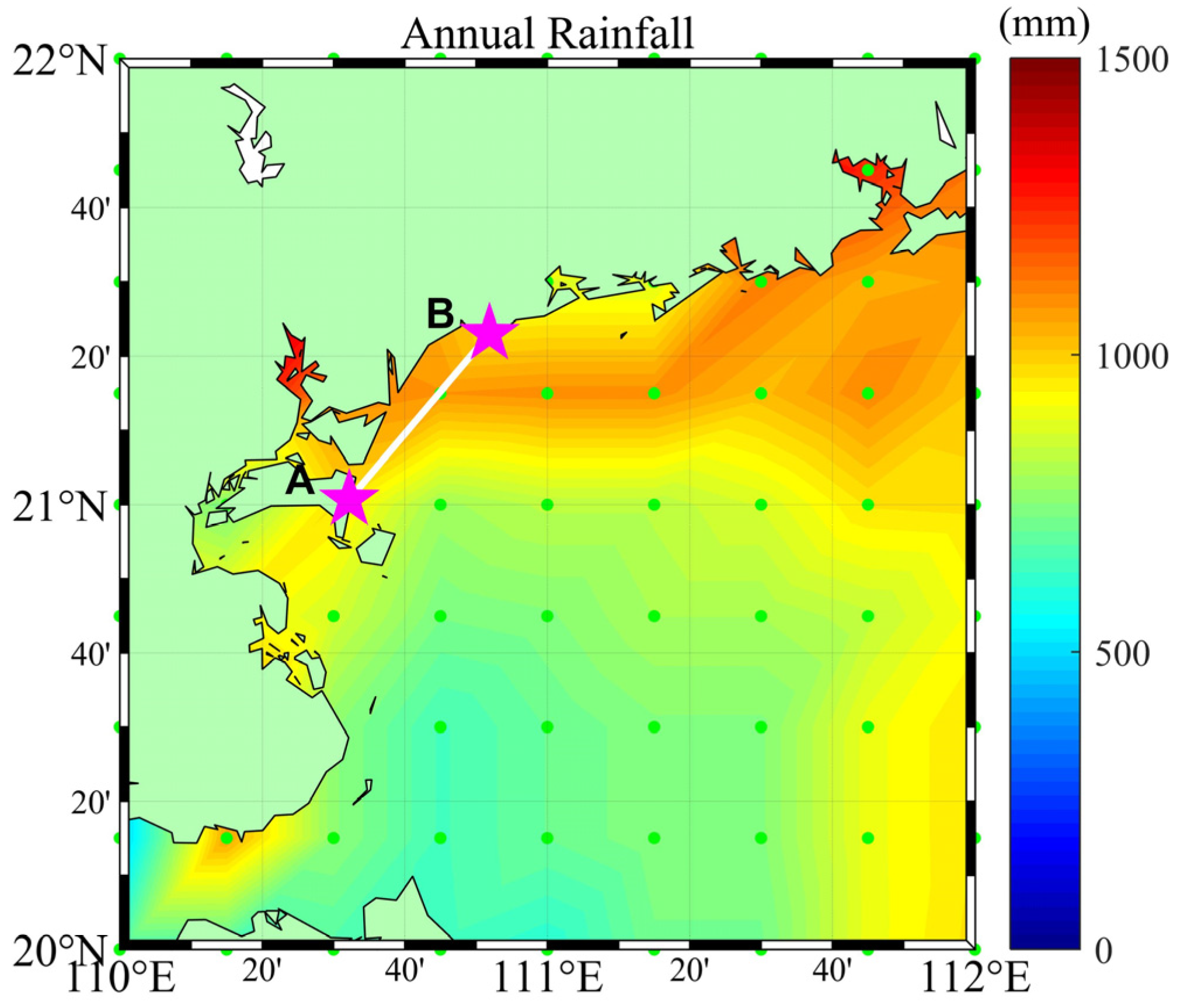
The annual RR in 2021 in the study area is shown in Figure 9. Owing to monsoons [67] and typhoons [68], the RR was relatively high in the study area and the annual rainfall was more than 500 mm in the most areas. The monsoon from the ocean is more likely to result in rain at the coast. In particular, at latitudes above 21°N, the annual rainfall reached up to 1500 mm. Rainfall causes changes in the atmospheric environment and ocean parameters such as AT, SST, RH and WS [69,70].
The study period from 18:00 on 21 November 2021 to 16:00 on 22 November 2021 (UTC+8) was divided into three parts, including the period before, during and after the rainfall. The rainfall lasted for a total of 9 h, causing changes in WS, AT, SST, RH, ASTD, EDH and PL, according to the records. At the beginning, the rainfall density reached the maximum of 0.79 mm s−1 at 0:00 on 22 November 2021. Then, the rainfall density decreased to 0.01 mm s−1 at 4:00 on 22 November 2021. After that, the rainfall density increased to 0.63 mm s−1 at 6:00 on 22 November 2021 and began to decrease till disappeared after 8:00 on 22 November 2021.
3.2. Atmospheric Parameters
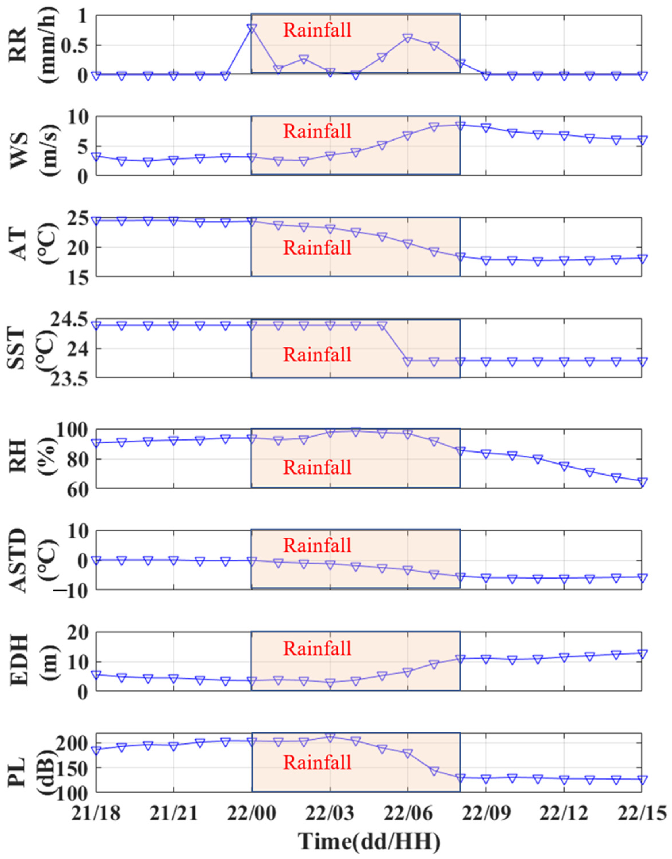
Figure 10 shows the evolution of the RR, WS, AT, SST, RH, ASTD, EDH and PL during the study period at position C. The rainfall period is indicated by a light pink box from 0:00 to 08:00 on 22 November 2021. The units of these parameters are the same as in Table 1. In general, the EDH is insensitive to the changes in SP [71], thus, the SP is not mentioned in the rest of this article.
Before the rainfall, the WS was lower than 3.4 m s−1, the AT was higher than 24.2 °C and the SST was steady at 24.38 °C. The RH was over 91% and had been increasing from 18:00 on 21 November. The ASTD decreased from 0.03 °C to −0.17 °C, which means that the atmospheric stability changed from stable conditions to unstable conditions.
During the rainfall, the RR decreased to nearly 0 mm s−1 at 04:00 and then increased to 0.6 mm h−1 at 06:00. The WS increased from 3.1 m s−1 to 8.5 m s−1. The AT decreased to 18.4 °C. The SST dropped by 0.59 °C between 05:00 and 06:00. The RH first increased to a maximum value of 98.53% at 04:00 and then began to decrease. The ASTD decreased to −5.4 °C.
After the rainfall, the WS remained at a high level and slowly decreased to 6.0 m s−1 at 16:00. The AT remained at a low level, around 18 °C. The SST remained steady at 23.79 °C. The RH dropped from 85.7% to 63.7%. The ASTD remained at a low level, around −5.8 °C.
For the whole study period, the WS increased after the rainfall compared with that before the rainfall. The RH had been close to saturation before the rainfall. The RH, AT, SST and ASTD decreased after rainfall compared with that before rainfall. Unlike over land, there is no evidence for a decreasing precipitation event duration with increasing SST [72]. As the specific volume of seawater is higher than that of the air, changes in the SST are slighter and slower than the changes in the AT when rainfall occurs. Furthermore, the correlation between evaporation and the ASTD is much stronger than that with SST [73]. Hence, the AT and SST are combined into ASTD in the rest of this article.
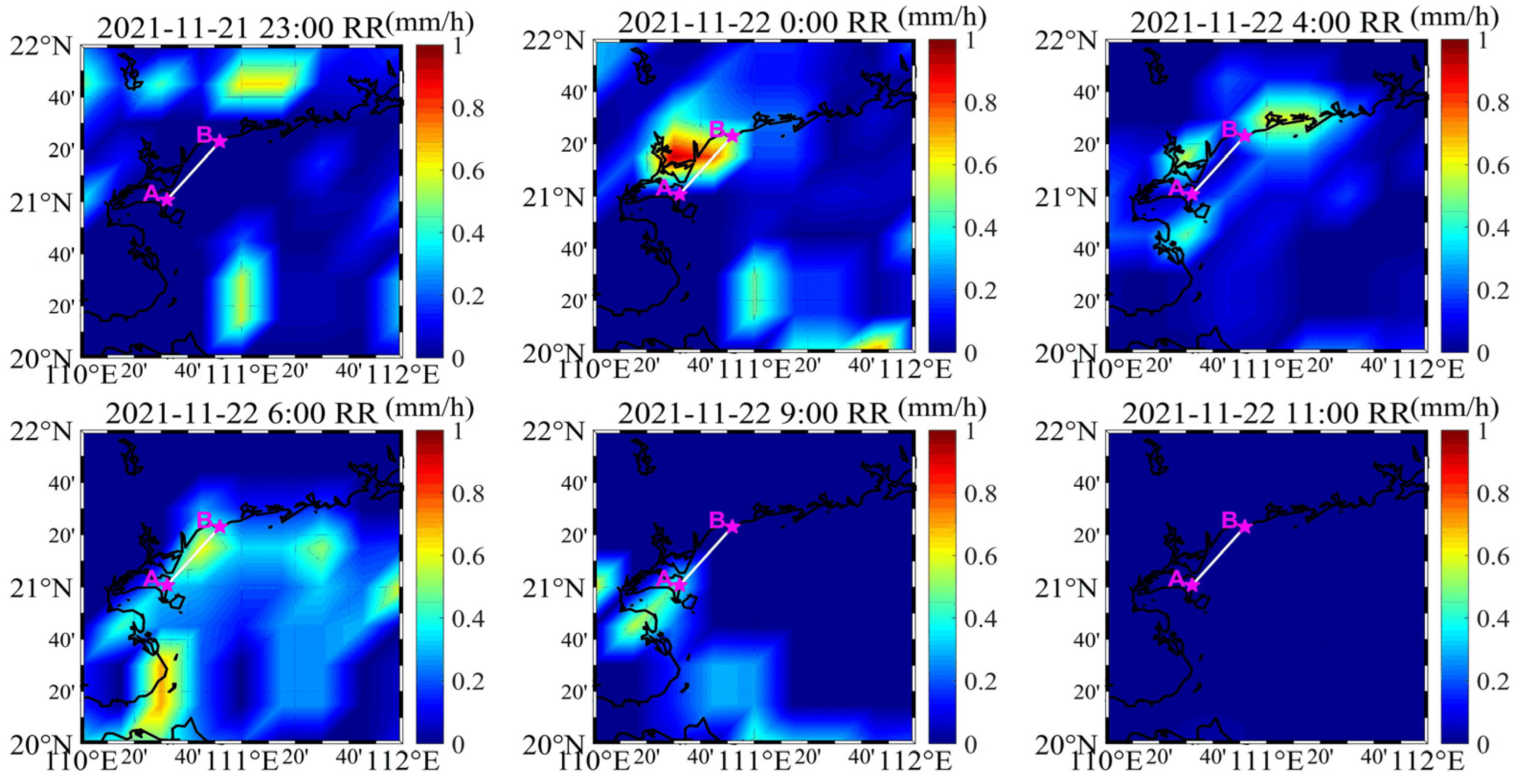
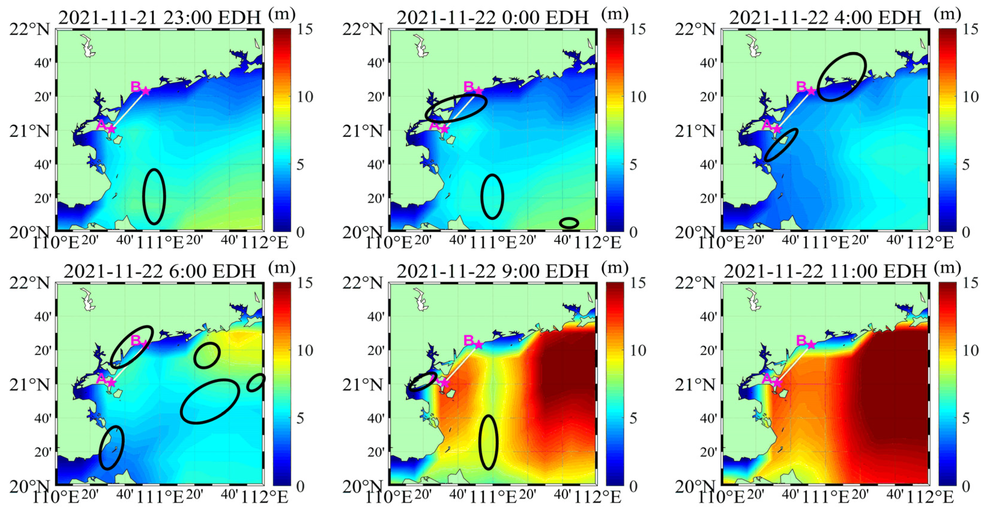
Rainfall often occurs over a large area, and the meteorological changes at a single location cannot accurately reflect the effects of rainfall. In addition, the ED distribution over a large area of the sea is also needed for the OTH propagation link. Therefore, six typical time points (23:00 on 21 November, and 00:00, 04:00, 06:00, 09:00 and 11:00 on 22 November) were selected to analyze the evolution of the regional meteorological parameters. The data were downloaded from the ERA5.
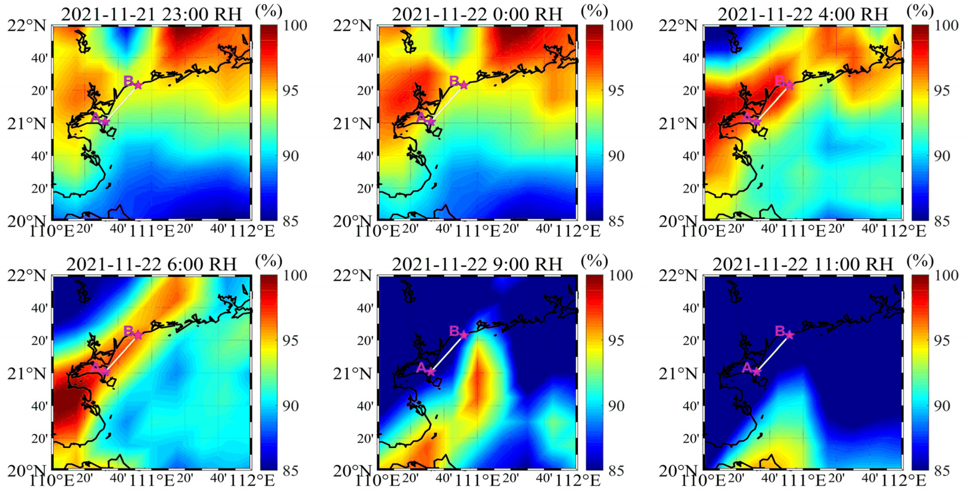
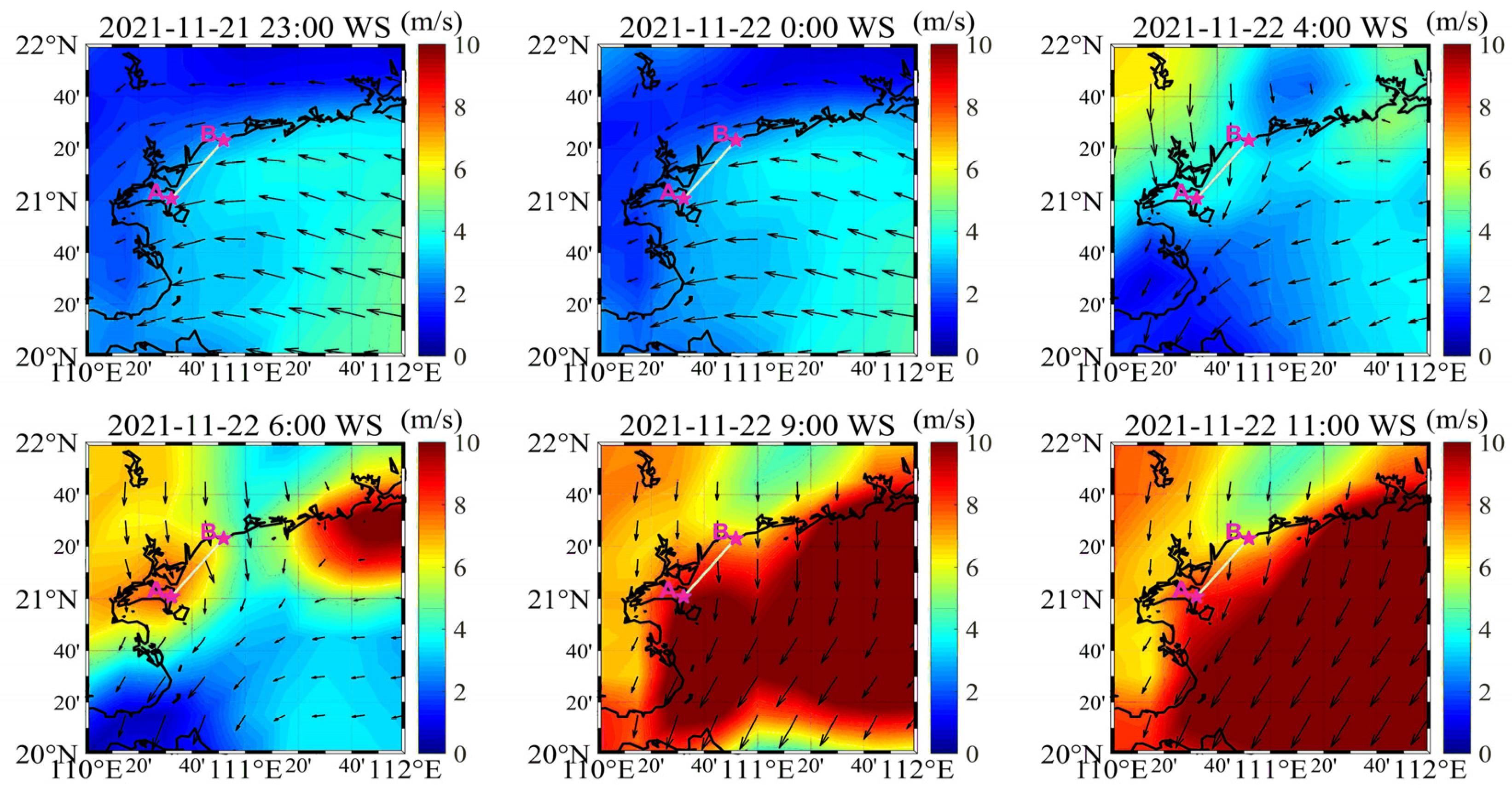
Figure 11 shows the spatial distribution of RR in the study area at the six times. The rainfall area almost covered the OTH propagation link between positions A and B at 00:00 and 06:00 on 22 November. There was a little rainfall around position B at 04:00 on 22 November and position A at 09:00 on 22 November. Figure 12 shows the spatial distribution of RH in the study area at the six times. The RH was relatively high around the coast before 06:00. The moist patches moved along the coastline from west to east at first, then moved towards the south. Figure 13 shows the spatial distribution of the WS and wind direction in the study area at the six times. The WS was less than 5 m s−1 at the start. Then, strong winds over 10 m s−1 appeared from the west coast and the east coast in the study area at 06:00 on 22 November and eventually met in the middle of the study area. The whole area was covered by strong winds after 9:00 on 22 November.
The wind came from the east and moved to the west, and the moisture from the evaporation of seawater was transported to the edge of the land by the wind, creating strong RH at the coast (Figure 12). From 04:00 on 22 November, the wind turned toward the south, and the moist patches were transported to the south at the same time (Figure 12).
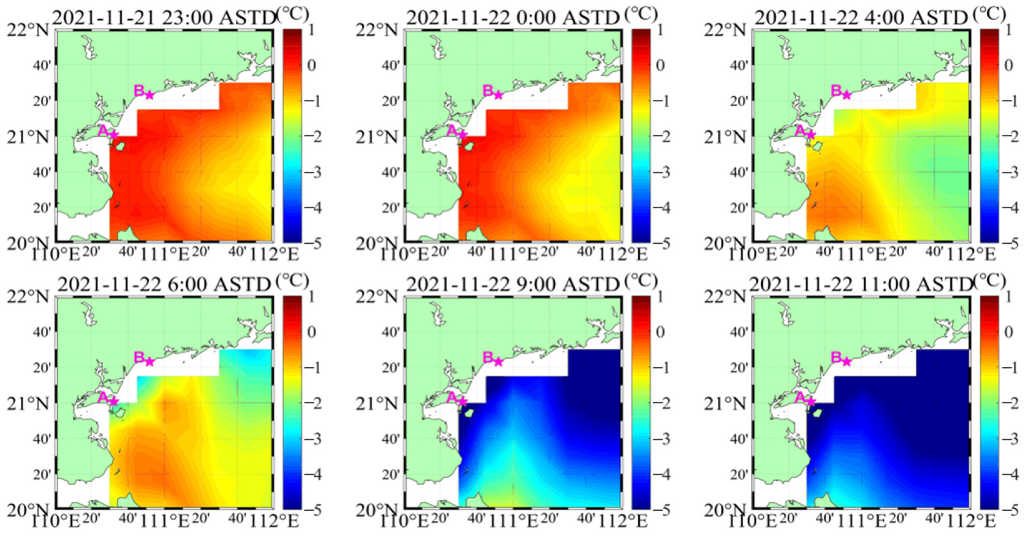
Figure 14 shows the spatial distribution of the ASTD in the study area at the six times. As shown in Figure 14, the ASTD was higher than zero before 04:00 on 22 November in the areas close to the coast and lower than zero after 04:00 on 22 November. The ASTD became increasingly lower in the study area, especially after 04:00 on 22 November. An interesting find is that the atmospheric conditions were more unstable where the WS was stronger and vice versa. When the ASTD close to land was considered as the difference of land air and sea surface, the changes in the ASTD caused a sea–land breeze that eventually affected the wind direction.
In summary, rainfall occurred with a series of atmospheric processes. Under the effects of the sea–land breeze, the wind direction and WS changed immediately. Strong WS and the change in wind direction caused the moist patches to move during the rainfall, which eventually affected the RH. The RH at position C was almost saturated before the rainfall and unexpectedly decreased during the rainfall. The WS after rainfall was higher than that before rainfall and changed its direction during rainfall. The ASTD values changed from positive to negative near the coast under the effects of rainfall.
3.3. EDH Analysis
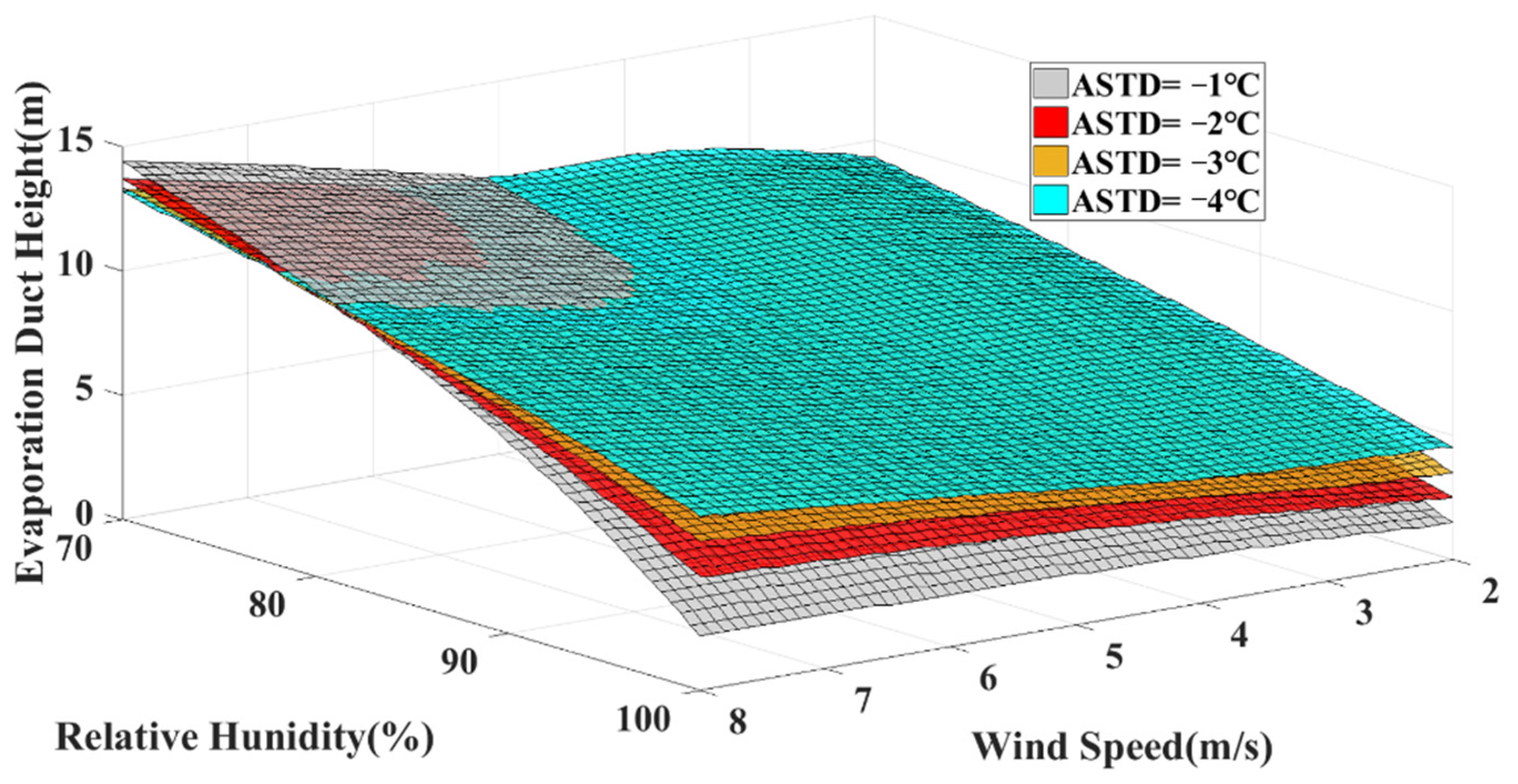
The NAVSLaM was used to study the sensitivity of the EDH to the ASTD, WS and RH (Figure 15). The SST was 24 °C and the pressure was 1015 hPa, which are the average values in the study area. As seen in Figure 15, a high EDH is usually accompanied by low RH and strong WS. Using the data in Figure 15, the ranges of the EDH under different ASTD values are shown in Table 3. The gradient of the EDH decreased with decreasing ASTD. When the RH was over 85% or the WS was under 5 m s−1, the decrease in ASTD accelerated the changes in the EDH. Therefore, the increasing WS accompanied with the decreasing RH led to an increase of the EDH during rainfall; the growth rate of the EDH was inversely proportional to the value of the ASTD under this condition.
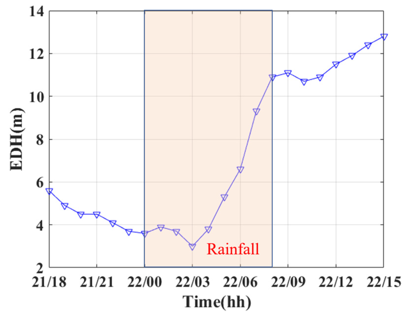
Figure 16 shows the evolution of the EDH during the study period at position C. The rainfall period is indicated by the light pink box from 00:00 to 08:00 on 22 November.
Before the rainfall, the EDH was at a low value and decreased in this period. The wind had already brought some moist patches into the area, leading to a high RH value.
During the rainfall, the EDH decreased before 03:00 on 22 November owing to the increasing RH. After that, the EDH increased for two reasons: the increasing WS and almost constant RH between 03:00 and 04:00 on 22 November and the decreasing RH accompanied by increasing WS after 04:00 on 22 November.
After the rainfall, the EDH continued to increase for a period of time. This is because the RH continued to decrease after the rainfall, and the WS was much higher than before the rainfall.
Figure 17 shows the spatial distribution of EDH in the study area at the six time points. In most ellipses, the EDH was significantly lower than that in the surrounding areas without rainfall. Moist patches can apparently affect the distribution of the EDH. In particular, at 09:00 on 22 November, the high RH caused a low-EDH region around 111°E during rainfall.
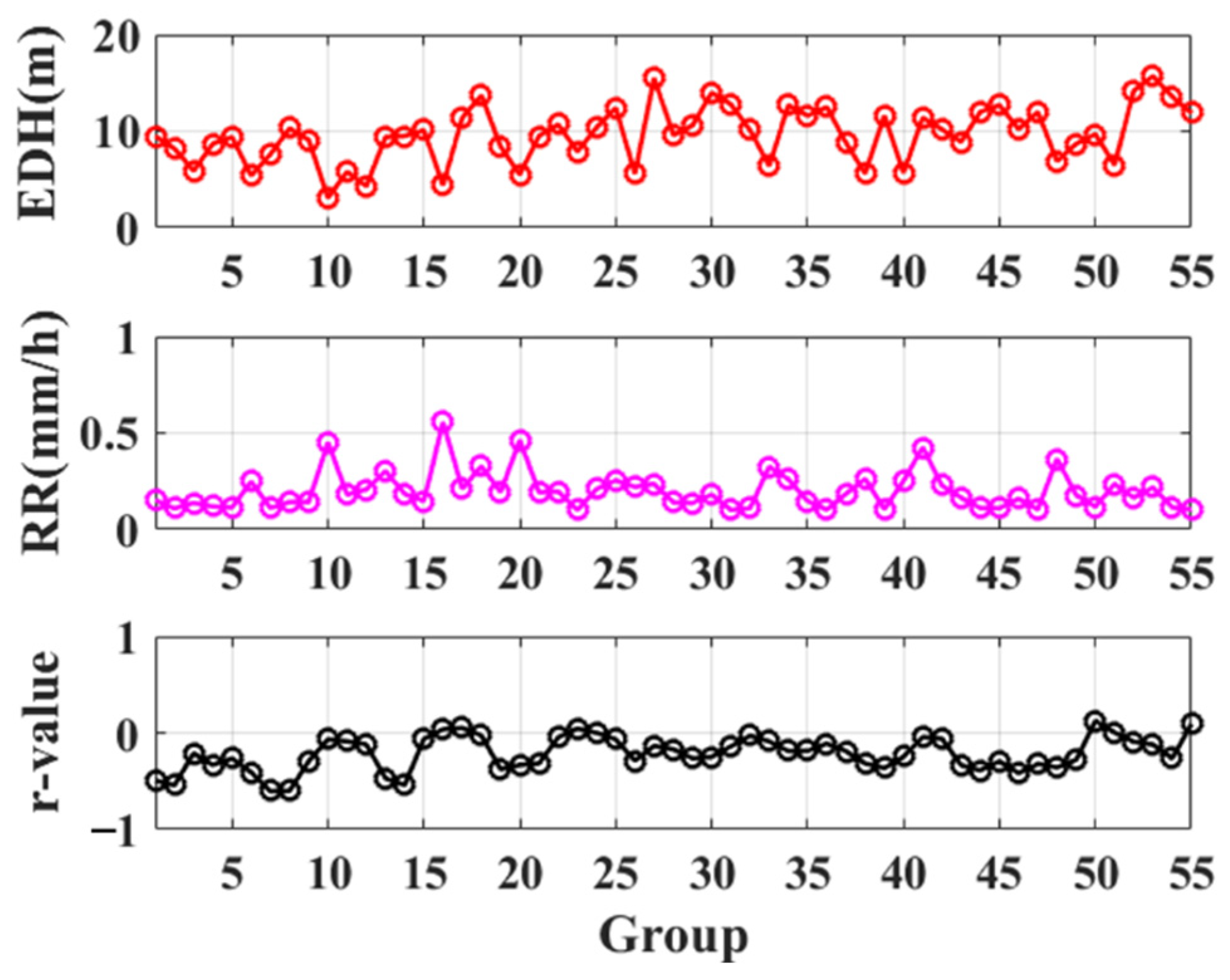
The Pearson correlation coefficients of the EDH and RR are shown in Figure 18. After removing the data on land and the data without rainfall, there were 833 samples. The preprocessed data was divided into 55 groups. Every 16 samples were formed in one group. The last group with insufficient data was supplemented by the samples of the previous group. It can be seen from Figure 18 that there is a negative correlation between RR and EDH. Most of the correlation coefficients are lower than 0. A small number of points close to 0 may be affected by other complex marine environments, such as the sea–land breeze. The average Pearson correlation coefficient of the EDH and RR is −0.18, which shows a weak negative correlation.
In summary, rainfall causes changes in the atmospheric environment and ocean parameters that eventually affect the EDH. In the study area, the EDH decreased during rainfall in most cases. In the study period, the EDH was low before and during rainfall owing to the high RH and low WS. However, the EDH increased during rainfall when the WS was becoming stronger, and the moist patches brought by rainfall were moved. The EDH remained higher after the rainfall owing to the lower RH.
3.4. PL Analysis
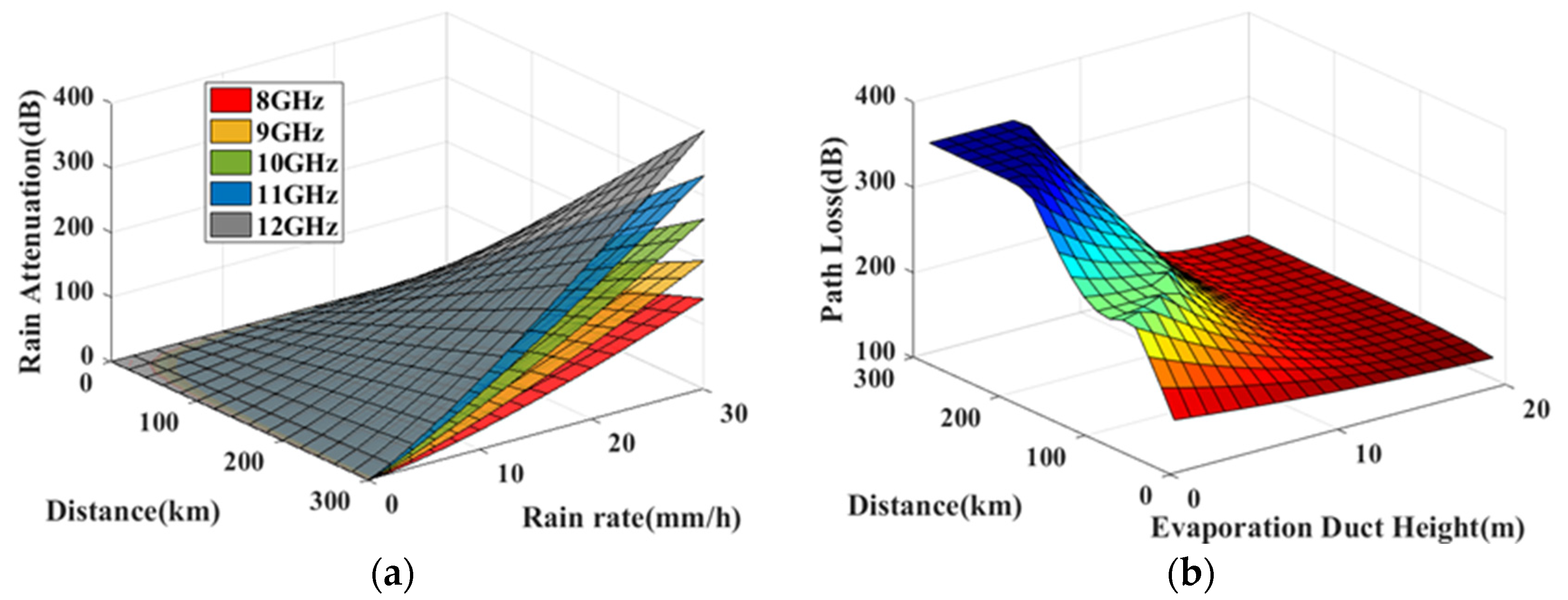
In this section, RA and PL are estimated by the ITU calculation model and the PE model, respectively. The simulation parameters used in the PE model are shown in Table 4. The effects of the ED and RA on the propagation of EM waves at sea is shown Figure 19.
As shown in Figure 19a, RA is a function of EM-wave frequency, distance through the rain region and rainfall intensity (equal to RR in an hour), according to the ITU model. It is evident that when the frequency is constant, RA generally increases with increasing distance and RR. When the frequency changes, a decrease in frequency leads to a marked decrease in RA. When RR is less than 5 mm h−1, the maximum attenuation of the EM waves in the range of 8–12 GHz caused by the rainfall is 0.16 dB km−1.
Using several samples of ED profiles generated by the NAVSLaM, the PL within 300 km in Figure 19b shows an origami-crane-like structure. The peak of the PL difference for the mean distance surpasses 0.69 dB km−1. When the EDH is less than 5 m and the distance is below 50 km, the PL is less than 180 dB. However, once the distance reaches 60 km with an EDH less than 5 m, the PL exceeds 200 dB. In contrast, when the EDH is more than 11 m, the PL of the EM-wave propagation to 300 km does not exceed 200 dB.
Furthermore, the effect of the ED on PL reaches 0.69 dB km−1 on average, which is 4.3 times stronger than the maximum RA (0.16 dB km−1), when the rainfall is less than 5 mm h−1. The propagation of EM waves over the sea is still mainly affected by the ED. Thus, the marine EM-wave systems should be suitable for using the optimal frequency band for the best ED during rainfall under 5 mm s−1.
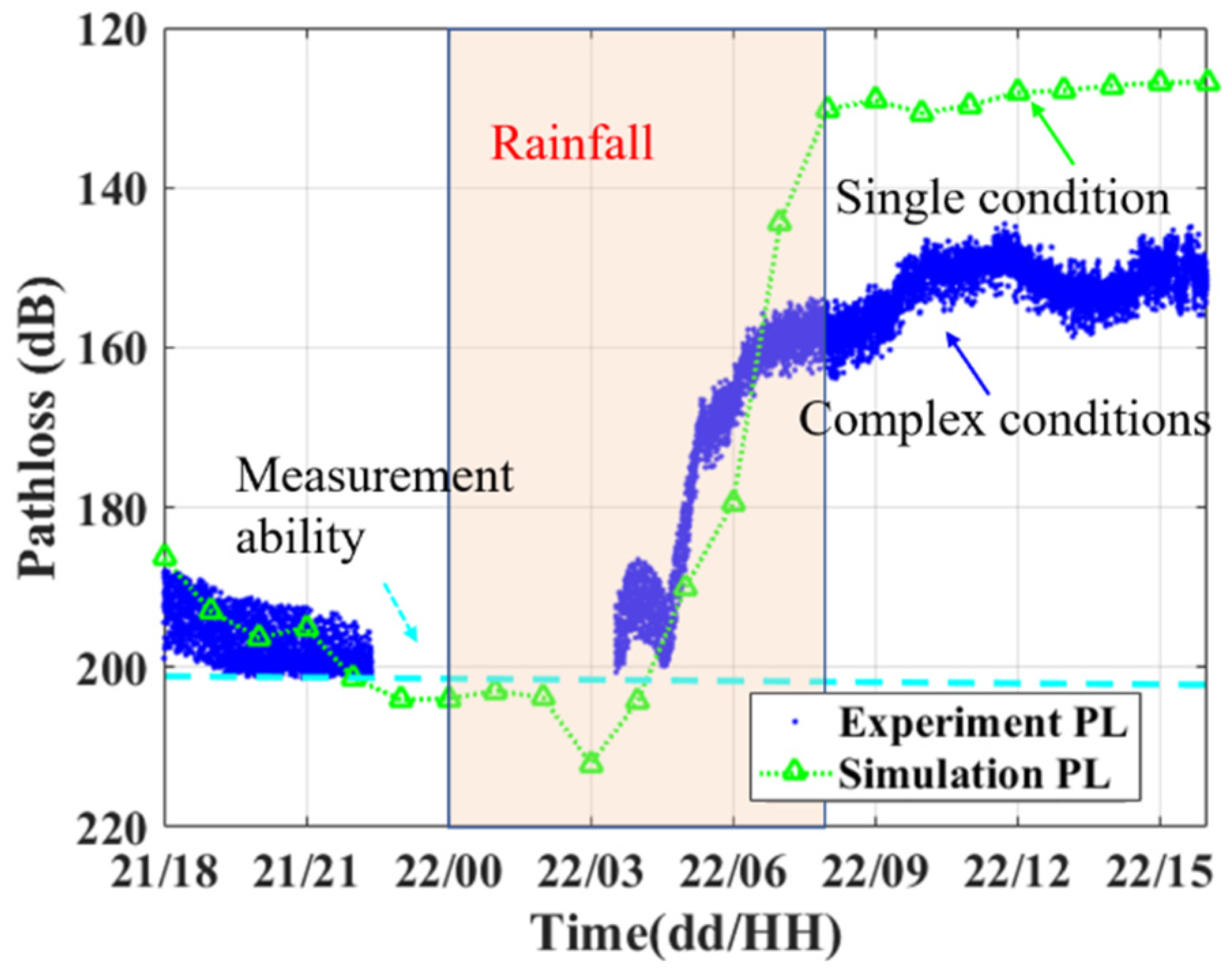
Figure 20 shows the simulation and measurement curves of the EM-wave PL in the ED during rainfall. The EM wave was transmitted from Jizhao Bay and was received at Donghai Island after propagating 53 km. The received signal level was recorded every four seconds by a computer. The experimental configurations are shown in Table 5. The frequency of the EM wave is 8.0005 GHz. Although the simulation PL included the RA during rainfall, the RA according to the ITU is less than 5 dB. In fact, the PL difference in Figure 20 is over 50 dB and rapidly changes within an hour.
It can be seen in Figure 20 that the simulated PL is strongly consistent with the measured PL, and their trends are similar. The simulated PL shows the opposite trend to the EDH (Figure 16). The simulated PL increased to a maximum value of 212.1 dB at 03:00 on 22 November. After that, the increase in the EDH resulted a decrease of the simulated PL, until the simulated PL decreased to 130.1 dB at 08:00 on 22 November during rainfall. The measured PL gradually decreased to 157.6 dB at 08:00 on 22 November and decreased slowly for a period of time after rainfall. The movement of moist patches caused by a sea–land breeze brought a 7.1 m increase of EDH and a 42.4 dB decrease of PL, which was an abnormal phenomenon during rainfall.
The difference between the measured PL and the simulation PL after 07:00 on 22 November was mainly produced by the OTH link, where only one grid point at the position C was used, rather than the range-dependent modified refractivity profiles along the OTH link. Moreover, complex conditions such as inhomogeneous ED, waves and surface roughness would affect the simulation PL.
In summary, the effect of RA on OTH propagation owing to rainfall is much less than the effect of the ED when the RR is under 5 mm s−1. The PL is at a high value before and during rainfall but decreases during rainfall when the WS increases and the RH decreases. Furthermore, the PL decreases after rainfall when the RH continues to decrease.
4. Discussion
Both the RR and total rainfall can produce a great influence on the meteorological factors over the sea. Therefore, this section discusses the effects of RR and total rainfall on OTH propagation and verifies the results in Section 3.
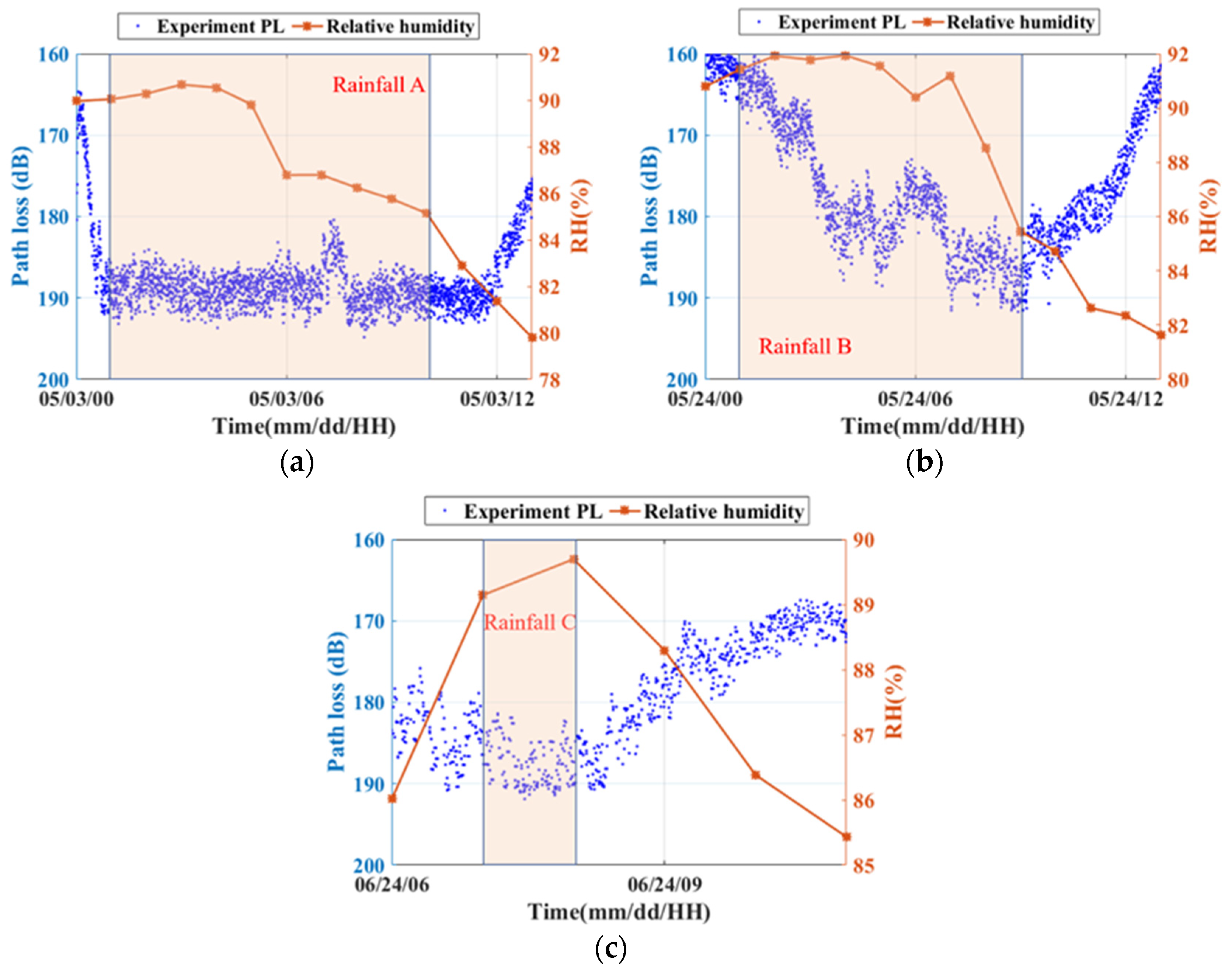
To further verify the conclusions, the three additional experiment results are given in Figure 21. The experiment was also held in the SCS in 2021 with different equipment of an omnidirectional antenna at the receiver. The three rainfall events are chronologically labeled as Rainfall A, Rainfall B and Rainfall C.
The rainfall brought the near-saturated humidity in Figure 21a and an increasing RH in Figure 21b, causing a higher PL. The lower RH after rainfall caused PL below 180 dB. However, these three observations did not show a decreasing PL during rainfall due to the absence of the direction change of the sea–land breeze. It is worth noting that the rainfall intensity during all three rainfall periods did not exceed 5 mm h−1, which means the EDH was still the main impact factor of the OTH propagation link, rather than the RA.
In summary, these three additional experiment results showed that the PL decreased to a lower value with the high humidity, which is consistent with the results of Section 3.
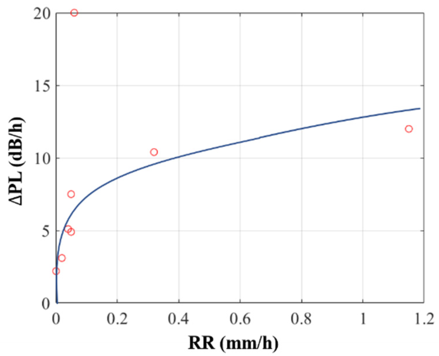
With the data of RR and PL from the additional experiment results, Figure 22 shows the relationship between RR and ∆PL. The ∆PL is the hourly increased value of PL and is calculated by:
where represents the hourly averaged PL, and represents the hourly averaged PL one hour before .
As Figure 22 shows, the fitting curve is a logarithmic function of ∆PL and RR. When the RR is over 0.5 mm h−1, the ∆PL exceeds 10 dB h−1. According to this trend, ∆PL will eventually increase to about 18 dB h−1 and no longer change with RR, which needs to be verified by more observations.
To discuss the effects of total rainfall on OTH propagation, the parameters of the additional experiment results during rainfall are given in Table 6. The total rainfall during Rainfall A is 2.3 mm, which is the highest rainfall of the three experiments with the highest average PL (189 dB). The total rainfall during Rainfall B is 0.7 mm, which is the lowest rainfall of the three experiments with the lowest average PL (178 dB). Although the duration of the rainfall is different, the average PL is higher when the total rainfall is higher. This means total rainfall can be an influential factor of PL on OTH propagation.
In summary, both RR and total rainfall can be the influential factors of PL on OTH propagation. The fitting curve of ∆PL and RR is a logarithmic function. According to the trend of the curve, the maximum of the ∆PL will be about 18 dB h−1, which needs to be verified by more observations. The total rainfall also shows a negative influence on average PL during rainfall in which the average PL is higher when the total rainfall is higher.
5. Conclusions
The effects of rainfall on EM-wave propagation in the ED over the SCS were studied, using both numerical simulations and experimental observations. The temporal and spatial features of the atmospheric parameters during rainfall were analyzed. The experimental data collected in the SCS were used to verify the conclusions. The results show that rainfall has negative effects on OTH propagation in the ED near the sea surface with high RH and low WS. However, the PL decreases in an observation during rainfall when the WS increases and the RH decreases, which may be caused by a change in the direction of the sea–land breeze. In addition, the effect of RA is much less than that of the ED when the RR is lower than 5 mm s−1. The marine systems should be suitable for the best ED when using an EM-wave during rainfall by using the optimal frequency. The following conclusions are obtained in this paper.
- (1)
- Rainfall has negative effects on OTH propagation by increasing the RH and the rainfall attenuation. The moist air brought by rainfall reduces the EDH, which is not conducive to the OTH propagation of EM waves. The RA is an influencing factor that cannot be ignored and directly attenuates the signals.
- (2)
- A high EDH is usually accompanied by low RH and strong WS during rainfall. Under some special meteorological conditions, such as a sea–land breeze, when the WS increases accompanied by a decrease in RH, the EDH can be abnormally high during rainfall. The observational experiment in this paper found that the change in the direction of the sea–land breeze causes a 7.1 m increase of EDH by transferring the moist patches, resulting in a 42.4 dB decrease of PL.
- (3)
- The effect of the ED on OTH propagation reaches 0.69 dB km−1, which is 4.3 times stronger than the effect of RA (0.16 dB km−1), when the rainfall is less than 5 mm h−1. The propagation of EM waves over the sea is mainly affected by the ED. The marine systems should be suitable for the best ED when the rainfall is under 5 mm s−1 by using the optimal frequency.
This paper analyzes the effects of rainfall in the study area of the South China Sea, which has limitations in time and space. The data of measurement PL relatively lacks more comprehensive statistics to reveal the relationship between the EDH and the atmospheric factors during rainfall. Future research should pay more attention to the impact of rainfall on OTH propagation links in larger areas of the oceans for a longer time. The coherence between the EDH and RR needs further analysis of the time lag and annual cycle, with an LSCWA method, for example. In addition, the effects of RR and total rainfall on the PL of OTH propagation should be investigated carefully. Thus, a more general conclusion can be drawn from a statistical point of view.
Author Contributions
Conceptualization, F.Y. and Y.S.; methodology, F.Y.; software, F.Y.; validation, F.Y., K.Y. and Y.S.; formal analysis, F.Y.; investigation, F.Y. and S.W.; resources, F.Y. and H.Z.; data curation, F.Y. and Y.Z.; writing—original draft preparation, F.Y.; writing—review and editing, F.Y., K.Y., Y.S. and S.W.; visualization, F.Y.; supervision, H.Z. and Y.Z.; project administration, K.Y. and Y.S.; funding acquisition, K.Y. and Y.S. All authors have read and agreed to the published version of the manuscript.
Funding
This research was funded by the National Natural Science Foundation of China (grant number 42076198, 41906160, 12174312), the Innovation Capability Support Program of Shaanxi (grant number 2022KJXX-76) and the Fundamental Research Funds for the Central Universities (grant number 3102021HHZY030010).
Data Availability Statement
ERA5 dataset: https://cds.climate.copernicus.eu/, accessed on 15 December 2021; Tropical Atmosphere Ocean Buoy: https://www.ndbc.noaa.gov/, accessed on 22 March 2022; NMIC-CMA dataset: http://data.cma.cn/, accessed on 22 November 2021.
Acknowledgments
We thank all the editors and reviewers for their valuable comments that greatly improved the presentation of this paper.
Conflicts of Interest
The authors declare that they have no conflict of interest.
References
- Babin, S.M. A New Model of the Oceanic Evaporation Duct and Its Comparison with Current Models. Ph.D. Thesis, University of Maryland, College Park, MD, USA, 1996. [Google Scholar]
- Yang, K.; Zhang, Q.; Shi, Y.; He, Z.; Lei, B.; Han, Y. On Analyzing Space-Time Distribution of Evaporation Duct Height over the Global Ocean. Acta Oceanol. Sin. 2016, 35, 20–29. [Google Scholar] [CrossRef]
- Shi, Y.; Kun-De, Y.; Yang, Y.-X.; Ma, Y.-L. Influence of Obstacle on Electromagnetic Wave Propagation in Evaporation Duct with Experiment Verification. Chin. Phys. B 2015, 24, 054101. [Google Scholar] [CrossRef]
- Shi, Y.; Yang, K.-D.; Yang, Y.-X.; Ma, Y.-L. Experimental Verification of Effect of Horizontal Inhomogeneity of Evaporation Duct on Electromagnetic Wave Propagation. Chin. Phys. B 2015, 24, 044102. [Google Scholar] [CrossRef]
- Babin, S.M.; Dockery, G.D. LKB-Based Evaporation Duct Model Comparison with Buoy Data. J. Appl. Meteorol. 2002, 41, 434–446. [Google Scholar] [CrossRef]
- Ding, J.; Fei, J.; Huang, X.; Cheng, X.; Hu, X.; Ji, L. Development and Validation of an Evaporation Duct Model. Part I: Model Establishment and Sensitivity Experiments. J. Meteorol. Res. 2015, 29, 467–481. [Google Scholar] [CrossRef]
- Ding, J.; Fei, J.; Huang, X.; Cheng, X.; Hu, X.; Ji, L. Development and Validation of an Evaporation Duct Model. Part II: Evaluation and Improvement of Stability Functions. J. Meteorol. Res. 2015, 29, 482–495. [Google Scholar] [CrossRef]
- Liu, W.T.; Blanc, T.V. The Liu, Katsaros, and Businger (1979) Bulk Atmospheric Flux Computational Iteration Program in FORTRAN and BASIC; Naval Research Laboratory: Washington, DC, USA, 1984. [Google Scholar]
- Babin, S.M.; Young, G.S.; Carton, J.A. A New Model of the Oceanic Evaporation Duct. J. Appl. Meteorol. 1997, 36, 193–204. [Google Scholar] [CrossRef]
- Frederickson, P.A. Further Improvements and Validation for the Navy Atmospheric Vertical Surface Layer Model (NAVSLaM). In Proceedings of the 2015 USNC-URSI Radio Science Meeting (Joint with AP-S Symposium), Vancouver, BC, Canada, 19–24 July 2015; p. 242. [Google Scholar]
- Zhang, Q.; Yang, K.; Shi, Y. Spatial and Temporal Variability of the Evaporation Duct in the Gulf of Aden. Tellus Dyn. Meteorol. Oceanogr. 2016, 68, 29792. [Google Scholar] [CrossRef]
- Zhang, Q.; Yang, K.; Yang, Q. Statistical Analysis of the Quantified Relationship between Evaporation Duct and Oceanic Evaporation for Unstable Conditions. J. Atmos. Ocean. Technol. 2017, 34, 2489–2497. [Google Scholar] [CrossRef]
- Twigg, K.L.; Murphree, J.T.; Frederickson, P.A. A Smart Climatology of Evaporation Duct Height and Surface Radar Propagation in the Indian Ocean. Master’s Thesis, Naval Postgraduate School, Monterey, CA, USA, 2007. [Google Scholar]
- McKeon, B.D. Climate Analysis of Evaporation Ducts in the South China Sea. Available online: http://hdl.handle.net/10945/38983 (accessed on 7 November 2021).
- Jia, W.; Zhang, W.; Zhu, J.; Sun, J. The Effect of Boreal Summer Intraseasonal Oscillation on Evaporation Duct and Electromagnetic Propagation over the South China Sea. Atmosphere 2020, 11, 1298. [Google Scholar] [CrossRef]
- Wang, S.; Yang, K.; Shi, Y.; Yang, F. Observations of Anomalous Over-the-Horizon Propagation in the Evaporation Duct Induced by Typhoon Kompasu (202118). IEEE Antennas Wirel. Propag. Lett. 2022, 21, 963–967. [Google Scholar] [CrossRef]
- Hong, F.; Zhang, Q. Time Series Analysis of Evaporation Duct Height over South China Sea: A Stochastic Modeling Approach. Atmosphere 2021, 12, 1663. [Google Scholar] [CrossRef]
- Frederickson, P.A.; Davidson, K.L.; Newton, A. An Operational Bulk Evaporation Duct Model (p. 1); Proc. Battlespace ACIMOC: Monterey, CA, USA, 2003. [Google Scholar]
- Grachev, A.A.; Andreas, E.L.; Fairall, C.W.; Guest, P.S.; Persson, P.O.G. SHEBA Flux–Profile Relationships in the Stable Atmospheric Boundary Layer. Bound.-Layer Meteorol. 2007, 124, 315–333. [Google Scholar] [CrossRef]
- Shi, Y.; Zhang, Q.; Wang, S.; Yang, K.; Yang, Y.; Ma, Y. Impact of Typhoon on Evaporation Duct in the Northwest Pacific Ocean. IEEE Access 2019, 7, 109111–109119. [Google Scholar] [CrossRef]
- Choi, J. Performance Comparison of Tropospheric Propagation Models: Ray-Trace Analysis Results Using Worldwide Tropospheric Databases; DTIC Document; Environmental Science: Norwich, UK, 1997. [Google Scholar]
- Leontovich, M.; Fock, V. Solution of Propagation of Electromagnetic Waves along the Earth’s Surface by the Method of Parabolic Equations. J. Phys. Ussr 1946, 10, 13–23. [Google Scholar]
- Barrios, A.E.; Anderson, K.; Lindem, G. Low Altitude Propagation Effects—A Validation Study of the Advanced Propagation Model (APM) for Mobile Radio Applications. IEEE Trans. Antennas Propag. 2006, 54, 2869–2877. [Google Scholar] [CrossRef]
- Patterson, W.L. Advanced Refractive Effects Prediction System (AREPS). In Proceedings of the 2007 IEEE Radar Conference, Waltham, MA, USA, 17–20 April 2007; pp. 891–895. [Google Scholar]
- Barrios, A.E. A Terrain Parabolic Equation Model for Propagation in the Troposphere. IEEE Trans. Antennas Propag. 1994, 42, 90–98. [Google Scholar] [CrossRef]
- Guo, X.; Zhao, D.; Zhang, L.; Wang, H.; Kang, S. A Comparison Study of Sensitivity on PJ and NPS Models in China Seas. J. Ocean Univ. China 2019, 18, 1022–1030. [Google Scholar] [CrossRef]
- Ozgun, O.; Apaydin, G.; Kuzuoglu, M.; Sevgi, L. PETOOL: MATLAB-Based One-Way and Two-Way Split-Step Parabolic Equation Tool for Radiowave Propagation over Variable Terrain. Comput. Phys. Commun. 2011, 182, 2638–2654. [Google Scholar] [CrossRef]
- Ozgun, O.; Sahin, V.; Erguden, M.E.; Apaydin, G.; Yilmaz, A.E.; Kuzuoglu, M.; Sevgi, L. PETOOL v2.0: Parabolic Equation Toolbox with Evaporation Duct Models and Real Environment Data. Comput. Phys. Commun. 2020, 256, 107454. [Google Scholar] [CrossRef]
- Xiang, B.O.; Xinning, D.; Yonghua, L.I. Climate Change Trend and Causes of Tropical Cyclones Affecting the South China Sea during the Past 50 Years. Atmos. Ocean. Sci. Lett. 2020, 13, 301–307. [Google Scholar] [CrossRef] [Green Version]
- Song, X.; Tan, Y. Experimental Investigation on the Influences of Rainfall Patterns on Instability of Sandy Slopes. Environ. Earth Sci. 2021, 80, 803. [Google Scholar] [CrossRef]
- Ding, Z.W.; Wei-Biao, L.I.; Wen, Z.P.; Luo, C. Temporal and Spatial Characteristics of Evaporation over the South China Sea from 1958 to 2006. J. Trop. Oceanogr. 2010, 29, 34–45. [Google Scholar]
- Ye, Q.; Li, J.; Luo, J.; Ding, C.; Zhao, Y. Comparison Study on Precipitation Cloud and Latent Heat Characteristics over the South China Sea and Its Surrounding Areas Based on TRMM. J. Trop. Meteorol. 2018, 34, 419–432. [Google Scholar] [CrossRef]
- Wang, J.; Wu, Y.; Nie, Y. Analysis of the Characteristics of Rainfall at Sea Based on the Ship-Borne Automatic Weather Station. Adv. Mar. Sci. 2021, 08, 35–43. [Google Scholar] [CrossRef]
- Olsen, R.; Rogers, D.; Hodge, D. The ARB Relation in the Calculation of Rain Attenuation. IEEE Trans. Antennas Propag. 1978, 26, 318–329. [Google Scholar] [CrossRef]
- Abdulrahman, A.Y.; Abdul Rahman, T.; Abdulrahim, S.K.; Rafiqul Islam, M. Rain Attenuation Measurements over Terrestrial Microwave Links Operating at 15 GHz in Malaysia: Rain Attenuation Measurements. Int. J. Commun. Syst. 2012, 25, 1479–1488. [Google Scholar] [CrossRef]
- Abdulrahman, A.Y.; Rahman, T.A.; Rahim, S.K.A.; Islam, M.R.; Abdulrahman, M.K.A. Rain Attenuation Predictions on Terrestrial Radio Links: Differential Equations Approach. Eur. Trans. Telecommun. 2012, 23, 293–301. [Google Scholar] [CrossRef]
- Jang, K.J.; Yoon, Y.; Kim, J.; Kim, J.H.; Hwang, G. Rain Attenuation Prediction Model for Terrestrial Links Using Gaussian Process Regression. IEEE Commun. Lett. 2021, 25, 3719–3723. [Google Scholar] [CrossRef]
- Ulaganathen, K.; Rahman, T.A.; Rahim, S.K.A.; Islam, R.M. Review of Rain Attenuation Studies in Tropical and Equatorial Regions in Malaysia: An Overview. IEEE Antennas Propag. Mag. 2013, 55, 103–113. [Google Scholar] [CrossRef]
- Chakraborty, S.; Chakraborty, M.; Das, S. Experimental Studies of Slant-Path Rain Attenuation Over Tropical and Equatorial Regions: A Brief Review. IEEE Antennas Propag. Mag. 2021, 63, 52–62. [Google Scholar] [CrossRef]
- Torri, G.; Kuang, Z. Rain Evaporation and Moist Patches in Tropical Boundary Layers. Geophys. Res. Lett. 2016, 43, 9895–9902. [Google Scholar] [CrossRef]
- Kurzyca, I.; Frankowski, M. Scavenging of Nitrogen From the Atmosphere by Atmospheric (Rain and Snow) and Occult (Dew and Frost) Precipitation: Comparison of Urban and Nonurban Deposition Profiles. J. Geophys. Res. Biogeosci. 2019, 124, 2288–2304. [Google Scholar] [CrossRef]
- Ma, W.; Yang, X.; Yu, Y.; Liu, G.; Li, Z.; Jing, C. Impact of Rain-Induced Sea Surface Roughness Variations on Salinity Retrieval from the Aquarius/SAC-D Satellite. Acta Oceanol. Sin. 2015, 34, 89–96. [Google Scholar] [CrossRef]
- Zhi, R.; Zhao, J.; Zhou, J.; Chen, L. Inter-decadal Variation of Autumn Rain of West China and Its Relationship with Atmospheric Circulation and Sea Surface Temperature Anomalies. Int. J. Climatol. 2020, 40, 5700–5713. [Google Scholar] [CrossRef]
- Liu, X.; Wu, Z.; Wang, H. Inversion Method of Regional Range-Dependent Surface Ducts with a Base Layer by Doppler Weather Radar Echoes Based on WRF Model. Atmosphere 2020, 11, 754. [Google Scholar] [CrossRef]
- Dinc, E.; Akan, O.B. Beyond-Line-of-Sight Ducting Channels: Coherence Bandwidth, Coherence Time and Rain Attenuation. IEEE Commun. Lett. 2015, 19, 2274–2277. [Google Scholar] [CrossRef]
- An, J.; Qi, L. Analysis of Atmosphere Character in the Coastal Area of the South China Sea. Mar. Forecasts 2014, 31, 54–62. [Google Scholar] [CrossRef]
- Hersbach, H.; Bell, B.; Berrisford, P.; Hirahara, S.; Horányi, A.; Muñoz-Sabater, J.; Nicolas, J.; Peubey, C.; Radu, R.; Schepers, D.; et al. The ERA5 Global Reanalysis. Q. J. R. Meteorol. Soc. 2020, 146, 1999–2049. [Google Scholar] [CrossRef]
- Newton, D.A. COAMPS Modeled Surface Layer Refractivity in the Roughness and Evaporation Duct Experiment 2001; Naval Postgraduate School Monterey: Monterey, CA, USA, 2003. [Google Scholar]
- Meindl, E.A.; Hamilton, G.D. Programs of the National Data Buoy Center. Bull. Am. Meteorol. Soc. 1992, 73, 985–993. [Google Scholar] [CrossRef]
- McPhaden, M.J.; Busalacchi, A.J.; Cheney, R.; Donguy, J.-R.; Gage, K.S.; Halpern, D.; Ji, M.; Julian, P.; Meyers, G.; Mitchum, G.T.; et al. The Tropical Ocean-Global Atmosphere Observing System: A Decade of Progress. J. Geophys. Res. Oceans 1998, 103, 14169–14240. [Google Scholar] [CrossRef]
- Ghaderpour, E.; Pagiatakis, S.D. LSWAVE: A MATLAB Software for the Least-Squares Wavelet and Cross-Wavelet Analyses. GPS Solut. 2019, 23, 50. [Google Scholar] [CrossRef]
- Rodgers, J.L.; Nicewander, W.A. Thirteen Ways to Look at the Correlation Coefficient. Am. Stat. 1988, 42, 59–66. [Google Scholar] [CrossRef]
- Yang, S.; Li, X.; Wu, C.; He, X.; Zhong, Y. Application of the PJ and NPS Evaporation Duct Models over the South China Sea (SCS) in Winter. PLoS ONE 2017, 12, e0172284. [Google Scholar] [CrossRef]
- Yang, K.; Zhang, Q.; Shi, Y. Interannual Variability of the Evaporation Duct over the South China Sea and Its Relations with Regional Evaporation: RELATE EVAPORATION DUCT TO EVAPORATION. J. Geophys. Res. Oceans 2017, 122, 6698–6713. [Google Scholar] [CrossRef]
- Paulus, R.A. Evaporation Duct Effects on Sea Clutter. IEEE Trans. Antennas Propag. 1990, 38, 1765–1771. [Google Scholar] [CrossRef]
- Hardin, R.H.; Tappert, F.D. Applications of the Split-Step Fourier Method to the Numerical Solution of Nonlinear and Variable Coefficient Wave Equations. Siam Rev. 1973, 15, 423. [Google Scholar]
- Dockery, G.D. Modeling Electromagnetic Wave Propagation in the Troposphere Using the Parabolic Equation. IEEE Trans. Antennas Propag. 1988, 36, 1464–1470. [Google Scholar] [CrossRef]
- Kuttler, J.R.; Janaswamy, R. Improved Fourier Transform Methods for Solving the Parabolic Wave Equation: IMPROVED FOURIER TRANSFORM METHODS. Radio Sci. 2002, 37, 1–11. [Google Scholar] [CrossRef]
- Janaswamy, R. Path Loss Predictions in the Presence of Buildings on Flat Terrain: A 3-D Vector Parabolic Equation Approach. IEEE Trans. Antennas Propag. 2003, 51, 1716–1728. [Google Scholar] [CrossRef]
- Akbarpour, R.; Webster, A.R. Ray-Tracing and Parabolic Equation Methods in the Modeling of a Tropospheric Microwave Link. IEEE Trans. Antennas Propag. 2005, 53, 3785–3791. [Google Scholar] [CrossRef]
- Isaakidis, S.A.; Xenos, T.D. Parabolic equation solution of tropospheric wave propagation using fem. Prog. Electromagn. Res. 2004, 49, 257–271. [Google Scholar] [CrossRef]
- Arshad, K.; Katsriku, F.; Lasebae, A. Radiowave VHF Propagation Modelling in Forest Using Finite Elements. In Proceedings of the 2006 2nd International Conference on Information & Communication Technologies, Damascus, Syria, 24–28 April 2006; Volume 2, pp. 2146–2149. [Google Scholar]
- Apaydin, G.; Sevgi, L. The Split-Step-Fourier and Finite-Element-Based Parabolic-Equation Propagation-Prediction Tools: Canonical Tests, Systematic Comparisons, and Calibration. IEEE Antennas Propag. Mag. 2010, 52, 66–79. [Google Scholar] [CrossRef]
- Kraut, S.; Anderson, R.H.; Krolik, J.L. A Generalized Karhunen–Loeve Basis for Efficient Estimation of Tropospheric RefractivityUsing Radar Clutter. IEEE Trans. Signal Process. 2004, 52, 48–60. [Google Scholar] [CrossRef]
- de Wolf, D.A. On the Laws-Parsons Distribution of Raindrop Sizes. Radio Sci. 2001, 36, 639–642. [Google Scholar] [CrossRef]
- RECOMMENDATION ITU-R P.838-3—Specific Attenuation Model for Rain for Use in Prediction Methods. 8. Available online: https://www.itu.int/dms_pubrec/itu-r/rec/p/R-REC-P.838-3-200503-I!!PDF-E.pdf (accessed on 20 November 2020).
- Zeng, Q.; Zhang, Y.; Lei, H.; Xie, Y.; Gao, T.; Zhang, L.; Wang, C.; Huang, Y. Microphysical Characteristics of Precipitation during Pre-Monsoon, Monsoon, and Post-Monsoon Periods over the South China Sea. Adv. Atmos. Sci. 2019, 36, 1103–1120. [Google Scholar] [CrossRef]
- Cheung, H.-F.; Pan, J.; Gu, Y.; Wang, Z. Remote-Sensing Observation of Ocean Responses to Typhoon Lupit in the Northwest Pacific. Int. J. Remote Sens. 2013, 34, 1478–1491. [Google Scholar] [CrossRef]
- Zheng, H.; Zhang, Y.; Zhang, L.; Lei, H.; Wu, Z. Precipitation Microphysical Processes in the Inner Rainband of Tropical Cyclone Kajiki (2019) over the South China Sea Revealed by Polarimetric Radar. Adv. Atmos. Sci. 2021, 38, 65–80. [Google Scholar] [CrossRef]
- Wu, R.; Hu, W. Air–Sea Relationship Associated with Precipitation Anomaly Changes and Mean Precipitation Anomaly over the South China Sea and the Arabian Sea during the Spring to Summer Transition. J. Clim. 2015, 28, 7161–7181. [Google Scholar] [CrossRef]
- Fairall, C.W.; Bradley, E.F.; Hare, J.E.; Grachev, A.A.; Edson, J.B. Bulk Parameterization of Air–Sea Fluxes: Updates and Verification for the COARE Algorithm. J. Clim. 2003, 16, 571–591. [Google Scholar] [CrossRef]
- Burdanowitz, J.; Buehler, S.A.; Bakan, S.; Klepp, C. The Sensitivity of Oceanic Precipitation to Sea Surface Temperature. Atmos. Chem. Phys. 2019, 19, 9241–9252. [Google Scholar] [CrossRef]
- Zveryaev, I.I.; Hannachi, A.A. Interannual Variability of Mediterranean Evaporation and Its Relation to Regional Climate. Clim. Dyn. 2012, 38, 495–512. [Google Scholar] [CrossRef]
Figure 1.
The flowchart for this study.

Figure 2.
The study area of this research.

Figure 3.
Comparison of TAO52087 buoy data and ERA5 reanalysis data in 2020.

Figure 4.
The Pearson correlation coefficients of TAO52087 buoy data and ERA5 reanalysis data in 2020.
Figure 4.
The Pearson correlation coefficients of TAO52087 buoy data and ERA5 reanalysis data in 2020.

Figure 5.
Comparison of EDH calculated by TAO52087 buoy data and ERA5 data in 2020 (monthly averaged).
Figure 5.
Comparison of EDH calculated by TAO52087 buoy data and ERA5 data in 2020 (monthly averaged).

Figure 6.
The propagation path and equipment used in the EM-wave propagation experiment. The green dots represent the grid points of the ERA5 data.
Figure 6.
The propagation path and equipment used in the EM-wave propagation experiment. The green dots represent the grid points of the ERA5 data.

Figure 7.
Comparison of the meteorological parameters from three different data sources during the study period, including AT (a); RH (b); pressure (c); WS (d); RR (e); PL (f).
Figure 7.
Comparison of the meteorological parameters from three different data sources during the study period, including AT (a); RH (b); pressure (c); WS (d); RR (e); PL (f).


Figure 8.
A typical ED profile showing its EDH and EDI (a) and the EM-wave propagation trajectory for the typical ED profile (b).
Figure 8.
A typical ED profile showing its EDH and EDI (a) and the EM-wave propagation trajectory for the typical ED profile (b).

Figure 9.
Annual rainfall in the study area (20°–22°N, 110°–112°E) of the SCS in 2021. The green dots represent the grid points of the ERA5 data, the pink five-pointed star A represents Donghai Island and B represents Jizhao Bay.
Figure 9.
Annual rainfall in the study area (20°–22°N, 110°–112°E) of the SCS in 2021. The green dots represent the grid points of the ERA5 data, the pink five-pointed star A represents Donghai Island and B represents Jizhao Bay.

Figure 10.
The factors during the study period at position C, including RR, WS, AT, SST, RH, ASTD, EDH and PL. The light pink box indicates the rainfall period.
Figure 10.
The factors during the study period at position C, including RR, WS, AT, SST, RH, ASTD, EDH and PL. The light pink box indicates the rainfall period.

Figure 11.
Spatial distribution of RR in the study area at six typical times.

Figure 12.
Spatial distribution of RH in the study area at the six typical times.

Figure 13.
Spatial distribution of WS and wind direction (black arrows) in the study area at the six typical times.
Figure 13.
Spatial distribution of WS and wind direction (black arrows) in the study area at the six typical times.

Figure 14.
Spatial distribution of ASTD in the study area at the six typical times.

Figure 15.
Typical results from the sensitivity analysis of the EDH to the ASTD and WS.

Figure 16.
The EDH during the study period at position C. The light pink box indicates the rainfall period.
Figure 16.
The EDH during the study period at position C. The light pink box indicates the rainfall period.

Figure 17.
Spatial distribution of the EDH in the study area at the six typical times. The black ellipses indicate the areas with rainfall.
Figure 17.
Spatial distribution of the EDH in the study area at the six typical times. The black ellipses indicate the areas with rainfall.

Figure 18.
The Pearson correlation coefficients of the EDH and RR in the study area.

Figure 19.
RA (a) calculated by the ITU model and PL (b) calculated by the PE model.

Figure 20.
The simulation and measurement PL of the EM wave. The light pink box indicates the rainfall period.
Figure 20.
The simulation and measurement PL of the EM wave. The light pink box indicates the rainfall period.

Figure 21.
The additional experiment results of PL in 2021. (a) 3 May, (b) 24 May, (c) 24 June.

Figure 22.
The fitting curve (blue) of ∆PL and RR, the red circles represent the real values of ∆PL and RR.
Figure 22.
The fitting curve (blue) of ∆PL and RR, the red circles represent the real values of ∆PL and RR.


Table 1.
Data description.
| Data | Abbreviation | Source | Height | Unit |
|---|---|---|---|---|
| Air temperature | AT | ERA5 | 2 m | °C |
| Sea surface temperature | SST | ERA5 | Sea surface | °C |
| Wind speed | WS | ERA5 | 10 m | m/s |
| Surface pressure | SP | ERA5 | Surface | hPa |
| Rain Rate | RR | ERA5 | Surface | mm/h |
| Relative humidity | RH | ERA5 | 2 m | % |
| Evaporation duct height | EDH | NAVSLaM | / | m |
Table 2.
Data sources and coordinates.
| Mark | Data Source | Latitude | Longitude |
|---|---|---|---|
| A | Measurement | 21.01°N | 110.54°E |
| B | Measurement | 21.39°N | 110.86°E |
| C | ERA5 | 21.25°N | 110.75°E |
| D | NMIC-CMA | 21.40°N | 110.82°E |
Table 3.
Ranges of EDH under different ASTD.
| ASTD | Minimum EDH | Maximum EDH |
|---|---|---|
| −1 °C | 1.5 m | 14.4 m |
| −2 °C | 2.5 m | 13.7 m |
| −3 °C | 3.5 m | 13.3 m |
| −4 °C | 4.5 m | 13.2 m |
Table 4.
Simulation parameters.
| Parameter | Value/Yype |
|---|---|
| Transmitting antenna height | 4 m |
| Receiving antenna height | 4 m |
| Antenna polarization | Horizon |
| Antenna type | Horn antenna |
| Elevation angle | 0° |
| Propagation distance | 1–300 km |
| Frequency | 9 GHz |
Table 5.
Experiment configurations.
| Parameter | Value/Type |
|---|---|
| Transmitter antenna type | Omni antenna |
| Transmitter gain | 7 dB |
| Transmitter height | 4 m |
| Transmitter power | 40 dBm |
| Polarization | Horizon |
| Receiver antenna type | Horn antenna |
| Receiver gain | 20 dB |
| Receiver height | 4 m |
Table 6.
The parameters of the additional experiment results during rainfall.
| Parameter | Rainfall A | Rainfall B | Rainfall C |
|---|---|---|---|
| Total rainfall | 2.3 mm | 0.7 mm | 1.2 mm |
| Average PL | 189 dB | 178 dB | 186 dB |
Publisher’s Note: MDPI stays neutral with regard to jurisdictional claims in published maps and institutional affiliations. |
© 2022 by the authors. Licensee MDPI, Basel, Switzerland. This article is an open access article distributed under the terms and conditions of the Creative Commons Attribution (CC BY) license (https://creativecommons.org/licenses/by/4.0/).
Share and Cite
MDPI and ACS Style
Yang, F.; Yang, K.; Shi, Y.; Wang, S.; Zhang, H.; Zhao, Y. The Effects of Rainfall on Over-the-Horizon Propagation in the Evaporation Duct over the South China Sea. Remote Sens. 2022, 14, 4787. https://doi.org/10.3390/rs14194787
AMA Style
Yang F, Yang K, Shi Y, Wang S, Zhang H, Zhao Y. The Effects of Rainfall on Over-the-Horizon Propagation in the Evaporation Duct over the South China Sea. Remote Sensing. 2022; 14(19):4787. https://doi.org/10.3390/rs14194787
Chicago/Turabian StyleYang, Fan, Kunde Yang, Yang Shi, Shuwen Wang, Hao Zhang, and Yaming Zhao. 2022. "The Effects of Rainfall on Over-the-Horizon Propagation in the Evaporation Duct over the South China Sea" Remote Sensing 14, no. 19: 4787. https://doi.org/10.3390/rs14194787
Note that from the first issue of 2016, this journal uses article numbers instead of page numbers. See further details here.