
The Spatial Variation of Water Clouds, NH3, and H2O on Jupiter Using Keck Data at 5 Microns
by
 , , ,
, , ,
Gordon L. Bjoraker
1,*,
Michael H. Wong
2,
Imke de Pater
3,
Tilak Hewagama
4 and
Máté Ádámkovics
5 1
NASA Goddard Space Flight Center, Code 693, Greenbelt, MD 20771, USA
2
Center for Integrative Planetary Science, University of California, Berkeley, CA 94720-3411, USA
3
Departments of Astronomy and of Earth and Planetary Science, University of California, Berkeley, CA 94720-3411, USA
4
NASA Goddard Space Flight Center, Code 553, Greenbelt, MD 20771, USA
5
Lockheed Martin Corporation, Palo Alto, CA 94304, USA
*
Author to whom correspondence should be addressed.
Remote Sens. 2022, 14(18), 4567; https://doi.org/10.3390/rs14184567
Submission received: 4 August 2022
/
Revised: 7 September 2022
/
Accepted: 8 September 2022
/
Published: 13 September 2022
(This article belongs to the Special Issue Remote Sensing Observations of the Giant Planets)
Abstract
:We obtained high-resolution spectra of Jupiter between 4.6 and 5.4 µm using NIRSPEC on the Keck 2 telescope in February 2017. We measured the spatial variation of NH, HO, and the pressure level of deep (p > 3 bar) clouds using two geometries. We aligned the slit north–south on Jupiter’s Central Meridian to measure the spatial variation of the gas composition and cloud structure between 66N and 70S. With the slit aligned east–west, we also examined the longitudinal variation at two regions of the North Equatorial Belt (NEB) at 18N and at 8N near the latitude of the Galileo Probe entry site. We used the integrated line absorption, also known as the equivalent width, of deuterated methane (CHD) at 4.66 µm to derive the pressure level of deep clouds between 3 and 7 bar. From thermochemical models, these are most likely water clouds. At the location of a deep cloud revealed by HST methane-band imaging, we found spectroscopic evidence for an opaque cloud at the 5 bar level. We also identified regions on Jupiter that lacked deep clouds but exhibited evidence for upper clouds and enhanced NH. We estimated column-averaged mole fractions of HO and NH above the opaque lower boundary of the deep cloud. The meridional scan exhibited significant belt-zone structure with retrieved NH abundances in the 200–400 ppm range above the opaque lower cloud, except for a depletion (down to 90 ppm) in the NEB. Water in Jupiter’s belts varies from a maximum of 7 ppm at 8S to a minimum of 1.5 ppm at 23S. We found evidence for water clouds and enhanced NH and HO in the South Equatorial Belt Outbreak region at 13S. The NEB is a heterogeneous region with significant variation in all of these quantities. The NH abundance at 18N and 8N varies with the longitude with mole fractions between 120 and 300 ppm. The HO abundance at these same latitudes varies with the longitude with mole fractions between 3 and 10 ppm. Our volatile mole fractions apply to the 5 to 8 bar pressure range (or to the level of an opaque cloud top where found at shallower pressure); therefore, they imply a deeper gradient continuing to increase toward higher concentrations detected by the Galileo Probe Mass Spectrometer at 11 and 20 bar. Hot Spots in the NEB exhibit minimal cloud opacity; however, they lack prominent anomalies in the concentrations of NH or HO.
1. Introduction
The spectrum of Jupiter between 4.5 and 5.4 µm provides a wealth of information about the gas composition and cloud structure of the troposphere of this giant planet. Jupiter’s 5 µm spectrum is a mixture of reflected sunlight and thermal emission that changes significantly between belts and zones. Chemical models of Jupiter’s cloud structure predict three distinct layers: an NH ice cloud near 0.8 bar, an NHSH cloud formed from a reaction of NH and HS at 2.5 bar, and a massive water ice/liquid solution cloud near 5 or 6 bar, depending on the assumptions of the composition and thermal structure (see Weidenschilling and Lewis [1], Atreya and Romani [2] and Wong et al. [3]).
Jupiter exhibits remarkable spatial structure at 5 µm. Thermal emission from the deep atmosphere is attenuated by the variable opacity of one or more of these three cloud layers. The haze opacity at pressures less than 0.8 bar and clouds composed of NH ice and NHSH affect the continuum level; however, they are too cold to change the line to continuum ratios in Jupiter’s 5 µm spectrum. In this paper, we use the strength of the absorption features of CHD to derive the spatial variation of the pressure of the warmest and deepest cloud layer at numerous locations using slit orientations at one longitude (280W System III) spanning from 66N to 70S (planetographic) along the central meridian; and using an East–West placement of the slit along the North Equatorial Belt (NEB) at 18N covering longitudes 300–360 and also at 8N near the latitude of the Galileo Probe entry site covering longitudes 200–270.
We also measured the strength of absorption features of gaseous HO and NH. Using the derived pressure of the deep cloud, we obtained mole fractions for HO and NH as a function of latitude on the central meridian and as a function of longitude in the NEB at pressures of 4 to 6 bar. The spatial variation of these condensible gases when combined with information on cloud structure will help to place the Galileo Probe results into a regional context as well as to understand the dynamics of the 1 to 10 bar region of Jupiter’s atmosphere.
2. Observations
Five-micron spectra of Jupiter were acquired using NIRSPEC on the Keck 2 telescope. NIRSPEC is an echelle spectrograph with three orders dispersed onto a 1024 × 1024 InSb array at our selected grating/cross-disperser settings of 60.48/36.9 [4]. A 0.4″ × 24″ slit was aligned north–south along the central meridian near 280 West System III longitude. This closely coincided with the ground track of the microwave radiometer during the fourth orbit (perijove 4) of the Juno spacecraft. Two slit positions were required to span the planet from pole to pole. The southern slit position included an active region near 13S associated with a fresh storm or “outbreak” in the South Equatorial Belt [5].
The slit was also aligned east–west on Jupiter in the NEB at two positions: 18N and 8N (planetographic), or 16N and 7N (planetocentric), respectively. The latter position is near the latitude of the entry site of the Galileo Probe, which plunged into Jupiter’s atmosphere in December 1995 at 6.5N (planetocentric) [6]. Henceforth, all latitudes referred to in this study will be planetographic. The NIRSPEC data have a resolving power of 20,000, equivalent to 0.1 cm at 2000 cm.
We analyzed two of the three orders centered at 4.67 and 4.97 µm. The NIRSPEC spectra were obtained on 4 February 2017. Jupiter subtended 39.4″, and the geocentric Doppler shift of the central meridian was −26.0 km/s. The vertical water vapor column above Maunakea was 0.5 precipitable mm (pr mm) and 0.8 pr mm along the line of sight to Jupiter. This was derived from fitting telluric lines in the stellar spectra. The combination of a large Doppler shift and an exceptionally dry night permitted the retrieval of gaseous HO on Jupiter from our ground-based spectra.
NIRSPEC observations from February 2017 were processed using relatively standard methodologies, which are described below, implemented in Python, and available upon request. NIRSPEC orders were first registered by focal plane array row limits and wavelength ranges using the NIRSPEC echelle format simulator provided by Keck using the instrument settings (e.g., the mode, cross disperser, and echelle angle) set during observations.
A bad pixel mask is generated by identifying pixels that are outliers (+/− 500 DN threshold) in multiple dark exposures. The infrared detector was clean with fewer than 0.1% bad pixels in the region of the detector where Jupiter’s spectrum was measured. A flat field was combined from the mean of 10 exposures and corrected for bad pixels using the median in a 5 × 5 pixel box around each bad pixel.
The order edges were found by calculating the a–b difference image of (a) the flat image and (b) the flat image shifted by +/− 3 pixels perpendicular to the echelle order and then cropping values that were negative. The two images were fit per column to Gaussians to find the centroid of a representative order “edge” location. The center locations of the order edge were fit along rows using a polynomial. The edge locations of the order were used per column to spatially rectify the image—that is, to interpolate the image onto common coordinates defined by the order edges. Flat fields were generated by normalizing each order (i.e., accounting for the echelle blaze) and used to correct each target exposure.
Dispersion correction was performed per row by fitting a HITRAN sky emission spectrum to the observations. HITRAN line strengths were scaled to match the observations, and then a second order polynomial optimization was used to scale the approximate wavelength solution from the echelle simulator to the final dispersion axis of the observations. A 1-d interpolation was used to place each row of the echelle orders onto the same axis—that is, to spectrally rectify each echelle-order image. The rectification methodology was tested on sky exposures, thereby, confirming that sky emission lines appeared at the correct wavelengths and with common centroids per row in the rectified images. The rectification process (spatial and spectral) using fit coefficients from above was then performed on target images that were flat fielded and corrected for bad pixels.
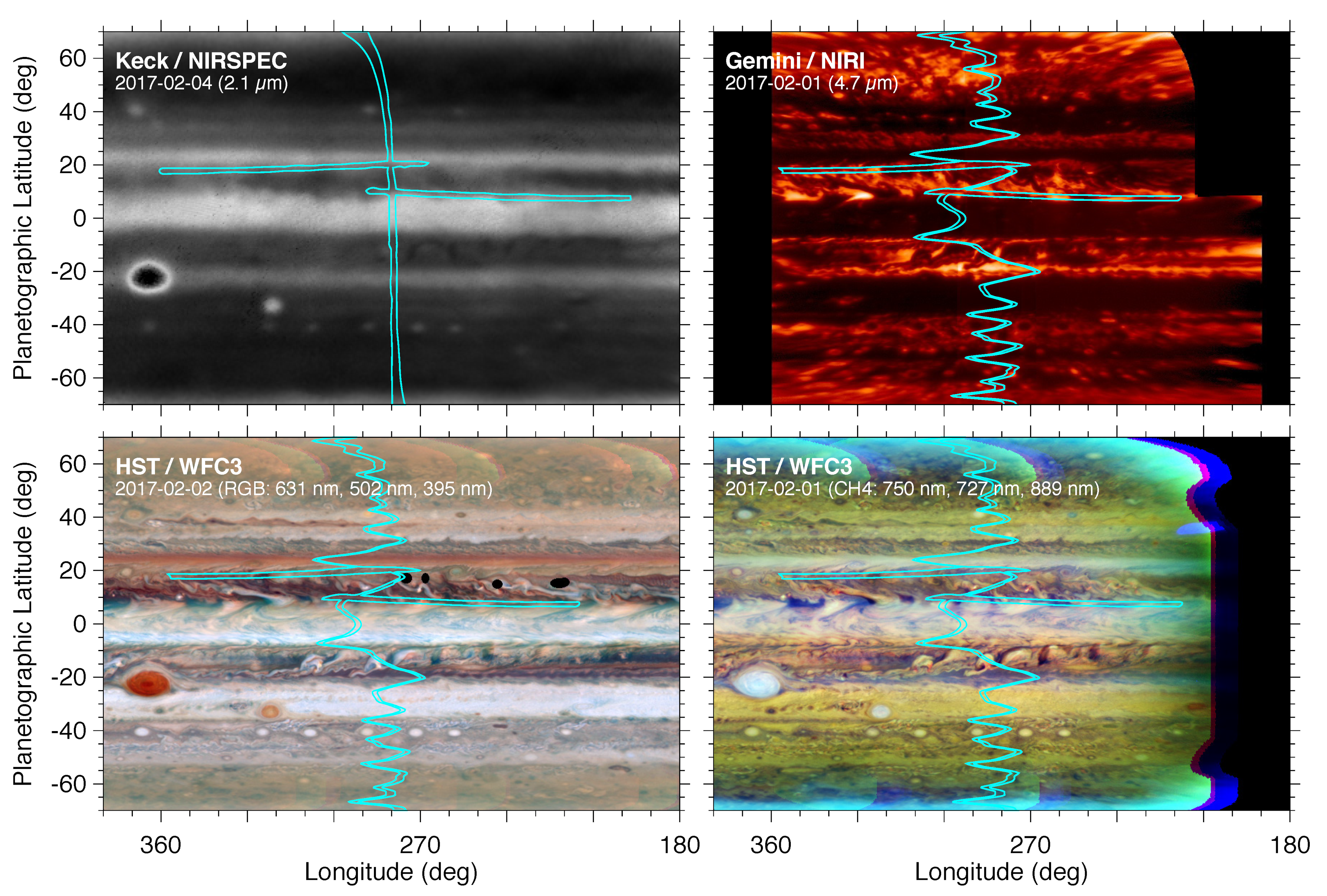
The spectral data were navigated using images of Jupiter in reflected near-infrared (NIR) sunlight at 2.1 µm acquired with the slit viewing camera (SCAM) on NIRSPEC (see Figure 1, top left). Our observing approach interleaved Jupiter spectral frames (A), background sky spectra (B), and NIR images (C) in a BCACB sequence. Each cycle took about 8 minutes to complete, with total integration times of 1 s for each C-frame and 1 min for each spectral frame.
Including offsets and filter changes, the duty cycle had about a 13% on-target time for each Jupiter spectrum; however, our priority was maximizing the accuracy of the spatial navigation and background subtraction. Jupiter ranged from airmass 1.8 to 1.2 over the observation window. We aligned a latitude/longitude grid to the limb of the planet for each C-frame, with the A-frame navigation solution derived by assuming a linear telescope drift between adjacent C-frames (and accounting for planetary rotation in the 2–3 min interval between images).
The spatial registration was refined by matching the continuum brightness of the spectrum at each pixel with 5 µm images of Jupiter (see Figure 1, top right) acquired using the Near Infrared Imager (NIRI) on the Gemini telescope [7]. Since the NIRI images were acquired 3 days before the spectra, it was necessary to use zonal wind profiles [8] to calculate the predicted cloud locations at the time of the spectra. This is denoted using a wavy north–south profile (double cyan lines) to indicate which cloud features would be visible from our slit considering the time interval between the NIRI and Keck data.
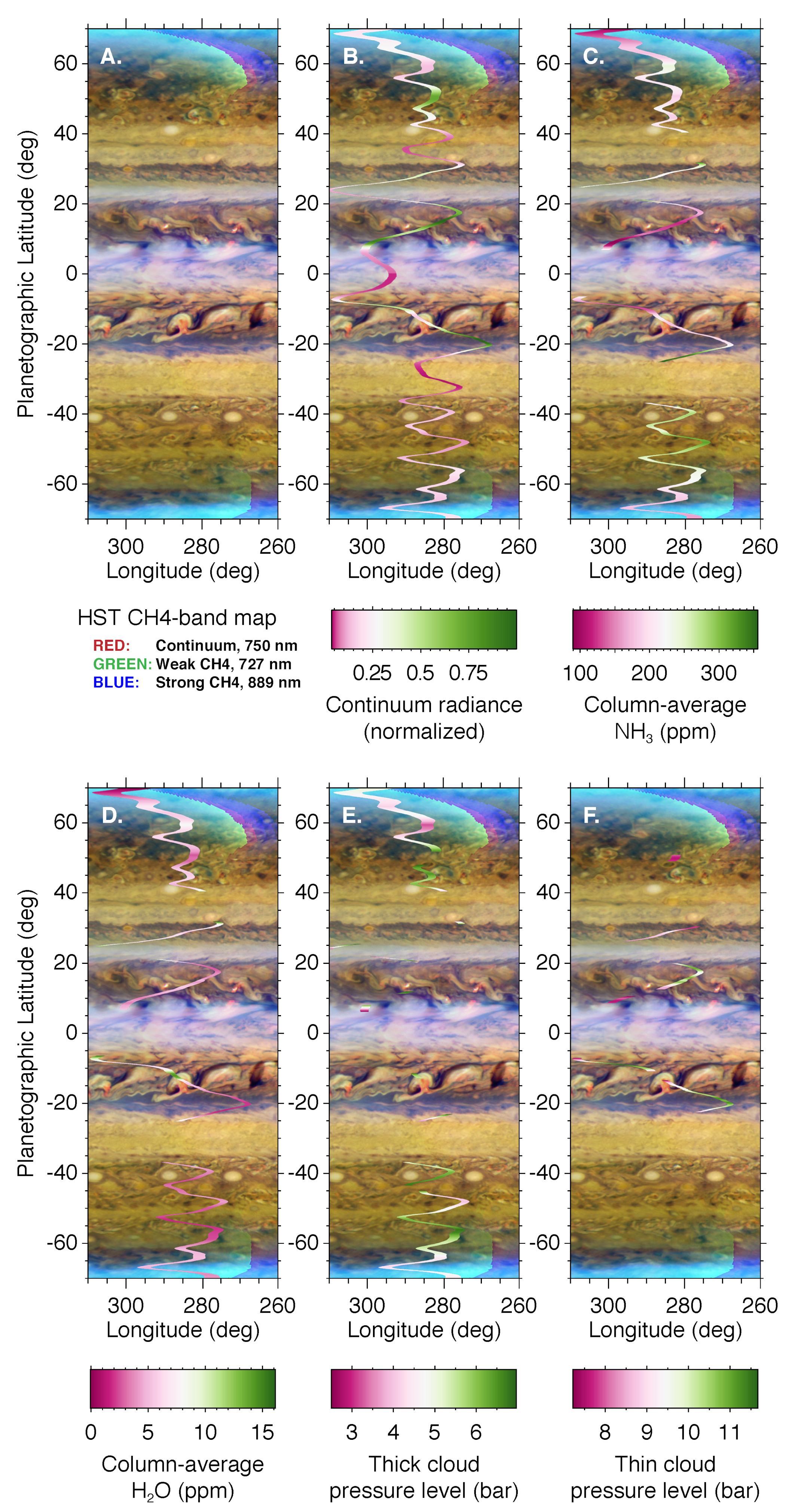
Hubble Space Telescope images using the WFC3 camera were also acquired at visible wavelengths (Figure 1, bottom left) and in three CH bands in the NIR (Figure 1, bottom right). Methane-band imaging permits the determination of cloud heights, and it may constrain their composition (e.g., ammonia or water ice) using equilibrium cloud models [7]. All of these images are displayed in the form of cylindrical maps in Figure 1.
3. Data Analysis and Results
3.1. North–South Variation in the Deep Cloud-Top Pressure
The band pass that we use to derive the cloud structure at 4.66 µm contains absorption lines of deuterated methane (CHD). Methane and its isotopologues are well mixed: they do not condense, nor are they destroyed photochemically in Jupiter’s troposphere at the altitudes probed in this study. We therefore assume that CH and CHD have a constant mixing ratio with respect to H in Jupiter’s troposphere. Thus, variations in the strength and shape of the CHD lines between different locations on Jupiter must be due to changes in the cloud structure—not the gas concentration.
Bjoraker et al. [9] introduced the idea of using CHD absorption to study Jupiter’s deep cloud structure. Extrema in CHD were identified, and radiative transfer models were calculated for a Hot Spot in the South Equatorial Belt (SEB) at 17S and a cloudy region in the South Tropical Zone (STZ) at 32S. Although measurements were acquired covering 70S to 70N in our previous study, it was not practical to model every latitude. The current study extends this analysis by converting the CHD absorption into the cloud-top pressure for each spatial pixel along the slit, which then can be used to investigate the cloud structure and volatiles at all latitudes rather than being limited to selected locations.
We generated synthetic spectra of Jupiter at 5 µm to model the NIRSPEC data. These spectra were calculated using the Spectrum Synthesis Program (SSP) radiative transfer code first described in [10] and updated in Bjoraker et al. [11]. The input temperature profile was obtained from the Galileo Probe [6]. Although this profile pertains only to the Probe Entry Site, it can be used elsewhere on Jupiter for this study because the shapes of the absorption features at 5 µm are only weakly dependent on the temperature. The line parameters for CHD and other 5 µm absorbers are from GEISA 2003 [12]. The parameters for CHD-H and CHD-He broadening have been measured in the lab [13,14,15]. We used a broadening coefficient of 0.0613 cm /atm (296/T) for CHD colliding with a mixture of 86.3% H and 13.6% helium, as measured by the Galileo Probe [16]. Pressure-induced H coefficients were obtained using laboratory measurements at 5 µm in [17] and the formalism developed in [18].
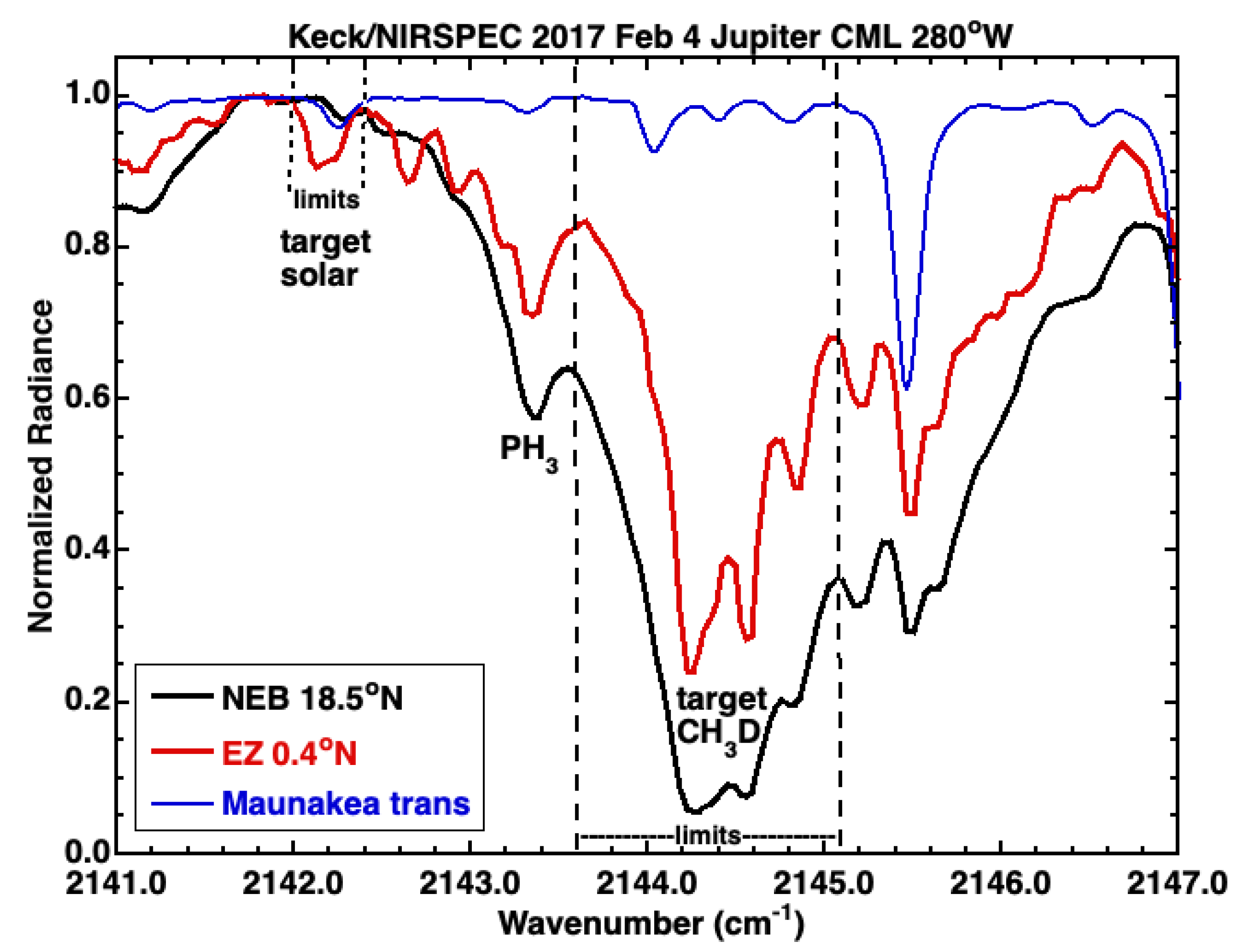
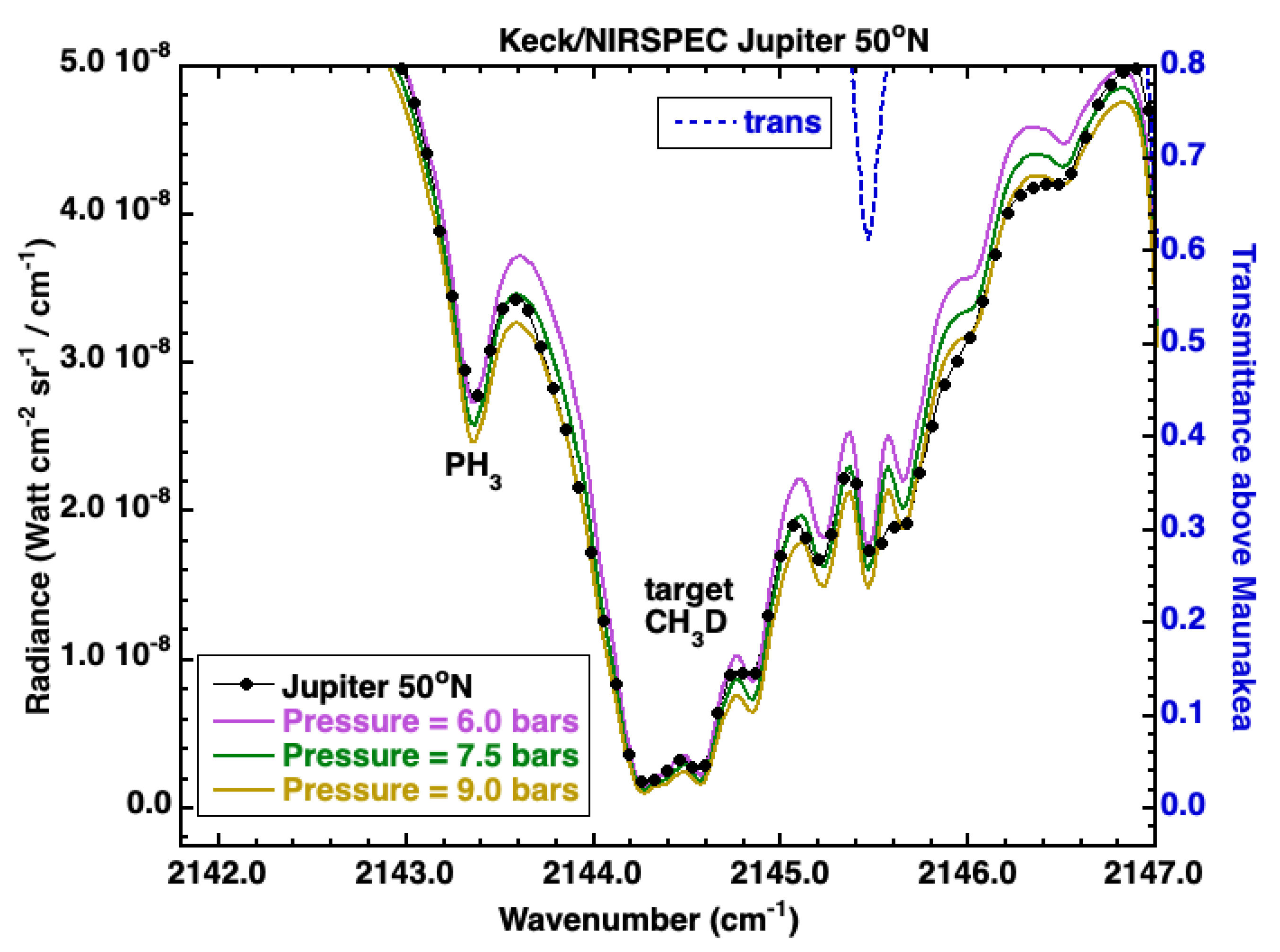
Figure 2 shows NIRSPEC spectra at 4.66 µm (2141–2147 cm) in which the slit was aligned north–south on the central meridian covering Jupiter’s northern hemisphere. Spectra were normalized at 2141.8 cm to permit comparisons of the line shapes. Note the large change in the appearance of CHD lines at two different latitudes along the slit. The set of CHD absorption lines near 2144 cm are stronger and broader in the NEB at 18.5N due to a combination of opacity and pressure broadening. We calculated the equivalent width (defined below) of the CHD feature as a function of spatial pixels over the spectral range from 2143.62 to 2145.10 cm. This provides important clues to the deep cloud structure.
We also analyzed a nearby Fraunhofer (solar) line due to CO in the Sun. The scattered solar flux is much smaller than Jupiter’s thermal emission in most regions, only becoming visible in the cloudiest areas. Thus, the Fraunhofer line is observed only in zones, such as the EZ at 0.4N and not in the NEB at 18.5N. We measured the spatial variation of the strength of this line on Jupiter over the spectral range from 2141.97 to 2142.37 cm, as shown in Figure 2. This provides information on the amount of reflected sunlight in the spectrum, as described below. This same Fraunhofer line was used by Bjoraker et al. [9] to model the STZ at 32S.
The equivalent width (EW) is a measure of the spectral line strength and is defined as the area of the spectral feature relative to a normalized continuum. The nomenclature arises when considering the width of a rectangular absorption feature from the continuum to zero that has the equivalent area of the spectral line [19]. The EWs of the CHD feature and the targeted Fraunhofer line as functions of the spatial pixels were calculated numerically using the trapezoid rule.
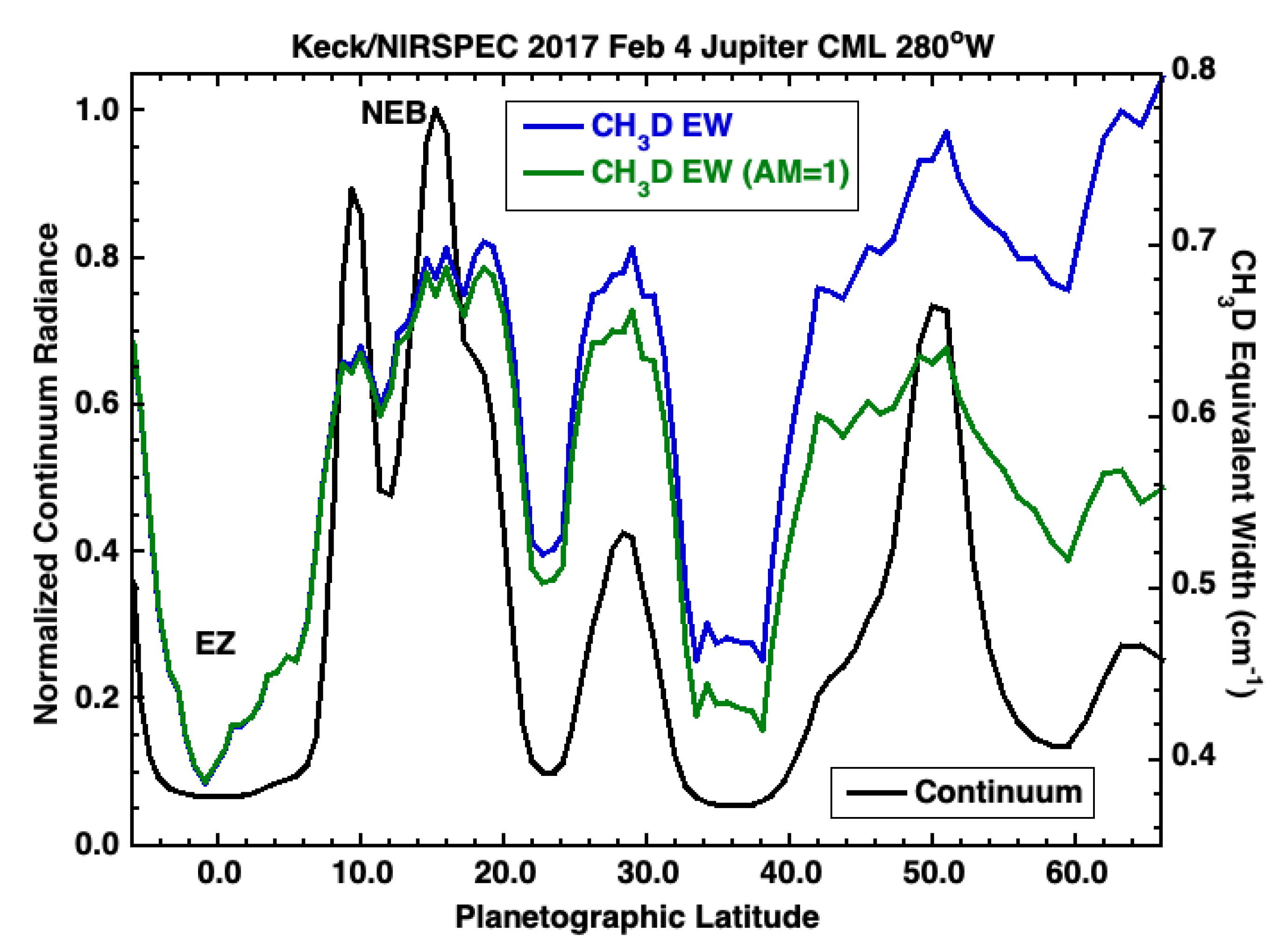
In Figure 3, the EW of the targeted CHD absorption feature is shown as a function of latitude between 6S and 66N along Jupiter’s central meridian. The EW along the line of sight was corrected to normal viewing using the Jovian airmass. Since this feature is optically thick and, therefore, is on the nonlinear portion of the curve of growth, it was necessary to use a power-law relation obtained from our radiative transfer code developed to model Jupiter at 5 µm [9,11]. The EW at Jupiter airmass () of 1 can be calculated from the EW at values of between 1 and 1.7 using the following relation:
This power law was evaluated for a cloud-free model atmosphere with an opaque lower boundary at 6.5 bar, simulating a water cloud. In the model, the CHD mole fraction was 0.18 ppm [20]; the HO mole fraction at 6.5 bar was 4 ppm, an intermediate value between the retrieved values ranging between 1.5 and 14 ppm; and PH was 0.6 ppm [9]. This model is an approximation as HO varies spatially on Jupiter, and the wings of these absorption features act as a continuum absorber to affect the strength of the CHD feature.
As discussed in Section 3.2, the retrieved cloud-top pressures in belts and Hot Spots should be reliable for HO mole fractions in the 1–15 ppm range for p > 5 bar. Regions with low values of CHD EW are identified as containing water clouds, which, in turn, may also have much larger gaseous HO abundances (∼1000 ppm) for p > 5 bar. As a result, this technique may be used to identify the spatial location of water clouds but the cloud-top pressures will be overestimated.
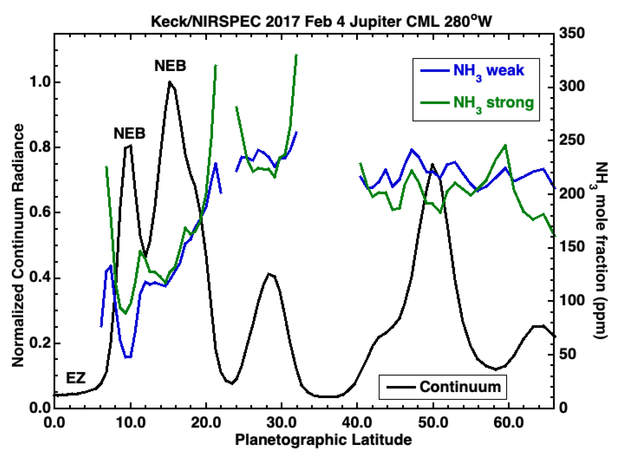
The value of EW corrected for airmass correlates well with the normalized continuum radiance—also shown in Figure 3. The continuum radiance depends on the transmission of both upper and lower clouds. As shown below, the CHD EW depends primarily on the opacity of the lower clouds. This suggests that much of the variation of the continuum brightness at 5 µm between belts and zones on Jupiter can be attributed to deep clouds.
The EW (corrected to normal viewing) of the targeted CHD absorption feature was converted to the cloud-top pressure using our radiative transfer model with different input parameters. A pair of models was constructed for a Jovian airmass of 1 with opaque lower boundaries at 4 and 10 bar. The gas composition for each model was the same as in the airmass study described above. The CHD EW over the targeted spectral interval was measured for both models. A power law was calculated to interpolate EW values between pressures (p) of 4 and 10 bar.
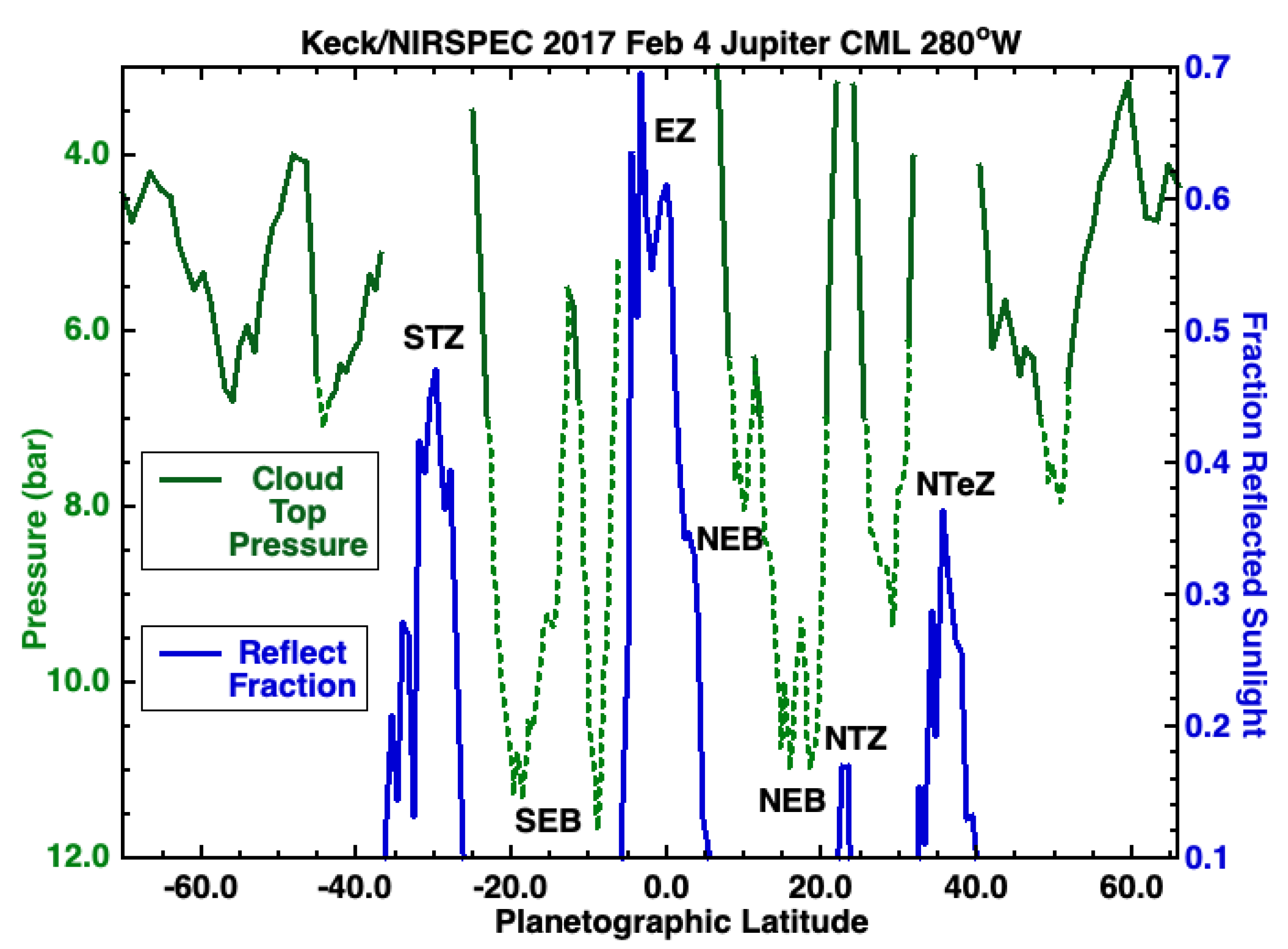
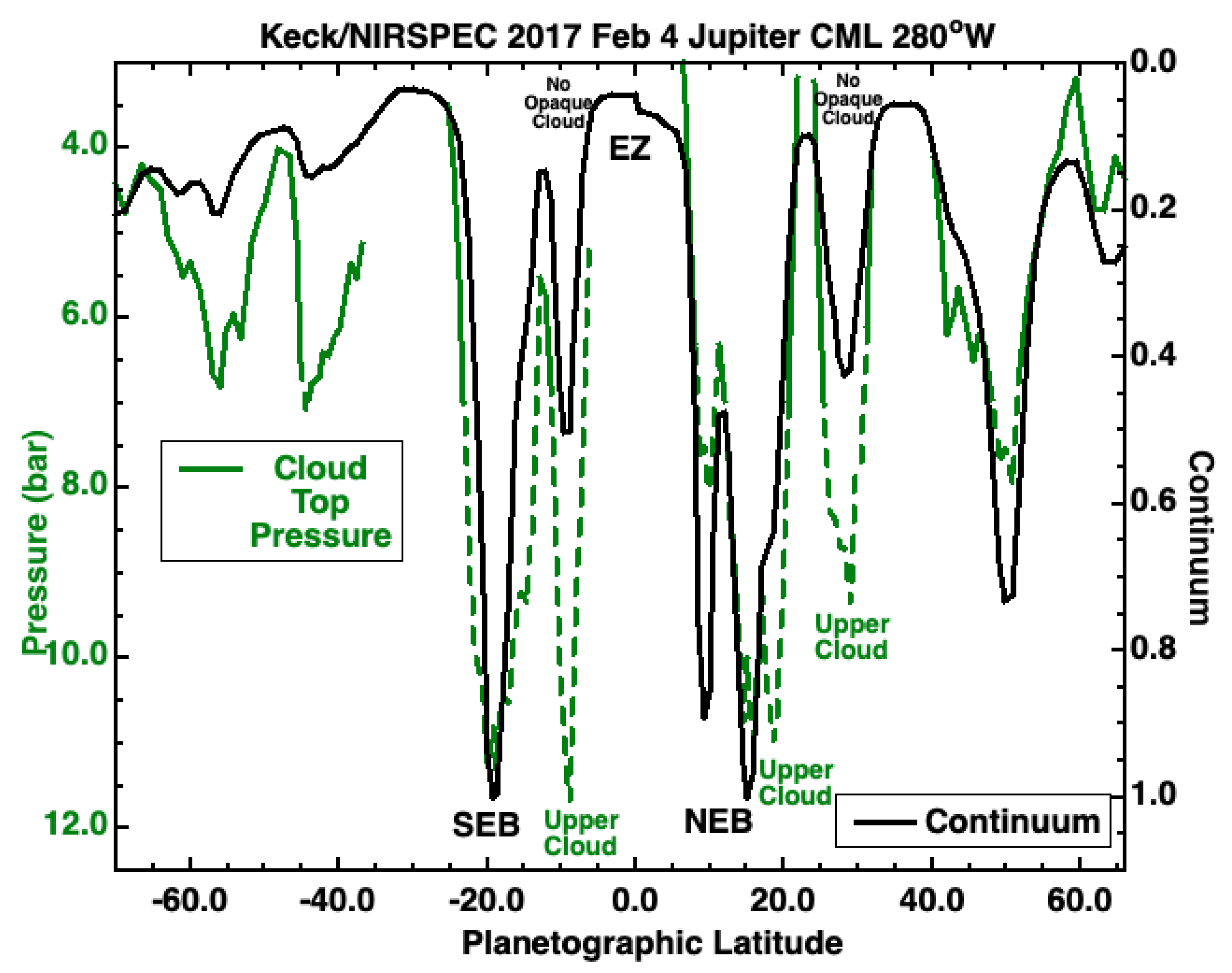
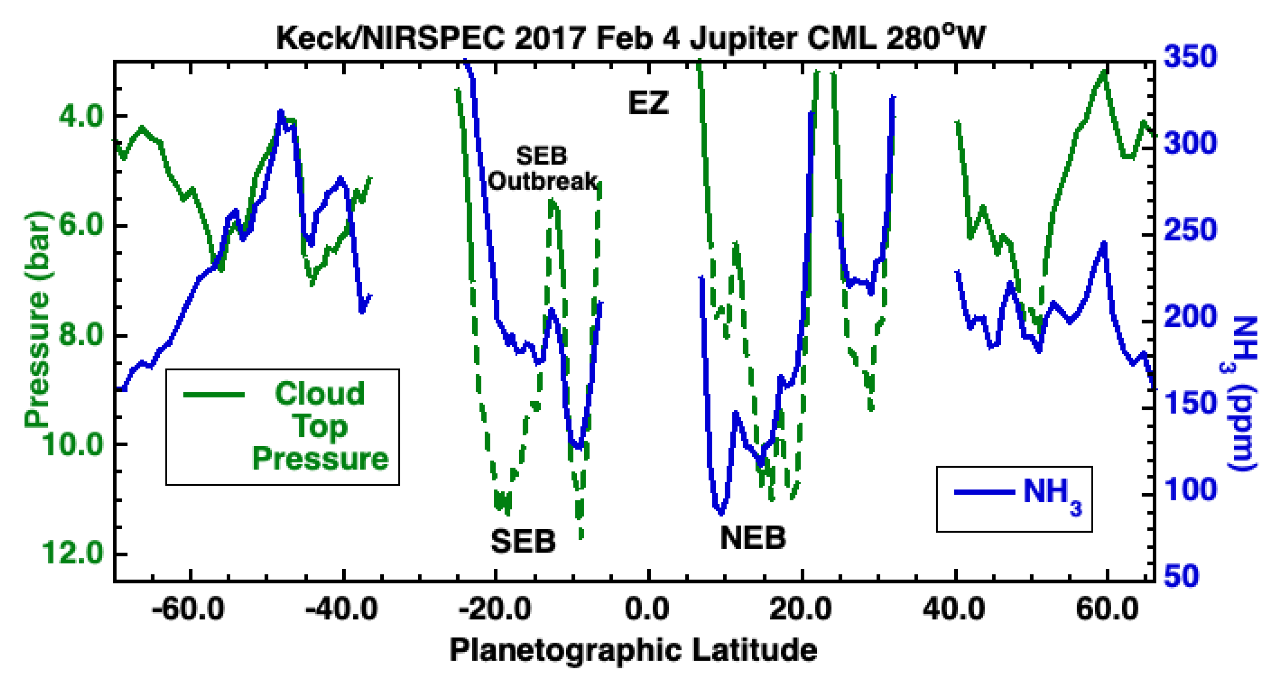
The corresponding pressure of the opaque lower boundary is shown in Figure 4 as a function of latitude between 70S and 66N. An important point to note is that an opaque boundary at 11 bar, caused primarily by gas opacity, is indistinguishable from a 20 bar cloud boundary. That is, collision-induced absorption due to H-H, and H-He, combined with opacity from the wings of HO and other molecules limits the line formation region at 4.66 µm to pressures less than 11 bar. Thus, the apparent cloud-top pressure of 11 bar in the NEB and SEB shown in Figure 4 is not a real cloud. It is a region of maximum CHD EW, which we interpret as due to the absence of opaque clouds at pressures less than 11 bar at these locations.
This coincides with the highest continuum radiance, as shown in Figure 3 for the NEB. Although the CHD EWs are identical for the 11 bar and 20 bar cases, the CHD EW for a 7 bar cloud is 10% less than for the 11 bar case. The Keck data have sufficient signal-to-noise to distinguish between regions with an opaque cloud at 7 bar and areas that lack deep clouds. However, regions denoted in Figure 4 as having clouds deeper than 7 bar may have optically thin clouds between 4 and 7 bar rather than, for example, an opaque cloud at 8 bar. Thus, apparent cloud-top pressures >7 bar are shown as dashed lines to indicate thin clouds or, in the case at 11 bar, no deep clouds at all.
The spectrum at 4.66 µm provides valuable information on the ratio of reflected sunlight to thermal emission on Jupiter, which is critical for understanding Jupiter’s cloud structure. We compared the equivalent width of the Fraunhofer line at 2141.8 cm (Doppler shifted to 2142.2 cm) with its measured value in the Sun using ATMOS data [21,22]. Fraunhofer lines on Jupiter are due to sunlight reflecting off of upper clouds. They are not observed in belts or Hot Spots because these regions are dominated by thermal emission. The ratio of the Jovian EW to the solar value is interpreted as the ratio of reflected sunlight to the sum of the reflected solar and Jovian thermal emission.
This value (shown in Figure 4) is significant in the EZ and other zones but negligible in the belts. We interpret high values of reflected sunlight as due to two factors: the presence of upper clouds that reflect sunlight (likely NH ice clouds near 0.6 bar as inferred in the Great Red Spot by Bjoraker et al. [11]) as well as opaque clouds near 4 bar that block the thermal radiation originating from deeper levels. Reflected sunlight also affects the slope of Jupiter’s continuum between 4.6 and 5.4 µm; however, this effect may be difficult to distinguish from wavelength-dependent cloud absorption.
Figure 4 presents evidence for opaque clouds between 3 and 7 bar, which we interpret as due to water clouds. Water clouds are present at many latitudes, including 65S, 50S, 13S, and 60N. Other latitudes (30S, the Equator, 23N, and 35N) are inferred to have water clouds that attenuate thermal emission sufficiently to result in a significant amount of reflected sunlight. These include the South Tropical Zone (STZ), Equatorial Zone (EZ), North Tropical Zone (NTZ), and North Temperate Zone (NTeZ). We do not show cloud-top pressures in the EZ and the other zones in Figure 4.
The presence of reflected sunlight affects the EW of CHD in a way not described in Equation (2), which assumes 100% thermal emission. As a result, we cannot rule out the possibility that the zones shown in blue have thick NHSH and NH clouds rather than water clouds. However, detailed modeling of the STZ at 32S by Bjoraker et al. [9] using the entire 5 µm spectrum, rather than only the EW of CHD, required an opaque cloud top between 4 and 5 bar—consistent with a water cloud. In addition, by analogy with the Great Red Spot, the zones denoted in blue (with significant reflected sunlight) likely have all three cloud layers as described in [11].
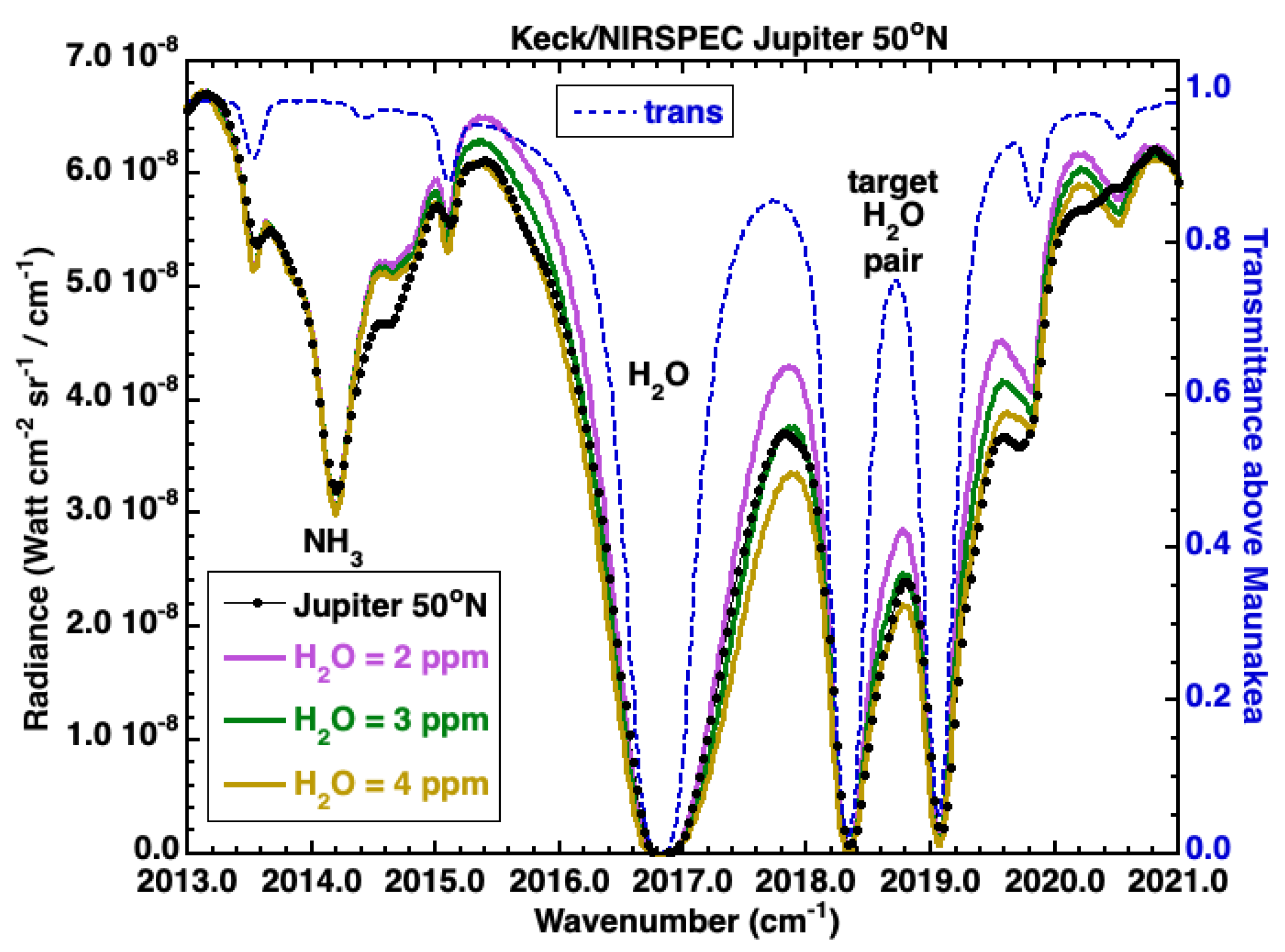
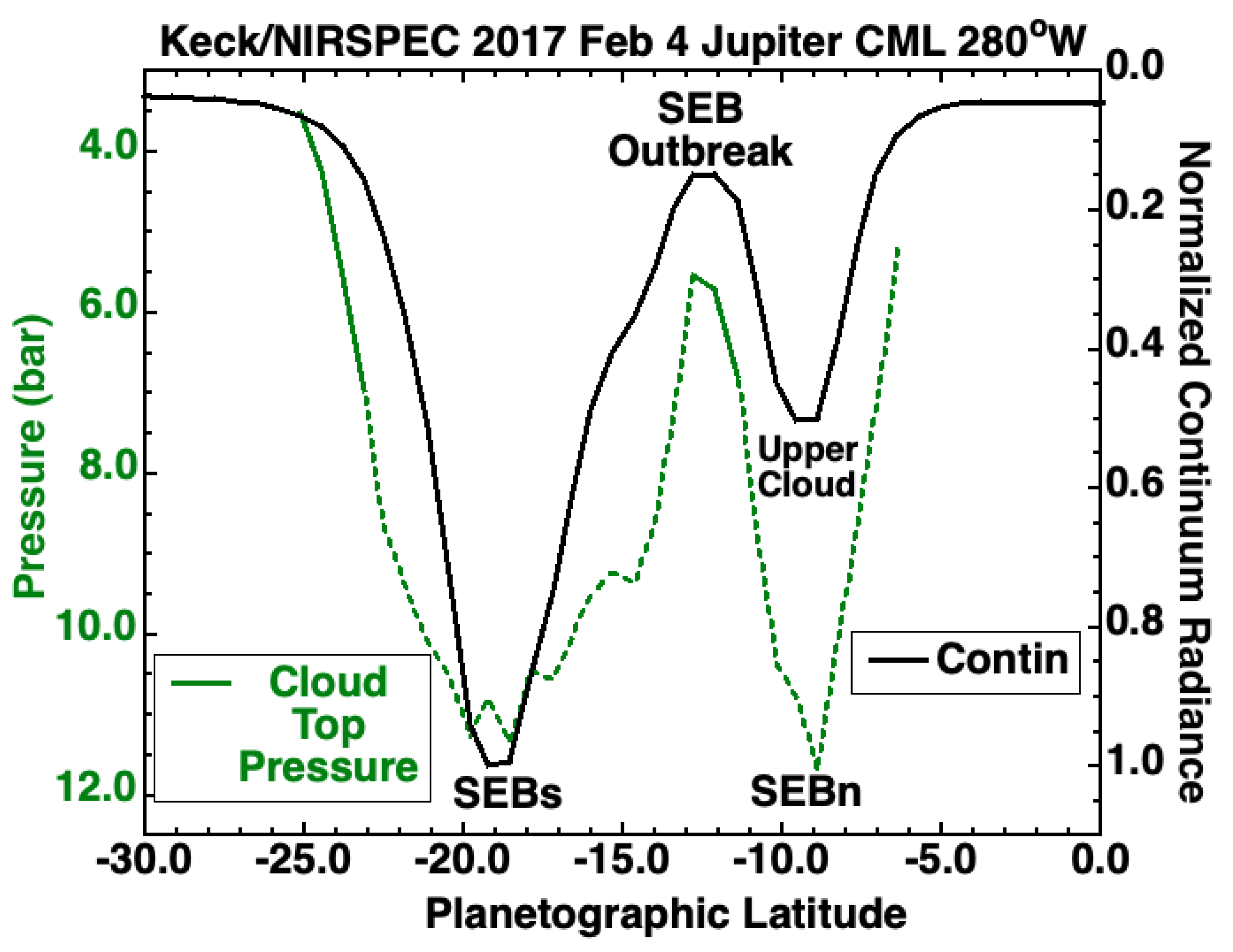
In Figure 5, we compare the spectrum of Jupiter at 50N with three radiative transfer models in which the cloud-top pressure varied between 6 and 9 bar. The best fit to CHD was provided by the model with the cloud top at 7.5 ± 0.5 bar. In Figure 6, the pressure of the lower boundary and continuum radiance are shown as functions of latitude between 70S and 66N. This is a composite of data from two slit positions that each span one hemisphere. The values of the cloud-top pressure are the same as in Figure 4. The continuum radiance was normalized to one in each hemisphere. The South Equatorial Belt (SEB) at 20S exhibits maxima in both continuum radiance and CHD EW, indicated by an apparent cloud at 11 bar; i.e., this region is thus free of deep clouds. Other latitudes (e.g., 25–70S) have thick water clouds.
Imaging of Jupiter at 5 µm shows large variations in continuum radiance due to the combined transmission of all clouds at pressures less than 11 bar. However, it has been difficult from 5 µm imaging alone to separate upper clouds (0.5 to 2 bar) from lower clouds (3 to 7 bar). By combining the continuum radiance with CHD EWs, we can find regions that have upper clouds but lack deep clouds. Figure 6 provides evidence for upper clouds at 10S, 19N, and 28N. This comes from measured high values of CHD equivalent width (plotted as a dashed line and interpreted as free of deep clouds) and relatively low continuum radiance.
This low radiance must be due to thick but not opaque upper clouds. The upper clouds may be composed of NH ice, NHSH, or both. Our technique is sensitive to the temperature of the absorbing clouds. Upper clouds with temperatures of 150 to 200 K attenuate thermal emission from below; however, they emit a negligible amount at 5 µm compared with opacity sources at 5 bar where the T is 273 K. Thus, cold upper clouds at 10S (for example) do not affect the EW of CHD, while warm water clouds at 13S do. Observations of Jupiter in reflected sunlight show the presence of upper clouds at latitudes other than the ones highlighted here. The ability to distinguish upper clouds from water clouds using 5 µm data alone is new.
A quantitative estimate of the transmission of upper clouds is only possible at locations with high values of CHD EWs. At latitudes with low CHD EW (cloud-top pressures 3 to 7 bar), the continuum radiances are low due to the presence of deep clouds. There is evidence for upper clouds in regions with significant reflected sunlight, as shown in Figure 4; however, it is difficult to measure the transmittance of each cloud layer separately.
Figure 6 also shows latitudes that exhibit the opposite relation between the continuum brightness and CHD EW. At 10N and 50N, high continuum levels indicate a high combined transmittance for all cloud layers despite the presence of optically thin water clouds between 4 and 7 bars. We interpret this as evidence for exceptionally transparent upper clouds at these locations. Observations at visible and near-IR wavelengths would be needed to test this conclusion.
3.2. North–South Variation in the Ammonia and Water Abundances
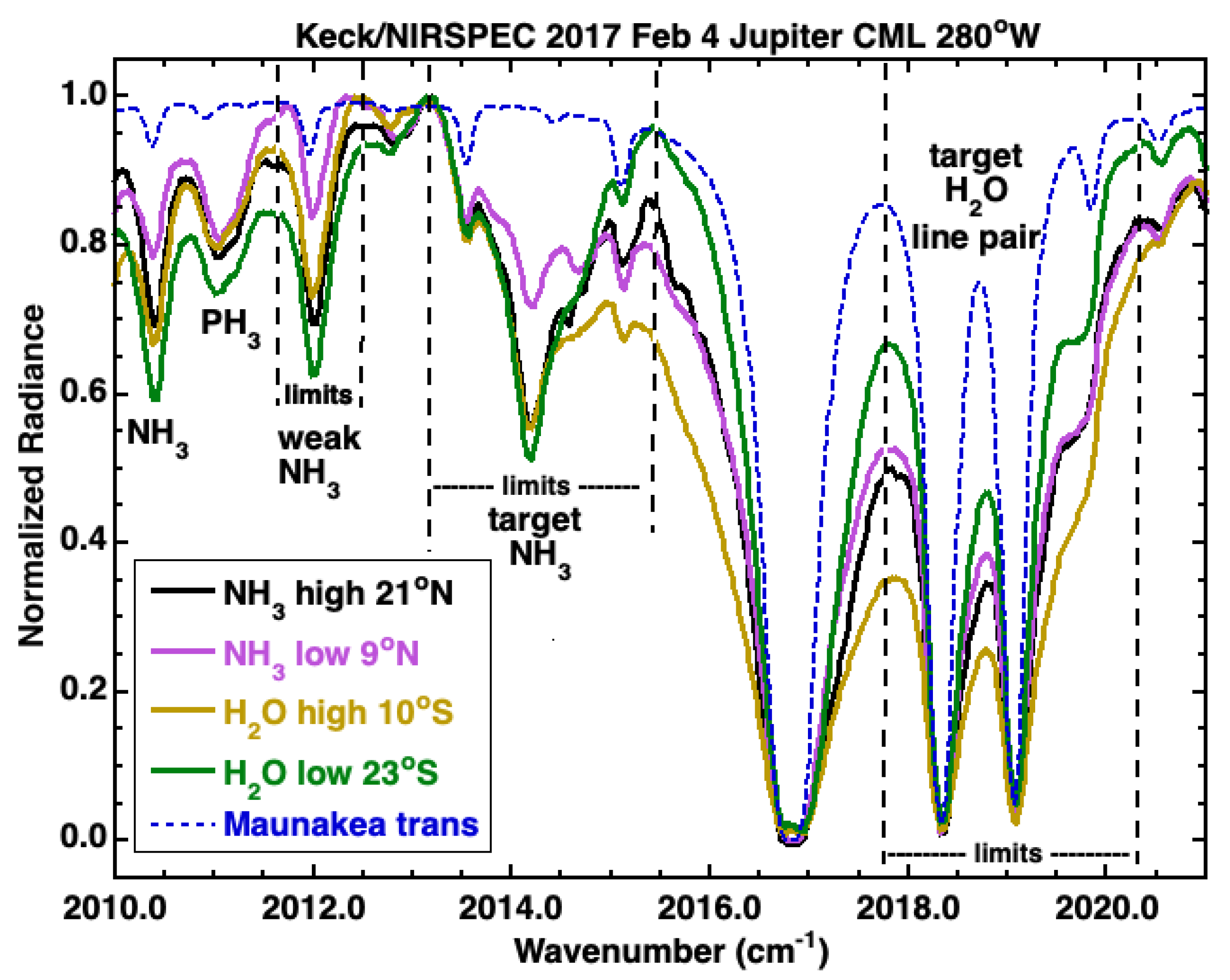
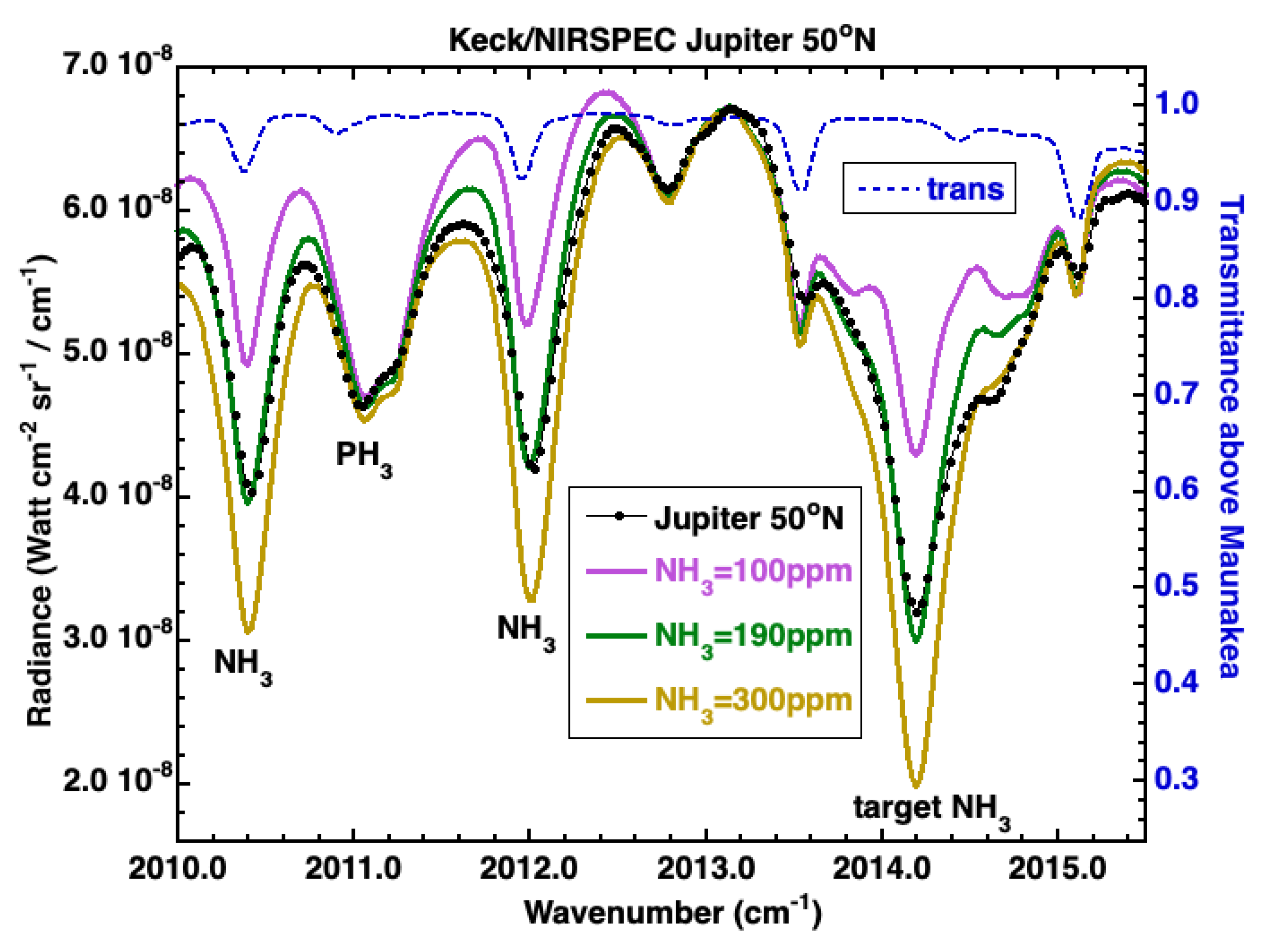
Figure 7 shows NIRSPEC spectra at 4.96 µm (2010–2021 cm) obtained from two slit positions that were aligned north–south on the central meridian to cover Jupiter’s northern and southern hemispheres. The spectra were normalized at 2013.16 cm to permit the comparison of line shapes. A strong NH feature at 2014 cm was used to derive the ammonia abundances.
The weaker NH line at 2012 cm was investigated as well. Equivalent widths were calculated for the target line at 2014 cm using the frequency limits (2013.16 to 2015.37 cm ) shown in Figure 7. Equivalent widths were also calculated for the weaker NH line between 2011.62 and 2012.50 cm. The ammonia mole fraction was retrieved using both frequency ranges for one test case yielding similar abundances; however, ultimately, we used the stronger NH feature at 2014 cm for our Jupiter analysis.
Information about Jovian HO comes primarily from the wings of three strong absorption features centered between 2016 and 2020 cm. Their cores coincide with strong telluric lines; however, the Jovian lines are broader than their terrestrial counterparts. The limits for the HO line integration include telluric absorption but this component was subtracted out using the model shown in blue. After several iterations, we used the pair of HO lines between 2017.83 and 2020.24 cm and excluded the strongest line at 2017 cm. The use of this optically thick line pair enabled our radiative transfer model to convert the EW to the HO mole fraction. Note the exceptionally broad wings of the HO feature at 10S between 2015 and 2016 cm and between 2019 and 2020 cm.
A comparison between Figure 7 and Figure 4 and Figure 6 indicates that the extrema in the depths of absorption lines of NH and HO do not match the extrema in CHD, which we used to derive the deep cloud structure. For example, the ammonia absorption is low at 9N despite the lack of deep clouds at this latitude. This indicates a real depletion in NH rather than a shorter absorption path length. Similarly, HO exhibits large changes in the wing absorption between 2015.5 and 2016 cm between 10S and 23S, despite the lack of deep clouds at these locations. This represents a real variation in the mole fraction of HO between 3 and 6 bar where the targeted absorption features in Jupiter’s atmosphere sound, as discussed below.
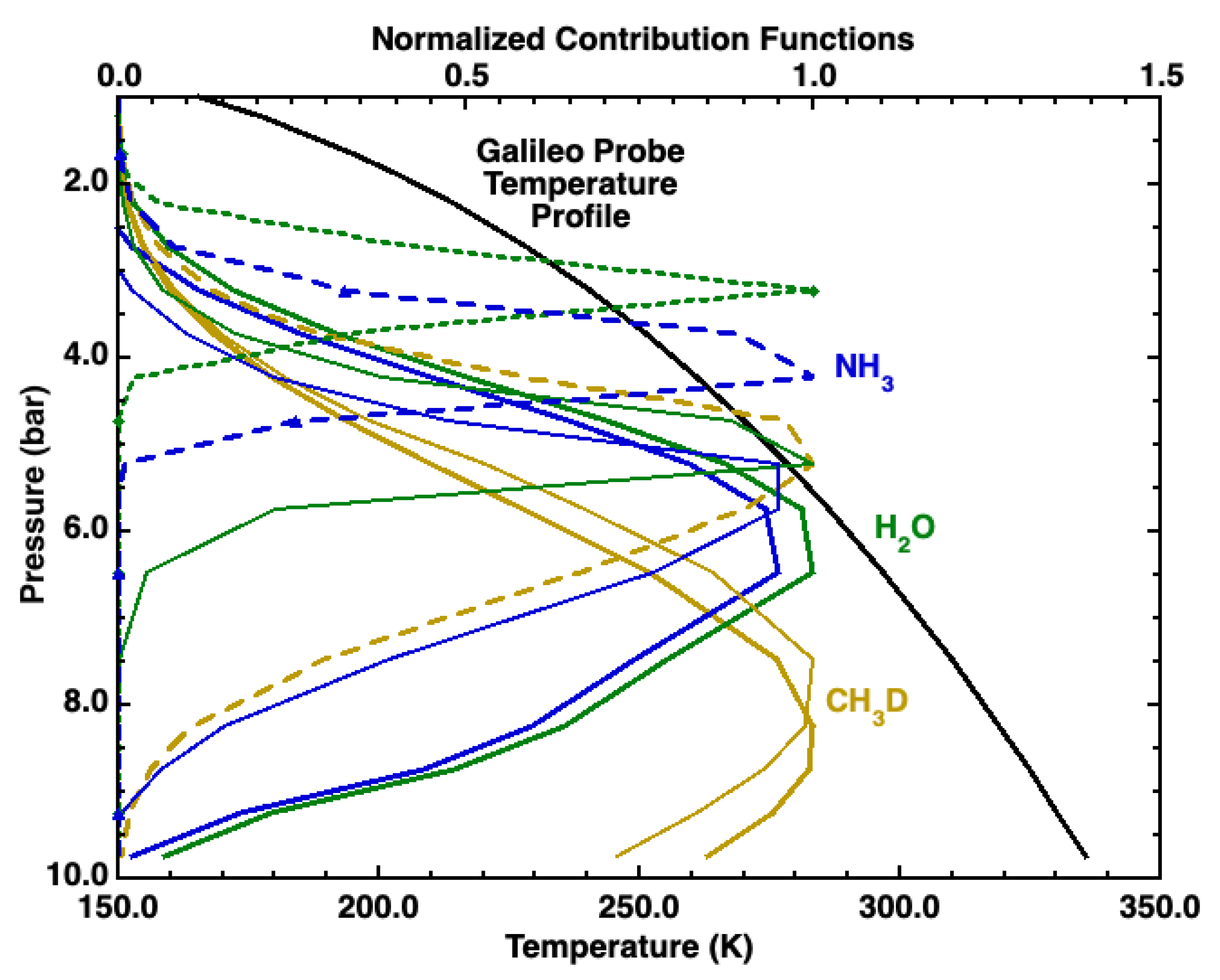
In Figure 8, we show the Galileo Probe temperature profile used for all latitudes along with normalized contribution functions for the targeted absorption lines in this study. Contribution functions for each molecule were calculated for three different abundances of HO: 4, 47, and 1000 ppm for p > 5 bar. The retrieved parameters in this study assumed 4 ppm HO, which provided a better fit to the targeted HO line pair in belts and Hot Spots. A value of 47 ppm was investigated to match the Galileo Probe value measured at 11 bar [23]. This value was assumed in our previous study [9].
Using this HO abundance instead of 4 ppm shifts each contribution to higher altitudes or to lower pressures by 0.5 to 1 bar. The largest change occurs for a deep value of 1000 ppm HO. Contribution functions peak for CHD, NH, and HO at 5 bar, 4 bar, and 3 bar, respectively. As a result, low values of CHD equivalent width may still be used to identify the spatial locations of water clouds. However, the retrieved cloud-top pressures in these regions will be overestimated if water clouds are accompanied by large values of gaseous HO below their cloud tops, as is likely to be the case. Since the retrieved NH and HO mole fractions depend on the derived cloud-top pressure, the values reported below in regions with water clouds will be underestimated.
All contribution functions pertain to a cloud-free model atmosphere at normal incidence with an opaque boundary at 10 bar. For our assumed HO abundance of 4 ppm for p > 5 bar, both NH and HO peak near 6 bar, while CHD exhibits a peak near 8 bar. These functions will shift to lower pressures at higher emission angles and after the inclusion of the optically thin cloud opacity. An opaque cloud truncates each function at the designated cloud pressure. The atmospheric profiles in our model are truncated at this altitude, and an opaque “surface” temperature equivalent is inserted.
The relation between NH EW and NH mole fraction was established by modeling regions at 50N and at 56S (not shown), using our radiative transfer code. These latitudes were chosen to avoid strong gradients in the cloud-top pressure or extreme heterogeneity, as in the NEB. The Jovian airmass at 50N was 1.68, and the deep cloud-top pressure was 7.5 bar, derived from CHD as shown in Figure 5. The best fit model to this latitude required 190 ± 20 ppm NH, as shown in Figure 9. This fit made use of NH absorption features at 2010.4 and 2012.0 cm, in addition to the target line at 2014.2 cm. This value is in excellent agreement with the NH abundance at this latitude derived from microwave observations of Jupiter using the Very Large Array (VLA) [24].
The ammonia mole fractions at all locations were obtained using three power laws to convert measured EWs to NH mole fractions. This required three steps. First, the EW at the observed Jovian airmass was converted to a value for the unit airmass (emission angle of 0). The airmass power law was obtained by calculating the EWs for synthetic spectra with 215 ppm NH, cloud-top pressure of 6.8 bar, and Jovian airmasses of 1.0 and 1.7. The latter case matches the conditions for a Jupiter spectrum at 56S and is similar to conditions at 50N at the same airmass. Next, a pressure power law was obtained by calculating the EWs for synthetic spectra with 215 ppm NH, airmass of 1, and cloud-top pressures of 4 and 10 bar. Using the measured EWs for NH converted to unit airmass, the cloud-top pressures derived from CHD, and the pressure power law, we calculated the NH EW for a cloud-top pressure of 6.5 bar.
In the last step, a mole fraction power law was obtained by calculating the EWs for synthetic spectra with airmass of 1, a cloud-top pressure of 6.5 bar, and NH mole fractions of 200 and 340 ppm. Finally, the measured EW for each spatial pixel, after conversion to the unit airmass and a cloud-top pressure of 6.5 bar, was converted to the NH mole fraction.
In Figure 10, we compare the derived NH mole fractions for Jupiter’s northern hemisphere using two frequency ranges covering the weak 2012 cm line and the strong NH line at 2014 cm. Both frequency ranges have their own set of three power laws. Most latitudes have NH in the 150–300 ppm range as measured above the top of an opaque lower cloud except for a significant depletion in the NEB near 10N. We find similar spatial variations in NH mole fractions using the two different spectral ranges.
This figure illustrates that the accuracy of our retrieved NH is not solely determined by the S/N ratio, which is high for all spatial pixels. Instead, it depends on systematic factors, such as the accuracy of the power laws, the choice of continuum frequencies, the degree of blending with other molecules, and the fraction of reflected sunlight. The mole fractions derived from both NH features critically depend on the cloud pressures derived from CHD. In general, the spatial variation of NH should be robust as it is based on the measured equivalent widths.
The absolute NH abundances, however, are model-dependent with the largest uncertainty in regions with HO clouds. The ammonia abundances are not shown in regions where the fraction of reflected sunlight exceeds 0.1. Ultimately, we adopted values derived from the strong NH feature at 2014 cm. The difference between the two models is a better indication of the retrieval error than the Keck signal-to-noise ratio, which is high at all latitudes.
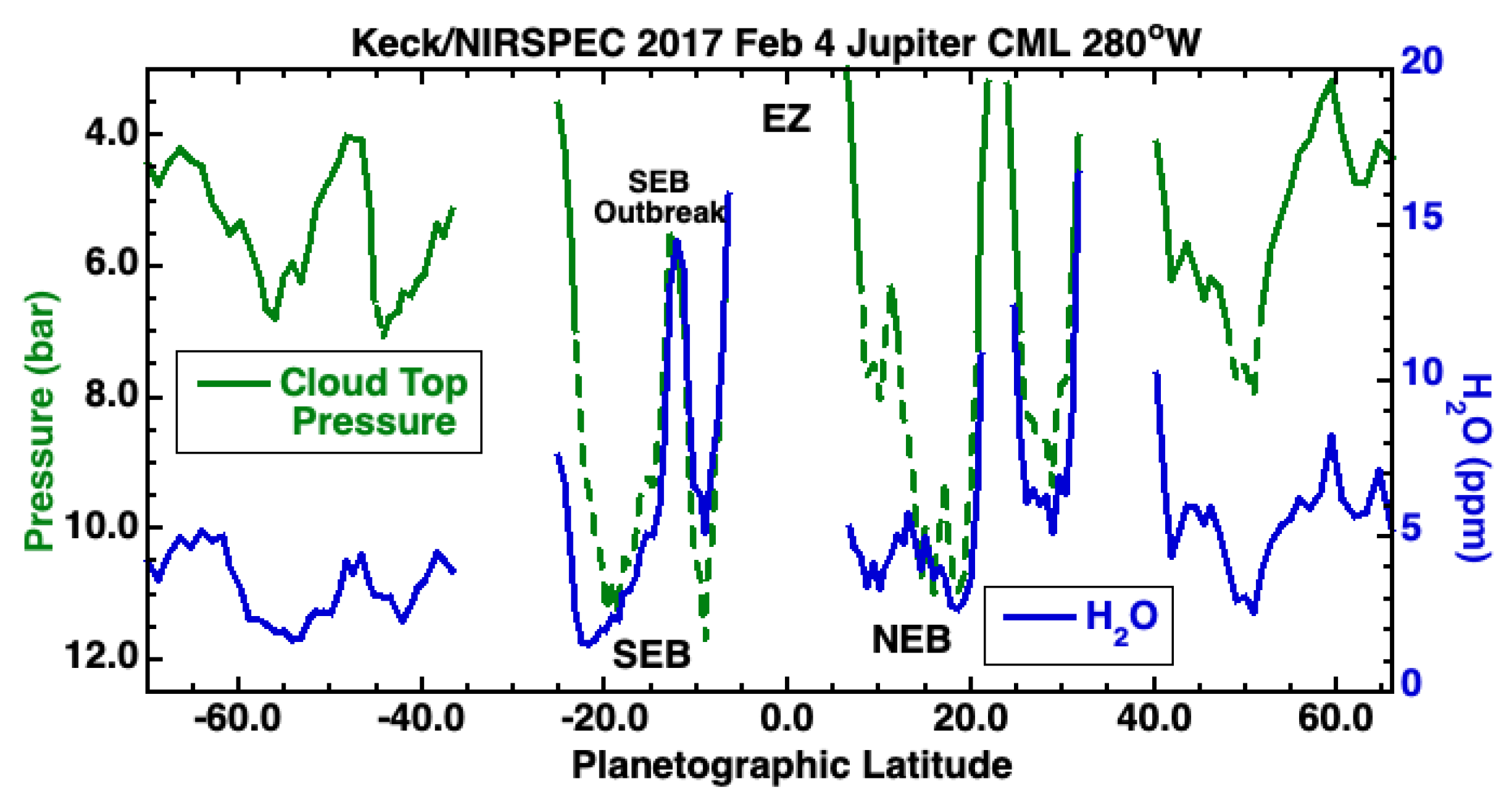
In Figure 11, we show the mole fraction of NH as a function of latitude between 70S and 66N. All values pertain to a column above an opaque lower boundary, denoted as the cloud-top pressure, derived from CHD. The vertical profile is constant for p > 0.7 bar and follows the saturated value at p < 0.7 bar. The retrieved abundances are in the 150–300 ppm range, except for the NEB. There is a strong latitudinal gradient in NH from a minimum of 90 ppm at 10N to 200 ppm at 20N.
There is evidence for a decrease in NH in the NEB for p < 1.8 bar from the infrared spectra at 5.32 µm [25]. Thus, the NH values at 10 bar in the NEB reported here may be slightly underestimated by using a constant with altitude mole fraction for p > 0.7 bar. The ammonia mole fraction is enhanced at 13S in the SEB Outbreak region. As discussed earlier, the retrieved abundance of NH in regions with water clouds, such as the SEB Outbreak region, is likely underestimated.
Figure 12 compares the retrieved HO and NH mole fractions, cloud depth, and continuum radiance with HST imaging taken about 3 days prior. The HST false color image of Jupiter was generated using three filters within or adjacent to CH bands between 727 and 889 nm. The longitude range from 260 to 310W is a subset of Figure 1. As in Figure 1, the slit location is not constant at 280W but varies with latitude due to advection by zonal winds between the time of the Hubble image and the NIRSPEC data.
Deep clouds appear red in this image. Of particular interest is the fact that the NIRSPEC slit sampled the SEB Outbreak region, which appears as a mushroom-shaped cloud near 15S. This is discussed in detail in Section 3.3.
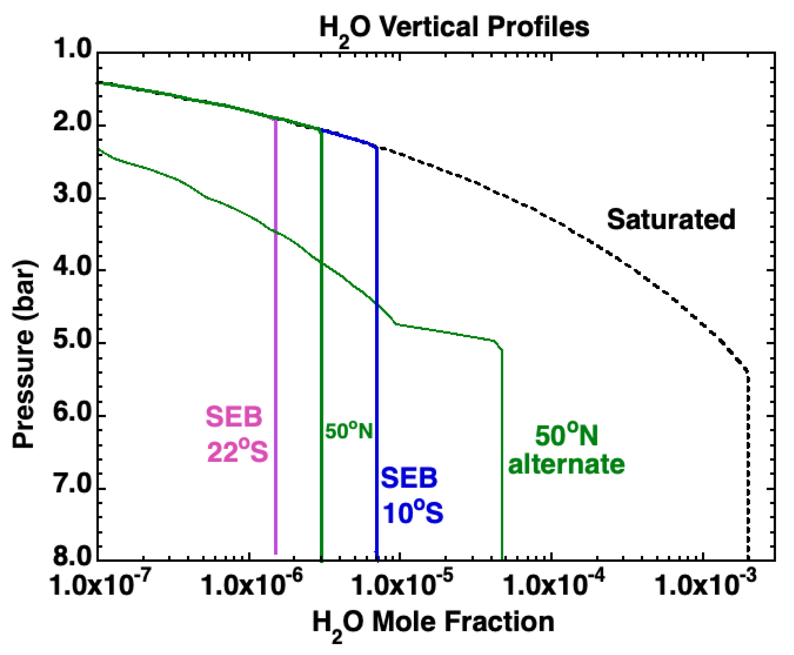
We calculated models for three abundances of HO at 50N, as shown in Figure 13. The best fit, 3.0 ± 0.3 ppm for p > 2.5 bar, made use of a strong HO absorption feature at 2016.8 cm in addition to the target line pair near 2018 and 2019 cm. We also plot the retrieved mole fractions of HO as a function of latitude between 70S and 66N (Figure 14). The vertical profile of HO is assumed to be constant for p > 2.5 bar and following a saturated profile at lower pressures. The retrieved abundances for three latitudes and their vertical profiles are shown in Figure 15. In regions without water clouds, gaseous HO ranges from 1.5 ppm at 22S to 7 ppm at 10S.
The retrieved HO abundance increases to 14 ppm in regions with water clouds, such as in the SEB Outbreak region at 13S. However, as discussed earlier, HO mole fractions retrieved for latitudes with water clouds are not valid in the 4–7 bar pressure range if water clouds are accompanied by ∼1000 ppm gaseous HO below their cloud tops. Information derived from our targeted HO line pair would pertain to the 3 bar level, rather than to the pressures shown in Figure 14. The retrieved values in the belts are significantly sub-saturated, as shown by the dashed line in Figure 15. Sub-saturation is expected in relatively cloud-free regions, such as the NEB and SEB, but not in regions with water clouds.
There is some degeneracy in our sensitivities to the vertical profile and the deep concentration of water vapor. Green lines in Figure 15 show two acceptable fits to the 50N spectrum: our preferred distribution with a constant value of 3 ppm, and one with 47 ppm HO in the 5–8 bar region, dropping off at pressures <5 bar (maintaining roughly 1% relative humidity at the lower pressures). Both profiles have the same HO mole fraction at 4 bar. The alternate profile—similar to the one used in our previous study of the SEB [9]—is consistent with the Galileo Probe Mass Spectrometer (GPMS) concentration of 40 ± 13 ppm [23].
However, it is important to note that the GPMS was not sensitive to HO concentration at bar, while our spectroscopic retrieval is not sensitive to HO concentration at bar (and limited to even shallower pressures when opaque clouds are present). Although the alternate profile with 47 ppm HO at bar provided an acceptable fit to the spectral data at 50N, the fit was poorer at other latitudes. Our analysis favors lower concentrations in the 5 to 8 bar region. New 5 µm spectra of Jupiter from the James Webb Space Telescope using weak HO absorption lines that are blocked by the Earth’s atmosphere may allow us to distinguish between these two vertical profiles.
The low HO concentrations in the 5 to 8 bar region are consistent with a widespread deep gradient in water. The GPMS measured increasing HO from 11 bar to its deepest measurement at 20 bar. Although this deep gradient has been explained in terms of local meteorology in 5 µm Hot Spots, e.g., [26,27], the widespread deep ammonia gradient from Juno and VLA microwave observations [24,28,29] suggests dynamical processes that may control the water vapor profile as well. Widespread gradients are needed for our depleted HO values to increase between 8 bar to the higher values measured by Galileo and implied by the existence of condensation clouds at pressures greater than 3 bar.
3.3. Storms in the South Equatorial Belt
A convective superstorm known as an “SEB outbreak” erupted in Jupiter’s South Equatorial Belt (SEB) in late 2016. Compositional and aerosol anomalies in the storm and nearby regions were characterized using observations in January 2017 at multiple wavelengths from ALMA, VLA, HST, VLT, Subaru, Gemini, and Keck [5]. The Keck data included NIRSPEC observations at 5 µm obtained on 11 January 2017. de Pater et al. [5] reported a lower limit to the NH mole fraction of 300 ppm in a region called the “East Disturbance” at 13S. This value was reported as a lower limit rather than an abundance in the core of the storm. This is because the NIRSPEC slit included regions adjacent to the storm that contributed more 5 µm flux than the storm itself.
Our February 2017 spectroscopic data characterize the active phase of the SEB outbreak, which continued through March 2017 (with minor residual activity persisting through summer of 2017, see Rogers 2018, report no. 17). The NIRSPEC spectra described in Section 3.1 cut through the SEB storm region when the slit was placed on the central meridian. Atmospheric properties derived from the spectral analysis are graphically summarized in Figure 16, overlaid on a Section of the map from Figure 1. The same atmospheric properties are also plotted in Figure 17 and Figure 18.
In Figure 17, we show an enlargement of Figure 5 indicating the pressure level of deep clouds over the same latitude range as Figure 16 (between 30S and the equator). The CHD EW retrieval indicates an opaque water cloud near 5.5 bar at 13S (green line), while the low continuum radiance (black line) indicates upper-level cloud opacity consistent with the HST maps (the white mushroom cap in Figure 16). As discussed earlier, the pressure of the water cloud at 13S is likely to be overestimated.
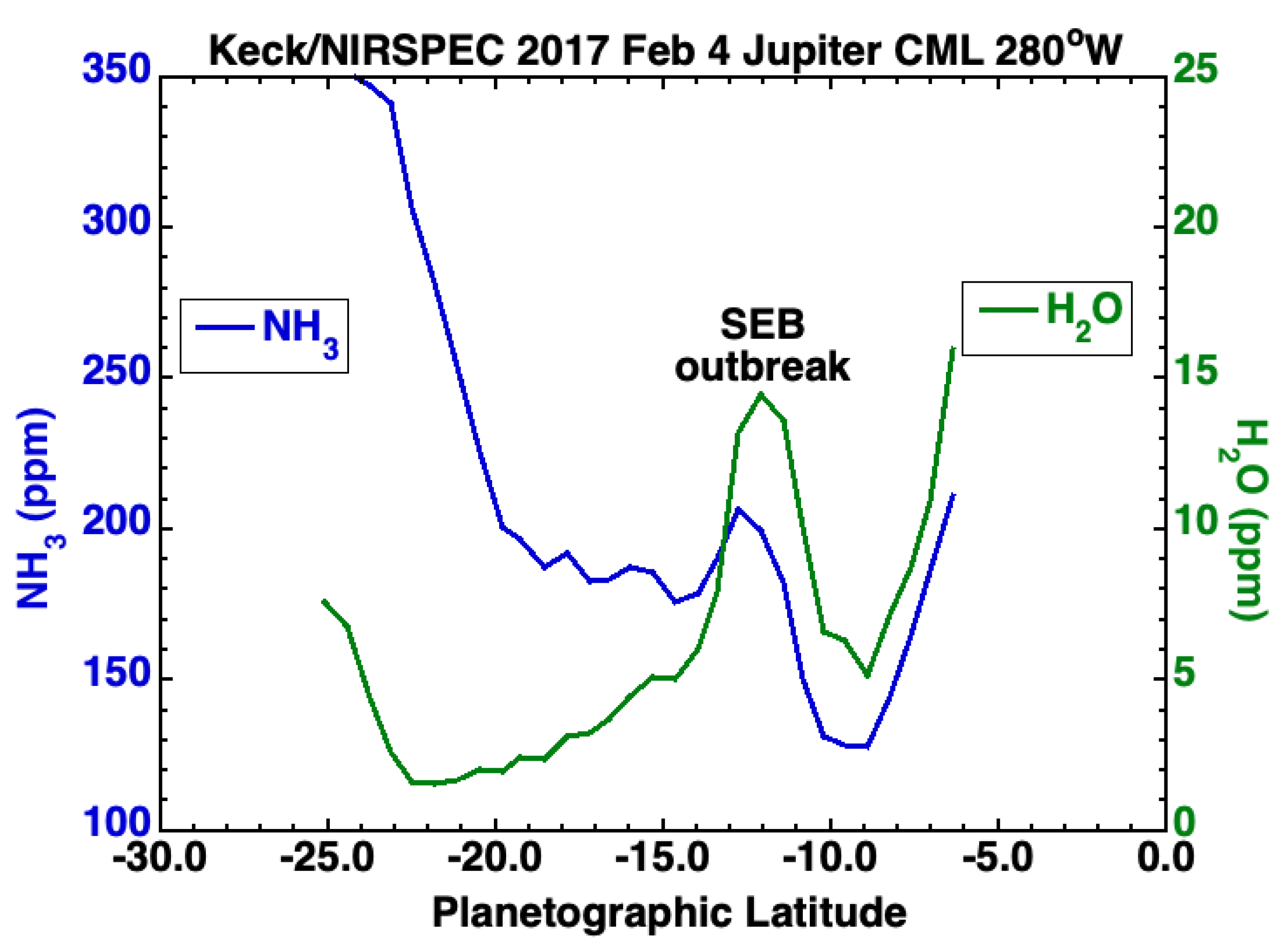
Figure 18 shows the derived mole fractions of NH and HO obtained using the EWs of absorption features at 4.97 µm. The mole fraction of NH has a local maximum (whose value is likely underestimated) at 13S, exactly at the location of a water cloud derived from CHD spectra at 4.66 µm, shown in Figure 11. The derived HO mole fraction also has a maximum here, and its value is almost certainly underestimated in this retrieval. These results are consistent with a rising parcel of air transporting both gases from deeper levels, in agreement with the scenario suggested based upon the January 2017 data [5].
3.4. Cloud Variation in the North Equatorial Belt
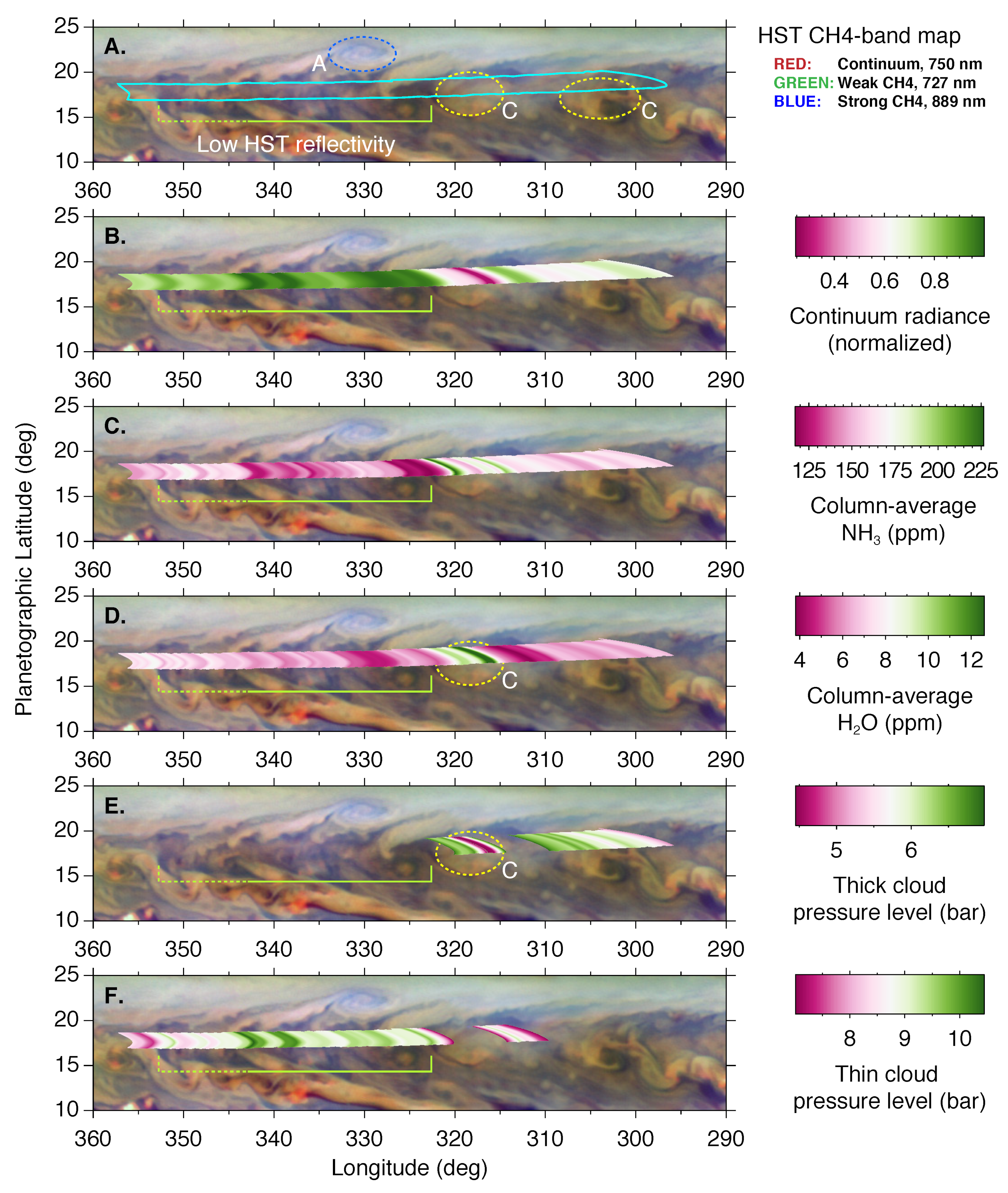
In addition to our study of the latitudinal variation of Jupiter’s deep clouds, we investigated the North Equatorial Belt, retrieving gas and aerosol properties at two locations centered at 18N (Figure 19) and at 8N (Figure 20). Highlights at 18N include the presence of thick water clouds and locally-enhanced water vapor over the optically bright region at 320W in the HST image, which is likely a cyclonic vortex to the west of a vortex series associated with mesoscale waves [31,32]. There is minimal cloud opacity in an optically dark area covering the western half of the slit, which also has low NH concentration but no prominent anomaly in HO concentration.
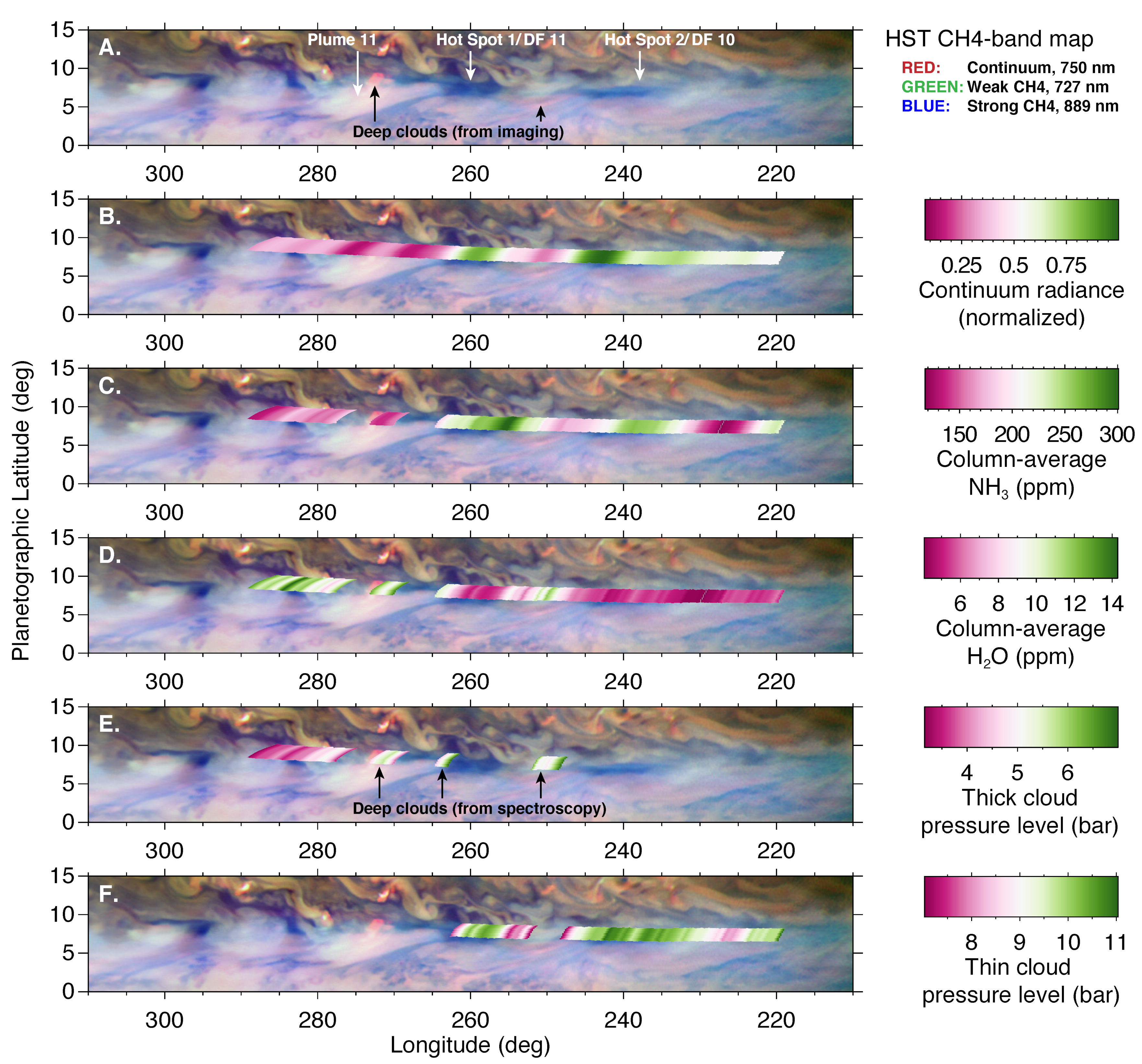
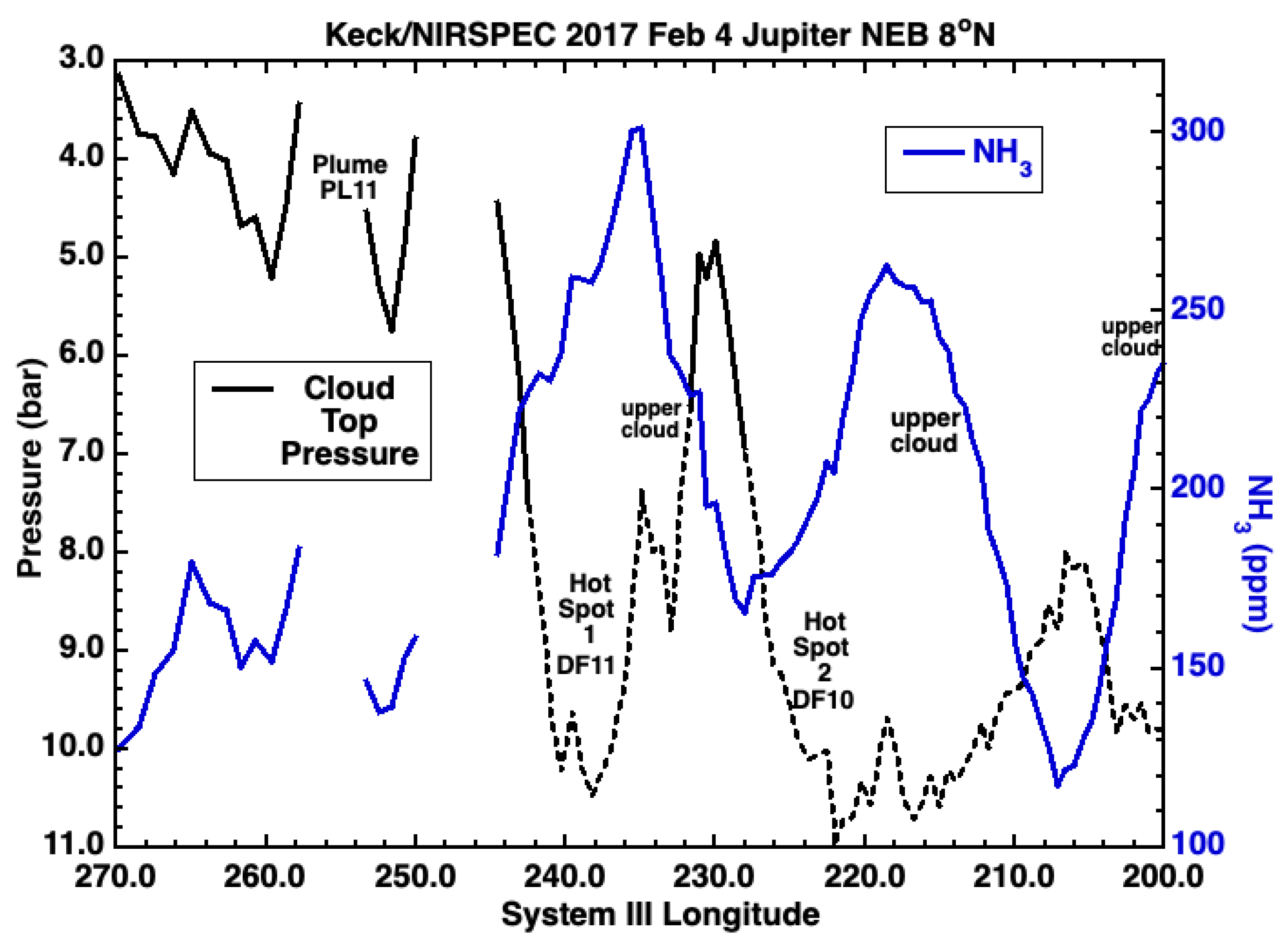
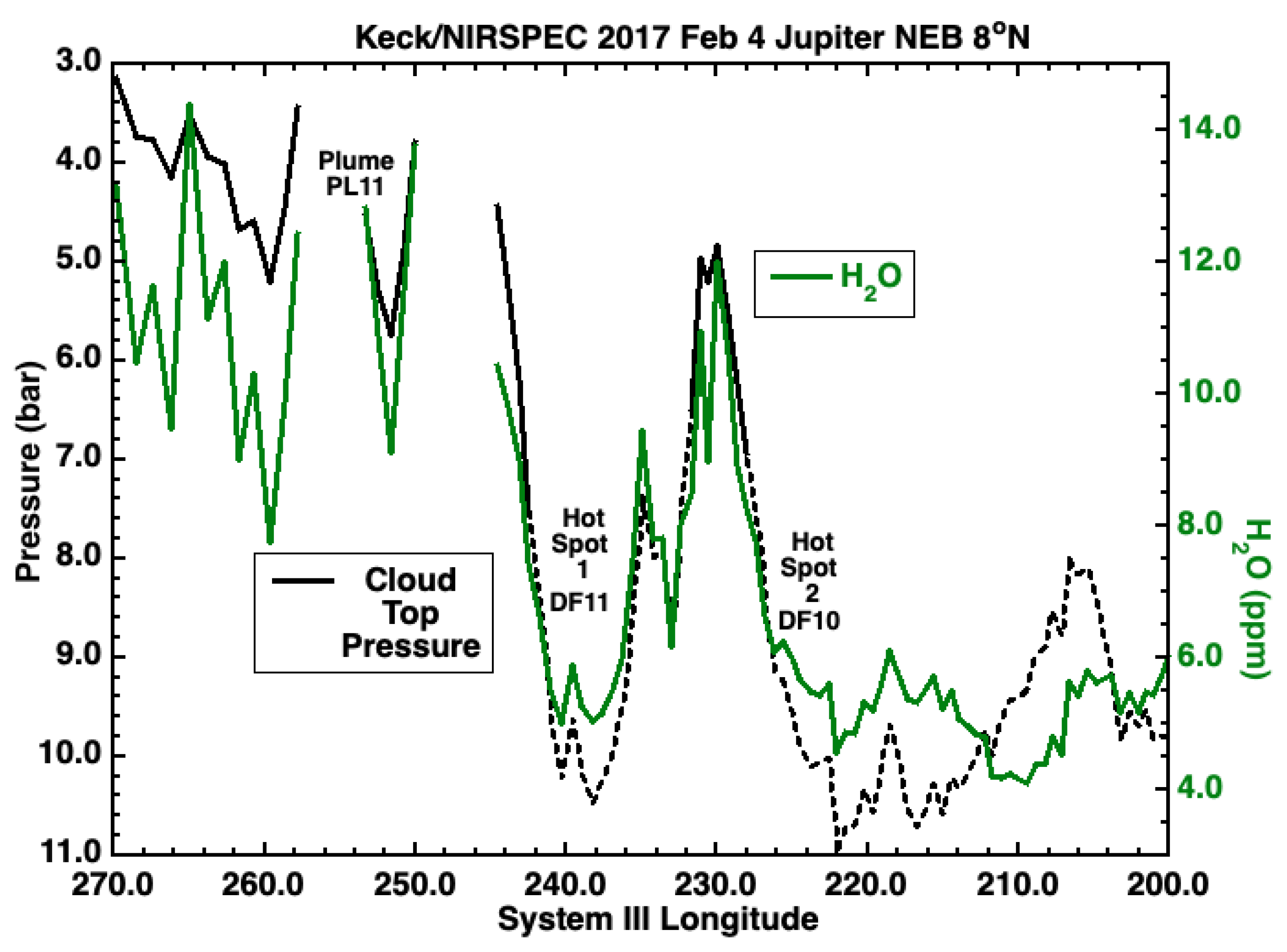
The NEB at 8N exhibits an amazing amount of structure. The eastern half of the slit samples two Hot Spots, which appear deep blue in the HST image because upper tropospheric hazes—which appear blue in CH-band composites—are not depleted in Hot Spots. The western portion includes deep water clouds, unobscured by overlying upper clouds, that appear red in the CH-band composite. This latitude is close to that of the entry site of the Galileo Probe, which relayed in situ data some 21 years earlier.
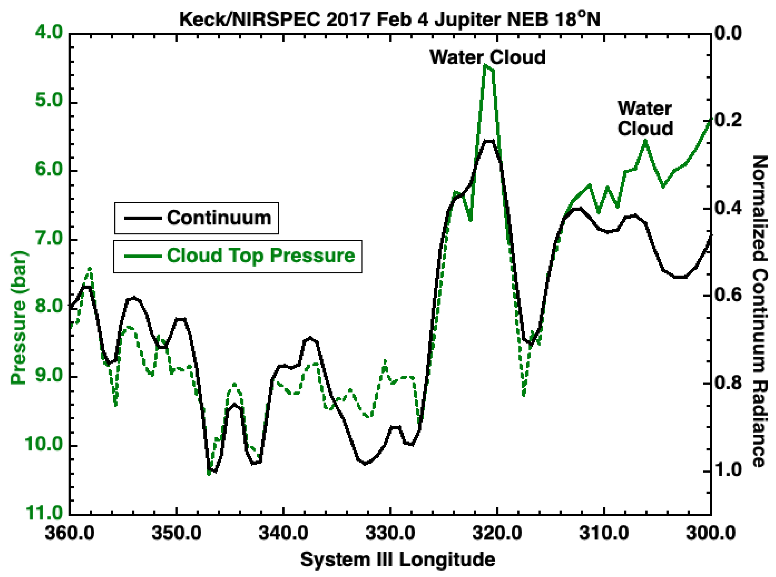
In Figure 21, we show the continuum radiance and derived cloud-top pressure in the NEB at 18N between 300W and 360W longitude. Low values of CHD EW indicate water clouds at 306W and 321W. There are no opaque clouds between 325W and 360W. However, there is a strong correlation between continuum radiance and apparent cloud-top pressure. We measured minute changes in CHD EW at the 1% level. This is not due to upper clouds because upper clouds do not affect CHD EW. This is either due to deep clouds or due to variations in gaseous HO for p > 5 bar. If this is a result of cloud opacity, then we interpret this variation in EW to the presence of optically thin water clouds between 4 and 7 bar rather than opaque clouds between 8 and 10 bar.
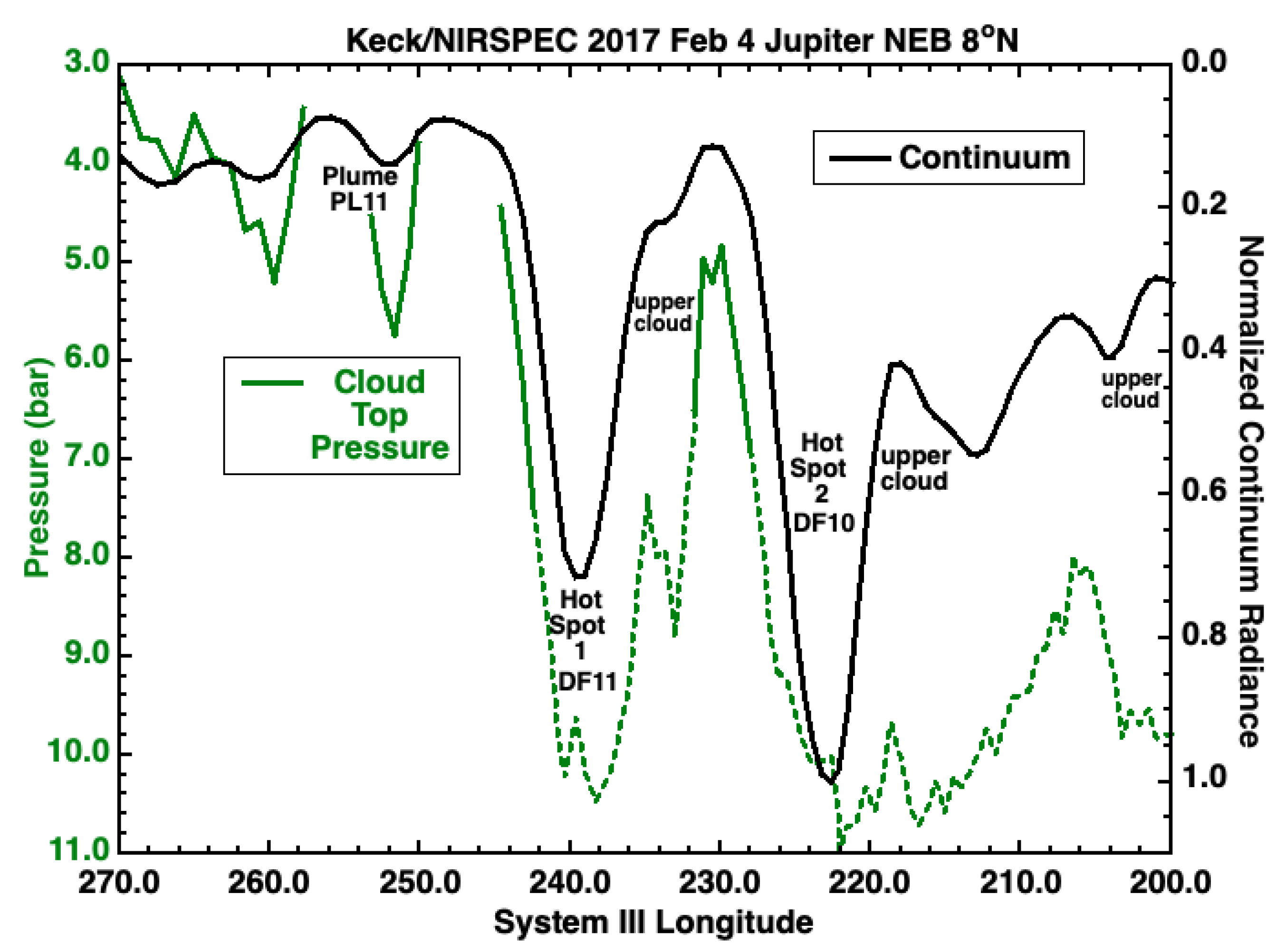
In Figure 22, we show a heterogeneous portion of the NEB at 8N near the latitude of the Galileo Probe entry site. There is evidence for Hot Spots, water clouds, and upper clouds at different longitudes between 200W and 270W. From imaging studies Hot Spots with cloudy regions in between them are expected; however, this is the first study using 5 µm data alone to distinguish between water clouds and upper (NH or NHSH) clouds in this region.
![Remotesensing 14 04567 g019]()
![Remotesensing 14 04567 g020]()
![Remotesensing 14 04567 g021]()
Figure 19.
The retrieved properties near 18N in the North Equatorial Belt, compared with HST imaging. Panel (A) shows the three filters used by HST, the location of the slit, and the presence of three vortices on Jupiter. Features marked A and C resemble anticyclonic and cyclonic vortices associated with mesoscale waves in studies of visible light and 5 µm imaging data in the 2017 timeframe [31,32]. The possible cyclone near 320W covered the full width of the NIRSPEC slit, and is characterized by relatively high amounts of water vapor and deep cloud opacity (panels (D,E)). The western portion of the slit footprint covers a region of low cloud reflectivity in the HST imaging data, marked with a green bracket. This region was associated with high continuum radiance (panel (B)), the lowest NH concentration (panel (C)), and very low deep-cloud opacity (panels (E,F)). The water abundance in the low-reflectivity region did not appear anomalously low (panel (D)). The longitudes of the retrieved properties shown here were adjusted using the zonal wind profile [7] to match positions in the HST maps acquired about 3 days before the Keck spectra, while the longitudes of the retrieved properties in Figure 21, Figure 23 and Figure 24 differ because they are shown at the time of observation.

Figure 20.
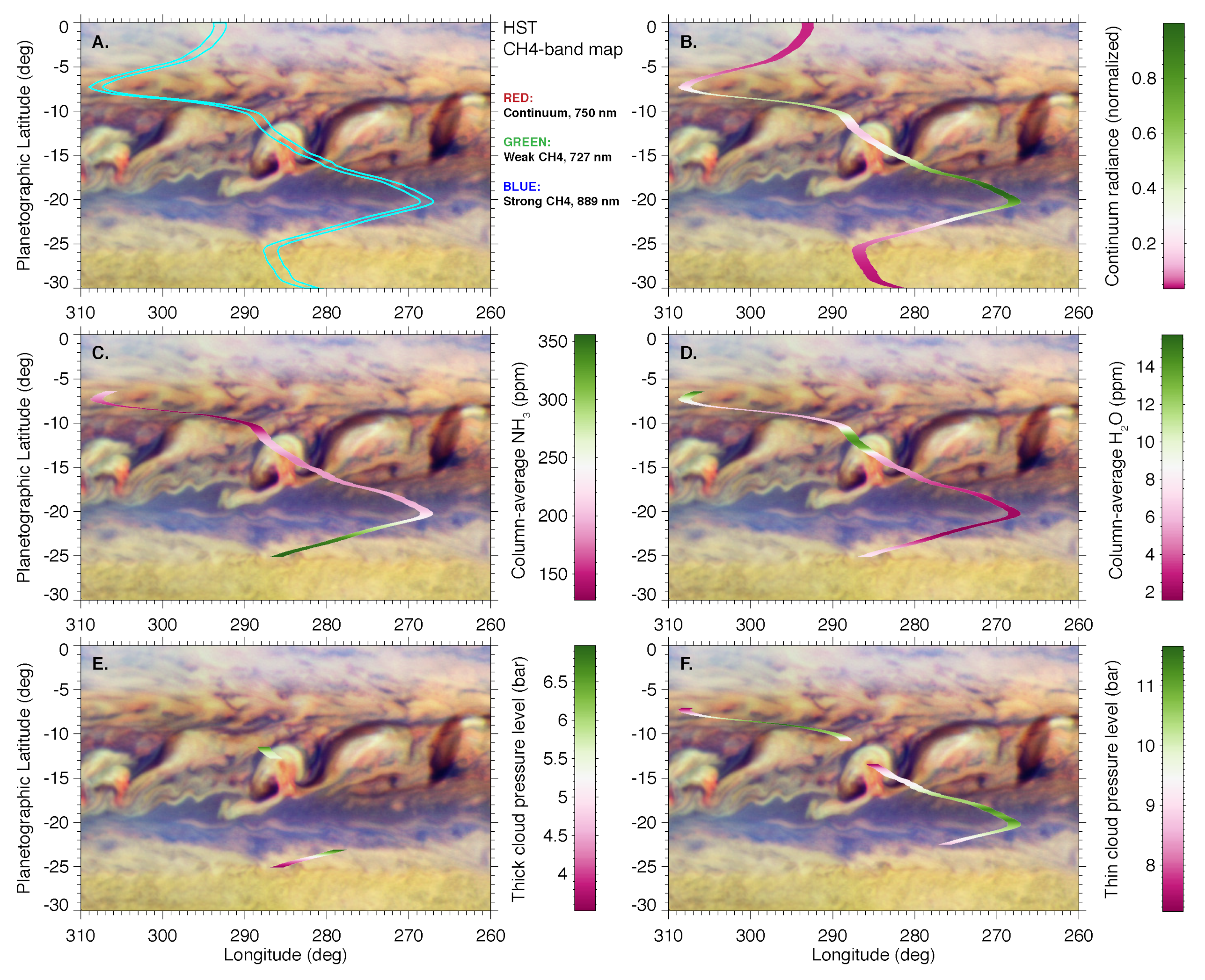
The retrieved properties near 8N in the North Equatorial Belt. Two Hot Spots (marked in panel (A)), which were also described in Fletcher et al. [33], are generally associated with very low deep-cloud opacity and low volatile concentrations, although the distribution of HO and NH vapor within the Hot Spots differs. Panels (B–F) denote the same parameters as in Figure 19. There is a strong correspondence between the locations of deep clouds identified in imaging data by their high continuum/727-nm ratios (red color in panel (A)), and deep clouds identified in the spectral data by their narrow CHD EW (retrieved moderate to low thick cloud pressure levels in panel (E)). The longitudes of the retrieved properties shown here were adjusted using the zonal wind profile [7] to match the positions in the HST maps acquired about 3 days before the Keck spectra, while the longitudes of retrieved properties in Figure 22, Figure 25, and Figure 26 differ because they are shown at the time of observation.
Figure 20.
The retrieved properties near 8N in the North Equatorial Belt. Two Hot Spots (marked in panel (A)), which were also described in Fletcher et al. [33], are generally associated with very low deep-cloud opacity and low volatile concentrations, although the distribution of HO and NH vapor within the Hot Spots differs. Panels (B–F) denote the same parameters as in Figure 19. There is a strong correspondence between the locations of deep clouds identified in imaging data by their high continuum/727-nm ratios (red color in panel (A)), and deep clouds identified in the spectral data by their narrow CHD EW (retrieved moderate to low thick cloud pressure levels in panel (E)). The longitudes of the retrieved properties shown here were adjusted using the zonal wind profile [7] to match the positions in the HST maps acquired about 3 days before the Keck spectra, while the longitudes of retrieved properties in Figure 22, Figure 25, and Figure 26 differ because they are shown at the time of observation.

Figure 21.
The pressure of the lower boundary derived from CHD (green curve) is shown as a function of longitude in the NEB at 18N. The continuum radiance is shown in black. Regions with p > 7 bar (dashed green) do not have opaque clouds; however, they may have optically thin water clouds. Longitudes where p < 7 bar (e.g., 306W and 321W) are interpreted as having opaque water clouds. See Figure 19 for a comparison with HST images.

There are two Hot Spots at 222and 238, denoted as Hot Spot 2 and Hot Spot 1. They coincide with Dark Formations DF10 and DF11, which were studied a few weeks later at longer wavelengths by Fletcher et al. [33]. The combination of these two datasets provides strong constraints on the nature of Hot Spots, as discussed in Section 4.4. Both regions have high continuum radiances and high CHD EWs. Immediately to their east, there are regions with upper clouds between 214 and 220 and 233–236. In addition, there are upper clouds near 200.
Figure 22 also shows opaque water clouds at 230W, and between 242 and 270W. Note that there is a red region at 8N and 272W in the HST methane-band image displayed in the lower right of Figure 1 and in Figure 20. Red indicates more reflected sunlight in a continuum channel (750 nm) between methane bands than at wavelengths where methane absorbs strongly (727 and 889 nm). This provides evidence for deep clouds, although it is difficult to quantify their exact pressure. Zonal winds at 8N will advect the cloud in the HST image from 272W to ∼252W over the 3 day interval between the HST and Keck observations.
This places this feature at a location with low CHD EW, which supports the interpretation that the red feature in the HST image is, in fact, a water cloud. This is close to the location of plume PL11 observed in [33]. There is additional evidence for a correlation between red features and areas with low CHD EW in the SEB outbreak region, as described in Section 3.3, that helps to validate the use of HST methane-band images to detect water clouds. Clearly, this latitude is heterogeneous; thus, caution must be used to apply the results of the Galileo Probe to other regions on Jupiter, even in the same latitude band.
![Remotesensing 14 04567 g022]()
Figure 22.
The pressure of the lower boundary derived from CHD (green curve) is shown as a function of longitude in the NEB at 8N. The continuum radiance is shown in black. Longitudes where p < 7 bar (e.g., 244W to 270W) are interpreted as having opaque water clouds. Upper clouds are present at longitudes with high CHD EW (dashed green) and low continuum radiance (200W, 217W, and 233W). Hot Spots 1 and 2 are the same features as Dark Formation DF11 and DF10, studied in detail in [33]. The cloudy region near 252W corresponds to plume PL11 in the same study. This is also near the area where HST CH-band imaging shows the presence of deep clouds (see Figure 1 and Figure 20).

3.5. Variations in the Ammonia and Water Abundances within the North Equatorial Belt
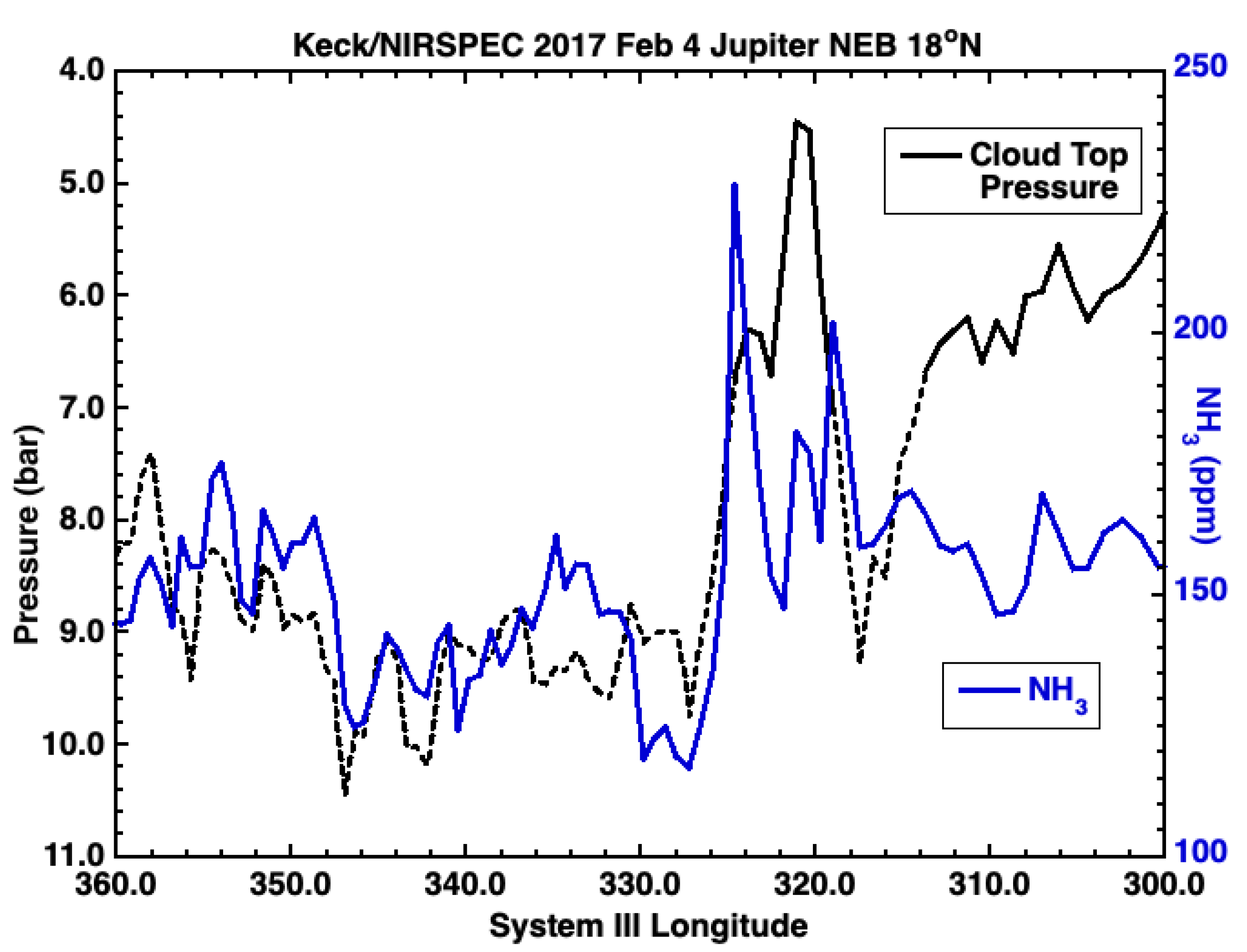
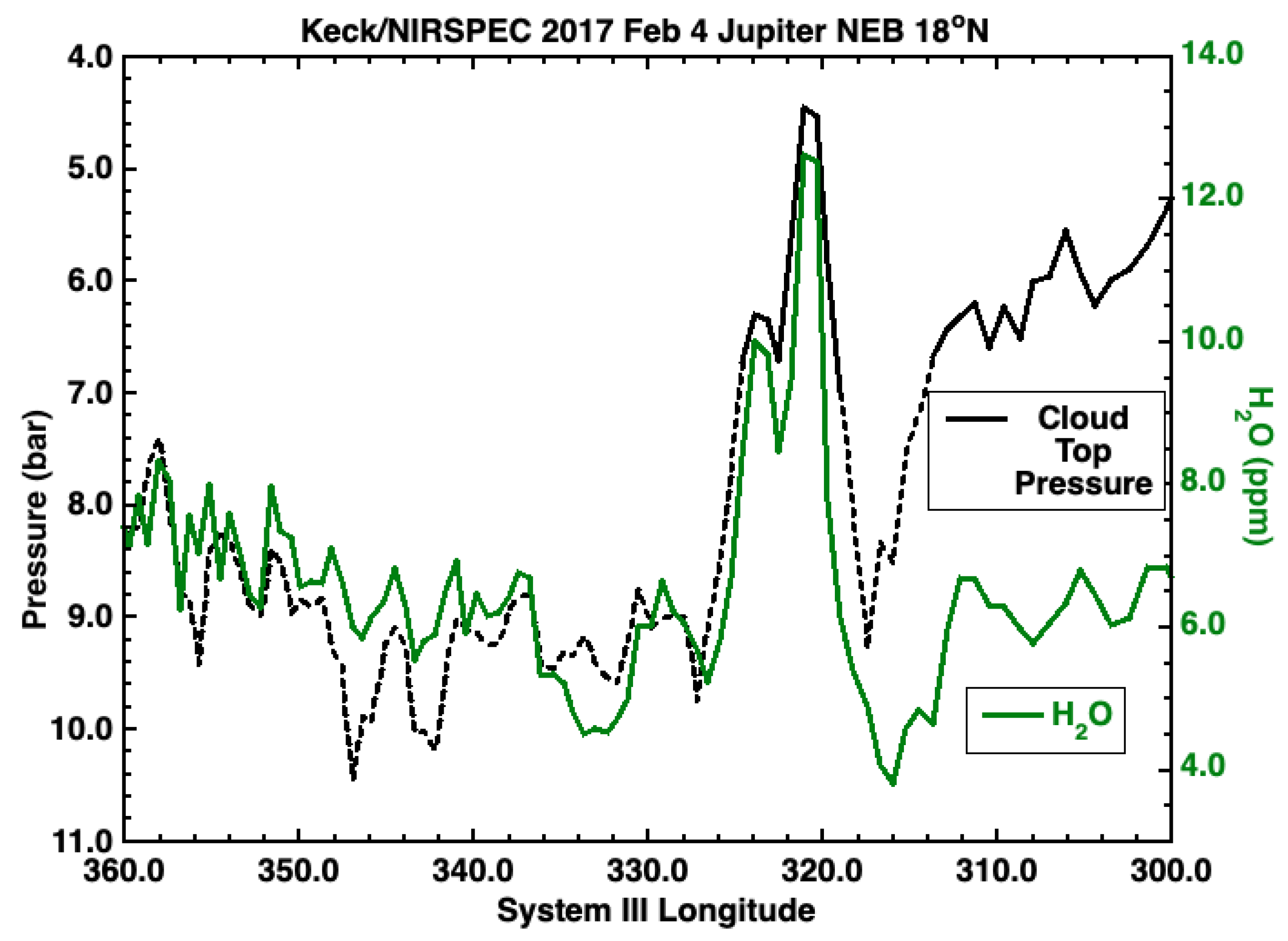
Using the cloud-top pressures described in the previous section, we measured the variation with longitude of the two principal volatiles on Jupiter, NH and HO, at 18N in the North Equatorial Belt. In Figure 23 we show that NH is in the 120–150 ppm range near 6 bar in regions lacking opaque water clouds. Its abundance rises to around 200 ppm between 318 and 326W where there is higher cloud opacity. Similarly, in Figure 24 we indicate that the mole fraction of gaseous HO is in the 4–8 ppm range near 6 bar and increases significantly at the cloudiest longitude near 321W. This same longitude does not exhibit a maximum in NH; therefore, it is not analogous to the outbreak region in the SEB.
The NEB at 8N is an interesting and complicated region on Jupiter. The most surprising feature in Figure 25 is the lack of correlation between NH and the two Hot Spots at 222W and 238W (Dark Formations DF10 and DF11 in [33]). Derived NH mole fractions in these Hot Spots are in the 200–250 ppm range; however, they are neither minima nor maxima. Instead, there is a wave-like oscillation between 200 and 250W with a factor of 2 variation in NH mole fraction ranging from 120 to 250 ppm. This is not an artifact of the derived cloud structure, as it is seen in the measurements of NH equivalent widths. The maxima occur near longitudes where upper clouds were inferred, as shown in Figure 22. Plume PL11 occurs near a region with significant reflected sunlight; thus, NH and HO values are not available here.
In Figure 26, the derived HO, mole fractions range from 3 to 14 ppm across this longitude range. Gaseous HO is strongly correlated with cloud-top pressure. Here, again, Hot Spots do not stand out when compared with adjacent regions with low cloud opacity. Hot Spot 1 (DF11) is evident as it is surrounded by cloudy regions; however, Hot Spot 2 (DF10) has the same HO abundance (5 ppm) as adjacent longitudes between 200 and 220W. There is no evidence for any periodic oscillation in HO mole fraction over the 200 to 250W range of longitudes where NH variation occurs.
![Remotesensing 14 04567 g023]()
![Remotesensing 14 04567 g024]()
![Remotesensing 14 04567 g025]()
![Remotesensing 14 04567 g026]()
Figure 23.
The NH mole fraction in ppm (blue curve) is shown for the NEB at 18N as a function of longitude between 300W and 360W. The pressure of the lower boundary derived from CHD is shown in black. Most longitudes have NH in the 120–200 ppm range. See Figure 19 panel C for an overlay onto the HST image.

Figure 24.
The HO mole fraction in ppm (green curve) is shown for the NEB at 18N as a function of longitude between 300W and 360W. The pressure of the lower boundary derived from CHD is shown in black. Most longitudes have HO in the 4–8 ppm range. See Figure 19 panel D for an overlay onto the HST image.

Figure 25.
The NH mole fraction in ppm (blue curve) is shown for the NEB at 8N as a function of longitude between 200W and 270W. The pressure of the lower boundary derived from CHD is shown in black. The Hot Spots do not exhibit minima (or maxima) in NH. Hot Spots 1 and 2 are the same features as DF11 and DF10 in [33]. The ammonia mole fraction appears to be correlated with the presence of upper clouds, as inferred by high CHD equivalent widths and low continuum radiances. See Figure 20 panel C for an overlay onto the HST image.

Figure 26.
The HO mole fraction in ppm (green curve) is shown for the NEB at 8N as a function of longitude between 200W and 270W. The pressure of the lower boundary derived from CHD is shown in black. Hot Spots have less HO than regions inferred from CHD to have water clouds; however, they do not stand out when compared with adjacent regions that also lack water clouds. Hot Spots 1 and 2 are the same as DF11 and DF10 in [33]. See Figure 20 panel D for an overlay onto the HST image.

4. Discussion
This paper describes a technique to determine water cloud heights using the integrated absorption, or equivalent width, of CHD. We demonstrated with a set of spectra from characteristic spatial regions that variation in the water cloud height manifests as a variation in the equivalent width of CHD. We applied this technique to Jupiter’s Central Meridian, to the NEB at 18N, and to the latitude of the Galileo Probe entry site near 8N. Using the derived pressure of the deep cloud tops as an opaque lower boundary, we obtained column-averaged mole fractions of NH and HO. Knowledge of the spatial variation and pressure level of water clouds, combined with abundances of condensing gases, such as NH and HO opens up a new field of study of Jovian dynamics between 1 and 10 bar. In addition, our observations can place the Galileo Probe data into regional context, with the caveat that these observations are separated by 21 years in time.
4.1. Ammonia Abundance
A comparison of our retrieved NH abundances with those reported by Grassi et al. [34] based upon Juno/JIRAM data shows good agreement at 10N in the NEB, where both studies find 100 ppm NH. Elsewhere, JIRAM values are 300–350 ppm, somewhat higher than our values of 200–250 ppm. Grassi et al. [34] focused on infrared-bright spectra only (defined as <3% reflected sunlight); however, our analysis using resolved spectral lines allowed us to set a less restrictive limit. We include infrared-dark regions with significant upper cloud opacity (reflected sunlight < 10%).
We found that the regions with high upper cloud opacity also had higher ammonia concentration (in the regime of 3–10% reflected sunlight where we were able to retrieve ammonia; see Figure 4 and Figure 11). The difference in spectra selected for analysis thus does not explain the difference in retrieved concentrations, because the darker spectra included in our study should bias the results toward higher concentrations, while our overall concentrations were instead lower than in Grassi et al. [34].
Our retrieved NH mole fractions are approximately 100 ppm smaller than Giles et al. [35] who measured a set of absorption features of NH at 5.156, 5.157 and 5.184 µm (1939.5, 1939, and 1929 cm) sensitive to the 1.6–3.3 bar level on Jupiter. They observed Jupiter in November 2012 using the CRIRES spectrometer on the Very Large Telescope in Chile at a resolving power of 96,000, or 0.02 cm at 2000 cm. These authors reported values of NH ranging from 100 to 400 ppm with a vertical profile increasing between 1.6 and 3.3 bar.
In the NEB at 8N, their values for NH increased from 60 ppm at 1.6 bar to 300 ppm at 3.3 bar. They also retrieved much larger values of 700 ppm at 13S and 1500 ppm in the EZ at 5N. This latter value was reduced to 500 ppm by introducing an opaque cloud at 5 bar. Although we did not model the EZ, this illustrates the extreme sensitivity to the pressure of the lower boundary. The apparent high value at 13S may also be explained if water clouds were present at this latitude in 2012 when their spectra were acquired. They did not model reflected sunlight in their analysis.
Our retrieved NH mole fractions are in excellent agreement with those of Blain et al. [36] who reported values ranging from 60 to 160 ppm at 10N to 300 ppm at 20N and 30S using a pair of strong absorption features at 5.156 and 5.157 µm (1939.5 and 1939 cm) sensitive to the 2 bar level. Note that this is the same line pair as observed in [35]. Reflected sunlight was not taken into account in the zones.
Blain et al. [36] retrieved NH at multiple longitudes at each latitude whereas Giles et al. [35] retrieved gas abundances from one north–south slit position. The data in [36] were acquired in January 2016 with the TEXES spectrometer on the Infrared Telescope Facility in Hawaii at a spectral resolution of 0.15 cm, similar to that of our Keck data. These authors retrieved a vertical gradient of ammonia below the NH condensation level, with 500 ppm NH at 3 bar falling off to 100 ppm at 1 bar in Jupiter’s zones. Sub-cloud ammonia gradients were found in observations from the Galileo Probe, the VLA, and Juno.
We can compare our retrieved NH values with the abundances derived from microwave data acquired using the Very Large Array (VLA) (Figure 5, Figure 11 and Figure 12 of de Pater et al. [24]). At 10N, the authors retrieved an NH abundance of 175 ppm between 20 and 1.5 bar, decreasing to 20 ppm from 1.5 to 0.7 bar, and dropping below 0.1 ppm at 0.3 bar. Given the large variability of NH with longitude in the NEB, this represents good agreement between our infrared data and the microwave data in de Pater et al. [24]. The NH abundance at 6 bar retrieved from VLA data ranged from 180 to 340 ppm as a function of latitude (excluding the EZ), in excellent agreement with results from this study.
Our 5 µm NH abundances are in agreement with Juno MWR values at 6 bar ranging from 100 ppm in the NEB to 250 ppm in the SEB as reported by Li et al. [28]. These authors also reported a decrease in NH from 250 ppm at 2 bar to a minimum of 200 ppm at 7 bar at latitudes outside of the EZ. The ammonia mole fraction may be strongly depleted at 6 bar with respect to measurements at deeper levels from the Galileo Probe. Probe radio signal attenuation gave a maximum concentration of 755 ± 100 ppm NH at 9.7 bar in an initial study [37], updated to 835 ± 60 ppm after additional laboratory measurements of the ammonia opacity under Jovian conditions [38].
Wong et al. [23] reported a mole fraction of 566 ± 216 ppm NH between 9 and 12 bar as measured by the mass spectrometer on the Probe. Both signal attenuation and mass spectrometry pertain to the probe entry site near 7N. Different vertical profiles, with NH either constant with pressure or increasing only by 40% between 6 and 20 bar, would contradict the Probe results but would be consistent with Juno MWR data. Li et al. [39] reported 351 ± 21 ppm NH at the 20 bar level in the EZ. Li et al. [28] reported similar values at all latitudes for p > 40 bar.
4.2. Water Abundance
A comparison of retrieved water vapor from JIRAM data reported by Grassi et al. [34] shows that we obtain the same extrema in HO: 22S is the latitude with the minimum abundance and 10S exhibits the maximum value. Grassi et al. [34] express HO in terms of relative humidity ranging from 0.1 to 10%. These authors did not specify a pressure level; thus, comparisons between humidity and mole fraction will not be exact. We will assume that both datasets contain information at the 4 bar level where the saturated mole fraction of HO is 360 ppm using the Galileo Probe temperature profile [6]. Our results of 1–15 ppm HO mole fraction correspond to relative humidities between 0.3 and 4%, in good agreement with [34].
Our data do not directly constrain the deep HO abundance because gaseous HO cannot be retrieved within or below an opaque water cloud. Our data are also insensitive to composition at the ∼20 bar level where Li et al. [39] find 1–5 times solar O/H. Our measurements in regions with low cloud opacity (9 ppm near 6.5 bar) correspond to ∼1% protosolar O/H (assuming a hydrogen mixing ratio of 0.86 from the Galileo Probe [16,40] and protosolar abundances from Asplund et al. [41]). We can derive indirect constraints on O/H from our analysis, because the cloud levels retrieved from CHD EW serve as lower limits to the pressure of the cloud base. This indirect constraint is explored in more detail in Wong et al. [42].
Our retrieved HO abundances are in good agreement with Giles et al. [43] who analyzed Cassini VIMS spectra of the night side of Jupiter at 5 µm acquired during its flyby in January 2001. Both VIMS and JIRAM have similar spectral resolving power of 270, or 7 cm at 2000 cm. These authors found a maximum of 3% humidity near 10S and a minimum of 0.2% near 20S. However, Giles et al. [43] assumed a deep solar abundance below the water condensation level (with their stated relative humidities applying to altitudes above the condensation level) so the average column abundances implied by their results are actually higher than the values from our retrievals.
An extreme sub-saturation of HO is seen in Jupiter’s belts and Hot Spots. This may be explained by the same theory that explains the global depletion of ammonia gas in the upper atmosphere. Building upon a suggestion by Ingersoll et al. [44], Showman and de Pater [45] postulated a double-stacked circulation pattern, with air descending in belts at altitudes above the water cloud, and rising upwards deeper in the atmosphere.
The water cloud layer acts as a barrier against convection from below; however, occasionally storms do rise up through this layer. Such thunderstorms may dry out Jupiter’s atmosphere through rainout of NH ice, or NH trapped in water or in NHSH particles. A similar circulation was suggested by Fletcher et al. [46] to explain Juno/MWR data, and Duer et al. [47] developed a numerical code to model the variations in ammonia with latitude and altitude. The necessary large size of the particles to make this process work was solved by Guillot et al. [48], who showed that water ice could be lofted up to almost the 1 bar level, where mixed-phase NH and HO condensates and hydrates can allow aerosol particles to grow to cm-sized hail, referred to as “mushballs”. Such large particles can fall down to high pressure levels ([45,48]). This process may also cause water to be extremely sub-saturated in Jupiter’s upper troposphere [49,50].
The apparent sub-saturation of gaseous HO in regions with water clouds implied by Figure 14, Figure 18, Figure 24 and Figure 26 is almost certainly not real. As discussed earlier, water clouds are likely to be accompanied by large values (∼1000 ppm) of HO below their cloud tops, rather than the 4-ppm value assumed in our retrievals. Our technique is sensitive to spatial variation in the HO column abundance but it is affected by variation in the depth of the column probed when deep clouds are present.
Even in the absence of clouds, we do not find HO volume mixing ratios as high as the 420 ppm detected by the Galileo Probe around 20 bar [23], let alone the 2500 ppm retrieved from analysis of equatorial Juno MWR data [39]. Thus, our measurements strongly support the existence of a deep gradient in the water-vapor concentration that extends well below the 8 to 10 bar lower limit of our sensitivity (Figure 8).
4.3. Clouds
Grassi et al. [34] modeled JIRAM spectra of Jupiter with a spectrally flat cloud extending between 0.7 and 1.3 bar, presumably an NH cloud. Giles et al. [35] adopted a similar cloud model. Grassi et al. [34] tested the introduction of a deep cloud at 5 bar as proposed in [9]; however, they found no improvement in the fit to the JIRAM data and, thus, they did not use a deep cloud in their study. The difference between the current study and that of Grassi et al. [34] may be related to spectral resolution, the depth probed in Jupiter’s atmosphere, and signal to noise.
The JIRAM spectral resolution of 7 cm reveals only the strongest absorption features of HO and NH which primarily sound levels less than 5 bar. In contrast, Giles et al. [35], using higher spectral resolution data, found that their retrievals were sensitive to clouds at 5 bar. The JIRAM study excluded low-flux regions where water cloud opacity may be important. Our study excluded some of the same regions due to high values of reflected sunlight; however, we also found evidence for water clouds in the SEB Outbreak region and in other locations.
Our assumption of an opaque lower boundary due solely to cloud opacity is certainly an oversimplification. Additional modeling incorporating multiple scattering of thermal radiation to treat clouds with a finite vertical extent, and including HO gas opacity below the cloud tops may be needed; however, this is beyond the scope of the current study. One of the key results of this study is the ability to distinguish upper clouds from deep clouds in areas which have low 5 µm continuum brightness but large values of CHD equivalent width. This technique will enable studies that seek to determine which cloud layer(s) are responsible for time-varying changes in the latitudinal extent and thickness of clouds in the NEB and EZ [51].
The strong correlation between gaseous HO and the cloud-top pressure supports the interpretation that clouds between 3 and 7 bar are made of water. Although both the retrieved NH and HO abundances are affected by the cloud-top pressure, a comparison of Figure 25 and Figure 26 shows a much stronger correlation between gaseous water and the cloud-top pressure than that for NH and cloud pressure. To some extent, the strong correlation may be an artifact of subtle variations in the vertical profile of water vapor that are not captured by our vertically constant profiles.
4.4. Hot Spots and Plumes
Fletcher et al. [33] presented mid-IR maps of Jupiter’s NEB from TEXES acquired on 12 and 13 March 2017, a few weeks after our observations. Using their Figure 2 and an offset of 42 between System I and System III longitude on 4 February 2017, we identify our Hot Spots 1 and 2 as Dark Formations DF11 and DF10. DF11 and DF10 were observed in detail at wavelengths between 4.7 and 19 µm (see their Figure 12 and Figure 13). Both Hot Spots exhibited minimal aerosol abundance but they did not show minimal NH at 440 mbar. They also did not stand out in physical temperature at 600 mbar.
We find similar results at deeper levels. Both Hot Spots exhibit minimal cloud opacity down to 8 bar; however, their NH abundance at 6 bar is intermediate between values in adjacent regions. They also have similar gaseous HO as in adjacent regions free of deep clouds. Fletcher et al. [33] used Juno data to conclude that Hot Spots do not extend deeper than 10 bar, in agreement with de Pater et al. [24]. Our observation that the Hot Spots lack opaque clouds between 3 and 8 bar supports the idea that the wave system extends to 8 bar; however, we have no direct information at deeper levels, and thus our results do not settle the question of Hot Spot depth.
Another suggestion that Hot Spots are confined within a weather layer comes from Cassini images of small, fast-moving water clouds deeper than 3 bar [42,52] within them. Some type of separation between Hot Spots and the deeper atmosphere at p > 5 bar is also supported by observations from Galileo/NIMS [53] and Juno/JIRAM [54], which revealed strong correlations among NH concentration, cloud opacity, and 5 µm radiance, while HO concentration varied more independently from the other quantities.
Microwave VLA maps at 1–6 cm by de Pater et al. [24], (their Figure 5), show that the NH abundance in Hot Spots gradually increases from 10 ppm at 0.6 bar to 400 ppm at 8 bar. At higher altitudes it quickly drops to below 0.1 ppm. The Hot Spots clearly showed up in 1.3 cm maps, which probe the 0.4–0.8 bar level. In the VLA maps, Hot Spots alternate with ammonia-rich “plumes”, which carry the full complement of NH gas from deeper layers, and are likely supersaturated at altitudes within and above the NH-ice cloud layers.
The plume near 260W in our observations (Figure 25) did not appear to have enhanced NH concentrations; however, our retrieved NH mole fractions are systematically underestimated in regions with water clouds. Alternatively, the discrepancy with the VLA data could be due to the latitude sampled; the VLA maps show plumes lying equatorward of the Hot Spots.
One challenge with comparing 5 µm and microwave data is that there are different mechanisms giving rise to high radiances at these two wavelengths. Hot Spots are identified at 5 µm by high radiance due to minimal aerosol opacity. Hot Spots show up in microwave data with high radiance due to either high temperatures or minimal NH opacity; however, they may not necessarily be the same regions, even though Sault et al. [55] showed that the 5 µm and radio Hot Spots appeared to be co-located. These 5 µm data, however, were taken 3 days before the radio data and differences in intensity were noted. Infrared observations of Hot Spots, such as those conducted by Fletcher et al. [56] and in this study, suggest that for at least one pair of Hot Spots (DF10 and DF11), they would not be identifiable in microwave data. Simultaneous observations of Hot Spots at infrared and radio wavelengths are required to settle this issue.
Dynamical models of Hot Spots were created to explain the deep depletion of condensable volatiles and the lack of aerosols, as an effect of air flowing through a non-linear Rossby wave system. The wave system would push dry air downward and sublimate clouds. Showman and Dowling [57] simulated atmospheric flow near 8N, reproducing periodic coherent structures analogous to Hot Spots, with anomalies present at their deepest model layer of 5–8 bar.
Friedson [27] modeled vertical perturbations extending below the deepest level sampled by the Galileo Probe of 22 bar [58]. One issue with these previous deep models is that the initial condition for the unperturbed atmosphere was not consistent with the current picture of widespread deep volatile depletions, informed by microwave observations [59,60] and infrared retrievals, this work, [34,35,36]. Revised models with deep volatile depletions in the background atmosphere—capable of explaining how features like DF10 and DF11 could exhibit low cloud opacity but not necessarily be warmer or depleted in volatiles with respect to adjacent longitudes—might lead to new assessments of the depth of 5 micron Hot Spots.
The region near 252W in the NIRSPEC data (272W in the HST map) is identified as plume PL11 in [33]. Here, we find evidence for water clouds from CHD equivalent widths as well as in CH band imaging from Hubble, as shown in Figure 20. We do not have values for gaseous HO or NH due to the presence of reflected sunlight at 5 µm. The SEB Outbreak region at 13S exhibits strong vertical mixing due to the action of moist convection, as suggested by clustered lightning detections near the storm [7,61]. For the 5 micron Hot Spots, there is vertical displacement but less vertical mixing from convective processes (despite isolated small convective storms detected near some upwelling branches [42]).
4.5. Open Questions
The radiative transfer approach in this work is an extension to additional spatial locations of the technique of using CHD equivalent widths to derive the cloud structure first described in Bjoraker et al. [9]. The conversion of equivalent widths to cloud-top pressures and gas mole fractions is new. It is computationally efficient in the sense of not requiring hundreds of radiative transfer inversions (using, for example, the NEMESIS code [62]) to characterize the spatial variation in cloud opacity and volatile concentrations.
However, systematic effects may still influence the absolute values of retrieved quantities, particularly in regions with water clouds. Future efforts will be devoted to improving our understanding of systematic effects, with the goal of characterizing the spatial and temporal variation throughout the Juno era (2015–present) using ground-based spectral datasets collected using Keck/NIRSPEC and IRTF/iSHELL.
Systematic effects include the scattering of thermal emission in optically-thin deep clouds and the continuum opacity from water vapor in Jupiter’s atmosphere. Giles et al. [35] demonstrated that there is a partial degeneracy between the deep cloud opacity and the retrieved volatile abundances. Our correlation between the water-vapor concentration from HO EW and the cloud depth derived from CHD EW (Figure 26) may be an example of this degeneracy between the humidity and cloud opacity.
In spatial locations where the HO EW is reduced, our assumption that deep cloud opacity takes the form of a completely opaque cloud top may lead to a systematic underestimation of the actual HO concentration, since the partitioning of the continuum opacity between HO vapor and clouds is difficult to distinguish spectrally. Our analytical radiative transfer approach is still valuable as a probe of spatial variability at deep (p = 3–8 bar) levels where no other volatile species is capable of modulating spectral feature EWs because the dynamical implications of either enhanced water vapor or enhanced deep cloud opacity are similar.
A relatively small number of individual spectra were analyzed in this work. Future analysis will be better able to characterize spatial and temporal variation via the simultaneous analysis of data sets collected from right before the start of the Juno mission, extending to the present day. For example, the latitudinal variation presented here (Figure 4, Figure 6, Figure 10, Figure 11 and Figure 14) is based on a scan near disk center spanning a width of approximately 2 longitude in February 2017. Additional data from other epochs and longitudes will be studied to identify temporal trends and longitudinal variability (e.g., in discrete vortices). Of particular interest is the strong latitudinal gradient in water-vapor concentration across the SEB (Figure 18).
Data at multiple epochs can be used to determine the extent to which large convective outbreaks modify this latitudinal gradient in the SEB and whether any changes in the compositional gradient may be factors that encourage the development of outbreaks (e.g., via increases in the convective available potential energy or decreases in the convective inhibition [63]).
Author Contributions
Conceptualization, G.L.B., M.H.W. and I.d.P.; writing—original draft preparation, G.L.B. and M.H.W.; writing—review and editing, G.L.B., M.H.W., I.d.P. and M.Á.; observing, I.d.P., M.H.W., G.L.B. and T.H.; data reduction and navigation, G.L.B., M.Á. and M.H.W.; radiative transfer modeling, G.L.B. All authors have read and agreed to the published version of the manuscript.
Funding
G.L.B., M.H.W., and T.H. were supported by NASA Solar System Observations proposal number 18-SSO18-0083 in response to NNH18ZDA001N and Grant 80NSSC21M0344. I.d.P. was supported by NASA’s Solar System Observations (SSO) award 80NSSC18K1001 to the University of California, Berkeley.
Institutional Review Board Statement
Not applicable.
Informed Consent Statement
Not applicable.
Data Availability Statement
Keck Observatory data are available by searching for NIRSPEC data on date 20170204 at the Keck Observatory Archive (KOA), which is operated by the W.M. Keck Observatory and the NASA Exoplanet Science Institute (NExScI), under contract with NASA. Gemini and HST data are available from the MAST archive at Space Telescope Science Institute [64].
Acknowledgments
The spectral data presented here were obtained at the W. M. Keck Observatory, which is operated as a scientific partnership among the California Institute of Technology, the University of California, and the National Aeronautics and Space Administration (NASA). The Observatory was made possible by the generous financial support of the W.M. Keck Foundation. Infrared imaging data are from NIRI at the Gemini Observatory, which is operated by the Association of Universities for Research in Astronomy, Inc. (AURA) under a cooperative agreement with the National Science Foundation (NSF) on behalf of the international Gemini partnership: the NSF (United States), National Research Council (Canada), CONICYT (Chile), Ministerio de Ciencia, Tecnología e Innovación Productiva (Argentina), Ministério da Ciência, Tecnologia e Inovação (Brazil), and Korea Astronomy and Space Science Institute (Republic of Korea). These observations are associated with program GN-2017A-Q-60. Visible imaging data are from WFC3 on the NASA/ESA Hubble Space Telescope, obtained at the Space Telescope Science Institute, which is operated by AURA under NASA contract NAS 5-26555. These observations are associated with program GO-14839. This work was enabled by the location of the Keck II and Gemini North telescopes within the Maunakea Science Reserve, adjacent to the summit of Maunakea. We are grateful for the privilege of observing Káāwela (Jupiter) from a place that is unique in both its astronomical quality and its cultural significance.
Conflicts of Interest
The authors declare no conflict of interest.
References
- Weidenschilling, S.J.; Lewis, J.S. Atmospheric and cloud structures of the Jovian planets. Icarus 1973, 20, 465–476. [Google Scholar] [CrossRef]
- Atreya, S.K.; Romani, P. Photochemistry and Clouds of Jupiter, Saturn and Uranus. In Planetary Meteorology; Hunt, G.E., Ed.; Cambridge University Press: Cambridge, UK, 1985; pp. 17–68. [Google Scholar]
- Wong, M.H.; Atreya, S.K.; Kuhn, W.R.; Romani, P.N.; Mihalka, K.M. Fresh clouds: A parameterized updraft method for calculating cloud densities in one-dimensional models. Icarus 2015, 245, 273–281. [Google Scholar] [CrossRef]
- McLean, I.S.; Becklin, E.E.; Bendiksen, O.; Brims, G.; Canfield, J.; Figer, D.F.; Graham, J.R.; Hare, J.; Lacayanga, F.; Larkin, J.E.; et al. Design and development of NIRSPEC: A near-infrared echelle spectrograph for the Keck II telescope. In Society of Photo-Optical Instrumentation Engineers (SPIE) Conference Series; Fowler, A.M., Ed.; Infrared Astronomical Instrumentation; SPIE: Washington, DC, USA, 1998; Volume 3354, pp. 566–578. [Google Scholar]
- De Pater, I.; Sault, R.J.; Moeckel, C.; Moullet, A.; Wong, M.H.; Goullaud, C.; DeBoer, D.; Butler, B.J.; Bjoraker, G.; Ádámkovics, M.; et al. First ALMA Millimeter-wavelength Maps of Jupiter, with a Multiwavelength Study of Convection. Astron. J. 2019, 158, 139. [Google Scholar] [CrossRef]
- Seiff, A.; Kirk, D.B.; Knight, T.C.D.; Young, R.E.; Mihalov, J.D.; Young, L.A.; Milos, F.S.; Schubert, G.; Blanchard, R.C.; Atkinson, D. Thermal structure of Jupiter’s atmosphere near the edge of a 5-μm hot spot in the north equatorial belt. J. Geophys. Res. 1998, 103, 22857–22890. [Google Scholar] [CrossRef]
- Wong, M.H.; Simon, A.A.; Tollefson, J.W.; de Pater, I.; Barnett, M.N.; Hsu, A.I.; Stephens, A.W.; Orton, G.S.; Fleming, S.W.; Goullaud, C.; et al. High-resolution UV/Optical/IR Imaging of Jupiter in 2016–2019. Astrophys. J. Suppl. Ser. 2020, 247, 58. [Google Scholar] [CrossRef]
- Tollefson, J.; Wong, M.H.; Pater, I.d.; Simon, A.A.; Orton, G.S.; Rogers, J.H.; Atreya, S.K.; Cosentino, R.G.; Januszewski, W.; Morales-Juberías, R.; et al. Changes in Jupiter’s Zonal Wind Profile preceding and during the Juno mission. Icarus 2017, 296, 163–178. [Google Scholar] [CrossRef]
- Bjoraker, G.L.; Wong, M.H.; de Pater, I.; Ádámkovics, M. Jupiter’s Deep Cloud Structure Revealed Using Keck Observations of Spectrally Resolved Line Shapes. Astrophys. J. 2015, 810, 122. [Google Scholar] [CrossRef]
- Kunde, V.R.; Maguire, W.C. Direct integration transmittance model. J. Quant. Spectrosc. Radiat. Transf. 1974, 14, 803–817. [Google Scholar] [CrossRef]
- Bjoraker, G.L.; Wong, M.H.; de Pater, I.; Hewagama, T.; Ádámkovics, M.; Orton, G.S. The Gas Composition and Deep Cloud Structure of Jupiter’s Great Red Spot. Astron. J. 2018, 999, 999. [Google Scholar] [CrossRef]
- Jacquinet-Husson, N.; Scott, N.A.; Chedin, A.; Garceran, K.; Armante, R.; Chursin, A.A.; Barbe, A.; Birk, M.; Brown, L.R.; Camy-Peyret, C.; et al. The 2003 edition of the GEISA/IASI spectroscopic database. J. Quant. Spectrosc. Radiat. Transf. 2005, 95, 429–467. [Google Scholar] [CrossRef]
- Boussin, C.; Lutz, B.L.; Hamdounia, A.; de Bergh, C. Pressure broadening and shift coefficients for H2, He and N2 in the 3ν2 band of 12CH3D retrieved by a multispectrum fitting technique. J. Quant. Spectrosc. Radiat. Transf. 1999, 63, 49–84. [Google Scholar] [CrossRef]
- Lerot, C.; Walrand, J.; Blanquet, G.; Bouanich, J.P.; Lepère, M. H2-broadening coefficients in the ν3 band of CH3D at low temperatures. J. Mol. Spectrosc. 2003, 219, 329–334. [Google Scholar] [CrossRef]
- Féjard, L.; Gabard, T.; Champion, J.P. Calculated line broadening coefficients in the ν2 band of CH3D perturbed by helium. J. Mol. Spectrosc. 2003, 219, 88–97. [Google Scholar] [CrossRef]
- Von Zahn, U.; Hunten, D.M.; Lehmacher, G. Helium in Jupiter’s atmosphere: Results from the Galileo probe helium interferometer experiment. J. Geophys. Res. 1998, 103, 22815–22830. [Google Scholar] [CrossRef]
- Bachet, G.; Cohen, E.R.; Dore, P.; Birnbaum, G. The translational-rotational absorption spectrum of hydrogen. Can. J. Phys. 1983, 61, 591. [Google Scholar] [CrossRef]
- Birnbaum, G.; Cohen, E.R. Theory of line shape in pressure-induced absorption. Can. J. Phys. 1976, 54, 593. [Google Scholar] [CrossRef]
- Carroll, B.; Ostlie, D. An Introduction to Modern Astrophysics, 2nd ed.; Pearson Addison-Wesley: San Francisco, CA, USA, 2007. [Google Scholar]
- Lellouch, E.; Bézard, B.; Fouchet, T.; Feuchtgruber, H.; Encrenaz, T.; de Graauw, T. The deuterium abundance in Jupiter and Saturn from ISO-SWS observations. Astron. Astrophys. 2001, 370, 610–622. [Google Scholar] [CrossRef]
- Farmer, C.B.; Norton, R.H. A High-Resolution Atlas of the Infrared Spectrum of the Sun and the Earth Atmosphere from Space. A Compilation of ATMOS Spectra of the Region from 650 to 4800 cm−1 (2.3 to 16 μm). Vol. I. The Sun; NASA Technical Report NASA-RP-1224-VOL-1; NASA: Washington, DC, USA, 1989.
- Farmer, C.B. The ATMOS Solar Atlas. In Infrared Solar Physics; IAU Symposium; Rabin, D.M., Jefferies, J.T., Lindsey, C., Eds.; Springer: Berlin, Germany, 1994; Volume 154, p. 511. [Google Scholar]
- Wong, M.H.; Mahaffy, P.R.; Atreya, S.K.; Niemann, H.B.; Owen, T.C. Updated Galileo probe mass spectrometer measurements of carbon, oxygen, nitrogen, and sulfur on Jupiter. Icarus 2004, 171, 153–170. [Google Scholar] [CrossRef]
- De Pater, I.; Sault, R.J.; Wong, M.H.; Fletcher, L.N.; DeBoer, D.; Butler, B. Jupiter’s ammonia distribution derived from VLA maps at 3-37 GHz. Icarus 2019, 322, 168–191. [Google Scholar] [CrossRef]
- Bjoraker, G.L.; de Pater, I.; Wong, M.H.; Adamkovics, M.; Hewagama, T.; Orton, G. Variation in the Water and Ammonia Abundance in Jupiter’s North Equatorial Belt. In Proceedings of the AAS/Division for Planetary Sciences Meeting, Provo, UT, USA, 15–20 October 2017; Volume 49, p. 205.05. [Google Scholar]
- Showman, A.P.; Ingersoll, A.P. Interpretation of Galileo Probe Data and Implications for Jupiter’s Dry Downdrafts. Icarus 1998, 132, 205–220. [Google Scholar] [CrossRef] [Green Version]
- Friedson, A.J. Water, ammonia, and H2S mixing ratios in Jupiter’s five-micron hot spots: A dynamical model. Icarus 2005, 177, 1–17. [Google Scholar] [CrossRef]
- Li, C.; Ingersoll, A.; Janssen, M.; Levin, S.; Bolton, S.; Adumitroaie, V.; Allison, M.; Arballo, J.; Bellotti, A.; Brown, S.; et al. The distribution of ammonia on Jupiter from a preliminary inversion of Juno microwave radiometer data. Geophys. Res. Lett. 2017, 44, 5317–5325. [Google Scholar] [CrossRef]
- Moeckel, C.M.; de Pater, I.; de Boer, D. Ammonia Abundance Derived from Juno MWR and VLA Observations of Jupiter. Planet. Sci. J. 2022, in press.
- Banfield, D.; Gierasch, P.J.; Bell, M.; Ustinov, E.; Ingersoll, A.P.; Vasavada, A.R.; West, R.A.; Belton, M.J.S. Jupiter’s Cloud Structure from Galileo Imaging Data. Icarus 1998, 135, 230–250. [Google Scholar] [CrossRef]
- Fletcher, L.N.; Melin, H.; Adriani, A.; Simon, A.A.; Sanchez-Lavega, A.; Donnelly, P.T.; Antuñano, A.; Orton, G.S.; Hueso, R.; Kraaikamp, E.; et al. Jupiter’s Mesoscale Waves Observed at 5 μm by Ground-based Observations and Juno JIRAM. Astron. J. 2018, 156, 67. [Google Scholar] [CrossRef]
- Simon, A.A.; Hueso, R.; Iñurrigarro, P.; Sánchez-Lavega, A.; Morales-Juberías, R.; Cosentino, R.; Fletcher, L.N.; Wong, M.H.; Hsu, A.I.; de Pater, I.; et al. A New, Long-lived, Jupiter Mesoscale Wave Observed at Visible Wavelengths. Astron. J. 2018, 156, 79. [Google Scholar] [CrossRef]
- Fletcher, L.N.; Orton, G.S.; Greathouse, T.K.; Rogers, J.H.; Zhang, Z.; Oyafuso, F.A.; Eichstädt, G.; Melin, H.; Li, C.; Levin, S.M.; et al. Jupiter’s Equatorial Plumes and Hot Spots: Spectral Mapping from Gemini/TEXES and Juno/MWR. J. Geophys. Res. (Planets) 2020, 125, e06399. [Google Scholar] [CrossRef]
- Grassi, D.; Adriani, A.; Mura, A.; Atreya, S.K.; Fletcher, L.N.; Lunine, J.I.; Orton, G.S.; Bolton, S.; Plainaki, C.; Sindoni, G.; et al. On the Spatial Distribution of Minor Species in Jupiter’s Troposphere as Inferred From Juno JIRAM Data. J. Geophys. Res. (Planets) 2020, 125, e06206. [Google Scholar] [CrossRef]
- Giles, R.S.; Fletcher, L.N.; Irwin, P.G.J.; Orton, G.S.; Sinclair, J.A. Ammonia in Jupiter’s Troposphere From High-Resolution 5 µm Spectroscopy. Geophys. Res. Lett. 2017, 44, 10. [Google Scholar] [CrossRef]
- Blain, D.; Fouchet, T.; Greathouse, T.; Encrenaz, T.; Charnay, B.; Bézard, B.; Li, C.; Lellouch, E.; Orton, G.; Fletcher, L.N.; et al. Mapping of Jupiter’s tropospheric NH3 abundance using ground-based IRTF/TEXES observations at 5 µm. Icarus 2018, 314, 106–120. [Google Scholar] [CrossRef]
- Folkner, W.M.; Woo, R.; Nandi, S. Ammonia abundance in Jupiter’s atmosphere derived from the attenuation of the Galileo probe’s radio signal. J. Geophys. Res. 1998, 103, 22847–22856. [Google Scholar] [CrossRef]
- Hanley, T.R.; Steffes, P.G.; Karpowicz, B.M. A new model of the hydrogen and helium-broadened microwave opacity of ammonia based on extensive laboratory measurements. Icarus 2009, 202, 316–335. [Google Scholar] [CrossRef]
- Li, C.; Ingersoll, A.; Bolton, S.; Levin, S.; Janssen, M.; Atreya, S.; Lunine, J.; Steffes, P.; Brown, S.; Guillot, T.; et al. The water abundance in Jupiter’s equatorial zone. Nat. Astron. 2020, 4, 609–616. [Google Scholar] [CrossRef]
- Niemann, H.B.; Atreya, S.K.; Carignan, G.R.; Donahue, T.M.; Haberman, J.A.; Harpold, D.N.; Hartle, R.E.; Hunten, D.M.; Kasprzak, W.T.; Mahaffy, P.R.; et al. The composition of the Jovian atmosphere as determined by the Galileo probe mass spectrometer. J. Geophys. Res. 1998, 103, 22831–22846. [Google Scholar] [CrossRef]
- Asplund, M.; Grevesse, N.; Sauval, A.J.; Scott, P. The Chemical Composition of the Sun. Annu. Rev. Astron. Astrophys. 2009, 47, 481–522. [Google Scholar] [CrossRef]
- Wong, M.H. Deep clouds on Jupiter. Remote Sens. in press.
- Giles, R.S.; Fletcher, L.N.; Irwin, P.G.J. Cloud structure and composition of Jupiter’s troposphere from 5 to µm Cassini VIMS spectroscopy. Icarus 2015, 257, 457–470. [Google Scholar] [CrossRef]
- Ingersoll, A.P.; Gierasch, P.J.; Banfield, D.; Vasavada, A.R.; Galileo Imaging Team. Moist convection as an energy source for the large-scale motions in Jupiter’s atmosphere. Nature 2000, 403, 630–632. [Google Scholar] [CrossRef]
- Showman, A.P.; de Pater, I. Dynamical implications of Jupiter’s tropospheric ammonia abundance. Icarus 2005, 174, 192–204. [Google Scholar] [CrossRef]
- Fletcher, L.N.; Oyafuso, F.A.; Allison, M.; Ingersoll, A.; Li, L.; Kaspi, Y.; Galanti, E.; Wong, M.H.; Orton, G.S.; Duer, K.; et al. Jupiter’s Temperate Belt/Zone Contrasts Revealed at Depth by Juno Microwave Observations. J. Geophys. Res. (Planets) 2021, 126, e06858. [Google Scholar] [CrossRef]
- Duer, K.; Gavriel, N.; Galanti, E.; Kaspi, Y.; Fletcher, L.N.; Guillot, T.; Bolton, S.J.; Levin, S.M.; Atreya, S.K.; Grassi, D.; et al. Evidence for Multiple Ferrel-Like Cells on Jupiter. Geophys. Res. Lett. 2021, 48, e95651. [Google Scholar] [CrossRef]
- Guillot, T.; Stevenson, D.J.; Atreya, S.K.; Bolton, S.J.; Becker, H.N. Storms and the Depletion of Ammonia in Jupiter: I. Microphysics of “Mushballs”. J. Geophys. Res. (Planets) 2020, 125, e06403. [Google Scholar] [CrossRef]
- Guillot, T.; Li, C.; Bolton, S.J.; Brown, S.T.; Ingersoll, A.P.; Janssen, M.A.; Levin, S.M.; Lunine, J.I.; Orton, G.S.; Steffes, P.G.; et al. Storms and the Depletion of Ammonia in Jupiter: II. Explaining the Juno Observations. J. Geophys. Res. (Planets) 2020, 125, e06404. [Google Scholar] [CrossRef]
- De Pater, I. Deep Atmospheres of the Giant Planets Revealed through Radio Observations. Remote Sens. in press.
- Antuñano, A.; Fletcher, L.N.; Orton, G.S.; Melin, H.; Rogers, J.H.; Harrington, J.; Donnelly, P.T.; Rowe-Gurney, N.; Blake, J.S.D. Infrared Characterization of Jupiter’s Equatorial Disturbance Cycle. Geophys. Res. Lett. 2018, 45, 10,987–10,995. [Google Scholar] [CrossRef]
- Li, L.; Ingersoll, A.P.; Vasavada, A.R.; Simon-Miller, A.A.; Del Genio, A.D.; Ewald, S.P.; Porco, C.C.; West, R.A. Vertical wind shear on Jupiter from Cassini images. J. Geophys. Res. (Planets) 2006, 111, E04004. [Google Scholar] [CrossRef]
- Roos-Serote, M. Spectro-Imagerie Infrarouge de Vénus et Jupiter: Interprétation des Observations Galileo/NIMS. Ph.D. Thesis, University of Paris 6, Paris, France, 1997. [Google Scholar]
- Grassi, D.; Adriani, A.; Mura, A.; Dinelli, B.M.; Sindoni, G.; Turrini, D.; Filacchione, G.; Migliorini, A.; Moriconi, M.L.; Tosi, F.; et al. Preliminary results on the composition of Jupiter’s troposphere in hot spot regions from the JIRAM/Juno instrument. Geophys. Res. Lett. 2017, 44, 4615–4624. [Google Scholar] [CrossRef]
- Sault, R.J.; Engel, C.; de Pater, I. Longitude-resolved imaging of Jupiter at λ=2 cm. Icarus 2004, 168, 336–343. [Google Scholar] [CrossRef]
- Fletcher, L.N.; Kaspi, Y.; Guillot, T.; Showman, A.P. How Well Do We Understand the Belt/Zone Circulation of Giant Planet Atmospheres? Space Sci. Rev. 2020, 216, 30. [Google Scholar] [CrossRef]
- Showman, A.P.; Dowling, T.E. Nonlinear Simulations of Jupiter’s 5-Micron Hot Spots. Science 2000, 289, 1737–1740. [Google Scholar] [CrossRef]
- Young, R.E. The Galileo probe: How it has changed our understanding of Jupiter. New Astron. Rev. 2003, 47, 1–51. [Google Scholar] [CrossRef]
- De Pater, I.; Dunn, D.; Romani, P.; Zahnle, K. Reconciling Galileo Probe Data and Ground-Based Radio Observations of Ammonia on Jupiter. Icarus 2001, 149, 66–78. [Google Scholar] [CrossRef]
- Bolton, S.J.; Adriani, A.; Adumitroaie, V.; Allison, M.; Anderson, J.; Atreya, S.; Bloxham, J.; Brown, S.; Connerney, J.E.P.; DeJong, E.; et al. Jupiter’s interior and deep atmosphere: The initial pole-to-pole passes with the Juno spacecraft. Science 2017, 356, 821–825. [Google Scholar] [CrossRef] [Green Version]
- Brown, S.; Janssen, M.; Adumitroaie, V.; Atreya, S.; Bolton, S.; Gulkis, S.; Ingersoll, A.; Levin, S.; Li, C.; Li, L.; et al. Prevalent lightning sferics at 600 megahertz near Jupiter’s poles. Nature 2018, 558, 87–90. [Google Scholar] [CrossRef]
- Irwin, P.G.J.; Teanby, N.A.; de Kok, R.; Fletcher, L.N.; Howett, C.J.A.; Tsang, C.C.C.; Wilson, C.F.; Calcutt, S.B.; Nixon, C.A.; Parrish, P.D. The NEMESIS planetary atmosphere radiative transfer and retrieval tool. J. Quant. Spectrosc. Radiat. Transf. 2008, 109, 1136–1150. [Google Scholar] [CrossRef]
- Sankar, R.; Palotai, C. A new convective parameterization applied to Jupiter: Implications for water abundance near the 24°N region. Icarus 2022, 380, 114973. [Google Scholar] [CrossRef]
- Wong, M. Dataset: Wide Field Coverage for Juno (WFCJ); WFCJ: Miamisburg, OH, USA, 2017. [Google Scholar] [CrossRef]
Figure 1.
Navigation of NIRSPEC slit positions onto cylindrical maps of Jupiter at various wavelengths. Top left: 2.1 µm map in reflected sunlight acquired nearly simultaneously with the slit viewer SCAM. Top right: 4.7 µm map of thermal emission obtained with NIRI on the Gemini telescope. Bottom panels: two Hubble Space Telescope WFC3 maps at visible and near-infrared wavelengths. The projection of the slit positions onto the background cloud images taken by NIRI and WFC3 2 to 3 days earlier required considering the advection of Jupiter’s clouds due to zonal winds, and are indicated by the double cyan lines.

Figure 2.
The CHD absorption feature used to derive the cloud structure is shown for two extrema: the minimum value in the Equatorial Zone at 0.4N (red) and the maximum value in the NEB at 18.5N (black). The limits for line integration (dashed lines at 2143.62 and 2145.10 cm) were chosen to include CHD and to exclude PH and telluric absorption. A Fraunhofer (solar) line is shown along with its integration range (2141.97 to 2142.37 cm).

Figure 3.
The EW of the targeted CHD absorption feature is shown as a function of latitude between 6S and 66N along Jupiter’s central meridian. The EW along the line of sight (blue curve, right axis) was corrected to normal viewing (green curve, right axis) using the Jovian airmass (AM) and a power-law relation obtained from radiative transfer models (see text). The corrected EW correlates well with the normalized continuum radiance (black curve, left axis).

Figure 4.
The EW (corrected to normal viewing) of the targeted CHD absorption feature was converted to the cloud-top pressure using our radiative transfer model. The pressure of the lower boundary is shown as a function of latitude between 70S and 66N. For p < 7 bar (solid green curve), we interpret this lower boundary as an opaque water cloud. Latitudes with p > 7 bar (dashed green) do not have opaque clouds; however, they may have optically thin water clouds. The equivalent width of the targeted solar line at 2141.8 cm was calculated for Jovian and solar spectra obtained by the ATMOS investigation. The ratio of the Jovian equivalent width to the solar value is interpreted as the ratio of reflected sunlight to the sum of reflected and thermal emission. This value (blue curve) is significant in the EZ and other zones but negligible in belts.

Figure 5.
The spectrum of Jupiter at 50N is compared with three radiative transfer models in which the cloud-top pressure varied between 6 and 9 bar. The best fit to CHD is provided by the model with the cloud top at 7.5 ± 0.5 bar.
Figure 5.
The spectrum of Jupiter at 50N is compared with three radiative transfer models in which the cloud-top pressure varied between 6 and 9 bar. The best fit to CHD is provided by the model with the cloud top at 7.5 ± 0.5 bar.

Figure 6.
The pressure of the lower boundary derived from CHD (green curve) is shown as a function of latitude between 70S and 66N. The continuum radiance (normalized to one in each hemisphere) is shown in black. Latitudes where p < 7 bar are interpreted as having opaque water clouds. Regions with p > 7 bar (dashed green) do not have opaque clouds; however, they may have optically thin water clouds. The evidence in the 5 µm spectra for upper clouds comes from measured high values of CHD equivalent width (dashed green) and relatively low continuum radiance (e.g., at 10S, 19N, and 28N). These may be composed of NH ice, NHSH, or both. Other latitudes have upper clouds; however, observations of Jupiter in reflected sunlight are required to characterize them.

Figure 7.
The NH and HO absorption features used to derive gas mole fractions are shown for four latitudes along the slit exhibiting extrema. The limits for the NH line integration extend from 2013.16 to 2015.37 cm. The weaker NH line at 2012 cm was also investigated, and it yielded similar abundances. The limits for HO line integration (2017.83 to 2020.24 cm) include telluric absorption; however, this component was subtracted out using the model shown with a dashed blue line.

Figure 8.
The Galileo Probe temperature profile is shown as a function of pressure between 1 and 10 bar. Normalized contribution functions are shown for the targeted CHD, HO, and strong NH absorption lines used in this study. Contribution functions for each molecule were calculated for three different abundances of HO: 4 ppm (bold), 47 ppm (thin), and 1000 ppm (dashed) for p > 5 bar. The retrieved parameters in this study assumed 4 ppm HO. All contribution functions pertain to a cloud-free model atmosphere at normal incidence with an opaque boundary at 10 bar. The NH contribution functions that peak at 5.5 and 6.5 bar are offset to the left for clarity where they coincide with those for HO.

Figure 9.
The spectrum of Jupiter at 50N is compared with synthetic spectra for NH mole fractions of 100, 190, and 300 ppm. The best fit is for NH = 190 ± 20 ppm. The deep cloud top at 50N is at 7.5 bar, derived from CHD.
Figure 9.
The spectrum of Jupiter at 50N is compared with synthetic spectra for NH mole fractions of 100, 190, and 300 ppm. The best fit is for NH = 190 ± 20 ppm. The deep cloud top at 50N is at 7.5 bar, derived from CHD.

Figure 10.
The ammonia mole fractions as a function of latitude between the equator and 66N were derived from equivalent width integrations using a strong and a weak NH line. The continuum radiance is shown in black. There is good agreement between the retrieved abundances using the strong and weak NH features. The difference between the two models is a better indication of retrieval error than the Keck signal-to-noise ratio, which is high at all latitudes. The ammonia abundances are not shown in regions where the reflected sunlight is significant. Most latitudes have NH in the 150–300 ppm range, except for a depletion in the NEB, particularly near 10N.

Figure 11.
The NH mole fraction in ppm (blue curve) is shown as a function of latitude between 70S and 66N. The pressure of the lower boundary derived from CHD is shown in green. The ammonia abundances are not shown in regions where the fraction of the reflected sunlight exceeds 0.1. Most latitudes have NH in the 150–300 ppm range, except for a significant depletion in the NEB near 10N.

Figure 12.
The retrieved properties near 280W System III longitude between 70S and 66N for two slit positions on Jupiter’s central meridian. Panel (A) shows an HST false color image of Jupiter obtained using three filters within and adjacent to CH bands at 727 and 889 nm. This is a subset of Figure 1 between 260 and 310W. Subsequent panels show (B) the continuum radiance, (C) the retrieved NH and (D) HO mole fractions, and (E) the thick cloud-top and (F) the thin cloud-top pressures derived from 5 µm spectra for these slit positions.

Figure 13.
The spectrum of Jupiter at 50N is compared with synthetic spectra for HO mole fractions of 2, 3, and 4 ppm. The best fit is for HO = 3.0 ± 0.3 ppm. The deep cloud top at 50N is at 7.5 bar, derived from CHD.
Figure 13.
The spectrum of Jupiter at 50N is compared with synthetic spectra for HO mole fractions of 2, 3, and 4 ppm. The best fit is for HO = 3.0 ± 0.3 ppm. The deep cloud top at 50N is at 7.5 bar, derived from CHD.

Figure 14.
The HO mole fraction in ppm (blue curve) is shown as a function of latitude between 70S and 66N. The pressure of the lower boundary derived from CHD is shown in green. Most latitudes have HO in the 1.5–15 ppm range, which is significantly sub-saturated over this pressure range (see Figure 15).

Figure 15.
The retrieved HO mole fractions are shown as a function of pressure for three locations on Jupiter. The retrieved values at other latitudes lie between the minimum at 22S and the maximum at 10S. Two vertical profiles were considered at 50N. The profile marked 50N alternate (thin green line) assumed 47 ppm HO for p > 5 bar to match the Galileo Probe value at 11 bar but required a rapid falloff to fit the spectrum. The profile with 3 ppm HO for p > 2 bar (thick green line) was adopted. All regions without water clouds are greatly sub-saturated, as shown by the dashed curve.

Figure 16.
NIRSPEC spectral data characterize cloud structure and volatile column abundances within the SEB outbreak region. The slit envelope appears as a wavy curve in each frame to compensate for zonal drift over the 68-h interval between the HST imaging base map (1 February 2017 17:30 UT) and the NIRSPEC spectrum (4 February 2017 13:34 UT). A mushroom-shaped SEB outbreak plume near the center of the image has a red “stem” area and a white “cap” area in the HST composite base map. In the color scheme defined in panel (A), the red color indicates deep ( bar) clouds with no overlying cloud opacity [7,30], while the white color indicates thick high-altitude cloud material (with deeper cloud unconstrained). The spectral trace intersected the mushroom cap, finding low 5 µm continuum brightness (panel (B)) consistent with the high-altitude clouds from the HST map. However, resolved line shapes in the spectral data reveal deep cloud opacity in the mushroom cap area (cloud-top pressures are shown in panels (E,F)). The ammonia concentrations across the SEB are generally low (panel (C)) but enhanced in the mushroom cap region. Water behaves slightly differently (panel (D)), with a gradient of decreasing column abundance from north to south across the SEB, and a large enhancement in the storm plume.

Figure 17.
The pressure of the lower boundary derived from CHD (green curve) is shown as a function of latitude between 30S and the equator. The continuum radiance is shown in black. Latitudes where p < 7 bar are interpreted as having opaque water clouds. Regions with p > 7 bar (dashed green) do not have opaque clouds; however, they may have optically thin water clouds. There is evidence for a water cloud near 13S. This coincides with a region with deep clouds as shown in HST methane-band images (Figure 16). This is known as the “SEB outbreak” [5].

Figure 18.
The mole fractions of NH (blue curve) and HO (green curve) are shown as a function of latitude between 30S and the equator. The NH abundance has a relative maximum near 13S, a region associated with the “SEB outbreak” (see text). The HO abundance also exhibits a maximum here. This provides evidence for upwelling of volatiles in the outbreak region.

Publisher’s Note: MDPI stays neutral with regard to jurisdictional claims in published maps and institutional affiliations. |
© 2022 by the authors. Licensee MDPI, Basel, Switzerland. This article is an open access article distributed under the terms and conditions of the Creative Commons Attribution (CC BY) license (https://creativecommons.org/licenses/by/4.0/).
Share and Cite
MDPI and ACS Style
Bjoraker, G.L.; Wong, M.H.; de Pater, I.; Hewagama, T.; Ádámkovics, M. The Spatial Variation of Water Clouds, NH3, and H2O on Jupiter Using Keck Data at 5 Microns. Remote Sens. 2022, 14, 4567. https://doi.org/10.3390/rs14184567
AMA Style
Bjoraker GL, Wong MH, de Pater I, Hewagama T, Ádámkovics M. The Spatial Variation of Water Clouds, NH3, and H2O on Jupiter Using Keck Data at 5 Microns. Remote Sensing. 2022; 14(18):4567. https://doi.org/10.3390/rs14184567
Chicago/Turabian StyleBjoraker, Gordon L., Michael H. Wong, Imke de Pater, Tilak Hewagama, and Máté Ádámkovics. 2022. "The Spatial Variation of Water Clouds, NH3, and H2O on Jupiter Using Keck Data at 5 Microns" Remote Sensing 14, no. 18: 4567. https://doi.org/10.3390/rs14184567
Note that from the first issue of 2016, this journal uses article numbers instead of page numbers. See further details here.