
Building Change Detection Based on an Edge-Guided Convolutional Neural Network Combined with a Transformer

1
College of Computer Science and Technology, Zhejiang University of Technology, Hangzhou 310023, China
2
Aerospace Information Research Institute, Chinese Academy of Sciences, Beijing 100190, China
*
Author to whom correspondence should be addressed.
Remote Sens. 2022, 14(18), 4524; https://doi.org/10.3390/rs14184524
Submission received: 1 August 2022
/
Revised: 6 September 2022
/
Accepted: 8 September 2022
/
Published: 10 September 2022
(This article belongs to the Section AI Remote Sensing)
Abstract
:Change detection extracts change areas in bitemporal remote sensing images, and plays an important role in urban construction and coordination. However, due to image offsets and brightness differences in bitemporal remote sensing images, traditional change detection algorithms often have reduced applicability and accuracy. The development of deep learning-based algorithms has improved their applicability and accuracy; however, existing models use either convolutions or transformers in the feature encoding stage. During feature extraction, local fine features and global features in images cannot always be obtained simultaneously. To address these issues, we propose a novel end-to-end change detection network (EGCTNet) with a fusion encoder (FE) that combines convolutional neural network (CNN) and transformer features. An intermediate decoder (IMD) eliminates global noise introduced during the encoding stage. We noted that ground objects have clearer semantic information and improved edge features. Therefore, we propose an edge detection branch (EDB) that uses object edges to guide mask features. We conducted extensive experiments on the LEVIR-CD and WHU-CD datasets, and EGCTNet exhibits good performance in detecting small and large building objects. On the LEVIR-CD dataset, we obtain F1 and IoU scores of 0.9008 and 0.8295. On the WHU-CD dataset, we obtain F1 and IoU scores of 0.9070 and 0.8298. Experimental results show that our model outperforms several previous change detection methods.
1. Introduction
In the field of remote sensing, change detection is an important research topic. The purpose of change detection is to identify changed regions in remote sensing images obtained during different periods [1,2]. Change detection plays an important role in land use [3], urban management [4], and disaster assessment [5,6]. However, the common issues of image offsets [7] and brightness differences in remote sensing images obtained in different periods increases the difficulty of change detection research.
Traditional change detection algorithms can be divided into two main categories: pixel-based methods and object-based methods. Pixel-based methods obtain change maps by directly comparing the pixels in two images [8], such as the image difference method [9], image ratio method [10], regression analysis [11], change vector analysis [12,13], and principal component analysis [14]. However, since pixel-based methods focus on pixels and tend to ignore contextual relationships between pixels, change maps contain considerable noise. Therefore, some scholars have proposed object-based methods [15,16]. These researchers used the spectral and spatial adjacent similarity to divide an image into regions and context information such as the texture, shape, and spatial relationships [17] to judge the changed region. However, object-based methods often fail to make good judgements about false detections caused by image shifts and brightness differences [18]. With advances in our understanding of image features, some scholars have proposed change detection methods based on post-classification objects [19,20]. However, this strategy is considerably affected by the object segmentation algorithm, and the error information introduced during segmentation affecting the accuracy of the change detection algorithm, thereby transmitting errors to the change graph.
With the development of deep learning algorithms, an increasing number of scholars have applied deep learning algorithms in the field of remote sensing and have achieved good results in object detection, semantic segmentation, and change detection of remote sensing objects. Deep learning algorithms blur the concept of pixels and objects in traditional change detection algorithms [21]. After the image passes through a neural network unit, the image is converted into high-dimensional abstract feature information, including the spatial information of the context, and is restored to its original size through upsampling, resulting in pixel-level classification predictions. Because deep learning algorithms are robust and more generalizable than traditional algorithms, an increasing number of scholars have transferred their research on change detection algorithms to deep learning-based algorithms.
Existing change detection networks can be divided into the following categories:
Convolution-based change detection networks: The powerful capability of convolutions to understand images has increased research on CNN-based change detection networks. Ref. [22] adopted a spatial self-attention module in a Siamese network that calculates attention weights in images with different sizes and scales. Ref. [23] enhanced correlations between feature pairs by aggregating low-level and global feature information using a pyramid-based attention mechanism. Ref. [24] introduced a dual-attention module that focused on the dependencies between image channels and spatial locations to improve the discriminative ability of features. However, these studies focused on image channels and spatial dependencies, and ignored correlations between features at different scales. Therefore, ref. [25] proposed a differentially enhanced dense attention mechanism that simultaneously focuses on spatial context information and relationships between high- and low-dimensional features, thereby improving the network results. Ref. [26] adopted UNet as the network backbone and designed a cross-layer block (CLB) to combine multiscale features and multilevel context information. Based on UNet, ref. [27] used skip connections to connect encoder and decoder features and supplement feature information lost during the encoding stage in the output pixel prediction map. Ref. [28] introduced a multiscale fusion module and a multiscale supervision module to obtain more complete building boundaries. Ref. [29] proposed an edge-guided recurrent convolutional neural network (EGRCNN) that used edge information to guide building change detection. Although networks with CNNs as their backbone have achieved good results, their receptive fields are usually small, and features are often lost when handling large objects; thus, global features are captured worse by CNN-based models than by transformer-based networks.
Transformer-based change detection networks: Recent research on the transformer has led to their use in various vision tasks; however, there has been little research on its use in change detection. Ref. [30] successfully designed a layered encoder based on a transformer architecture. A change map is obtained at each scale through a differential module; these change maps are then decoded by a multilayer perceptron (MLP), which effectively utilizes the multiscale information of the global features.
Convolution and transformer-based change detection networks: Although there have been several studies on the combination of transformers and CNNs, few scholars have investigated these models in change detection tasks in remote sensing images. Ref. [31] used a CNN as the backbone to extract image multidimensional features, refined the original features with a transformer decoder, and achieved good results on multiple datasets.
Although many networks for change detection have been proposed, these methods have several disadvantages: (1) Existing networks often use only convolutions or transformers during the encoding stage and thus do not take advantage of the translation invariance and local correlation of convolutional neural networks or the broad global vision of the transformer. Therefore, the detection effect of certain objects is often unsatisfactory. (2) Existing change detection networks generally ignore edge features, and the boundaries of ground objects are not always ideal in the final change result. (3) Most existing methods obtain change maps by directly fusing the encoder features, which may be disturbed by background noise.
In remote sensing images, target objects contain both obvious semantic information and clear edge features [32]. Therefore, the use of edge information to constrain semantic features is an important research topic. In a building segmentation study, ref. [33] adopted a holistic nested edge detection (HED) module to extract edge features, and the edges and segmentation masks were combined in a boundary enhancement (BE) module; thus, the output edge information was the optimized segmentation mask, thereby optimizing the IoU score.
Inspired by these works, we noted that in the change detection task, the changed objects are a subset of all the objects of this type in the two phase images. Therefore, we added an edge detection branch to our change detection network and designed an edge fusion (EF) module to combine and supervise edge features. Moreover, on the output change mask, we fused the edge information to strengthen the boundaries of the mask.
The contributions of this paper can be summarized as follows:
(1) We explore a novel idea, namely, fusing CNN and transformer features, and apply this concept to change detection in remote sensing images. (2) To obtain a more complete ground object mask, we add an edge detection branch to our change detection algorithm and use the edge information to constrain the output change mask. (3) To suppress the background noise introduced during the encoding stage, we add an intermediate decoder before running the change decoder. The intermediate decoder performs upsampling on the feature information obtained during the encoding stage, partially restores the object information, and fuses the mask and edge features. Our code can be found at https://github.com/chen11221/EGCTNet_pytorch (accessed on 1 September 2022).
2. Methods
In the first part of this section, we introduce the overall architecture of our end-to-end change detection network. The second part of this section discusses the fusion encoder; the third part details the intermediate decoder; the fourth part describes the change decoder; the fifth part presents our proposed edge detection branch; the sixth part presents our loss function.
2.1. Network Architecture
The proposed network architecture is shown in Figure 1 and can be divided into two main parts: the change detection branch and the edge detection branch. The change detection branch has three main components: a fusion encoder, an intermediate decoder, and a change decoder. The fusion encoder extracts multiscale features, and the intermediate decoder partially restores the encoded information and fuses the edge information. The change decoder includes a differential module and a semantic multiscale feature fusion module. The difference module identities changed features in the two sets of features. The semantic multiscale feature fusion modules combine the change features obtained at different scales to generate the final change map. The edge detection branch shares the fusion encoder with the change detection branch. Since the edge features are low-level features, these features disappear in the deep network; thus, we use the feature layer after the first convolution and the first and second layer features of the encoder as the edge feature layer. The edge detection branch also contains edge self-attention (ESA) and an edge decoder. The edge decoder includes edge fusion and edge multiscale feature fusion. The EF module fuses two sets of edge features obtained at different scales, and the edge multiscale feature fusion module combines the fused edges with different scales to generate the final edge output.
2.2. Fusion Encoder
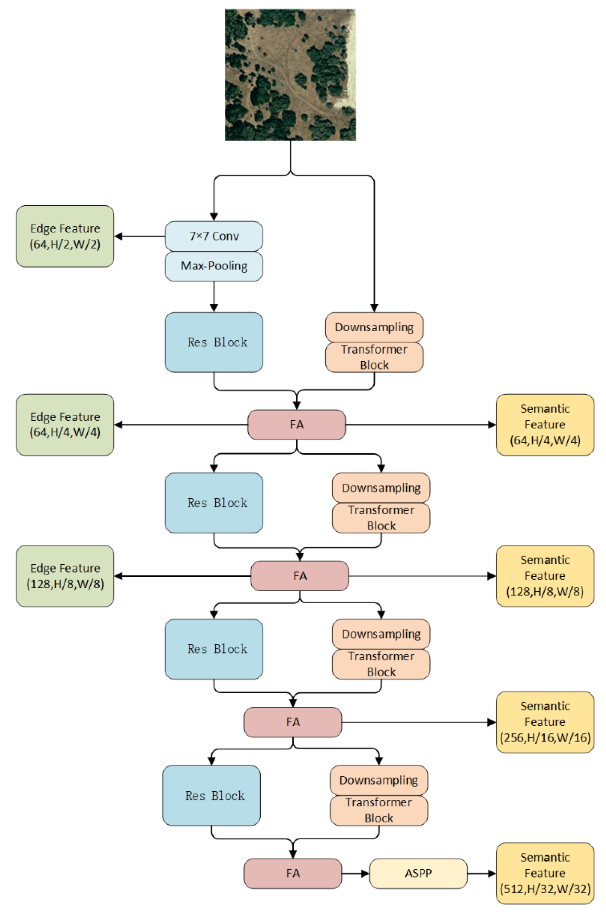
The fusion encoder is shown in Figure 2, which consists of a ResNet encoder [34] and a transformer encoder [30]. The ResNet encoder extracts image features at multiple scales by stacking Residual block, where the n in each downsampling Residual block is 64, 128, 256, or 512, and the number of downsampled Residual block in each layer is 3, 4, 6, and 3. In the first residual block in each residual structure, the stride is taken as 2 to halve the height and width of the feature matrix. The Residual block structure is shown in Figure 3. The convolution branch introduces translation invariance to EGCTNet, and the correlations between local pixels in the image are obtained by sharing the convolution kernel.
The transformer branch encoder consists of four sets of downsampling layers and transformer blocks. The first downsampling layer uses a 3 × 3 Conv2D layer with a kernel size (K) of 7, a stride (S) of 4, and a padding (P) of 3, and the remaining downsampling layers use 3 × 3 Conv2D layers with K = 3, S = 2, and P = 1. The transformer blocks consist of a self-attention module and an MLP layer. Due to the large number of high-resolution image pixels, traditional self-attention modules use a large number of parameters to calculate the image sequence. Sequence reduction [35] can substantially reduce the number of parameters. Sequence reduction can be formulated as follows:
where S represents the original sequence, Reshape represents the shaping operation, R is the reduction rate, H, W, and C are the height, width, and number of channels in the image, respectively, and Linear is the fully connected layer, which reduces the number of channels in S from C · R to C. This process generates a new sequence: .
The generated feature sequence is passed through 2 MLP blocks and a convolutional layer to generate image features that contain global information. The MLP block encodes the feature sequence. In contrast to existing MLP structures, after the first fully connected layer, we convert the sequence to a matrix, perform a convolution, and then convert the matrix back to a sequence. The MLP block is structured as shown in Figure 4.
To combine the image features obtained by the CNN and transformer branches, we use a simple feature aggregator (FA). This feature aggregator is implemented by a 1 × 1 Conv2D layer with K = 1, S = 1, and P = 0, as follows:
where Cat represents the tensor connection, represents the image features obtained by the CNN branch, and represents the image features obtained by the transformer branch.
To enhance multiscale features, we use the atrous spatial pyramid pooling (ASPP) [36] module in the last layer of the encoder. The ASPP module uses Dilated Convolution with different sampling rates, superimposes the different channels using cat, and restores the channels with a 1 × 1 convolution.
2.3. Intermediate Decoder
The intermediate decoder substantially reduces the background noise contained in the features of the ground objects by partially restoring the ground object information. The IMD module is shown in Figure 5. The edge features are obtained from the edge self-attention module, which is introduced in detail in Section 2.5. First, we combine the edge features and mask features and pass the combined features to the deep layer. To aggregate multiscale information when each layer’s edge features are fused with the mask features, we fuse the previous layer’s feature information during each upsampling step. The upsampling operation uses a bilinear interpolation algorithm and skip connections to prevent gradient disappearance. The Edge Embedding Module (EEM) embeds edge information into mask feature matrices of different scales. The EEM outputs the final mask features and passes the mask features to the change decode. The EEM has two main goals.
- (1)
- We downsample the edge features to fit the multiscale fused mask feature structure at each layer; then, we add the features and convolve the output. The details are as follows:where Down is the downsampling operation, is an edge feature, and is a mask feature containing multiscale information.
- (2)
- To prevent gradient disappearance, we retain the direct fusion of the mask and edge features output by the last layer, as follows:where Upsamle is a bilinear interpolation algorithm, is an edge feature, and is a mask feature.
2.4. Change Decoder
The change decoder generates the final change graph, and its structure is shown in Figure 6. The difference module identifies changed features in feature pairs acquired at different scales, and its specific structure is as follows:
where and represent the i-th layer feature maps before and after the change, respectively. Cat is a tensor connection that finds the positional relationship between the features in the feature maps before and after the change at different scales to learn the changed features at different scales. ReLU is the activation function, and BN represents the normalization operation. Considering the offset issues in the image, we did not use the difference between and as the change feature.
Furthermore, to prevent the deep change result from disappearing during gradient descent, the change result of the upper layer is added each time the change feature is calculated. The specific formula is as follows:
where is the variation feature obtained by the deepest EEM in the intermediate decoder, and is the variation feature obtained by the skip-connected EEM in the intermediate decoder.
Next, the variation features obtained by the differential module are uniformly restored to through upsampling. The semantic multiscale feature fusion modules combines 5 groups of changed features, and the fusion process is formulated as follows:
where , , and are the upsampling results of each layer, the upsampling algorithm is bilinear interpolation, Conv2D is a 1 × 1 convolution, and Cat represents the tensor connection.
The fused changed features are upsampled using a transposed convolution to restore the features to their original size and finally passed through a classifier that determines whether each pixel in the matrix has changed.
2.5. Edge Detection Branch
The edge detection branch is used to assist the mask edge of the object in the change detection branch, and its structure is shown in Figure 7. Although the shallow structure contains rich edge information, it also contains complex background noise. Edge self-attention can help shallow features eliminate background noise. Edge self-attention uses deep mask features as a guide to remove noise in shallow features and focus more on ground features. The specific implementation is as follows:
where represents a feature of the ground object mask, represents an edge feature, and Upsample is a bilinear interpolation algorithm that restores the mask feature to the size of the edge feature layer. Sigmoid is the activation function, which is used to obtain the global attention layer containing the ground object mask information. Since the edges are components of the mask features, the dot product between the global attention layer of the feature mask and the edge feature layer can remove background noise in the edge feature layer.
In addition, we take the edge features obtained in the shallowest edge self-attention layer as the edge features in the IMD module. EF is an edge fusion module that fuses the edge features obtained in images at different scales before and after the change. The specific implementation is as follows:
where represents an edge feature in the i-th layer before the change, and represents an edge feature in the i-th layer after the change.
The semantic multiscale feature fusion modules in the edge multiscale feature fusion module and change detection branch have similar structures. We upsample the fused edge features to size and obtain the final edge features by learning the correlations between the edge feature positions at different scales. After the edge feature is restored to size (H, W) through bilinear interpolation, the edge classifier is used to generate the final edge output.
2.6. Loss Function
Our loss function includes the losses of the edge branch and change detection branch and is formulated as follows:
where is the loss that supervises the edge branch, and is the loss that supervises the change detection branch. λ is a regularization parameter that balances the two loss functions. In the experiments performed in this paper, the edge and variation loss weights are balanced when λ = 10.
In the edge task, the edge includes only the outline of a single-pixel object, resulting in a serious imbalance in the numbers of edge and non-edge pixels. Therefore, class-balanced cross-entropy (CBCE) is often used as the loss function in edge tasks and is defined as follows:
where β is the percentage of non-edge pixels in the dataset, which is used to balance the uneven distribution of edge and non-edge pixels in the dataset. is the probability of an edge pixel, and is the probability of a non-edge pixel.
The cross-entropy loss function is commonly used in classification tasks and formulated as follows:
where represents the true value of the i-th pixel, and represents the probability that the predicted value of the i-th pixel is a changed state.
3. Experiments
To verify the effectiveness of EGCTNet, in this section, we explain the datasets, training details, and evaluation indicators used in the experiments, compare existing change detection methods developed in recent years with the proposed network, and analyze the comparison results.
3.1. Datasets and Preprocessing, Implementation Details, Evaluation Metrics, and Comparison Methods
3.1.1. Datasets and Preprocessing
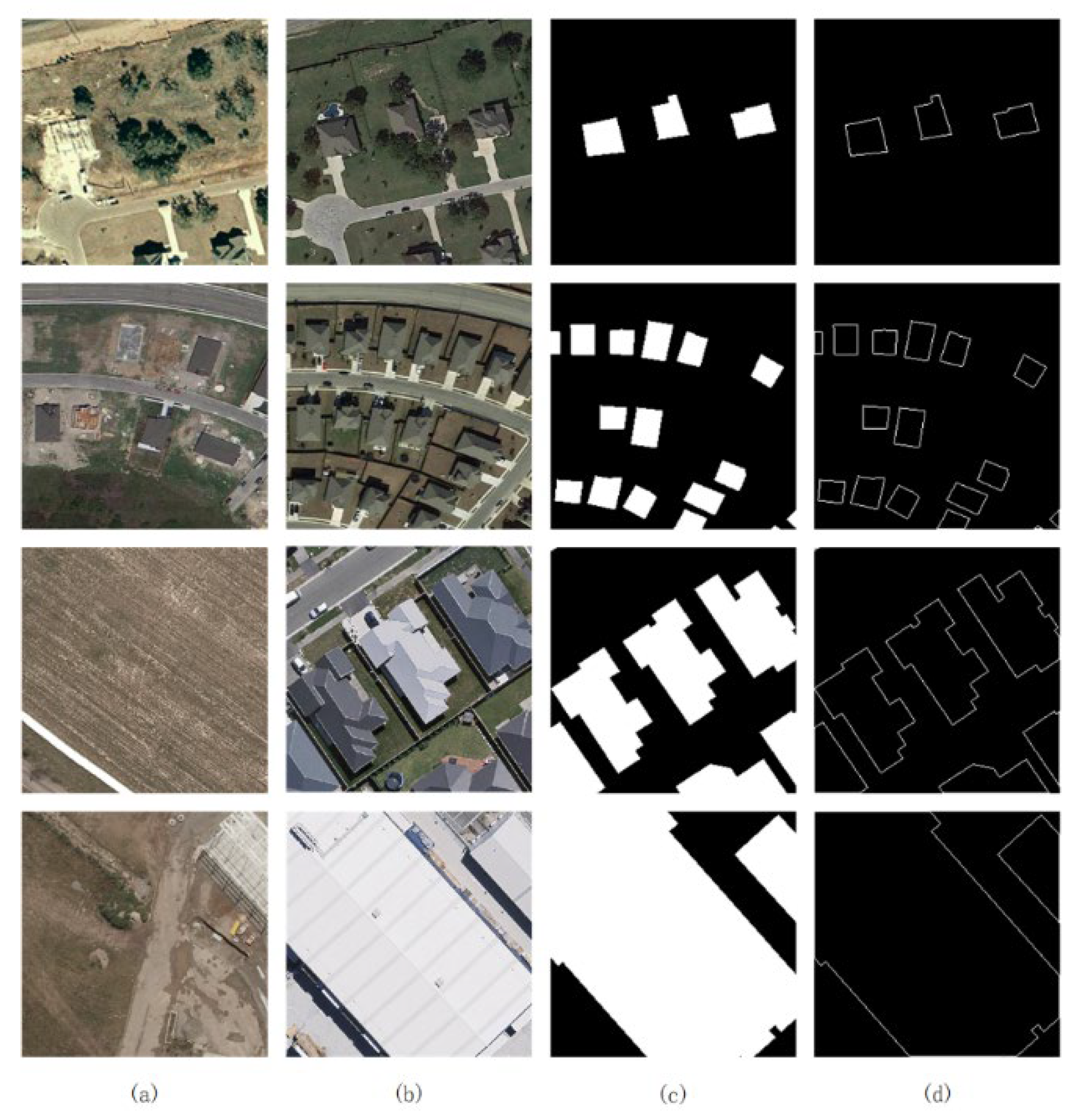
We used two publicly available CD datasets, namely, LEVIR-CD [22] and WHU-CD [37]. Several dataset examples are shown in Figure 8.
LEVIR-CD was acquired by Google Earth between 2002 and 2018, with an image resolution of 0.5 m. This dataset contains 637 pairs of high-resolution remote sensing images of size 1024 × 1024. The LEVIR-CD dataset is used for building change detection, focusing on small and dense buildings with different types of changes.
The authors provided a standard training set, test set, and validation set division for the LEVIR-CD dataset. This experiment follows the original data division and reduces the image size to 256 × 256 according to recent research.
The WHU-CD dataset consists of two sets of aerial data that were acquired in 2012 and 2016, with an image resolution of 0.3 m. This dataset used for building change detection, focusing on large and sparse buildings.
Since the authors did not divide the WHU dataset, we divide the dataset into 7680 nonoverlapping 256 × 256 images and randomly divided the images into training, test, and validation sets at a ratio of 7:2:1.
3.1.2. Implementation Details
We implemented our model in PyTorch and used an NVIDIA RTX 3090 GPU for training. To control for variables, we use the same data augmentation in all methods and use the same hyperparameters as much as possible. During training, we perform data augmentation on the dataset, including random flips, random rescaling (0.8–1.2), random cropping, Gaussian blurs, and random color dithering. The network was randomly initialized at the beginning of training and trained using the AdamW optimizer with beta values of (0.9, 0.999) and a weight decay of 0.01. The learning rate was initially set to 0.0001 and decayed linearly according to the epoch; the batch size was set to 16, and the number of epochs was set to 200.
3.1.3. Evaluation Metrics
In this experiment, we used the F1 and IoU scores of the variation categories as the main quantitative metrics. We also compared the overall accuracy (OA), precision, and recall of the variation categories. These metrics are calculated as follows:
where TP denotes a true positive, TN denotes a true negative, FP denotes a false positive, and FN denotes a false negative.
3.1.4. Comparison Methods
We conduct comparative experiments with several state-of-the-art methods, including 3 methods based on convolutional networks (the fully convolutional Siamese difference method (FC-Siam-Di), fully convolutional Siamese concatenation method (FC-Siam-Conc), and the nest network (NestUnet)), 3 attention-based methods (spatial–temporal attention neural network (STANet), dual-task constrained deep Siamese convolutional network (DTCDSCN), and densely connected Siamese network for change detection (SNUNet)), 1 transformer-based approach (transformer-based Siamese network (ChangeFormer)), and 1 CNN and transformer-based method (bitemporal image transformer (BIT)).
FC-Siam-Di [27]: A change detection method with a CNN structure that encodes multilevel features in bitemporal images and uses feature difference concatenation to obtain change information.
FC-Siam-Conc [27]: A change detection method with a CNN structure that encodes multilevel features in bitemporal images and uses feature fusion concatenation to obtain change information.
NestUnet [38]: A change detection method with a CNN structure that encodes multilevel features in biphasic images and uses feature difference connections to obtain variation information.
STANet [22]: A spatiotemporal attention-based method that calculates the weights of different pixels in space and time to obtain feature information to better distinguish changes.
DTDSCSCN [24]: A channel spatial attention-based approach that uses a dual-attention module (DAM) to improve the model’s ability to discriminate features. We refer to other literature and omit the semantic segmentation decoder to ensure fairness.
SNUNet [39]: A channel attention-based method that applies an ensemble channel attention module (ECAM) to refine the most representative features at different semantic levels for change classification.
ChangeFormer [30]: A transformer-based method that obtains multiscale change information through a transformer encoder and an MLP decoder.
BIT [31]: A method based on convolutions and a transformer that refines convolution features through a transformer decoder and uses feature differences to obtain change information.
3.2. Results on the LEVIR-CD Dataset
On the LEVIR-CD building dataset, we implement all comparison methods except NestUnet using the hyperparameter settings described in the original literature. Since the original author of NestUnet did not conduct experiments on LEVIR-CD, to ensure fairness, the hyperparameter settings of NestUnet are consistent with the hyperparameter settings of our method. The experimental results are shown in Table 1.
Our method achieves the best results on most metrics, with an F1 score of 0.9008 and an IoU score of 0.8295. Our network may benefit from the feature advantages introduced by CNN and transformer fusion coding. Moreover, the addition of the edge detection branch may have improved the IoU score.
As shown in Figure 9, it is worth noting that NestUnet shows excellent performance in the detection of small buildings, which may be because network models with convolutions as their backbone exhibit better local feature extraction. However, the network model with a transformer as its backbone performs better on large building detection. The third set of comparison images in Figure 9 proves our conclusion. EGCTNet combines the advantages of convolutions and transformers. EGCTNet performs well in both small building and large building detection. We use red rectangles to highlight some of the buildings in Figure 9, demonstrating that EGCTNet performs better on the edges of most buildings. However, some buildings are occluded by shadows, which leads to some false detections with EGCTNet.
3.3. Results on the WHU Building Dataset
On the WHU-CD building dataset, to control the hyperparameters, we trained all models except STANet with the same hyperparameters, with a learning rate of 0.0001, a batch size of 16, and 200 epochs. Furthermore, we use AdamW as the optimizer. For STANet, we initially set the batch size to 16; however, the video memory overflowed on our device during training, so we set the batch size of STANet to 4. The final result is shown in the Table 2.
Our method achieves the highest scores on all metrics, with an F1 score of 0.9070 and an IoU score of 0.8298. Since the WHU-CD dataset mainly includes large buildings, these results indicate that our method exhibits better performance than existing methods for change detection of large buildings. Our method also achieves the highest IoU score, showing that our method performs better on building boundaries.
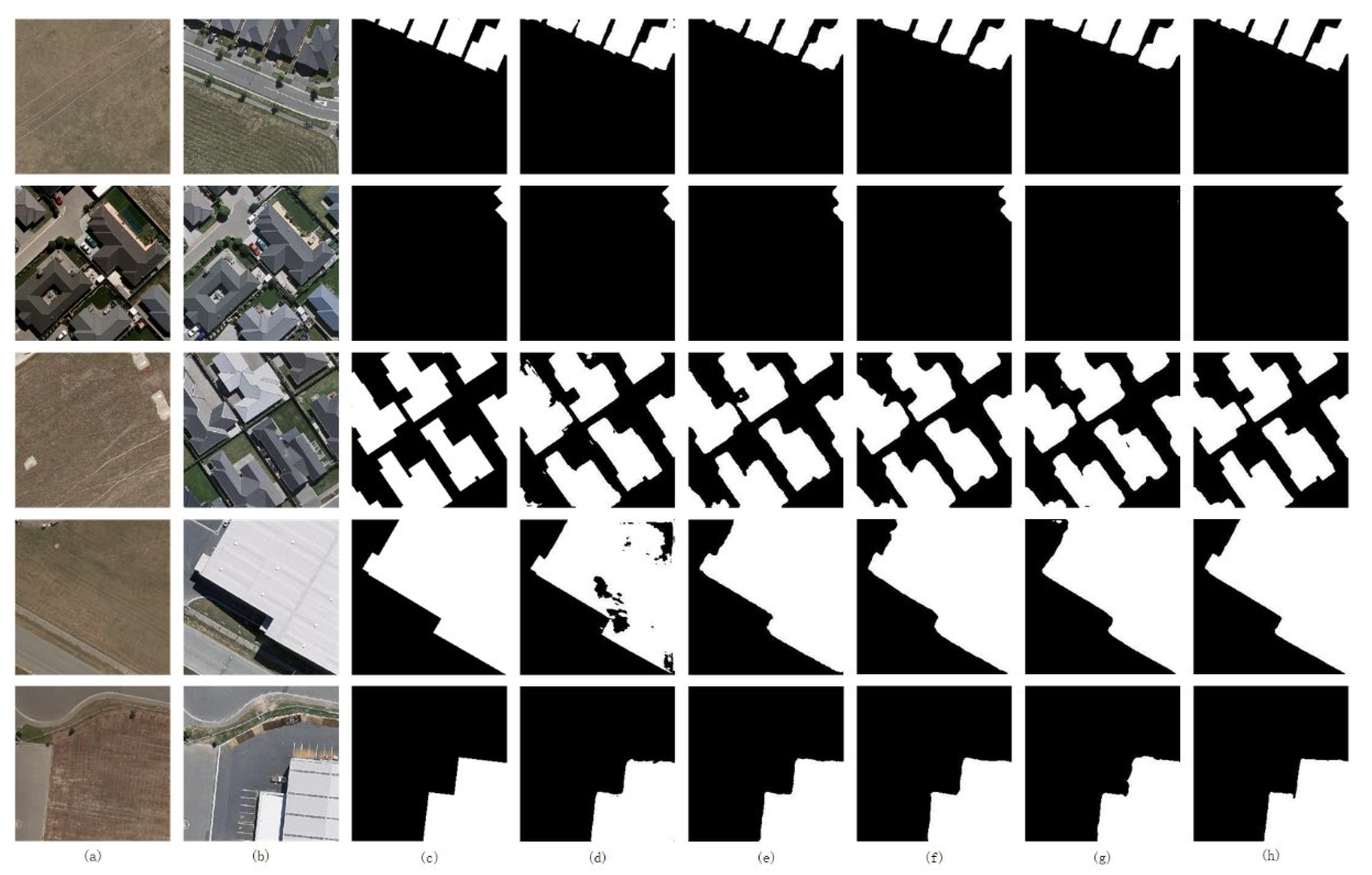
The Figure 10 intuitively shows the performance differences among the different models. NestUnet exhibits good performance in small building change detection, as illustrated by the first and second groups of images in the Figure 10. This result proves that models with CNNs as their backbone network have more significant effects on small buildings due to local correlations in CNNs. However, the fourth set of images shows an issue associated with network models with CNN backbones, which demonstrate poor performance in large building change detection tasks. The performance of BIT, ChangeFormer and EGCTNet in the fourth group of images proves the importance of the global information introduced by the transformer for large building detection. However, using only the transformer as the model backbone results in a loss of features for small buildings, as illustrated by the second set of images. After the edge detection branch is introduced in EGCTNet, the proposed network shows better performance on building boundaries, as illustrated in the Figure 10.
3.4. Ablation Studies
To verify the effectiveness of the fusion encoder, intermediate decoder, and edge detection branch proposed in this paper, we randomly selected 1910 pairs of images in the WHU-CD dataset as the ablation experimental dataset and randomly divided the images in training, test and validation sets. Three sets of comparison networks were designed using a ResNet encoder and change decoder as the basic network structure. The fusion encoder was used in the first group of comparative networks (CTNet), and the second group of comparative networks (CTINet) added an intermediate decoder. In this experiment, we removed edge features with the intermediate decoder. The third group of comparative networks added an edge detection branch, which is the model proposed in this paper. The results are shown in the Table 3.
The second row in the Table 3 shows the result of using the fusion encoder. The F1 score increased from an initial value of 0.8874 to 0.8934, and the IoU score increased from an initial value of 0.7976 to 0.8074. These increases may be because of the global information introduced by the transformer encoder. This global information increases the number of extracted features, improving the overall result. The fusion encoder improves the recall score the most, increasing the recall from 0.8644 to 0.8821, which indicates that more changed pixels are detected in the result. However, the precision is reduced from an initial value of 0.9117 to 0.9050, which may be because the transformer encoder introduces global noise when adding global information, thereby reducing the precision.
The third row in the Table 3 shows the result of adding the intermediate decoder. Compared with the results shown in the second row, all indicators improved. This result proves our argument in Section 2.3. The intermediate decoder considerably reduces the background noise contained in the features of the ground objects by partially restoring the ground object information, thereby improving the detection results.
The fourth row in the Table 3 shows the result of adding the edge branch. Except for the precision, this model achieves the best results in the other indicators, with an IoU of 0.8152 and an F1 score of 0.8982, proving that the edge information introduced by the edge detection branch improves the detection result.
To more intuitively represent the performance difference, we show the results of each comparison network in the Figure 11.
The Figure 11 proves our conclusion. After the transformer coding structure is added to the model, the large building detection performance improves. However, this structure also introduces noise. After the features pass through the intermediate decoder, the excess noise is eliminated. The results of the second and fifth groups in the Figure 11 show this conclusion. Moreover, the method proposed in this paper shows better results at the boundaries than the other methods.
4. Discussion
We provide a completely new approach to change detection. It combines convolution and Transformer for combined encoding, and develops multiple customized modules. Our results are better than some other models (see Figure 9 and Figure 10 and Table 1 and Table 2).
Each module brings different degrees of performance improvement to EGCTNet; but the increase of modules also means the increase of the amount of calculation and parameters. The calculation amount and parameter amount of each module are shown in Table 4.
It can be found that most of the parameters and computations of EGCTNet are due to the use of fused encoders. Compared with the performance improvement brought by the intermediate decoder and edge detection branch, the increased amount of parameters and computation is acceptable. Since the fusion encoder and the encoder in Base only differ in the Transformer structure, the Transformer structure in FE may be the main reason for the increase in the amount of parameters and computation. Although FE brings a larger amount of computation and parameters, the Transformer structure provides a global view for EGCTNet, showing comparatively large advantages in both quantitative and qualitative results (see Figure 11 and Table 3). The fusion encoder combines global features and local features. In the future, we will continue to improve FE, such as using the window idea of the Swim Transformer, to ensure its performance while reducing parameters and computation as much as possible.
5. Conclusions
In this paper, we propose a novel end-to-end change detection network named EGCTNet. After the transformer coding structure is added to the model, EGCTNet shows good performance in detecting large objects. The addition of the intermediate decoder eliminates the global noise introduced by the transformer. The addition of the edge detection branch improves the EGCTNet performance on the edges of objects. The experimental results demonstrate that EGCTNet shows good performance on both small, dense buildings and large, sparse buildings. Thus, our method exhibits good performance for building change detection.
Although the model proposed in this paper achieved good results on multiple datasets, it has some limitations. Since the network introduces both transformer and CNN modules, although we perform sequence reduction on the feature sequence in the transformer module to reduce the computational load, the proposed model still has a larger computational load than existing networks. Multiple custom modules increase the complexity of the model, and at the same time achieve better performance. In future work, we will optimize the calculations in the model to reduce computational costs while ensuring model performance.
Author Contributions
Conceptualization, J.L. and Z.S.; Data curation, J.C., J.Z. and D.Y.; Investigation, J.Z. and D.Y.; Methodology, J.C.; Resources, L.X., J.L. and Z.S.; Supervision, L.X.; Writing—original draft, J.C.; Writing—review & editing, L.X. All authors have read and agreed to the published version of the manuscript.
Funding
This work was supported by the National Key Research and Development Program of China under Grants 2018YFB0505300, the National Science Foundation of China under Grant 41701472, 42071316 and 41971375.
Data Availability Statement
Data associated with this research are available online. The LEVIR-CD dataset is available for download at https://justchenhao.github.io/LEVIR/ (accessed on 23 March 2022). The WHU dataset is available for download at https://study.rsgis.whu.edu.cn/pages/download/building_dataset.html (accessed on 23 March 2022).
Conflicts of Interest
The authors declare no conflict of interest.
References
- Jérôme, T. Change Detection. In Springer Handbook of Geographic Information; Springer: Berlin/Heidelberg, Germany, 2022; pp. 151–159. [Google Scholar]
- Lu, D.; Mausel, P.; Brondizio, E.; Moran, E. Change Detection Techniques. Int. J. Remote Sens. 2004, 25, 2365–2401. [Google Scholar] [CrossRef]
- Hu, J.; Zhang, Y. Seasonal Change of Land-Use/Land-Cover (Lulc) Detection Using Modis Data in Rapid Urbanization Regions: A Case Study of the Pearl River Delta Region (China). IEEE J. Sel. Top. Appl. Earth Obs. Remote Sens. 2013, 6, 1913–1920. [Google Scholar] [CrossRef]
- Jensen, J.R.; Im, J. Remote Sensing Change Detection in Urban Environments. In Geo-Spatial Technologies in Urban Environments; Springer: Berlin/Heidelberg, Germany, 2007; pp. 7–31. [Google Scholar]
- Zhang, J.-F.; Xie, L.-L.; Tao, X.-X. Change Detection of Earthquake-Damaged Buildings on Remote Sensing Image and Its Application in Seismic Disaster Assessment. In Proceedings of the IGARSS 2003. 2003 IEEE International Geoscience and Remote Sensing Symposium. Proceedings (IEEE Cat. No. 03CH37477), Toulouse, France, 21–25 July 2003. [Google Scholar]
- Bitelli, G.; Camassi, R.; Gusella, L.; Mognol, A. Image Change Detection on Urban Area: The Earthquake Case. In Proceedings of the XXth ISPRS Congress, Istanbul, Turkey, 12–23 July 2004. [Google Scholar]
- Dai, X.; Khorram, S. The Effects of Image Misregistration on the Accuracy of Remotely Sensed Change Detection. IEEE Trans. Geosci. Remote Sens. 1998, 36, 1566–1577. [Google Scholar]
- Radke, R.J.; Andra, S.; Al-Kofahi, O.; Roysam, B. Image Change Detection Algorithms: A Systematic Survey. IEEE Trans. Image Process. 2005, 14, 294–307. [Google Scholar] [CrossRef] [PubMed]
- Zhu, J.; Su, Y.; Guo, Q.; Harmon, T. Unsupervised Object-Based Differencing for Land-Cover Change Detection. Photogramm. Eng. Remote Sens. 2017, 83, 225–236. [Google Scholar] [CrossRef]
- Ma, J.; Gong, M.; Zhou, Z. Wavelet Fusion on Ratio Images for Change Detection in Sar Images. IEEE Geosci. Remote Sens. Lett. 2012, 9, 1122–1126. [Google Scholar] [CrossRef]
- Collins, J.B.; Woodcock, C.E. An Assessment of Several Linear Change Detection Techniques for Mapping Forest Mortality Using Multitemporal Landsat Tm Data. Remote Sens. Environ. 1996, 56, 66–77. [Google Scholar] [CrossRef]
- Bovolo, F.; Bruzzone, L. A Theoretical Framework for Unsupervised Change Detection Based on Change Vector Analysis in the Polar Domain. IEEE Trans. Geosci. Remote Sens. 2006, 45, 218–236. [Google Scholar] [CrossRef]
- Chen, Q.; Chen, Y. Multi-Feature Object-Based Change Detection Using Self-Adaptive Weight Change Vector Analysis. Remote Sens. 2016, 8, 549. [Google Scholar] [CrossRef]
- Fung, T.; LeDrew, E. Application of Principal Components Analysis to Change Detection. Photogramm. Eng. Remote Sens. 1987, 53, 1649–1658. [Google Scholar]
- Hussain, M.; Chen, D.; Cheng, A.; Wei, H.; Stanley, D. Change Detection from Remotely Sensed Images: From Pixel-Based to Object-Based Approaches. ISPRS J. Photogramm. Remote Sens. 2013, 80, 91–106. [Google Scholar] [CrossRef]
- Chen, G.; Hay, G.J.; Carvalho, L.M.T.; Wulder, M.A. Object-Based Change Detection. Int. J. Remote Sens. 2012, 33, 4434–4457. [Google Scholar] [CrossRef]
- Lang, S. Object-Based Image Analysis for Remote Sensing Applications: Modeling Reality—Dealing with Complexity. In Object-Based Image Analysis; Springer: Berlin/Heidelberg, Germany, 2008; pp. 3–27. [Google Scholar]
- Chen, G.; Zhao, K.; Powers, R. Assessment of the Image Misregistration Effects on Object-Based Change Detection. ISPRS J. Photogramm. Remote Sens. 2014, 87, 19–27. [Google Scholar] [CrossRef]
- Wan, L.; Xiang, Y.; You, H. A Post-Classification Comparison Method for Sar and Optical Images Change Detection. IEEE Geosci. Remote Sens. Lett. 2019, 16, 1026–1030. [Google Scholar] [CrossRef]
- Ye, S.; Chen, D.; Yu, J. A Targeted Change-Detection Procedure by Combining Change Vector Analysis and Post-Classification Approach. ISPRS J. Photogramm. Remote Sens. 2016, 114, 115–124. [Google Scholar] [CrossRef]
- Zhang, C.; Wei, S.; Ji, S.; Lu, M. Detecting Large-Scale Urban Land Cover Changes from Very High Resolution Remote Sensing Images Using Cnn-Based Classification. ISPRS Int. J. Geo-Inf. 2019, 8, 189. [Google Scholar] [CrossRef]
- Chen, H.; Shi, Z. A Spatial-Temporal Attention-Based Method and a New Dataset for Remote Sensing Image Change Detection. Remote Sens. 2020, 12, 1662. [Google Scholar] [CrossRef]
- Jiang, H.; Hu, X.; Li, K.; Zhang, J.; Gong, J.; Zhang, M. Pga-Siamnet: Pyramid Feature-Based Attention-Guided Siamese Network for Remote Sensing Orthoimagery Building Change Detection. Remote Sens. 2020, 12, 484. [Google Scholar] [CrossRef]
- Liu, Y.; Pang, C.; Zhan, Z.; Zhang, X.; Yang, X. Building Change Detection for Remote Sensing Images Using a Dual-Task Constrained Deep Siamese Convolutional Network Model. IEEE Geosci. Remote Sens. Lett. 2020, 18, 811–815. [Google Scholar] [CrossRef]
- Peng, X.; Zhong, R.; Li, Z.; Li, Q. Optical Remote Sensing Image Change Detection Based on Attention Mechanism and Image Difference. IEEE Trans. Geosci. Remote Sens. 2020, 59, 7296–7307. [Google Scholar] [CrossRef]
- Zheng, Z.; Wan, Y.; Zhang, Y.; Xiang, S.; Peng, D.; Zhang, B. Clnet: Cross-Layer Convolutional Neural Network for Change Detection in Optical Remote Sensing Imagery. ISPRS J. Photogramm. Remote Sens. 2021, 175, 247–267. [Google Scholar] [CrossRef]
- Daudt, R.C.; Saux, B.L.; Boulch, A. Fully Convolutional Siamese Networks for Change Detection. In Proceedings of the 2018 25th IEEE International Conference on Image Processing (ICIP), Athens, Greece, 7–10 October 2018. [Google Scholar]
- Chen, J.; Fan, J.; Zhang, M.; Zhou, Y.; Shen, C. Msf-Net: A Multiscale Supervised Fusion Network for Building Change Detection in High-Resolution Remote Sensing Images. IEEE Access 2022, 10, 30925–30938. [Google Scholar] [CrossRef]
- Bai, B.; Fu, W.; Lu, Y.; Li, S. Edge-Guided Recurrent Convolutional Neural Network for Multitemporal Remote Sensing Image Building Change Detection. IEEE Trans. Geosci. Remote Sens. 2021, 60, 1–13. [Google Scholar] [CrossRef]
- Bandara, W.G.C.; Patel, V.M. A Transformer-Based Siamese Network for Change Detection. arXiv 2022, arXiv:2201.01293. [Google Scholar]
- Chen, H.; Qi, Z.; Shi, Z. Remote Sensing Image Change Detection with Transformers. IEEE Trans. Geosci. Remote Sens. 2021, 60, 1–14. [Google Scholar] [CrossRef]
- Wei, Y.; Zhao, Z.; Song, J. Urban Building Extraction from High-Resolution Satellite Panchromatic Image Using Clustering and Edge Detection. In Proceedings of the IGARSS 2004. 2004 IEEE International Geoscience and Remote Sensing Symposium, Anchorage, AK, USA, 20–24 September 2004. [Google Scholar]
- Jung, H.; Choi, H.-S.; Kang, M. Boundary Enhancement Semantic Segmentation for Building Extraction from Remote Sensed Image. IEEE Trans. Geosci. Remote Sens. 2021, 60, 1–12. [Google Scholar] [CrossRef]
- He, K.; Zhang, X.; Ren, S.; Sun, J. Deep Residual Learning for Image Recognition. In Proceedings of the IEEE Conference on Computer Vision and Pattern Recognition 2016, Las Vegas, NV, USA, 26–30 June 2016. [Google Scholar]
- Sunkara, R.; Luo, T. No More Strided Convolutions or Pooling: A New Cnn Building Block for Low-Resolution Images and Small Objects. arXiv 2022, arXiv:2208.03641. [Google Scholar]
- Chen, L.C.; Papandreou, G.; Kokkinos, I.; Murphy, K.; Yuille, A.L. Deeplab: Semantic Image Segmentation with Deep Convolutional Nets, Atrous Convolution, and Fully Connected Crfs. IEEE Trans. Pattern Anal. Mach. Intell. 2018, 40, 834–848. [Google Scholar] [CrossRef]
- Ji, S.; Wei, S.; Lu, M. Fully Convolutional Networks for Multisource Building Extraction from an Open Aerial and Satellite Imagery Data Set. IEEE Trans. Geosci. Remote Sens. 2018, 57, 574–586. [Google Scholar] [CrossRef]
- Yu, X.; Fan, J.; Chen, J.; Zhang, P.; Zhou, Y.; Han, L. Nestnet: A Multiscale Convolutional Neural Network for Remote Sensing Image Change Detection. Int. J. Remote Sens. 2021, 42, 4898–4921. [Google Scholar] [CrossRef]
- Fang, S.; Li, K.; Shao, J.; Li, Z. Snunet-Cd: A Densely Connected Siamese Network for Change Detection of Vhr Images. IEEE Geosci. Remote Sens. Lett. 2021, 19, 1–5. [Google Scholar] [CrossRef]
Figure 1.
Overall architecture of EGCTNet. The red box is the edge detection branch, FE represents the fusion encoder, ESA represents edge self-attention, IMD represents the intermediate decoder, the blue circle is the edge decoder, EF represents edge fusion, EMFF represents edge multiscale feature fusion, the green circle is the change decoder, DM represents the differential module, and SMFF represents semantic multiscale feature fusion.

Figure 2.
The details of the FE module. Res Block represents the Residual block, FA represents the feature aggregator, and ASPP is an atrous spatial convolution pooling pyramid.
Figure 2.
The details of the FE module. Res Block represents the Residual block, FA represents the feature aggregator, and ASPP is an atrous spatial convolution pooling pyramid.

Figure 3.
The details of Res Block.

Figure 4.
The details of the MLP block.

Figure 5.
The details of the IMD. EEM represents the edge embedding module.

Figure 6.
The details of the change decoder. The red box is the semantic multiscale feature fusion modules.
Figure 6.
The details of the change decoder. The red box is the semantic multiscale feature fusion modules.

Figure 7.
The details of the edge detection branch. The red box is the edge multiscale feature fusion modules.
Figure 7.
The details of the edge detection branch. The red box is the edge multiscale feature fusion modules.

Figure 8.
The first and second rows show cropped examples of the LEVIR-CD dataset, and the third and fourth rows show cropped examples of the WHU dataset. (a) Images before the change. (b) Images after the change. (c) Change label. (d) Change edge label. The images in (d) are generated using the Canny edge detection operator on the images in (c).

Figure 9.
Comparative experimental results on the LEVIR-CD dataset. (a) Pretemporal images. (b) Posttemporal images. (c) Ground truth images. (d) Results of NestUnet. (e) Results of SNUNet. (f) Results of BIT. (g) Results of ChangeFormer. (h) Results of EGCTNet. (Ref boxes highlight areas in the image with significant differences.).

Figure 10.
Comparative experimental results on the WHU-CD dataset. (a) Pretemporal images. (b) Posttemporal images. (c) Ground truth images. (d) Results of NestUnet. (e) Results of DTCDSCN. (f) Results of BIT. (g) Results of ChangeFormer. (h) Results of EGCTNet.
Figure 10.
Comparative experimental results on the WHU-CD dataset. (a) Pretemporal images. (b) Posttemporal images. (c) Ground truth images. (d) Results of NestUnet. (e) Results of DTCDSCN. (f) Results of BIT. (g) Results of ChangeFormer. (h) Results of EGCTNet.

Figure 11.
Results of ablation experiments on the WHU-CD dataset. (a) Pretemporal images. (b) Posttemporal images. (c) Ground truth images. (d) Results of the base model. (e) Results of CTNet. (f) Results of CTINet. (g) Results of EGCTNet. We highlight the differences in the results with red rectangles. (Ref boxes highlight areas in the image with significant differences.).


Table 1.
Quantitative performance comparison on the LEVIR-CD dataset. (The best performance is emphasized in bold.).
Table 1.
Quantitative performance comparison on the LEVIR-CD dataset. (The best performance is emphasized in bold.).
| Method | Precision | Recall | F1 | IoU | OA (%) |
|---|---|---|---|---|---|
| FC-Siam-Di | 0.8953 | 0.8331 | 0.8631 | 0.7592 | 98.67 |
| FC-Siam-Conc | 0.9199 | 0.7677 | 0.8369 | 0.7196 | 98.49 |
| NestUnet | 0.9190 | 0.8806 | 0.8994 | 0.8172 | 98.99 |
| STANet | 0.8381 | 0.9100 | 0.8726 | 0.7740 | 98.66 |
| DTCDSCN | 0.8853 | 0.8683 | 0.8767 | 0.7805 | 98.77 |
| SNUNet | 0.8918 | 0.8717 | 0.8816 | 0.7883 | 98.82 |
| BIT | 0.8924 | 0.8937 | 0.8931 | 0.8068 | 98.92 |
| ChangeFormer | 0.9205 | 0.8880 | 0.9040 | 0.8248 | 99.04 |
| Ours | 0.9220 | 0.8921 | 0.9068 | 0.8295 | 99.06 |
Table 2.
Quantitative performance comparison on the WHU-CD dataset. (The best performance is emphasized in bold.).
Table 2.
Quantitative performance comparison on the WHU-CD dataset. (The best performance is emphasized in bold.).
| Method | Precision | Recall | F1 | IoU | OA (%) |
|---|---|---|---|---|---|
| FC-Siam-Di | 0.8454 | 0.7973 | 0.8206 | 0.6959 | 98.50 |
| FC-Siam-Conc | 0.8596 | 0.7726 | 0.8138 | 0.6860 | 98.48 |
| NestUnet | 0.9285 | 0.8300 | 0.8765 | 0.7801 | 98.99 |
| STANet | 0.8234 | 0.8293 | 0.8263 | 0.7041 | 98.50 |
| DTCDSCN | 0.9315 | 0.8690 | 0.8991 | 0.8168 | 99.16 |
| SNUNet | 0.9143 | 0.8762 | 0.8948 | 0.8097 | 99.11 |
| BIT | 0.9176 | 0.8731 | 0.8948 | 0.8096 | 99.12 |
| ChangeFormer | 0.8841 | 0.8769 | 0.8805 | 0.7865 | 98.98 |
| Ours | 0.9347 | 0.8808 | 0.9070 | 0.8298 | 99.22 |
Table 3.
Accuracy comparison of ablation experiments. (The best performance is emphasized in bold.).
Table 3.
Accuracy comparison of ablation experiments. (The best performance is emphasized in bold.).
| Method | FE | IMD | EDB | WHU-CD (Partial) | ||||
|---|---|---|---|---|---|---|---|---|
| Precision | Recall | F1 | IoU | OA (%) | ||||
| Base | × | × | × | 0.9117 | 0.8644 | 0.8874 | 0.7976 | 96.34 |
| CTNet | ✓ | × | × | 0.9050 | 0.8821 | 0.8934 | 0.8074 | 96.49 |
| CTINet | ✓ | ✓ | × | 0.9068 | 0.8854 | 0.8960 | 0.8116 | 96.57 |
| EGCTNet | ✓ | ✓ | ✓ | 0.9060 | 0.8905 | 0.8982 | 0.8152 | 96.63 |
Table 4.
Params and FLOPs of ablation experiments model.
| Method | FE | IMD | EDB | Params. (M) | FLOPs (G) |
|---|---|---|---|---|---|
| Base | × | × | × | 32.02 | 14.04 |
| CTNet | ✓ | × | × | 57.25 | 21.96 |
| CTINet | ✓ | ✓ | × | 62.80 | 30.02 |
| EGCTNet | ✓ | ✓ | ✓ | 63.26 | 33.52 |
Publisher’s Note: MDPI stays neutral with regard to jurisdictional claims in published maps and institutional affiliations. |
© 2022 by the authors. Licensee MDPI, Basel, Switzerland. This article is an open access article distributed under the terms and conditions of the Creative Commons Attribution (CC BY) license (https://creativecommons.org/licenses/by/4.0/).
Share and Cite
MDPI and ACS Style
Xia, L.; Chen, J.; Luo, J.; Zhang, J.; Yang, D.; Shen, Z. Building Change Detection Based on an Edge-Guided Convolutional Neural Network Combined with a Transformer. Remote Sens. 2022, 14, 4524. https://doi.org/10.3390/rs14184524
AMA Style
Xia L, Chen J, Luo J, Zhang J, Yang D, Shen Z. Building Change Detection Based on an Edge-Guided Convolutional Neural Network Combined with a Transformer. Remote Sensing. 2022; 14(18):4524. https://doi.org/10.3390/rs14184524
Chicago/Turabian StyleXia, Liegang, Jun Chen, Jiancheng Luo, Junxia Zhang, Dezhi Yang, and Zhanfeng Shen. 2022. "Building Change Detection Based on an Edge-Guided Convolutional Neural Network Combined with a Transformer" Remote Sensing 14, no. 18: 4524. https://doi.org/10.3390/rs14184524
Note that from the first issue of 2016, this journal uses article numbers instead of page numbers. See further details here.