
Marine Oil Spill Detection with X-Band Shipborne Radar Using GLCM, SVM and FCM
by
 , ,
, ,
Bo Li
1, 
Jin Xu
1,*,
Xinxiang Pan
1,
Long Ma
1,
Zhiqiang Zhao
1,
Rong Chen
1,
Qiao Liu
1 and
Haixia Wang
2 1
Maritime College, Guangdong Ocean University, Zhanjiang 524088, China
2
Navigation College, Dalian Maritime University, Dalian 116026, China
*
Author to whom correspondence should be addressed.
Remote Sens. 2022, 14(15), 3715; https://doi.org/10.3390/rs14153715
Submission received: 27 June 2022
/
Revised: 22 July 2022
/
Accepted: 1 August 2022
/
Published: 3 August 2022
(This article belongs to the Special Issue Remote Sensing of Interaction between Human and Natural Ecosystem)
Abstract
:Marine oil spills have a significant adverse impact on the economy, ecology, and human health. Rapid and effective oil spill monitoring action is extraordinarily important for controlling marine pollution. A marine oil spill detection scheme based on X-band shipborne radar image with machine learning is proposed here. First, the original shipborne radar image collected on Dalian 7.16 oil spill accident was transformed into a Cartesian coordinate system and noise suppressed. Then, texture features and SVM were used to indicate the effective monitoring location of ocean waves. Third, FCM was applied to classify the oil films and ocean waves. Finally, the oil spill detection result was transformed back to a polar coordinate system. Compared with an improved active contour model and another oil spill detection method with SVM, our method performed more intelligently. It can provide data support for marine oil spill emergency response.

1. Introduction
Oil spill accidents have become more frequent with the rapid development of coastal port cities [1]. An oil spill has a great adverse impact on the environment, ecology, economy, and human health [2,3]. On 27 April 2021, for example, the general cargo ship Sea justice of Panama collided with the anchored oil tanker Symphony of Libya off the coast of Qingdao Port, China, causing a major oil spill accident in the Yellow Sea [4]. Marine oil spill pollution spreads speedily and widely [5,6]. Rapid and effective oil spill monitoring and early warning are of great significance for the prevention and control of marine disasters [7,8].
At present, remote sensing sensors used in the field of oil spill monitoring can be installed on satellites, aircraft, and ships. Spaceborne remote sensing sensors can detect large-scale marine oil films. This deployment scheme can be conducive to large-scale oil spill monitoring. Chen et al. [9] established an oil spill segmentation framework by using the synchronization of SAR images. By re-studying the SAR imaging mechanism, they obtained the image probability distribution representation for oil spill segmentation. Rousso et al. [10] suggested an oil spill detection method based on image filtering technique and convolutional neural network (CNN), which proved accurate in satellite SAR images. Wang et al. [11] used ResNet-18 as the backbone of DeepLabv3+ encoder to improve a Deep Learning model of oil leak detection in the RADARSAT-2 SAR image, which showed fine performance. Almulihi et al. [12] proposed a novel online nonparametric Bayesian analysis method for SAR image oil spill detection based on the infinite Gamma mixture model. The determination of cluster number is bypassed via an infinite number of mixed components. Rajendran et al. [13] used Sentinel-1 and Sentinel-2 data obtained before, during, and after the accident to assess the Wakashio oil spill accident impact in the Indian Ocean near Mauritius on 6 August 2020, to understand the spread of the oil spill on the coastal environment. Rao et al. [14] used the Sentinel-1 SAR imagery to track and delineate the oil spills and the affected coastal areas of Mauritius.
Airborne sensor oil spill monitoring technology is developing rapidly because of its convenient application. Liu et al. [15] used spectral indices-based band selection (SIS) and convolutional neural networks to auto-classify oil films in airborne visible infrared imaging spectrometer (AVIRIS) high spectral remote sensing images. Chen and Lu [16] combined subcategory perceptual feature selection and SVM classifier to recognize oil films in remote sensing images of optical cameras on unmanned aerial vehicles or aircraft.
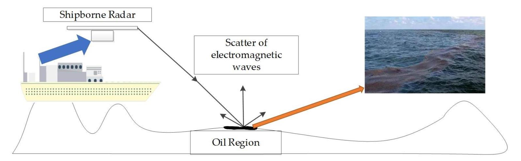
The rapid development of spaceborne and airborne oil spill monitoring technology provides valuable experience for the promotion of shipborne oil spill monitoring technology. The highlight target detection range of shipborne radar can reach 24 nautical miles. The oil spill shows relatively dark characteristics in the wave echo area. When the effective ocean wave echo image of the sea surface is fine, the oil spill detection distance can reach more than 1 nautical mile. The shipborne radar has an important application prospect in oil spill detection, because of its convenience and low cost. However, due to less research, this technology is still in the early stage [17]. Based on shipborne radar images collected from Dalian 7.16 oil spill accident, scholars from Dalian Maritime University have continuously published oil spill detection technology research since 2015 [18,19,20,21,22,23,24,25,26,27]. Zhu et al. [18] put forward a manual marine oil spill extraction method with a shipborne image gray correction technique. Liu et al. [19] applied an iterative adaptive threshold method to determine oil spill targets in the shipborne radar image. Xu et al. [20] proposed the dual-threshold method to survey the oil spill information in the shipborne radar image after screening the effective ocean wave monitoring regions. Xu et al. [28] improved an active contour model (ACM) to detect oil film targets from shipborne radar images after gray correction.
In this paper, an offshore oil film detection method is proposed with Gray-Level Co-occurrence Matrix (GLCM), Support Vector Machine (SVM), and Fuzzy C-Means (FCM). After data preprocessing, GLCM and SVM are used to select the effective regions of wave monitoring. FCM is used to classify marine oil films. The organization of this paper is composed as follows: The experimental shipborne radar image and related theoretical methods are given in Section 2. Section 3 presents the experimental results. Section 4 shows the analysis, discussion, and comparisons. Finally, the conclusions are summarized in Section 5.
2. Materials and Methods
2.1. Dataset
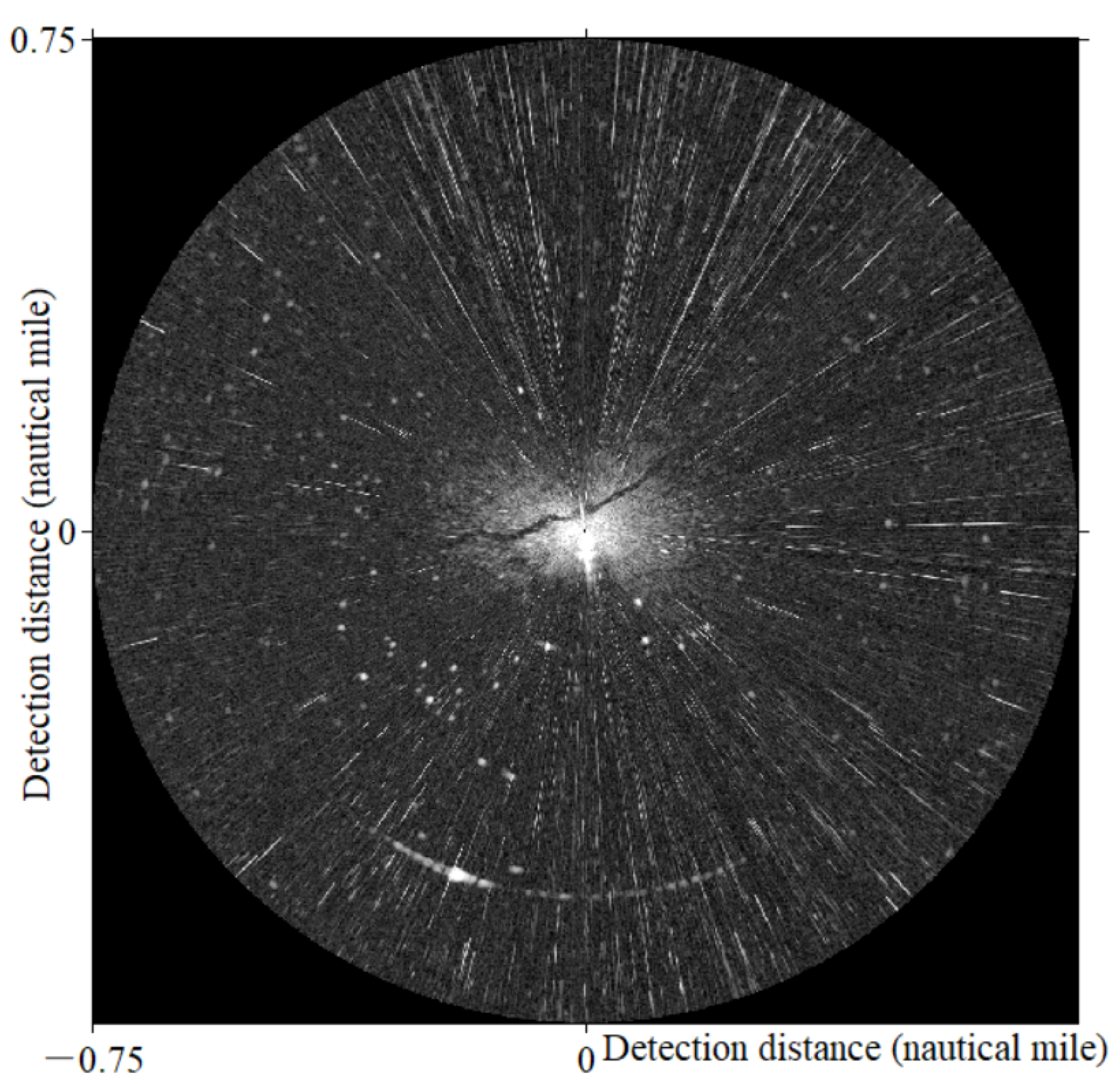
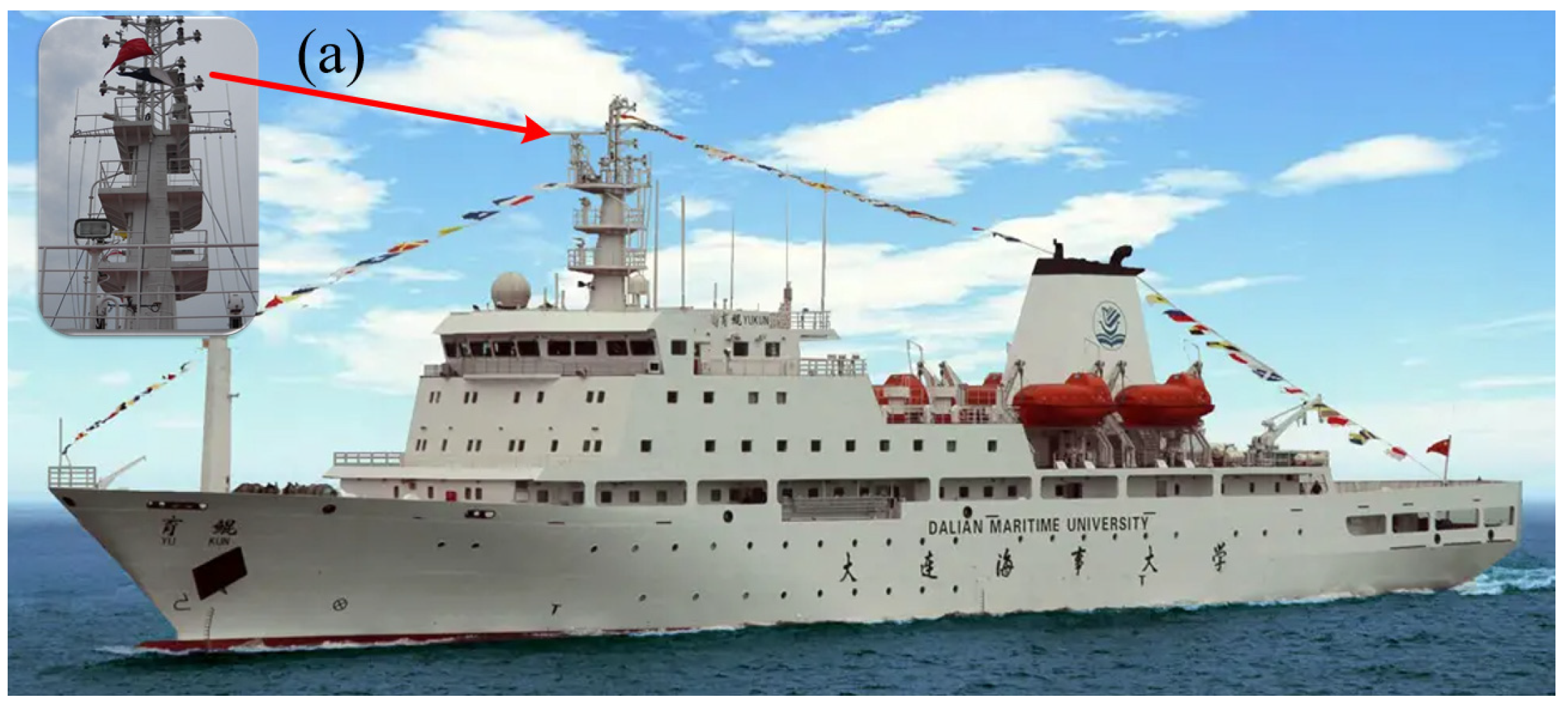
The experimental data (Figure 1) used here was acquired from the teaching-practice ship Yukun (Figure 2) of Dalian Maritime University in the Dalian 7.16 oil spill accident on 21 July 2010. The 7.16 accident caused a large amount of crude oil pollution near the sea. The radar image size was 1024 × 1024 pixels. The actual image detection range was 0.75 nautical miles. The shipborne radar-specific parameters are shown in Table 1.
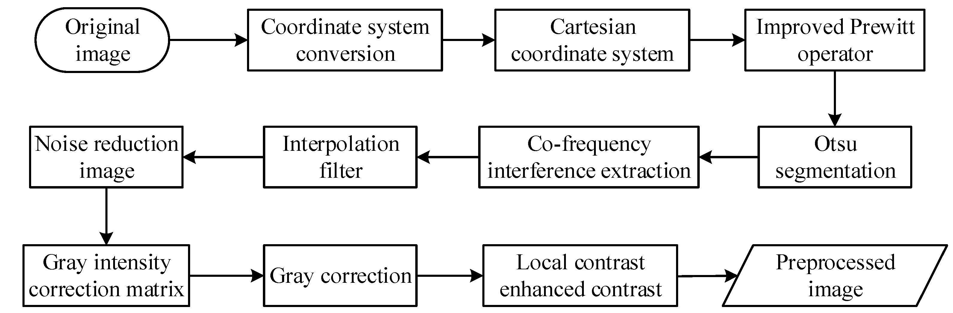
2.2. Data Preprocessing
2.3. Methods
2.3.1. GLCM
GLCM is a second-order statistical method used to calculate the frequency of pixel pairs with the same gray scales and study spatial correlation characteristics for image texture [29]. It expresses the comprehensive information in sub-image, direction, and gradient. It is also defined as a two-dimensional matrix of joint probabilities between pairs of pixels, separated by a given distance d in a preset direction θ [30,31,32].
Haralick defined 14 statistical features from the GLCM for texture classification. The feature “Contrast” was selected here for our research. Contrast measures the intensity linking contrast between a pixel and its neighbor. It is defined as:
where N = 256 denotes the number of gray levels for 8-bit image, while (i, j) indicates cell location of the GLCM, and p(i, j) is the cell value at (i, j). In our study, the textural features were generated from 64 × 64 sub-images.
2.3.2. SVM
SVM [33] is a generalized linear classifier for binary classification by supervised learning. The decision boundary is the maximum-margin hyperplane for learning samples, as shown in Figure 5. In the shipborne radar image, the effective wave echo pixels are distributed around the hull. As the detection distance increases, the effective pixels of the wave echo gradually decrease due to the distance attenuation or scattering characteristics. SVM is used here to classify effective ocean wave monitoring regions and background.
2.3.3. FCM
FCM is a classical unsupervised fuzzy clustering algorithm [34,35], which divides the data into c number categories according to the membership degrees of the clustered data for solving optimization problems. Given a dataset X = {x1, x2, …, xn} with the c number of different clusters, FCM has the following objective function:
where 1 ≤ k ≤ n and 1 ≤ i ≤ c. m denotes a fuzzy degree with m > 1. uik represents a membership degree of xk generated from the ith cluster. dik is the distance between xk and vi as:
The alternating iterative method and the Lagrangian multiplier are employed to solve the constrained optimization problem. Then, uik and vi can be given as:
When the iteration process converges by computing uik and vi, the optimal solution of Jm can be obtained. FCM was used here to segment rough results of oil films.
2.3.4. ACM
Chan and Vese [36] proposed an active contour for image segmentation. A gray image I(x): Ω→R is divided into the target Rin and background Rout, starting with a preset contour C with the energy:
where Cin and Cout are gray intensity constants of Rin and Rout, respectively.
Li et al. [37] proposed an improved region-based ACM with the energy as:
where λ1 and λ2 are as previously defined. f1(x) and f2(x) are spatially varying fitting functions. Furthermore, K is a kernel function with the localization property of K(u) decreases and approaches zero as |u| increases. A Gaussian kernel was chosen as K(x) with a standard deviation of σ into the ACM:
Xu et al. [28] proposed an area threshold parameter D(x) to improve LBF model:
where A is the area of continuous pixels, Tin and Tout are the area thresholds of Rin and Rout, respectively.
3. Results
3.1. Local Window Feature Extraction
The preprocessed image was cut with 64 × 64 pixels local window size. Each local window was assigned the feature value according to the Contrast of GLCM, as shown in Figure 6.
3.2. Effective Sea Wave Monitoring Regions Extraction
3.3. Oil films Identificaiton
FCM was used to divide Figure 8 into 3 classes after 15 iterations as Figure 9a. The class with the lowest value was multiplied by Figure 7 as the rough oil films segmentation, as shown in Figure 9b. After that, the speckles and false positive targets caused by the ship’s wake were deleted to obtain the oil film identification result as Figure 10. This process takes 26.71 s on average. Finally, the identification result is transformed into the polar coordinate system as Figure 11.
4. Discussion
4.1. Selection of Local Window Size
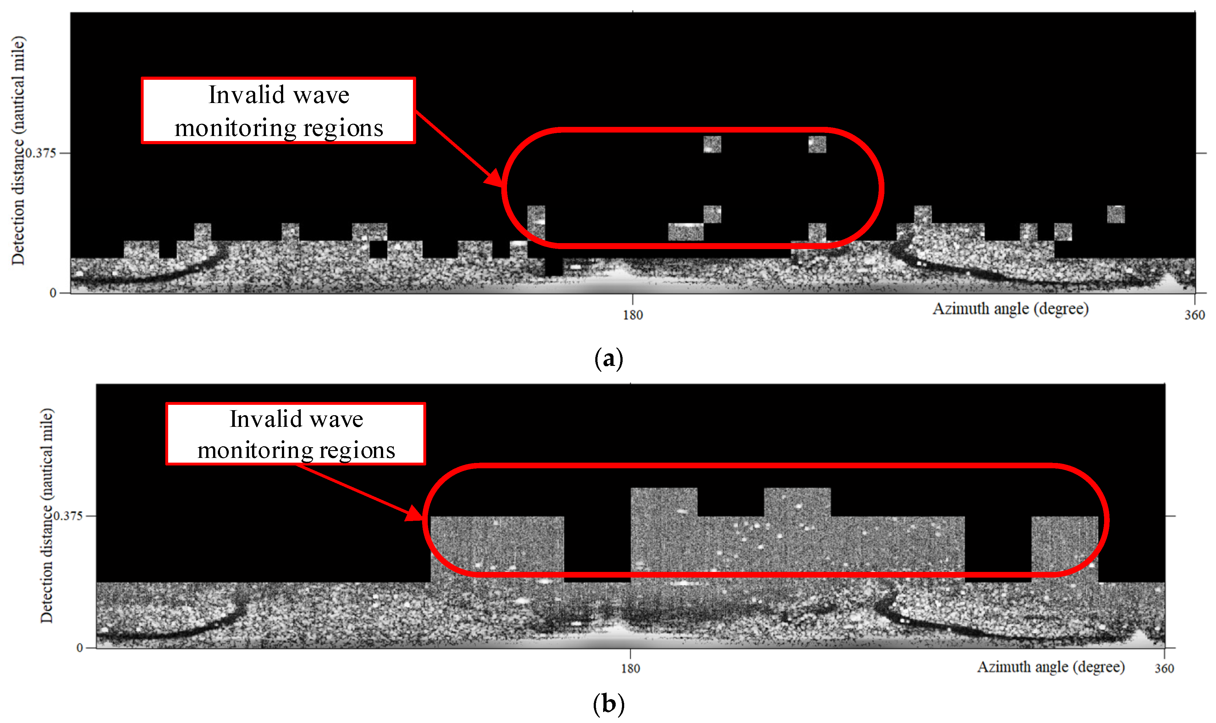
Effective ocean wave monitoring regions calculated by different local window sizes of 32 × 32 pixels and 128 × 128 pixels were shown in Figure 12. Different time consumption was shown in Table 2. The small local window size mode consumes more calculation time. The computational efficiency improved as the local window size increased. So, a larger local window size should be recommended first for the application of emergency treatment sites. However, our method with the local window sizes of 32 × 32 pixels and 128 × 128 pixels contained invalid wave monitoring regions, which may lead to detecting false oil spill targets as in Figure 12a,b. Compared with these two local window sizes, it was suggested that the combined application of 64 × 64 pixels local window size, GLCM, and SVM was more suitable for extracting the effective areas of ocean wave monitoring.
4.2. Selection of GLCM Features
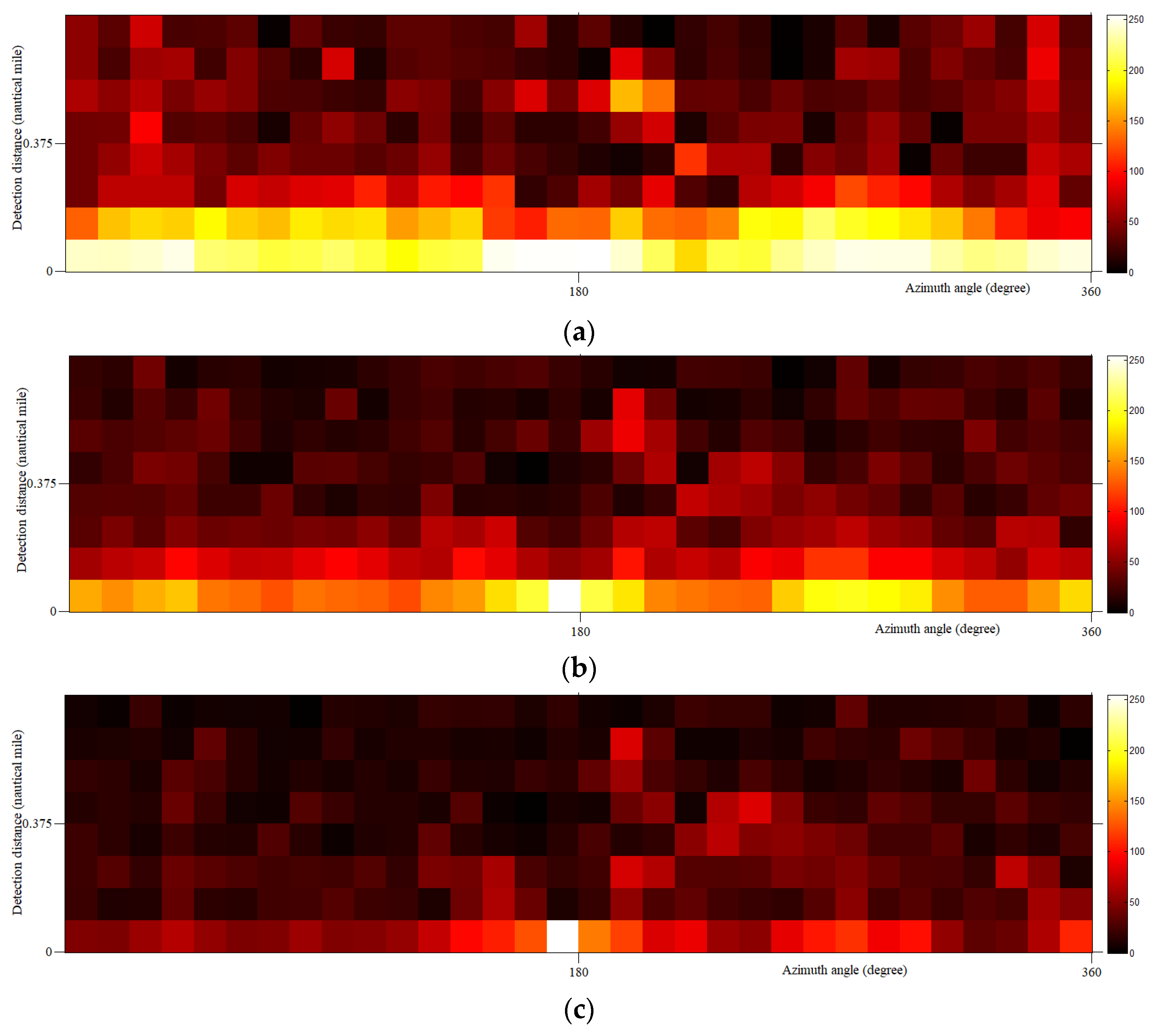
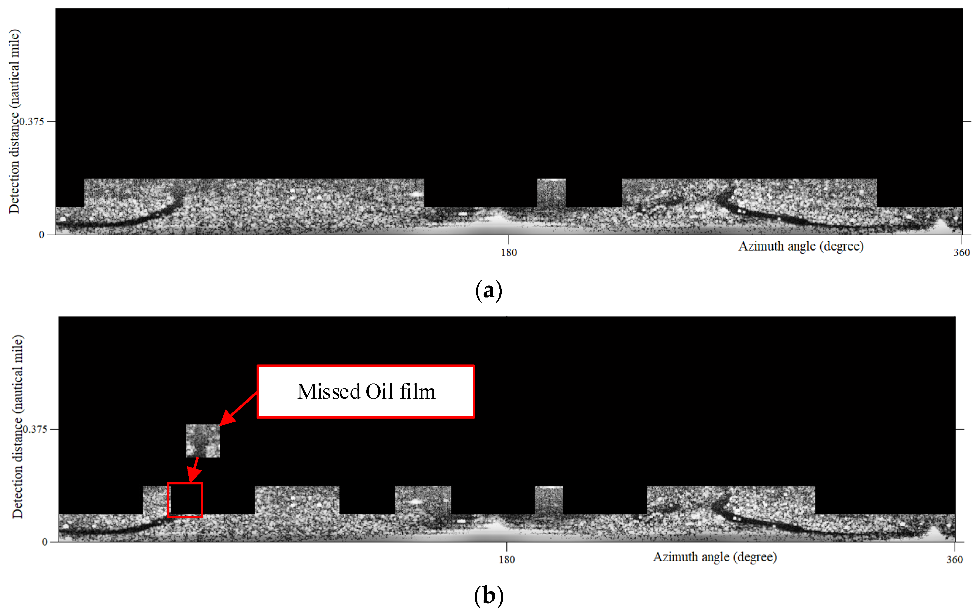
The applicability of wave area screening was compared by using the Correlation, Energy, Homogeneity and Contrast of GLCM features, as shown in Figure 13. The off-set distance d was set to 1 pixel, the direction θ was set to horizontal. In order to improve the computational efficiency, the gray level of the shipborne radar image is compressed to a smaller range without affecting the texture features. So, the number of gray levels was set to eight. As the gray level changes from 256 to 8, the image appears dim. However, it has little effect on texture features information extraction. Local windows containing ocean waves show a low Contrast value in Figure 6, a high Correlation value in Figure 13a, and a high Homogeneity value in Figure 13b. By using features of Correlation and Homogeneity, similar results were obtained with the Contrast feature, as shown in Figure 14. However, a small oil film region was missed in Figure 14b. So, the Homogeneity feature had some defects for wave area screening. Because of the uneven distribution of feature values in Figure 13c, the Energy feature is not suitable for oil film extraction of our preprocessed image. Therefore, Contrast and Correlation features were suggested here for screening effective ocean wave regions.
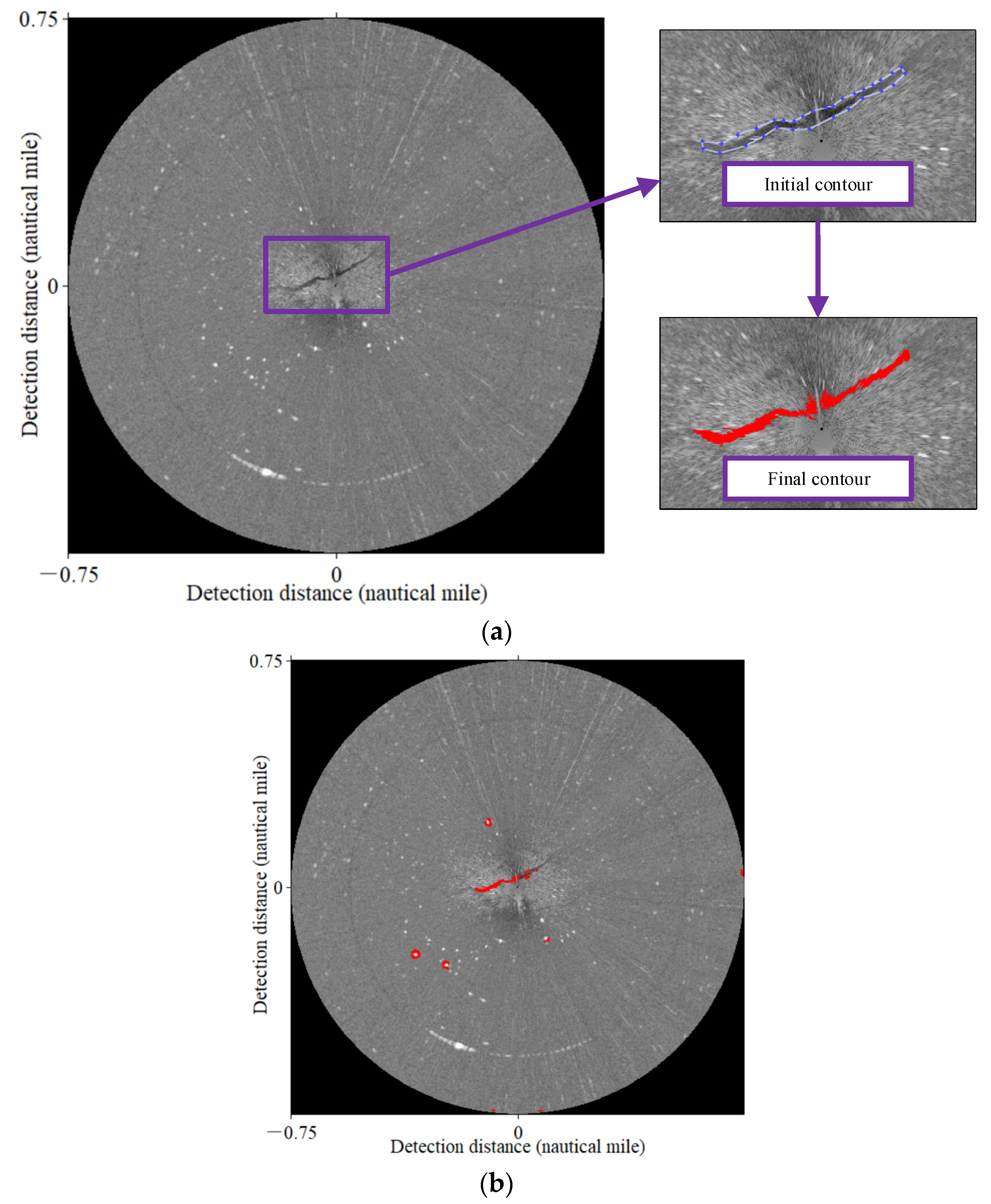
4.3. Comparation with An Improved ACM
Xu et al. [28] proposed an improved ACM (Method 2) to identify oil film targets in shipborne radar images after gray correction. ACM method needs to preset an initial contour to achieve the purpose of target segmentation. Their shipborne radar image data preprocessing included noise reduction and gray adjustment. So, in order to compare with Method 2 in the same image, Figure 4f was transformed here into a polar coordinate system as Figure 15. Through their experimental comparison of Method 2, the oil film extraction effect was better when λ1 = 1, λ2 = 2, σ = 3. The above parameter values of Method 2 were used for experiments. When the number of iterations exceeded 10, the results tended to be stable. Therefore, we set i (iteration) = 20. As the image was sampled locally, Method 2 can obtain similar results as our method (Figure 15a). It showed high efficiency for iterating 20 times only in 1.49 s. However, the result was not ideal when extracting oil films from the whole image, as shown in Figure 15b. Moreover, with the calculation of the whole image, it took 7.78 s to iterate 20 times. Due to the iterative computation of the FCM classification process, our method took 32.89 s. Compared with our method, Method 2 showed higher efficiency, especially in local windows. However, our method can be applied to the whole graph without manual operation.
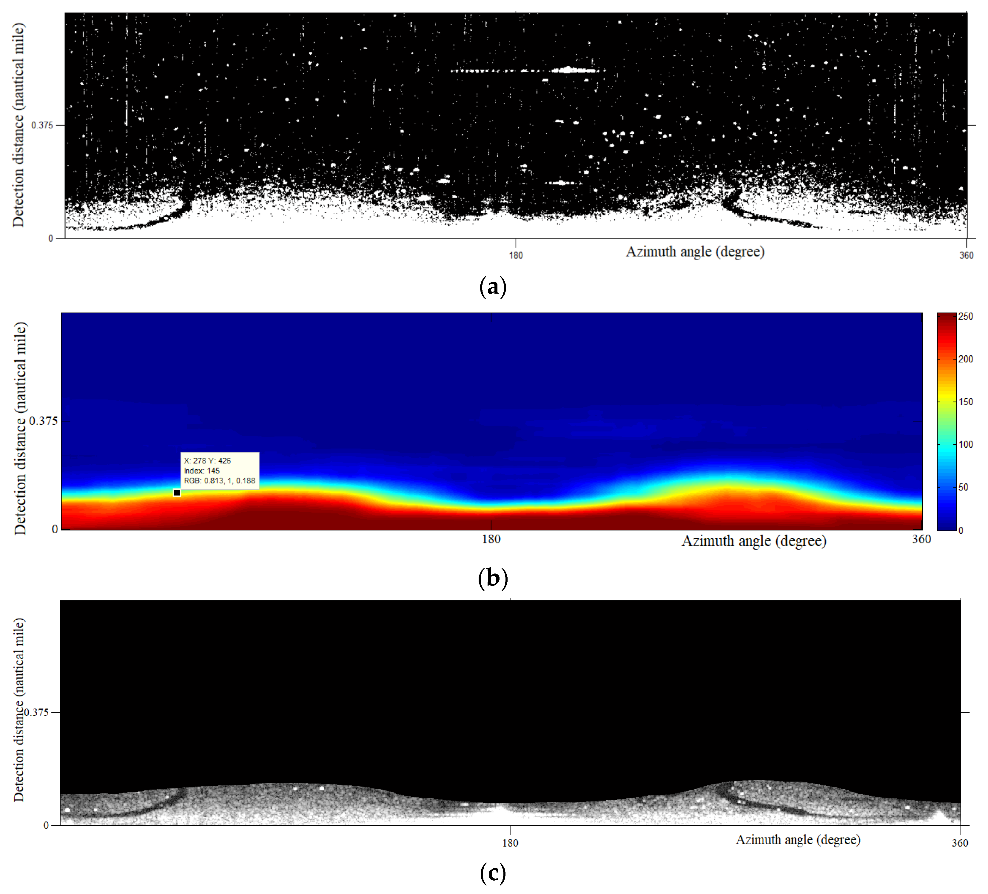
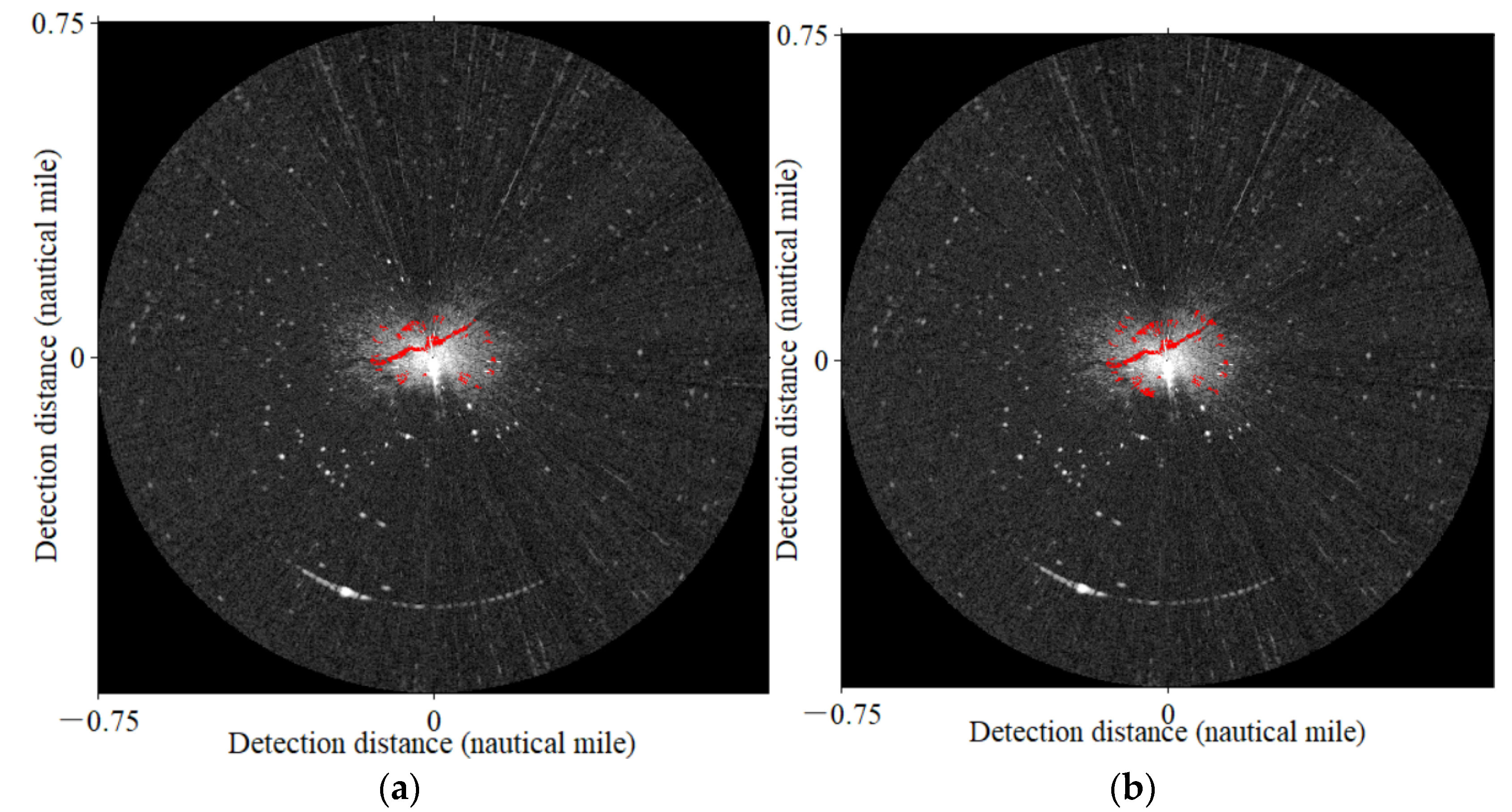
4.4. Comparation with Another Oil Film Detection Method with SVM and Adaptive Threshold
Xu et al. [23] put forward an oil film detection scheme (Method 3) in shipborne radar images using SVM and an improved adaptive threshold. Method 3 is first to screen out the effective monitoring areas containing wave pixels around the hull by using SVM and gray distribution matrix and then accurately extract the offshore oil films combined with the local adaptive threshold. Method 3 was used to compare our method with the same noise reduction image (Figure 4d). At the beginning, the SVM of Method 3 was used to classify the ocean wave pixels and background of the preprocessed image as Figure 16a. Then, the gray distribution matrix (Figure 16b) of Method 3 and a manual threshold were applied to divide effective ocean wave monitoring regions as in Figure 16c. At last, an improved adaptive threshold method of Method 3 was used to detect oil spills as in Figure 17. The threshold in Figure 16b needed to be manually selected in the gray distribution matrix through expert experience for wave effective regions screening. Different thresholds may result in distinct oil film detection results. If the threshold was manually selected as 145 in the experiment (Figure 16b), the result of Method 3 was shown in Figure 17a. If the threshold was manually selected as 100, the result was shown in Figure 17b. This process of manually selecting thresholds of Method 3 in Figure 16b leads to unstable detection results. Nevertheless, our method used texture features and SVM to determine the effective monitoring of ocean wave range without manual intervention, which performed more intelligently. Moreover, the oil spill classification result was more stable.
5. Conclusions
A marine oil spill detection method was proposed in this paper. After data preprocessing, GLCM and SVM were used to screen the effective ocean sea monitoring regions. Then, FCM was applied to classify the oil films. In the process of oil spill extraction and result generation, our method adopts twice image coordinate system transformations. The detection of oil spills on the sea surface by shipborne radar depends on the effect of oil film restraining wave pixels (relatively dark image feature) and striped morphology. So, intelligent screening of effective ocean wave monitoring regions plays an important role in our method. False positive detection of oil film targets will be caused by the incorrect division of effective ocean wave monitoring regions.
At present, our method is suitable for detecting thick and non-volatile oil films. In future work, we will carry out classification experiments for different kinds of oil films with different thicknesses. This automatic segmentation method can be performed onboard a response ship operationally to provide effective data support for offshore oil spill emergency disposal.
Author Contributions
Conceptualization, B.L. and J.X.; methodology, X.P. and Z.Z.; software, L.M. and R.C.; validation, Q.L. and Z.Z., H.W. and J.X.; formal analysis, B.L.; investigation, L.M.; resources, J.X.; data curation, L.M.; writing—original draft preparation, B.L. All authors have read and agreed to the published version of the manuscript.
Funding
This research was funded by the National Natural Science Foundation of China, grant number 52071090; the Natural Science Foundation of Guangdong Province, grant number 2022A1515011603; the Special projects in key fields (Artificial Intelligence) of Universities in Guangdong Province, grant number 2019KZDZX1035; the Research start-up funding project of Guangdong Ocean University, grant number 060302132009.
Data Availability Statement
The experimental shipborne radar image was collected by scholars of Dalian Maritime University. The participants did not agree to share their data publicly.
Conflicts of Interest
The authors declare no conflict of interest.
References
- Kieu, H.T.; Law, A.W.K. Remote sensing of coastal hydro-environment with portable unmanned aerial vehicles (pUAVs) a state-of-the-art review. J. Hydro-Environ. Res. 2021, 37, 32–45. [Google Scholar] [CrossRef]
- Yang, Y.Q.; Li, Y.; Li, J.; Liu, J.G.; Gao, Z.Y.; Guo, K.X.; Yu, H. The influence of Stokes drift on oil spills: Sanchi oil spill case. Acta Oceanol. Sin. 2021, 40, 30–37. [Google Scholar] [CrossRef]
- Oliveira, L.G.; Araujo, K.C.; Barreto, M.C.; Bastos, M.E.P.A.; Lemos, S.G.; Fragoso, W.D. Applications of chemometrics in oil spill studies. Microchem. J. 2021, 166, 106216. [Google Scholar] [CrossRef]
- Kim, T.; Shin, H.K.; Jang, S.Y.; Ryu, J.M.; Kim, P.; Yang, C.S. Calculation Method of Oil Slick Area on Sea Surface Using High-resolution Satellite Imagery: M/V Symphony Oil Spill Accident. Korean J. Remote Sens. 2021, 37, 1773–1784. [Google Scholar]
- Dearden, C.; Culmer, T.; Brooke, R. Performance measures for validation of oil spill dispersion models based on satellite and coastal data. IEEE J. Ocean. Eng. 2022, 44, 126–140. [Google Scholar] [CrossRef]
- Dasari, K.; Anjaneyulu, L.; Nadimikeri, J. Application of C-band sentinel-1A SAR data as proxies for detecting oil spills of Chennai, East Coast of India. Mar. Pollut. Bull. 2022, 174, 113182. [Google Scholar] [CrossRef]
- Mohammadiun, S.; Hu, G.J.; Gharahbagh, A.A.; Li, J.B.; Hewage, K.; Sadiq, R. Intelligent computational techniques in marine oil spill management: A critical review. J. Hazard. Mater. 2021, 419, 126425. [Google Scholar] [CrossRef]
- Jafarzadeh, H.; Mahdianpari, M.; Homayouni, S.; Mohammadimanesh, F.; Dabboor, M. Oil spill detection from Synthetic Aperture Radar Earth observations: A meta-analysis and comprehensive review. GIScience Remote Sens. 2021, 58, 1022–1051. [Google Scholar] [CrossRef]
- Chen, F.; Zhang, A.H.; Balzter, H.; Ren, P.; Zhou, H.Y. Oil spill SAR image segmentation via probability distribution modeling. IEEE J. Sel. Top. Appl. Earth Obs. Remote Sens. 2022, 15, 533–554. [Google Scholar] [CrossRef]
- Rousso, R.; Katz, N.; Sharon, G.; Glizerin, Y.; Kosman, E.; Shuster, A. Automatic recognition of oil spills using neural networks and classic image processing. Water 2022, 14, 1127. [Google Scholar] [CrossRef]
- Wang, D.; Wan, J.; Liu, S.; Chen, Y.; Yasir, M.; Xu, M.; Ren, P. BO-DRNet: An improved deep learning model for oil spill detection by polarimetric features from SAR images. Remote Sens. 2022, 14, 264. [Google Scholar] [CrossRef]
- Almulihi, A.; Alharithi, F.; Bourouis, S.; Alroobaea, R.; Pawar, Y.; Bouguila, N. Oil spill detection in SAR images using online extended variational learning of Dirichlet Process Mixtures of Gamma Distributions. Remote Sens. 2021, 13, 2991. [Google Scholar] [CrossRef]
- Rajendran, S.; Vethamony, P.; Sadooni, F.N.; Al-Kuwari, H.A.; Al-Khayat, J.A.; Seegobin, V.O.; Govil, H.; Nasir, S. Detection of Wakashio oil spill off Mauritius using Sentinel-1 and 2 data: Capability of sensors, image transformation methods and mapping. Environ. Pollut. 2021, 274, 116618. [Google Scholar] [CrossRef]
- Rao, V.T.; Suneel, V.; Alex, M.J.; Gurumoorthi, K.; Thomas, A.P. Assessment of MV Wakashio oil spill off Mauritius, Indian Ocean through satellite imagery: A case study. J. Earth Syst. Sci. 2022, 131, 21. [Google Scholar] [CrossRef]
- Liu, B.; Li, Y.; Li, G.; Liu, A. A Spectral Feature based Convolutional Neural Network for classification of sea surface oil spill. ISPRS Int. J. Geo-Inf. 2019, 8, 160. [Google Scholar] [CrossRef] [Green Version]
- Chen, T.; Lu, S.J. Subcategory-Aware Feature Selection and SVM optimization for automatic aerial image-based oil spill inspection. IEEE Trans. Geosci. Remote Sens. 2017, 55, 5264–5273. [Google Scholar] [CrossRef]
- Chen, P.; Zhou, H.; Li, Y.; Liu, B.; Liu, P. Oil spill identification in radar images using a soft attention segmentation model. Remote Sens. 2022, 14, 2180. [Google Scholar] [CrossRef]
- Zhu, X.Y.; Li, Y.; Feng, H.; Liu, B.X.; Xu, J. Oil spill detection method using X-band marine radar imagery. J. Appl. Remote Sens. 2015, 9, 095985. [Google Scholar] [CrossRef]
- Liu, P.; Li, Y.; Xu, J.; Zhu, X.Y. Adaptive enhancement of X-band marine radar imagery to detect oil spill segments. Sensors 2017, 17, 2349. [Google Scholar] [CrossRef] [Green Version]
- Xu, J.; Liu, P.; Wang, H.; Lian, J.J.; Li, B. Marine radar oil spill monitoring technology based on dual-threshold and C-V level set methods. J. Indian Soc. Remote Sens. 2018, 46, 1949–1961. [Google Scholar] [CrossRef]
- Xu, J.; Cui, C.; Feng, H.Y.; You, D.M.; Wang, H.X.; Li, B. Marine radar oil spill monitoring through local adaptive thresholding. Environ. Forensics 2019, 20, 196–209. [Google Scholar] [CrossRef]
- Liu, P.; Li, Y.; Liu, B.; Chen, P.; Xu, J. Semi-Automatic oil spill detection on X-band marine radar images using texture analysis, machine learning, and adaptive thresholding. Remote Sens. 2019, 11, 756. [Google Scholar] [CrossRef] [Green Version]
- Xu, J.; Wang, H.; Cui, C.; Zhao, B.G.; Li, B. Oil spill monitoring of shipborne radar image features using SVM and Local Adaptive Threshold. Algorithms 2020, 13, 69. [Google Scholar] [CrossRef] [Green Version]
- Liu, P.; Li, Y.; Xu, J.; Wang, T. Oil spill extraction by X-band marine radar using texture analysis and adaptive thresholding. Remote Sens. Lett. 2019, 1, 583–589. [Google Scholar] [CrossRef]
- Xu, J.; Pan, X.X.; Jia, B.B.; Wu, X.X.; Liu, P.; Li, B. Oil spill detection using LBP feature and K-Means clustering in shipborne radar image. J. Mar. Sci. Eng. 2021, 9, 65. [Google Scholar] [CrossRef]
- Xu, J.; Jia, B.Z.; Pan, X.X.; Li, R.H.; Cao, L.; Cui, C.; Wang, H.H.; Li, B. Hydrographic data inspection and disaster monitoring using shipborne radar small range images with electronic navigation chart. PeerJ Comput. Sci. 2020, 6, e290. [Google Scholar] [CrossRef] [PubMed]
- Xu, J.; Pan, X.X.; Wu, X.R.; Jia, B.Z.; Fei, J.; Wang, H.X.; Li, B.; Cui, C. Oil spill discrimination of multi-time-domain shipborne radar images using active contour model. Geosci. Lett. 2021, 8, 7. [Google Scholar] [CrossRef]
- Xu, J.; Wang, H.; Cui, C.; Liu, P.; Zhao, Y.; Li, B. Oil spill segmentation in shipborne radar images with an improved active contour model. Remote Sens. 2019, 11, 1698. [Google Scholar] [CrossRef] [Green Version]
- Haralick, R.M.; Shanmugam, K.; Dinstein, I. Textural features for image classification. IEEE Trans. Syst. Man Cybern. 1973, SMC-3, 610–621. [Google Scholar] [CrossRef] [Green Version]
- Benco, M.; Hudec, R.; Kamencay, P.; Zachariasova, M.; Matuska, S. An advanced approach to extraction of colour texture features based on GLCM. Int. J. Adv. Robot. Syst. 2014, 11, 104. [Google Scholar] [CrossRef]
- Iqbal, N.; Mumtaz, R.; Shafi, U.; Zaidi, S.M.H. Gray level co-occurrence matrix (GLCM) texture based crop classification using low altitude remote sensing platforms. PeerJ Comput. Sci. 2021, 7, e536. [Google Scholar] [CrossRef] [PubMed]
- Tamal, M. A Phantom Study to Investigate Robustness and Reproducibility of Grey Level Co-Occurrence Matrix (GLCM)-Based Radiomics Features for PET. Appl. Sci. 2021, 11, 535. [Google Scholar] [CrossRef]
- Cortes, C.; Vapnik, V. Support-vector networks. Mach. Learn 1995, 20, 273–297. [Google Scholar] [CrossRef]
- Bezdek, J.C. Pattern Recognition with Fuzzy Objective Function Algorithms; Plenum: New York, NY, USA, 1981. [Google Scholar]
- Gan, H. Safe Semi-Supervised Fuzzy C-Means Clustering. IEEE Access 2019, 7, 95659–95664. [Google Scholar] [CrossRef]
- Chan, T.F.; Vese, L.A. Active contours without edges. IEEE Trans. Image Process. 2001, 10, 266–277. [Google Scholar] [CrossRef] [PubMed] [Green Version]
- Li, C.M.; Kao, C.Y.; Gore, J.C.; Ding, Z. Minimization of regionscalable fitting energy for image segmentation. IEEE Trans. Image Process. 2008, 17, 1940–1949. [Google Scholar] [CrossRef] [Green Version]
Figure 1.
Experimental image.

Figure 2.
The experimental data acquisition platform. (a) The shipborne radar installation position.
Figure 2.
The experimental data acquisition platform. (a) The shipborne radar installation position.

Figure 3.
The data preprocessing scheme.

Figure 4.
The preprocessed image. (a) Original image in Cartesian coordinate system; (b) Improved Prewitt operator convolution; (c) Otsu segmentation; (d) Interpolation filter noise reduction; (e) Gray intensity correction matrix; (f) Image grayscale adjustment; (g) Local contrast-enhanced contrast.


Figure 5.
Optimal hyperplane for binary classification. The yellow line in the middle is the classification hyperplane. The points on the two black dotted lines are the points closest to the hyperplane, and these points are support vectors.
Figure 5.
Optimal hyperplane for binary classification. The yellow line in the middle is the classification hyperplane. The points on the two black dotted lines are the points closest to the hyperplane, and these points are support vectors.

Figure 6.
Contrast characteristic value of local window.

Figure 7.
SVM Classification result of effective ocean wave monitoring regions. Some remote misclassification regions had been deleted.
Figure 7.
SVM Classification result of effective ocean wave monitoring regions. Some remote misclassification regions had been deleted.

Figure 8.
Result of effective ocean wave monitoring regions.

Figure 9.
Rough oil films segmentation result. (a) FCM classification; (b) Rough segmentation result.
Figure 9.
Rough oil films segmentation result. (a) FCM classification; (b) Rough segmentation result.

Figure 10.
Fine oil films segmentation result.

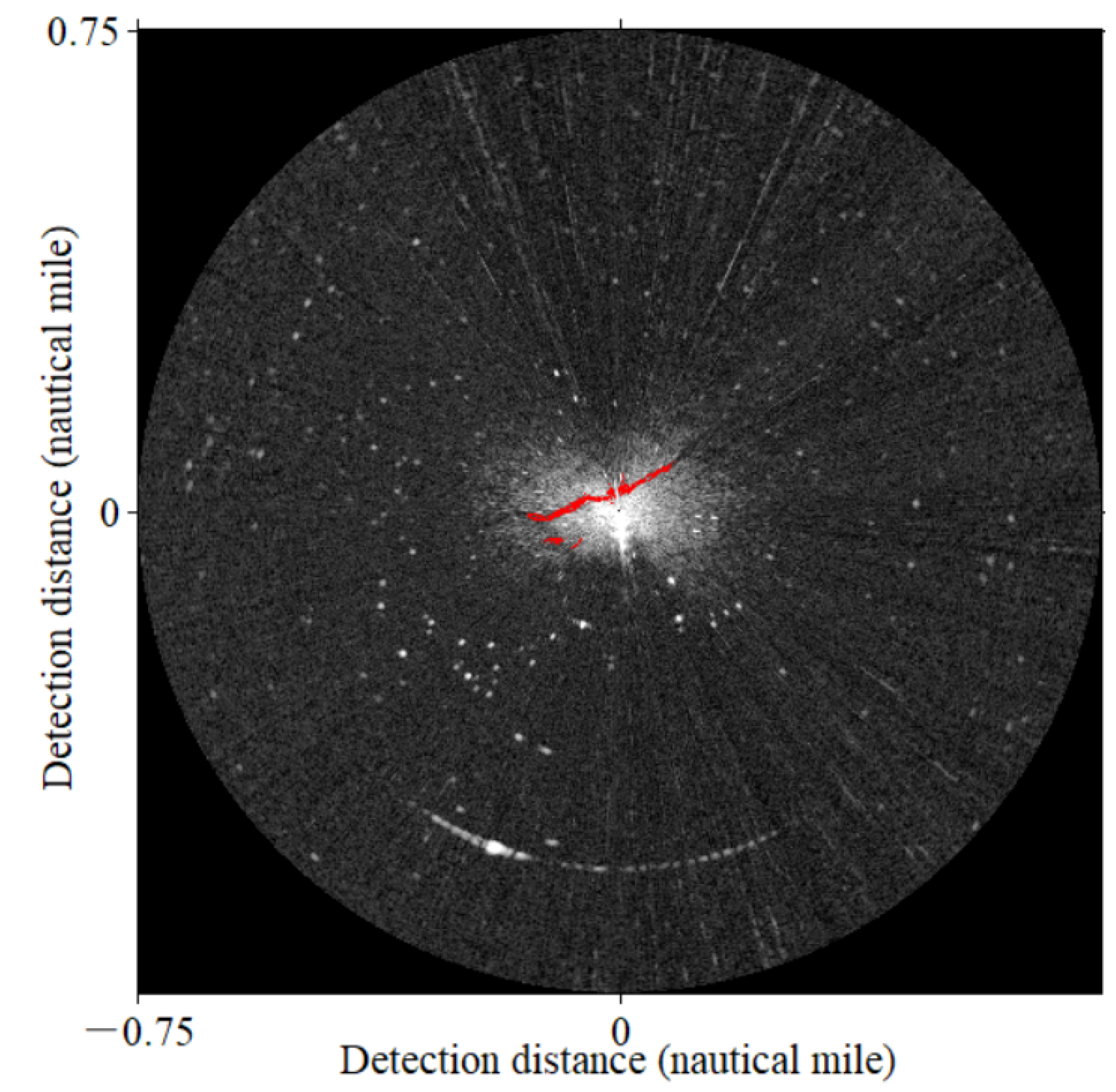
Figure 11.
Oil films segmentation results in the polar coordinate system. The oil films were marked in red.
Figure 11.
Oil films segmentation results in the polar coordinate system. The oil films were marked in red.

Figure 12.
Effective ocean wave monitoring regions calculated by different local window sizes. (a) 32 × 32 pixels; (b) 128 × 128 pixels.
Figure 12.
Effective ocean wave monitoring regions calculated by different local window sizes. (a) 32 × 32 pixels; (b) 128 × 128 pixels.

Figure 13.
Different GLCM feature maps of preprocessed image. (a) Correlation; (b) Homogeneity; (c) Energy.
Figure 13.
Different GLCM feature maps of preprocessed image. (a) Correlation; (b) Homogeneity; (c) Energy.

Figure 14.
Effective area screening for ocean wave monitoring by using Correlation and Homogeneity of GLCM features. (a) Correlation; (b) Homogeneity. Red square with oil film had been removed in Homogeneity feature classification.
Figure 14.
Effective area screening for ocean wave monitoring by using Correlation and Homogeneity of GLCM features. (a) Correlation; (b) Homogeneity. Red square with oil film had been removed in Homogeneity feature classification.

Figure 15.
Results of Method 2. (a) Contour extraction after image sampling; (b) Contour extraction in the whole image. The segmentation results were marked in red.
Figure 15.
Results of Method 2. (a) Contour extraction after image sampling; (b) Contour extraction in the whole image. The segmentation results were marked in red.

Figure 16.
The threshold in the gray distribution matrix was manually selected to determine the effective monitoring range of ocean wave. (a) SVM classification results of ocean wave; (b) Segmentation threshold was manually selected; (c) The ocean wave monitoring range was divided according to the threshold ‘145’.

Figure 17.
Results of Method 3. (a) The selected threshold in the gray distribution matrix was ‘145’; (b) The selected threshold in the gray distribution matrix was ‘100’. The segmentation results were marked in red.
Figure 17.
Results of Method 3. (a) The selected threshold in the gray distribution matrix was ‘145’; (b) The selected threshold in the gray distribution matrix was ‘100’. The segmentation results were marked in red.


Table 1.
The shipborne radar-specific parameters.
| Parameter Name | Parameter Value |
|---|---|
| Product manufacturer and model | Sperry Marine B.V. |
| Electromagnetic spectrum | X-band |
| Pulse repetition frequency | 3000 Hz/1800 Hz/785 Hz |
| Pulse width | 50 ns/250 ns/750 ns |
| Video image range | 0.5/0.75/1.5/3/6/12 NM |
| Antenna type | Waveguide split antenna |
| Antenna length | 8 ft |
| Polarization mode | Horizontal |
| Horizontal detection angle | 360° |
| Rotation speed | 28–45 revolutions/min |
Table 2.
Time consumed for extracting effective monitoring regions of ocean waves with different local window sizes.
Table 2.
Time consumed for extracting effective monitoring regions of ocean waves with different local window sizes.
| Local Window Size | Tiles Generation (s) | Feature Map Generation (s) | SVM Classification (s) | Summary (s) |
|---|---|---|---|---|
| 32 × 32 | 2.08 | 19.62 | 1.11 | 22.81 |
| 64 × 64 | 0.53 | 4.75 | 0.98 | 6.26 |
| 128 × 128 | 0.20 | 1.53 | 0.96 | 2.69 |
Publisher’s Note: MDPI stays neutral with regard to jurisdictional claims in published maps and institutional affiliations. |
© 2022 by the authors. Licensee MDPI, Basel, Switzerland. This article is an open access article distributed under the terms and conditions of the Creative Commons Attribution (CC BY) license (https://creativecommons.org/licenses/by/4.0/).
Share and Cite
MDPI and ACS Style
Li, B.; Xu, J.; Pan, X.; Ma, L.; Zhao, Z.; Chen, R.; Liu, Q.; Wang, H. Marine Oil Spill Detection with X-Band Shipborne Radar Using GLCM, SVM and FCM. Remote Sens. 2022, 14, 3715. https://doi.org/10.3390/rs14153715
AMA Style
Li B, Xu J, Pan X, Ma L, Zhao Z, Chen R, Liu Q, Wang H. Marine Oil Spill Detection with X-Band Shipborne Radar Using GLCM, SVM and FCM. Remote Sensing. 2022; 14(15):3715. https://doi.org/10.3390/rs14153715
Chicago/Turabian StyleLi, Bo, Jin Xu, Xinxiang Pan, Long Ma, Zhiqiang Zhao, Rong Chen, Qiao Liu, and Haixia Wang. 2022. "Marine Oil Spill Detection with X-Band Shipborne Radar Using GLCM, SVM and FCM" Remote Sensing 14, no. 15: 3715. https://doi.org/10.3390/rs14153715
Note that from the first issue of 2016, this journal uses article numbers instead of page numbers. See further details here.