
A Spatial–Spectral Joint Attention Network for Change Detection in Multispectral Imagery


1
School of Computer Science and Technology, Xi’an University of Posts and Telecommunications, Xi’an 710121, China
2
Shaanxi Key Laboratory of Network Data Analysis and Intelligent Processing, Xi’an 710121, China
3
Xi’an Key Laboratory of Big Data and Intelligent Computing, Xi’an 710121, China
4
The Department of Electronic Engineering, Chengdu University of Information Technology, Chengdu 610103, China
5
The Key Laboratory of Spectral Imaging Technology CAS, Xi’an Institute of Optics and Precision Mechanics, Chinese Academy of Sciences, Xi’an 710119, China
*
Author to whom correspondence should be addressed.
Remote Sens. 2022, 14(14), 3394; https://doi.org/10.3390/rs14143394
Submission received: 26 May 2022
/
Revised: 30 June 2022
/
Accepted: 12 July 2022
/
Published: 14 July 2022
(This article belongs to the Section Remote Sensing Image Processing)
Abstract
:Change detection determines and evaluates changes by comparing bi-temporal images, which is a challenging task in the remote-sensing field. To better exploit the high-level features, deep-learning-based change-detection methods have attracted researchers’ attention. Most deep-learning-based methods only explore the spatial–spectral features simultaneously. However, we assume the key spatial-change areas should be more important, and attention should be paid to the specific bands which can best reflect the changes. To achieve this goal, we propose the spatial–spectral joint attention network (SJAN). Compared with traditional methods, SJAN introduces the spatial–spectral attention mechanism to better explore the key changed areas and the key separable bands. To be more specific, a novel spatial-attention module is designed to extract the spatially key regions first. Secondly, the spectral-attention module is developed to adaptively focus on the separable bands of land-cover materials. Finally, a novel objective function is proposed to help the model to measure the similarity of learned spatial–spectral features from both spectrum amplitude and angle perspectives. The proposed SJAN is validated on three benchmark datasets. Comprehensive experiments have been conducted to demonstrate the effectiveness of the proposed SJAN.
1. Introduction
Different images of the same location acquired at two or more different times are referred to as multi-temporal images. The variations between multi-temporal remote-sensing images can be identified by change detection. Change-detection method determines if each pixel in a scene has changed by extracting changed areas from multi-temporal images. Multispectral images have numerous bands, ranging from visible to infrared light, and their extensive spectral information allows for reliable object identification. As a result, multispectral change detection has found widespread application in the fields of environmental monitoring [1,2,3,4], resource inquiry [5,6,7], urban planning [8,9,10], and natural catastrophe assessment [11,12,13].
The two primary categories of change-detection methods are traditional and deep-learning-based methods. For low-resolution images, the earliest change-detection methods mostly used pixels as the monitoring unit and carried out pixel-by-pixel difference analysis. With the development of machine-learning algorithms and the increase in spectral resolution, the unit of change detection shifted from pixels to objects. Prior to 2010, the majority of these technologies were traditional change-detection methods, which consist of algebra-based, image-transform-based, classification-based methods, and so on [14]. Change detection based on algebraic and image transforms detects changes in images by applying transformations and operations to image pixels. While the post-classification method classifies two temporal-phase remote-sensing images that have been aligned separately in advance, and then compares the classification results to obtain change-detectionmaps.
Although the above traditional methods have made important contributions to the development of multispectral change detection, most of them still use manual features and rely on professional visual observers for manual discrimination. Deep learning can automatically extract abstract features and obtain spatial–spectral feature representation, which can effectively improve the accuracy of change-detection tasks. Therefore, deep-learning-based change-detection methods have become a popular research direction. With the continuous improvement of satellite-remote-sensing image resolution, the change-detection methods based on deep learning have also made a qualitative leap in the extraction of multispectral image features. There are various network structures that have been applied in the field of change detection, such as deep-belief networks (DBN) [15], stacked auto-encoders (SAE) [16], convolutional auto-encoders (CAE) [17], PCANet [18].
Some methods aim at extracting spatial–spectral features to obtain a better performance concerning the change detection. Zhan et al. [19] proposed a three-way spectral–spatial convolutional neural network (TDSSC), which used convolution to extract spectral features from the spectral direction and spectral–spatial features from the spatial direction to fully extract HSI discriminative features, improving the accuracy of change detection. Zhang et al. [20] proposed a novel unsupervised change-detection method based on spectral transformation and joint spectral–spatial feature learning (STCD). It overcame the challenge of the same object image with different spectra in multiple spatial–temporal periods and improved the robustness of the change-detection method. Liu et al. [21] introduced a dual-attention module (DAM) to exploit the interdependencies between channels and spatial positions. The method could obtain more discriminative features and the authors conducted experiments on the WHU architectural dataset. By simultaneously evaluating the spatial–spectral-change information, Zhan et al. [22] constructed an unsupervised scale-driven change-detection framework for VHR images. The system generated a robust binary change map with high detection precision by fusing deep feature learning and multiscale decision fusion. To address the problem of “the same object with different spectra”, Liu et al. [23] presented an unsupervised spatial–spectral feature learning (FL) method, which extracted hybrid spectral–spatial change characteristics through a 3D convolutional neural network with spatial and channel attention. For change detection in very-high-resolution (VHR) images, Lei et al. [24] proposed a network based on difference enhancement and spatial–spectral nonlocal (DESSN). To enhance the object’s edge integrity and internal tightness, a spatial–spectral nonlocal (SSN) module in DESSN was proposed to depict large-scale object fluctuations throughout change detection by incorporating multiscale spatial global features. The above-mentioned methods try to extract spatial–spectral features. However, they pay little attention to the subtle features of changed areas.
With the widespread use of attentional mechanisms, change-detection methods based on attentional modules have been proposed. To alleviate the problem of ineffective detection of small change areas and poor robustness of the simple network structure, Wang et al. [25] proposed an attention-mechanism-based deep-supervision network (ADS-Net) to obtain the relationships and differences between the features of bi-temporal images. To overcome the problem of insufficient resistance of current methods to pseudo-changes, Chen et al. [26] proposed dual attentive fully convolutional Siamese networks (DASNet) to capture long-distance dependencies in order to obtain more discriminant features. Chen et al. [27] presented a spatial–temporal attention-based change-detection method (STA), which simulates the spatial–temporal relationship by the self-attention module. Chen et al. [28] proposed a novel network that paid more attention to the regions with significant changes and improved the model’s anti-noise capability. Ma et al. [29] presented a dual-branch interactive spatial-channel collaborative attention enhancement network (SCCA-net) for multi-resolution classification. In this network, a local-spatial-attention module (LSA module) was developed for PAN data to emphasize the advantages of spatial resolution, and a global-channel-attention module (GCA module) was developed for MS data to improve the multi-channel representation. Chen et al. [30] proposed a dynamic receptive temporal attention module by exploring the effect of temporal attention dependence range size on change-detection performance, and introduced Concurrent Horizontal and Vertical Attention (CHVA) to improve the accuracy of strip entities.
The above deep-learning-based change-detection methods achieve good results, and some methods also extract spatial–spectral features. However, they do not pay attention to key changed areas in the spatial dimension and the separable bands of land-cover materials in the spectral dimension when extracting spatial–spectral features. When the scene is complex, the efficiency of derived spatial–spectral features is influenced by the key changed areas and the separable bands of land-cover materials. Moreover, the above-mentioned deep-learning-based change-detection methods just measure the similarity of learned spatial–spectral features from the spectral amplitude and do not consider the influence of the spectral angle. Spectral angle is an important index to evaluate the spectral similarity. To address the above-mentioned problems, we propose the spatial–spectral joint attention network (SJAN). The SJAN contains the spatial-attention module to focus on the key changed area and the spectral-attention module to explore the separable bands when extracting spatial–spectral features. In order to better measure the similarity of learned spatial–spectral features, we measure it not only from the spectral amplitude perspective, but also from the spectral angle perspective. As a result, the proposed SJAN can achieve better performance.
The main contributions of our proposed SJAN method are as follows:
- (1)
- A spatial–spectral attention network is proposed to extract more discriminative spatial–spectral features, which can capture the spatial key changed areas by the spatial-attention module and explore the separable bands of materials through the spectral-attention module.
- (2)
- A novel objective function is developed to better distinguish the differences of the learned spatial–spectral features, which simultaneously calculate the similarity of learned spatial–spectral features from the spectrum amplitude and angle perspectives.
- (3)
- Comprehensive experiments in three benchmark datasets indicate that the proposed SJAN can achieve superior performance compared to other state-of-the-art change-detectionmethods.
2. Materials and Methods
2.1. Literature Review
2.1.1. Change Detection
Change detection is the process of quantitatively analyzing and characterizing surface changes from remote-sensing data of different time periods. Remote-sensing change detection (CD) is the process of identifying “significant differences” between multi-temporal remote-sensing images. Most current change-detection methods can be classified into two main categories: traditional methods and deep-learning-based methods.
Traditional change-detection methods include algebra-based change-detection methods, image-transform-based change-detection methods, and classification-based change-detection methods [14]. Algebraic-based change-detection methods include change vector analysis (CVA) [31], image differencing, image comparison, and image grayscale differencing methods that perform mathematical operations (e.g., differencing, comparing, etc.) on each image to obtain the changed map. CVA measures the amount of change by performing a different operation on the data from each band of different images. However, with the number of bands increasing, it becomes more and more difficult to determine the change types and select the change threshold.
Change detection based on image transformation uses the transformation of image pixels to detect changes in images, including principal component analysis (PCA) [32], independent component analysis method (ICA), and multivariate alteration detection (MAD) [33]. Detecting changed regions with the PCA algorithm can detect changed information and can clearly point out the change region, but it is susceptible to noise and requires data preprocessing. The MAD method can effectively remove correlation, but noise has a significant impact on the results and the threshold needs to be adjusted manually. Morton [34] proposed the IR-MAD algorithm in combination with the EM to alleviate these occurrences; it can automatically obtain the change threshold.
Classification-based change-detection algorithms involve post-classification comparisons, unsupervised change-detection methods, and artificial-neural-network-based methods. The main advantage of these methods is that they provide accurate information on changes independent of external factors such as atmospheric disturbances. Radhika and Varadarajan proposed a classification detection method using neural networks that provides better accuracy but can only be applied to small images [35]. Another unsupervised novel SVD that traces the function clustering algorithm, which performs well in land-cover classification, was proposed by Vignesh et al. The algorithm grouped images and used these images as a training set for the ensemble minimization learning algorithm (EML) [36].
With the booming development of deep-learning techniques, many deep-learning-based change-detection algorithms have been proposed. For example, Liu et al. [37] proposed a deep convolutional coupling network (SCCN). The input image was connected to each side of the network and transformed into a feature space. The distances of the feature pairs were calculated to generate the different map. Zhan et al. [38] proposed a deep concatenated full convolutional network (FCN), which contains two identical networks sharing the same weights and each network independently generates feature maps for each spatial–temporal image. It exploited more spatial relationships between pixels and achieved better results. Mou et al. [39] proposed a novel recurrent convolutional neural network (RCNN) architecture, which combines CNN and RNN to form an end-to-end network that can be trained to learn joint spectral–spatial–temporal feature representations in a unified framework for multispectral image-change detection. Zhang et al. [40] presented a spectral–spatial joint learning network (SSJLN), which jointly learned spectral–spatial representations and deeply explored the implicit information of the fused features. The direction of change detection is still well worth investigating.
2.1.2. Attention Mechanism
The attention mechanism aims to simulate the attention behavior of humans in reading, listening, and hearing. The attentional mechanism has been proved helpful for computer-vision tasks [41,42]. The performance of computer-vision tasks is effectively improved by combining the attention mechanism and deep networks; therefore, the attention mechanism has been widely used in computer-vision fields, such as image classification and semantic segmentation in recent years [43,44,45,46]. At first, the attention mechanism was usually applied to convolutional neural networks. Fu et al. [47] proposed a CNN-based attention mechanism, which recursively learned discriminative region attention and region-based feature representation at multiple scales in a mutually reinforcing manner, and proved its effectiveness in fine-grained problems. Hu et al. [48] proposed the Squeeze-and-Excitation (SE) module that enabled the network to focus on the relationship between channels, using the network automatically to learn the importance of different channel features, improving the accuracy of image classification. Woo et al. [49] proposed the Convolutional Block Attention Module (CBAM), which introduced a spatial-attention mechanism to focus on the spatial features of the image on the basis of the network and the essential channel features, enhancing network stability and image-classification accuracy. Misra et al. [50] proposed a triplet attention mechanism to establish inter-dimensional dependencies, which can be embedded into standard CNNs for different computer-vision challenges.
2.2. Method
2.2.1. Network Architecture
The Siamese network has two branching networks, and both branches have the same architecture and weights [51]. The Siamese network uses pairwise patches or images as input, extracts features through a series of layers, and calculates the similarity of the learned features as output. Hence, the Siamese network is a mainstream network in the field of change detection. As a result, our proposed SJAN is based on a Siamese network.
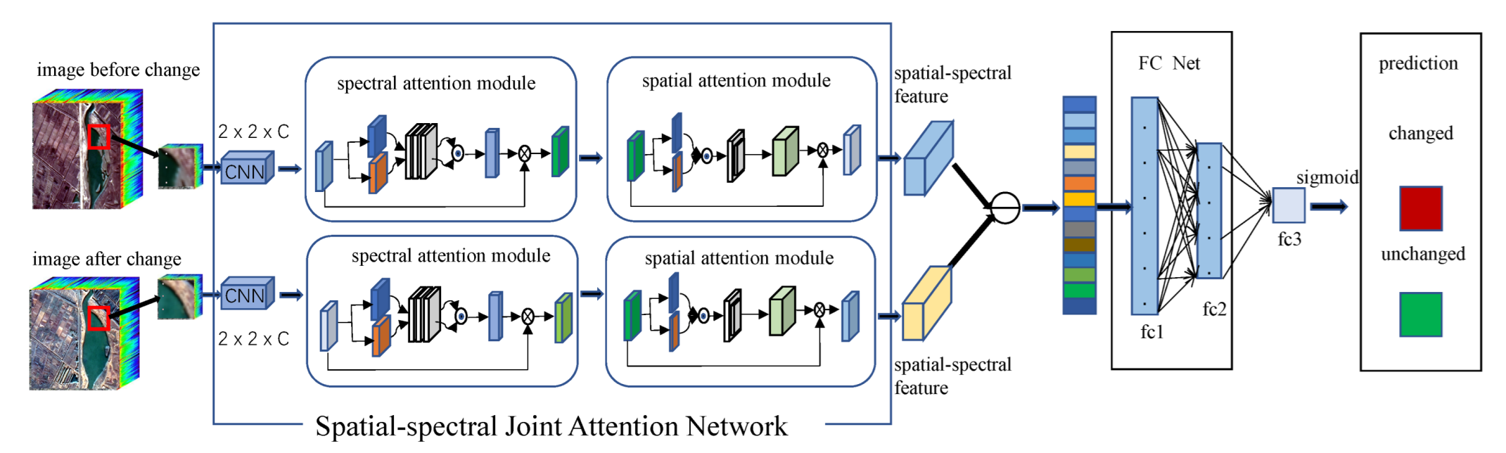
SJAN contains four parts: initial feature-extraction module, spectral-attention module, spatial-attention module, and discrimination module, as shown in Figure 1. The initial feature-extraction module uses the simplest CNN network. The network structure and relevant parameters of the initial feature-extraction module are shown in Table 1. The spatial-attention module and the spectral-attention module aim to optimize the learned initial features so that they can focus on the spatially critical changed regions and separability bands of the spectrum, which will be described in detail in the following section. The discrimination module first fuses the extracted spatial–spectral features, then explores the implicit information of the obtained features, and finally gives the change-detection result with the sigmoid function. Its network structure and relevant parameters are shown in Table 1.
First, the spatial–spectral features are extracted from the pairwise blocks at the moment and after a series of convolution and pooling operations, denoted as and , where H, W, and C represent the height, width, and number of channels, respectively. Second, the learned features and are fed to the spectral-attention module, respectively, to obtain the features based on spectral attention, denoted as and , which are obtained by multiplying the feature maps with the spectral-attention weights. Third, the features based on spectral attention and are fed to the spatial-attention module to obtain the spatial–spectral features, denoted as and . Finally, the differential information of the spatial–spectral features and is fed to the fully connected layers for classification to get the change-detection results.
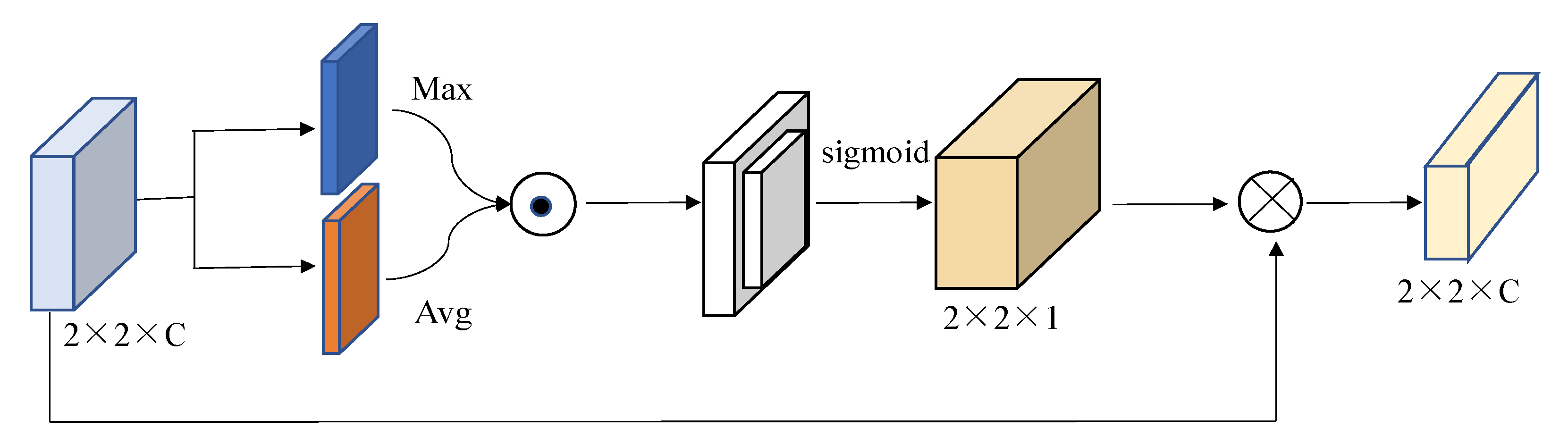
2.2.2. Spatial-Attention Module
The spatial-attention module consists of two arithmetic operations and one convolutional layer. It aims to obtain spatial-attention features of each channel. The structure of the spatial-attention module is shown in Figure 2. First, the mean and maximum values for the featured dimensions of the pairwise blocks are obtained to create two vectors, then the vectors are reduced to a vector. Second, the maximum value and the mean value will be dotted. The maximum and mean values of the feature dimensions are calculated to define the changed areas from different aspects, respectively. We perform a point multiplication operation which can obtain an attention matrix with higher weight differences than the concatenation operation, allowing us to better integrate the acquired data. Third, the data are normalized using the convolution and sigmoid function to obtain the spatial attention weights. Finally, the spatial attention weights and the input features are multiplied to obtain the spatial-attention features. The features obtained from the spatial-attention module are more discriminative because it focuses more on key changed regions in the spatial dimension.
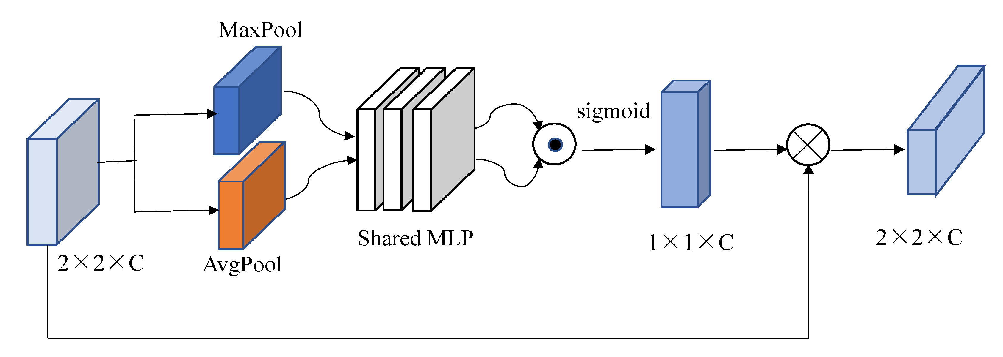
2.2.3. Spectral-Attention Module
The spectral-feature-extraction network under the attention mechanism can automatically determine the importance of different bands of pairwise blocks in complex scenes, which is useful for multispectral change-detection tasks. The spectral-attention module consists of two pooling layers and a shared MLP. It aims to explore which band is more effective for detecting the target. Figure 3 depicts the network architecture of the spectral-attention module. First, the features of the pairwise blocks are downscaled using global maximum pooling and global average pooling to create a vector (C is the number of channels). Second, they are fed into a shared MLP with two convolutions to ensure that the detailed information of pairwise blocks are acquired. Third, these learned features are dotted. Maximum pooling and average pooling focus on different aspects of the spectral information of the pairwise blocks, respectively, so that we perform a point multiplication operation instead of element-wise summation to make the gap between separability bands for different features as wide as possible. Then the sigmoid function is used to normalize the result, and the result after normalization is the spectral-attention-weight matrix based on the spectral-attention model. Finally, the channel-spectral-attention weights and the input features are multiplied to obtain the spectral-attention features. The features acquired from the spectral-attention module are more discriminative because it focuses more on the separability bands in the spectral dimension.
2.3. Loss Function
Spectral angle is a critical criterion for determining if two spectral vectors are similar, and most existing deep-learning-based change-detection methods do not take the spectral angle into consideration when calculating the similarity. Therefore, the loss function in this thesis is defined from both spectral magnitude and angle perspectives. The loss function of the proposed SJAN includes two terms: spectral amplitude terms and spectral angle term. The total loss function L is defined as follows:
where represents the loss of spectral amplitude. is the loss of the spectral angle of multispectral images.
contains two parts: and , and is defined as follows:
where the parameters , , and are the penalty parameters of the loss functions , , and . The optimal values of three parameters are discussed in the Section 4.1.
is calculated from the contrast loss function. This loss function is a common measure of the similarity of multispectral images. It considers the similarity of multispectral images from the spectral amplitude, constraining the distance of similar image block pairs and expanding the space of dissimilar image block pairs. It is defined as follows:
where the value of l represents the label information of the input pairwise patch. indicates that the patch pair is dissimilar, while means that the patch pair is similar. m represents the margin for dissimilar pairs. In our experiment, m is set to . What is more, d represents the distance of two input patches. It can be seen that the distance of the dissimilar pairs between 0 and m is only considered. If and d is greater than the margin, the loss is regarded as 0.
is calculated by cross-entropy loss. The cross-entropy loss function for the extracted spatial–spectral features aims to make the model predictions closer to the labeled values. It is defined as follows:
where the value of is 0 or 1, which means the label of information of input pair. equals 1 means that the input image block pair is changed. represents the probability that the input image is a changed sample pair.
is a more comprehensive similarity metric that multiplies the spectral cosine and the Euclidean distance directly. To make the spectral cosine have the same principle as the Euclidean distance, we use the formula so that a smaller value of the formula represents a closer proximity of similar image blocks. is defined as follows:
where , represent the spectral values of the ith band.
2.4. Training Process
As shown in Figure 1, SJAN is trained in a supervised manner. The data will be pre-processed and then trained in batches. The difference after fully connected layers characterizes the input of cross-entropy loss; the contrast loss function and spectral angle similarity are characterized by the two-stream network after the attention mechanism module. Back propagation is used to update the network weights. Moreover, the weight updating strategy uses the Adam optimization algorithm. Through multiple types of training, the optimal model is obtained. Finally, the test data are fed directly to the obtained optimal model to achieve the change-detection map.
The complete end-to-end steps of the proposed SJAN are described in Algorithm 1.
| Algorithm 1 Framework of SJAN. |
| Input: |
|
|
| Output: |
|
3. Results
3.1. Datasets
The effectiveness of the proposed SJAN is validated on three datasets, and the three multispectral datasets are described in detail as follows.
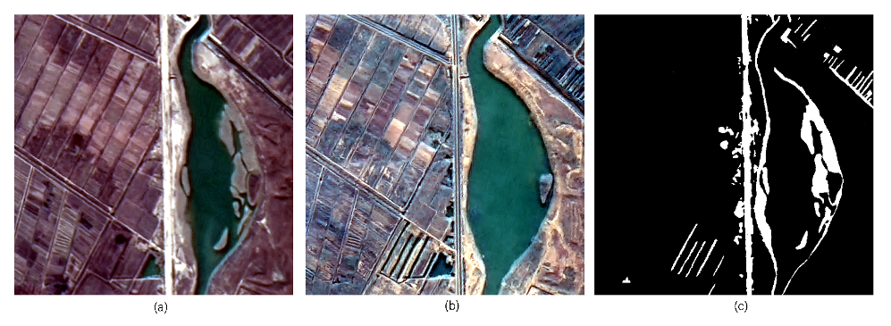
We used the Minfeng, Hongqi Canal, and Weihe river datasets acquired by the GF-1 satellite sensor as our dataset. Each dataset contains two multispectral images with a spatial resolution of 2 m. The two multispectral images have different times and each image contains four bands: red, green, blue, and near-infrared bands. Figure 4 shows the images of the Hongqi Cancal dataset. The Hongqi Cancal dataset with the image size of , located in West Kowloon Village, Kenli County, Dongying City, Shandong Province, was acquired with the GF-1 satellite on 9 December 2013 and 16 October 2015. Figure 5 shows the image of the Minfeng dataset with the image size of , taken in Kenli County, Dongying City, Shandong Province. The acquisition time is the same as Hongqi Cancal. Figure 6 shows the Weihe river dataset with an image size of , located in Madong Village, Xi’an City, Shaanxi Province, acquired on 19 August 2013 and 29 August 2015, respectively.
3.2. Evaluation Criteria
The proposed SJAN is quantitatively analyzed to demonstrate its robustness and effectiveness. Three evaluation metrics are used to analyze it, overall accuracy , Kappa coefficient, and (area under the ROC zone line) value.
Firstly, the overall accuracy is used for evaluation, and the value of is within , closer to 1 means better detection performance.
where refers to true position, stands for true negative, stands for false positive and represents false negative.
Secondly, the accuracy of the classification is measured using the kappa coefficient, which is within and is usually within , with closer to 1 meaning a better performance. The formula for calculating the kappa coefficient based on the confusion matrix is defined as follows:
Finally, the numerical accuracy measure is provided using the . The larger the value of the , the better the classification effect of the classifier. With as the horizontal axis and as the vertical axis, the curve is plotted and the area under the curve is the value, where represents the true positive rate and FPR represents the false positive rate, both of which are calculated as follows:
3.3. Competitors
The proposed SJAN is compared with the following methods:
The main contributions of our proposed SJAN method are as follows:
- (1)
- CVA [31] is a typically unsupervised change-detection method. Difference operations are performed on the images from two temporal images to identify the changed areas.
- (2)
- IRMAD [34] assigns larger weights to the pixels that have not changed, and after several iterations, the weights of the pixel points are compared with the threshold value to determine whether they have changed. IR-MAD is better than MAD in identifying significant changes, and this method is widely used in multivariate change detection.
- (3)
- SCCN [37] is a symmetric network, which includes a convolutional layer and several coupling layers. The input images are connected to each side of the network and are transformed into a feature space. The distances of the feature pairs are calculated to generate the difference map.
- (4)
- SSJLN [40] considers both spectral and spatial information and deeply explores the implicit information of the fused features. SSJLN is very good at improving change-detection performance.
- (5)
- STA [27] designs a new CD based on the self-attention module to simulate a spatial–temporal relationship. The self-attention module can calculate the attention weights between any two pixels at different times and locations, which can generate more discriminative features.
- (6)
- DSAMNet [52] includes a CBAM-integrated metric module that learns a change map directly through the feature extractor and an auxiliary deep-supervision module that generates change maps with more spatial information.
3.4. Performance Analysis
First, we conduct a comparison of the training time and the number of parameters of the SJAN method with other deep-learning-based methods to measure the performance of the proposed network. Due to the addition of the attention module, the proposed SJAN method has a higher number of parameters and training time compared to SCCN and SSJLN, as shown in Table 2. Compared with STA and DSAMNet methods based on the attention mechanism, our proposed SJAN method has fewer parameters and less training time.
Second, we compare the experimental results of SJAN with other existing change-detection methods from both qualitative and quantitative aspects.
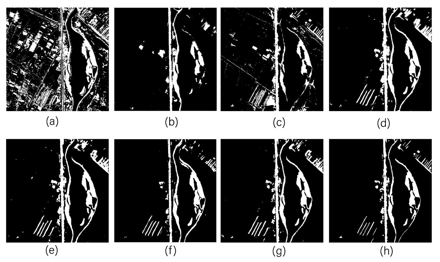
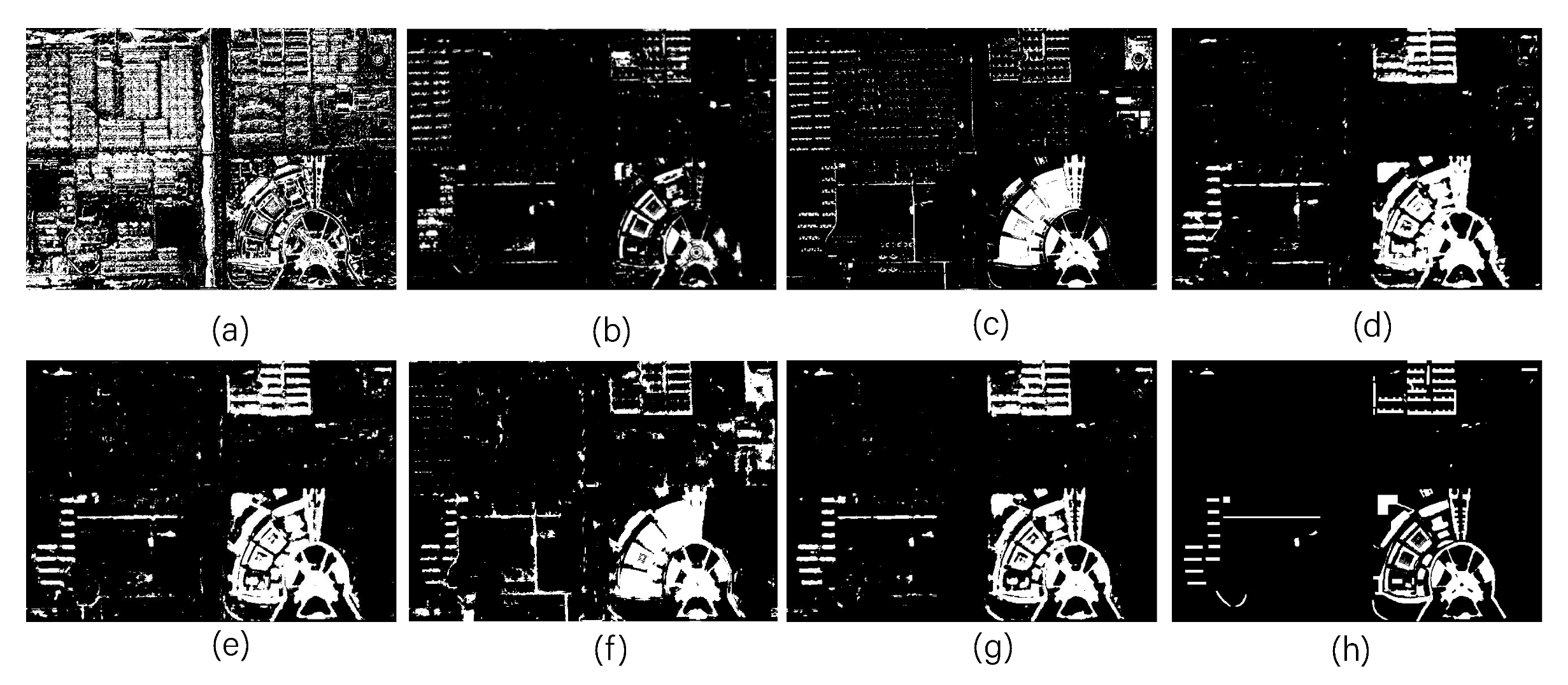
The qualitative performances of comparative change-detection methods on the Hongqi Canal, Minfeng, and Weihe river datasets are visually shown in Figure 7, Figure 8 and Figure 9, respectively. We can clearly see that the CVA method has a large false-alarm rate, detecting changes in almost the entire image, which is not the case in reality. IRMAD detects many changed pixels as unchanged pixels by mistake and has a high omission rate. Traditional change-detection methods rely on manual features that are costly in terms of time and need be designed by professionals. Deep learning can extract more abstract and hierarchical features. Hence, deep-learning-based change-detection methods are attracting more and more attention.
SCCN is an unsupervised deep-learning-based change-detection technique that does not consider the label information. Moreover, SCCN does not take the detection of subtle changes and the joint distribution of changed and unchanged pixels into account. Therefore, we can see that the detection results of SCCN include many white-noise spots. SSJLN learns the semantic difference between changed pixels and unchanged pixels by extracting spatial–spectral joint features. From (c) and (d) of Figure 7, Figure 8 and Figure 9, it is clear to see that the number of unchanged pixels incorrectly detected by SSJLN as changed pixels is significantly reduced.
The STA method proposed in the last two years applies the attention module to the change detection, and it can be found that the attention module has a positive effect on the change-detection task. However, when extracting spatial–spectral features, the STA method does not take the spectral angle loss into account. SJAN performs the similarity measures from both the spectral angle and the spectral magnitude, which can exploit more discriminative information. Moreover, SJAN uses a fusion strategy of point multiplication to obtain attention weights. It can be observed that SJAN achieves the best results.
The DSAMNet method employs a deep supervised network and an attention mechanism to extract more discriminative features. However, it can be seen from Figure 7, Figure 8 and Figure 9 that the detection performance of DSAMNet on the Hongqi, Mingfeng, and Weihe datasets is not very good. Many changed pixels on the Weihe dataset are misclassified as unchanged pixels, as shown in Figure 9. In contrast, many unchanged pixels on the Minfeng dataset are detected as changed pixels by mistake, as shown in Figure 8. DSAMNet is more suitable for very high-resolution images such as 0.5 m aerial images that contain more spatial information. The spatial resolution of Hongqi, Mingfeng and Weihe datasets is 2 m. It can be concluded that SJAN is more suitable than DSAMNet for the change-detection task on the GF-1 dataset.
As shown in Table 3, we calculated , , and values to quantitatively analyze the effect of the SJAN method. The , , and values for the Hongqi dataset are 97.72, 87.75, and 97.70, respectively. The , , and values for the Minfeng dataset are 95.96, 77.15, and 97.41, respectively. The , , and values for the Weihe dataset are 98.89, 97.08, and 98.45, respectively. It can be clearly seen that SJAN has the best detection accuracy among these methods, which is consistent with the results of the qualitative analysis based on the changed detection maps. Therefore, it can be concluded that the proposed SJAN method has better performance than other comparison methods.
4. Discussion
4.1. Parameter Settings
This subsection describes the settings of the relevant parameters of the network model, including the convolution, the kernel size for pooling, and the activation function used.
First, the parameters of SJAN are shown in Table 1. Specifically, the Siamese network structure includes two convolutional layers (conv1 and conv2), one layer of maximum pooling (pool1) and two layers of convolution (conv3 and conv4), one layer of maximum pooling (pool2) to ensure that the essential features of the images can be fully extracted. The kernel size of the convolution is and the kernel size of pooling is . The network structure of spectral- and spatial-attention modules has been described in detail and will not be repeated. The fully connected net is designed as two layers, each with dimensions 256, 128, and finally the fully connected layer with output dimension 1 is classified using the sigmoid function. What is more, the input and output dimensions are . is the number of bands, where the number of bands is 4 for GF-1.
Second, the patch size can have an effect on the test results, so we discuss it in details.
Effect of Patch
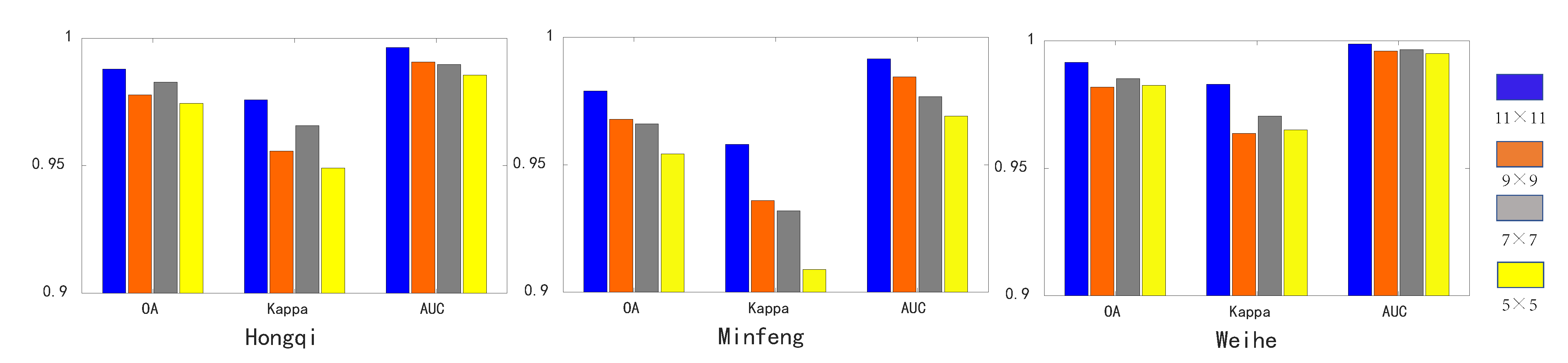
Image blocks contain not only the spectral information of the pixel to be detected, but also the spectral information of its neighboring pixels. Therefore, we use image blocks as the basic processing unit. The size of the image block n greatly affects the accuracy of change detection. The larger the image block, the more detailed the spectral information it contains. However, at the same time, the image block size is chosen as too large, its local key information will be more disturbed. The exponential increase in data volume will also put very high pressure on the training. In our experiments, we set the image block size to 5, 7, 9, and 11, respectively. The experimental results are shown in Figure 10, where blue, orange, gray, and yellow represent image block sizes of 11, 9, 7, and 5, respectively.
It is obvious from Figure 10 that the detection accuracy is worst when n is 5, and the values of , , and are the best when n is 11. What is more, when n is larger than 11, the training data is very large and the training time cost increases exponentially. Therefore, we select the patch size as 11.
Third, the other relevant experimental parameters such as training-data division, batch size, and learning rate will be introduced.
We select 70 percent of the changed samples and an equal number of unchanged samples to construct the training set. The training and validation data in the training set are further divided into 7:3. In the training phase, a batching strategy is used and the number of samples for each batch is 32. The initial learning rate is set to using the Adam optimizer optimization algorithm. During the experiment, the learning rate is continuously decreased according to the strategy, and after 20 iterations, the respective optimal experimental results are obtained on different datasets. The results on the validation set are shown in Table 4. We can see the results of the validation set are a bit better than those on the testing dataset shown in Table 3. This is because the data distribution of the validated set is more similar to that of the training set than that of the testing set.
Moreover, we test the effect of the penalty parameters of the loss function on the change-detection performance. As shown in Figure 11, some of the parameter combinations are listed. Status-a represents that , , and are set to 1, 1, and 1. Status-b represents those three penalty parameters are set to , , and , and the proposed SJAN achieves the best detection on Weihe and Minfeng datasets with these parameter settings. Status-c represents those three penalty parameters are set to , , and . Status-d represents those three penalty parameters are set to , , and 1, and the Hongqi dataset has better performance results with these parameter settings. In our experiment, the parameters of , and are set to , , and on the Hongqi dataset, and , , and on Minfeng and Weihe River datasets.
4.2. Comparison with CBAM
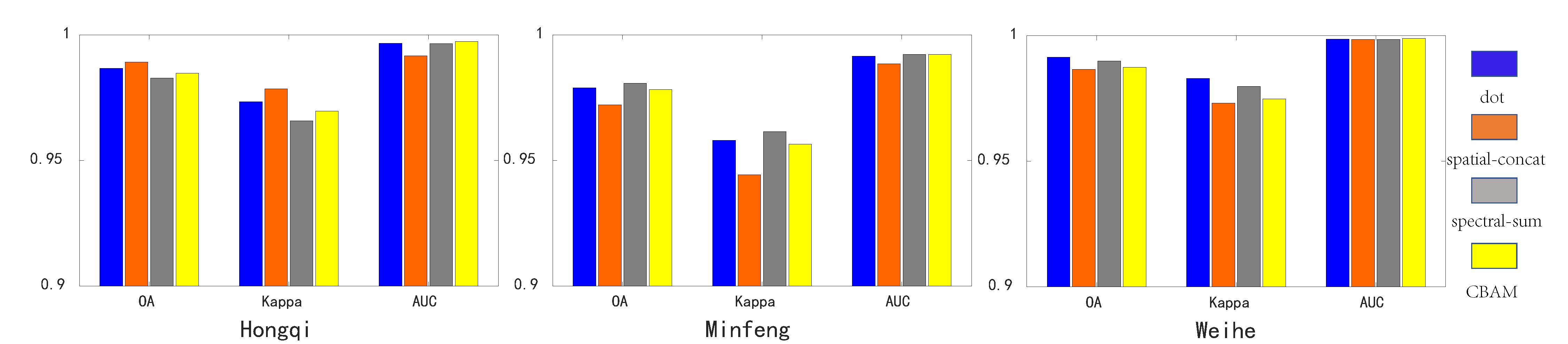
In this section, we will discuss the difference between the point multiplication operation in the proposed spatial–spectral-attention module and the element-wise summation and concatenation operations of the original CBAM.
As shown in Figure 12, blue indicates the result of using point multiplication operations in both the spectral-attention module and the spatial-attention module, denoted as dots. Orange indicates the result of using a point-multiplication operation between MLP outputs instead of an element-wise-summation operation in the spectral-attention module, denoted as spatial-concat. Gray indicates the result of using a point multiplication operation between Maxpooling and Avgpooling instead of the concatenation operation in the spatial-attention module, denoted as spectral-sum. Yellow represents the results of the original CBAM method. It can be seen that using point multiplication instead of element-wise summation in the spectral-attention module achieves better detection performance on the Hongqi dataset, and using point multiplication instead of concatenation in the spatial-attention module can gain better detection accuracy on the Minfeng dataset. What is more, using the point multiplication operation on the Weihe dataset yields better results in both the spectral and spatial-attention modules. As a result, the point multiplication operation is chosen in the spectral and spatial modules to explore more similar information.
4.3. Ablation Experiment
• Effect of the spectral- and spatial-attention modules
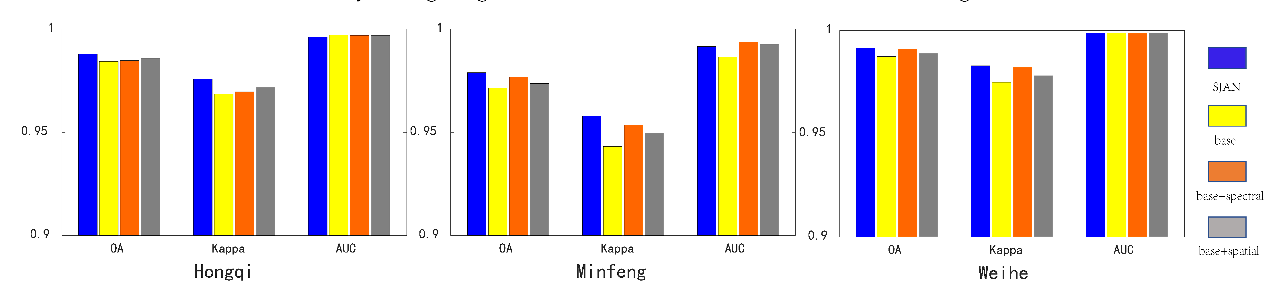
The proposed SJAN includes the spatial-attention module and a spectral-attention module. When extracting spatial–spectral features, the spatial-attention module focuses on feature extraction of spatially key regions and the spectral-attention module can identify separable bands of different land covers. This section conducts comparative experiments to verify the impact of the spectral- and spatial-attention modules on the detection accuracy. Figure 13 shows the ablation experiment of the spectral-attention module and the spatial-attention module in detail. Blue indicates the feature-extraction method based on SJAN, and yellow indicates the feature-extraction method with spatial- and spectral-attention modules removed, denoted as base network. Orange indicates the feature-extraction method with the spectral-attention module only, denoted as base + spectral. Gray indicates the feature-extraction method with the spatial-attention module only, denoted as base + spatial. Both the base + spectral method and the base + spatial method achieve better detection accuracy than the base method, which proves the effectiveness of the spatial- and spectral-attention modules. What is more, it can be seen that Hongqi Cancal, Minfeng, and Weihe River datasets based on SJAN have higher values of and than those of other methods, and the values of SJAN are not significantly different from other comparison methods. The results of the ablation experiment show that the spectral-attention module focusing on separable bands in the spectral dimension and the spatial-attention module focusing on key change regions have some beneficial effects on the change-detection task.
• Effect of
This section experimentally verifies the effect of the loss function with the spectral angular cosine-Euclidean distance on the detection accuracy of different datasets.
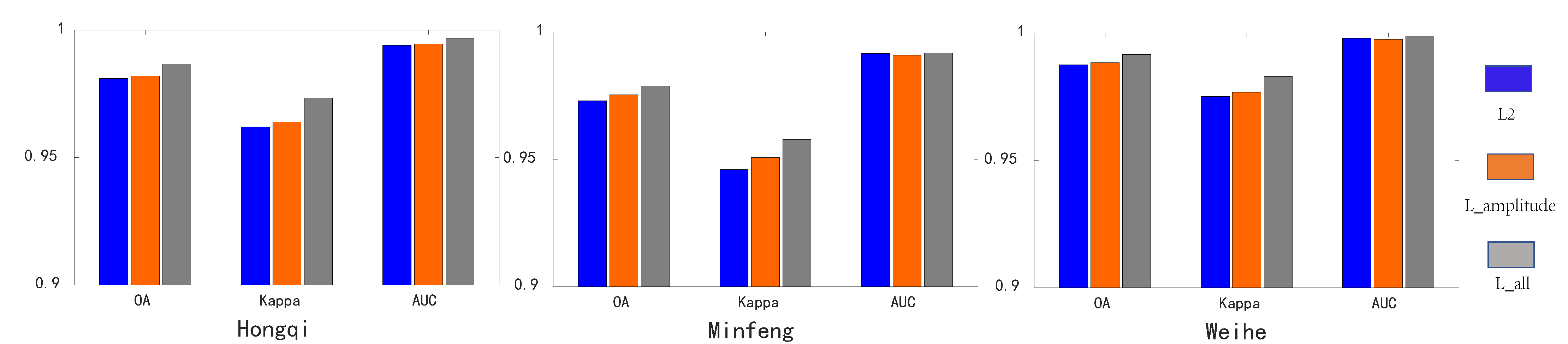
The proposed loss function not only considers the similarity measure of spectral magnitude, but also considers the similarity measure of spectral angle. The contrast loss function and cross-entropy loss are used from the magnitude dimension. The spectral angular cosine-Euclidean distance is used to explore the spectral angular features of the images from the spectral angle dimension. The , , and values of the detection results on different datasets are shown in Figure 14. Blue indicates the results of the change detection using loss function, denoted as . Orange indicates the results of loss function that includes both and , denoted as . Gray indicates the effect of the total loss function that includes and on the detection results, denoted as . It can be clearly seen that , which has accurate detection results for the more intricate details, has a positive effect on the change-detection task.
5. Conclusions
A multispectral-image-change-detection method based on the spatial–spectral joint attention network is proposed. The spatial-attention module and spectral-attention module are simultaneously incorporated into the Siamese network to extract more effective and discriminative spatial–spectral features. The spectral-attention module is used to explore the separability bands and the spatial-attention module is used to capture spatially critical regions of variation. In addition, a new loss function is proposed to consider the loss of spatial–spectral features from the spectrum amplitude and angle perspectives. The proposed SJAN method in this paper is validated on three real datasets to verify its effectiveness. The experimental results show that SJAN has better detection performance compared with other existing methods.
However, our proposed joint spatial–spectral attention network does not consider the correlation between images at different moments when extracting features. The correlation between images at different moments has an impact on the change-detection performance. In the future, we will improve the attention module using the cross-attention mechanism to obtain the correlation of remote-sensing images at different moments. In addition, we will further address the issue of sample imbalance in future work.
Author Contributions
W.Z., Q.Z., S.L., X.P. and X.L. made contributions to proposing the method, doing the experiments and analyzing the result. W.Z., Q.Z., S.L., X.P. and X.L. are involved in the preparation and revision of the manuscript. All authors have read and agreed to the published version of the manuscript.
Funding
This work was supported in part by the Shaanxi Provincial Department of Education 2020 Scientific Research Plan under Grant 20JK0913, in part by the National Natural Science Foundation of China under Grant 62001378, in part by the Shaanxi Province Network Data Analysis and Intelligent Processing Key Laboratory Open Fund under Grant XUPT-KLND(201902), and by a special project for the construction of key disciplines in general higher education institutions in Shaanxi Province.
Conflicts of Interest
The authors declare no conflict of interest.
References
- Haque, M.A.; Shishir, S.; Mazumder, A.; Iqbal, M. Change detection of Jamuna River and its impact on the local settlements. Phys. Geogr. 2022, 1–21. [Google Scholar] [CrossRef]
- Pasang, S.; Norbu, R.; Timsina, S.; Wangchuk, T.; Kubíček, P. Normalized difference vegetation index analysis of forest cover change detection in Paro Dzongkhag, Bhutan. In Computers in Earth and Environmental Sciences; Elsevier: Amsterdam, The Netherlands, 2022; pp. 417–425. [Google Scholar]
- Hajarian, M.H.; Atarchi, S.; Hamzeh, S. Monitoring seasonal changes of Meighan wetland using SAR, thermal and optical remote sensing data. Phys. Geogr. Res. Q. 2021, 53, 365–380. [Google Scholar]
- Hasanlou, M.; Seydi, S.T. Use of multispectral and hyperspectral satellite imagery for monitoring waterbodies and wetlands. In Southern Iraq’s Marshes; Springer: Berlin/Heidelberg, Germany, 2021; pp. 155–181. [Google Scholar]
- Guo, R.; Xiao, P.; Zhang, X.; Liu, H. Updating land cover map based on change detection of high-resolution remote sensing images. J. Appl. Remote. Sens. 2021, 15, 044507. [Google Scholar] [CrossRef]
- Di Francesco, S.; Casadei, S.; Di Mella, I.; Giannone, F. The Role of Small Reservoirs in a Water Scarcity Scenario: A Computational Approach. Water Resour. Manag. 2022, 36, 875–889. [Google Scholar] [CrossRef]
- Li, J.; Peng, B.; Wei, Y.; Ye, H. Accurate extraction of surface water in complex environment based on Google Earth Engine and Sentinel-2. PLoS ONE 2021, 16, e0253209. [Google Scholar] [CrossRef]
- Lynch, P.; Blesius, L.; Hines, E. Classification of urban area using multispectral indices for urban planning. Remote Sens. 2020, 12, 2503. [Google Scholar] [CrossRef]
- Huang, B.; Zhao, B.; Song, Y. Urban land-use mapping using a deep convolutional neural network with high spatial resolution multispectral remote sensing imagery. Remote Sens. Environ. 2018, 214, 73–86. [Google Scholar] [CrossRef]
- Yang, C.; Zhao, S. Urban vertical profiles of three most urbanized Chinese cities and the spatial coupling with horizontal urban expansion. Land Use Policy 2022, 113, 105919. [Google Scholar] [CrossRef]
- Aamir, M.; Ali, T.; Irfan, M.; Shaf, A.; Azam, M.Z.; Glowacz, A.; Brumercik, F.; Glowacz, W.; Alqhtani, S.; Rahman, S. Natural disasters intensity analysis and classification based on multispectral images using multi-layered deep convolutional neural network. Sensors 2021, 21, 2648. [Google Scholar] [CrossRef]
- Jun, L.; Shao-qing, L.; Yan-rong, L.; Rong-rong, Q.; Tao-ran, Z.; Qiang, Y.; Ling-tong, D. Evaluation and Modifying of Multispectral Drought Severity Index. Spectrosc. Spectr. Anal. 2020, 40, 3522. [Google Scholar]
- Peng, B.; Meng, Z.; Huang, Q.; Wang, C. Patch similarity convolutional neural network for urban flood extent mapping using bi-temporal satellite multispectral imagery. Remote Sens. 2019, 11, 2492. [Google Scholar] [CrossRef] [Green Version]
- Afaq, Y.; Manocha, A. Analysis on change detection techniques for remote sensing applications: A review. Ecol. Inform. 2021, 63, 101310. [Google Scholar] [CrossRef]
- Gong, M.; Zhan, T.; Zhang, P.; Miao, Q. Superpixel-based difference representation learning for change detection in multispectral remote sensing images. IEEE Trans. Geosci. Remote Sens. 2017, 55, 2658–2673. [Google Scholar] [CrossRef]
- Geng, J.; Wang, H.; Fan, J.; Ma, X. Change detection of SAR images based on supervised contractive autoencoders and fuzzy clustering. In Proceedings of the 2017 International Workshop on Remote Sensing with Intelligent Processing (RSIP), Shanghai, China, 18–21 May 2017; pp. 1–3. [Google Scholar]
- Su, L.; Gong, M.; Zhang, P.; Zhang, M.; Liu, J.; Yang, H. Deep learning and mapping based ternary change detection for information unbalanced images. Pattern Recognit. 2017, 66, 213–228. [Google Scholar] [CrossRef]
- Gao, F.; Dong, J.; Li, B.; Xu, Q. Automatic change detection in synthetic aperture radar images based on PCANet. IEEE Geosci. Remote Sens. Lett. 2016, 13, 1792–1796. [Google Scholar] [CrossRef]
- Zhan, T.; Song, B.; Sun, L.; Jia, X.; Wan, M.; Yang, G.; Wu, Z. TDSSC: A Three-Directions Spectral–Spatial Convolution Neural Network for Hyperspectral Image Change Detection. IEEE J. Sel. Top. Appl. Earth Obs. Remote Sens. 2020, 14, 377–388. [Google Scholar] [CrossRef]
- Zhang, Y.; Liu, G.; Yuan, Y. A novel unsupervised change detection approach based on spectral transformation for multispectral images. In Proceedings of the 2020 IEEE International Conference on Image Processing (ICIP), Abu Dhabi, United Arab Emirates, 25–28 October 2020; pp. 51–55. [Google Scholar]
- Liu, Y.; Pang, C.; Zhan, Z.; Zhang, X.; Yang, X. Building change detection for remote sensing images using a dual-task constrained deep siamese convolutional network model. IEEE Geosci. Remote Sens. Lett. 2020, 18, 811–815. [Google Scholar] [CrossRef]
- Zhan, T.; Gong, M.; Jiang, X.; Zhang, M. Unsupervised scale-driven change detection with deep spatial–spectral features for VHR images. IEEE Trans. Geosci. Remote Sens. 2020, 58, 5653–5665. [Google Scholar] [CrossRef]
- Liu, G.; Yuan, Y.; Zhang, Y.; Dong, Y.; Li, X. Style transformation-based spatial–spectral feature learning for unsupervised change detection. IEEE Trans. Geosci. Remote Sens. 2020, 60, 5401515. [Google Scholar] [CrossRef]
- Lei, T.; Wang, J.; Ning, H.; Wang, X.; Xue, D.; Wang, Q.; Nandi, A.K. Difference Enhancement and Spatial–Spectral Nonlocal Network for Change Detection in VHR Remote Sensing Images. IEEE Trans. Geosci. Remote Sens. 2021, 60, 1–13. [Google Scholar] [CrossRef]
- Wang, D.; Chen, X.; Jiang, M.; Du, S.; Xu, B.; Wang, J. ADS-Net: An Attention-Based deeply supervised network for remote sensing image change detection. Int. J. Appl. Earth Obs. Geoinf. 2021, 101, 102348. [Google Scholar]
- Chen, J.; Yuan, Z.; Peng, J.; Chen, L.; Huang, H.; Zhu, J.; Liu, Y.; Li, H. DASNet: Dual attentive fully convolutional siamese networks for change detection in high-resolution satellite images. IEEE J. Sel. Top. Appl. Earth Obs. Remote Sens. 2020, 14, 1194–1206. [Google Scholar] [CrossRef]
- Chen, H.; Shi, Z. A spatial–temporal attention-based method and a new dataset for remote sensing image change detection. Remote Sens. 2020, 12, 1662. [Google Scholar] [CrossRef]
- Chen, L.; Zhang, D.; Li, P.; Lv, P. Change detection of remote sensing images based on attention mechanism. Comput. Intell. Neurosci. 2020, 2020, 6430627. [Google Scholar] [CrossRef]
- Ma, W.; Zhao, J.; Zhu, H.; Shen, J.; Jiao, L.; Wu, Y.; Hou, B. A spatial-channel collaborative attention network for enhancement of multiresolution classification. Remote Sens. 2020, 13, 106. [Google Scholar] [CrossRef]
- Chen, S.; Yang, K.; Stiefelhagen, R. DR-TANet: Dynamic Receptive Temporal Attention Network for Street Scene Change Detection. In Proceedings of the 2021 IEEE Intelligent Vehicles Symposium (IV), Nagoya, Japan, 11–17 July 2021. [Google Scholar]
- Bovolo, F.; Bruzzone, L. A theoretical framework for unsupervised change detection based on change vector analysis in the polar domain. IEEE Trans. Geosci. Remote Sens. 2006, 45, 218–236. [Google Scholar] [CrossRef] [Green Version]
- Deng, J.; Wang, K.; Deng, Y.; Qi, G. PCA-based land-use change detection and analysis using multitemporal and multisensor satellite data. Int. J. Remote Sens. 2008, 29, 4823–4838. [Google Scholar] [CrossRef]
- Nielsen, A.A.; Conradsen, K.; Simpson, J.J. Multivariate alteration detection (MAD) and MAF postprocessing in multispectral, bitemporal image data: New approaches to change detection studies. Remote Sens. Environ. 1998, 64, 1–19. [Google Scholar] [CrossRef] [Green Version]
- Canty, M.J.; Nielsen, A.A. Automatic radiometric normalization of multitemporal satellite imagery with the iteratively re-weighted MAD transformation. Remote Sens. Environ. 2008, 112, 1025–1036. [Google Scholar] [CrossRef] [Green Version]
- Radhika, K.; Varadarajan, S. A neural network based classification of satellite images for change detection applications. Cogent Eng. 2018, 5, 1484587. [Google Scholar] [CrossRef]
- Vignesh, T.; Thyagharajan, K.; Murugan, D.; Sakthivel, M.; Pushparaj, S. A novel multiple unsupervised algorithm for land use/land cover classification. Indian J. Sci. Technol. 2016, 9, 1–12. [Google Scholar] [CrossRef] [Green Version]
- Liu, J.; Gong, M.; Qin, K.; Zhang, P. A deep convolutional coupling network for change detection based on heterogeneous optical and radar images. IEEE Trans. Neural Netw. Learn. Syst. 2016, 29, 545–559. [Google Scholar] [CrossRef]
- Zhan, Y.; Fu, K.; Yan, M.; Sun, X.; Wang, H.; Qiu, X. Change detection based on deep siamese convolutional network for optical aerial images. IEEE Geosci. Remote Sens. Lett. 2017, 14, 1845–1849. [Google Scholar] [CrossRef]
- Mou, L.; Bruzzone, L.; Zhu, X.X. Learning spectral–spatial–temporal features via a recurrent convolutional neural network for change detection in multispectral imagery. IEEE Trans. Geosci. Remote Sens. 2018, 57, 924–935. [Google Scholar] [CrossRef] [Green Version]
- Zhang, W.; Lu, X. The Spectral-Spatial Joint Learning for Change Detection in Multispectral Imagery. Remote Sensing 2019, 11, 240. [Google Scholar] [CrossRef] [Green Version]
- Vaswani, A.; Shazeer, N.; Parmar, N.; Uszkoreit, J.; Jones, L.; Gomez, A.N.; Kaiser, Ł.; Polosukhin, I. Attention is all you need. Adv. Neural Inf. Process. Syst. 2017, 30, 3–6. [Google Scholar]
- Ramachandran, P.; Parmar, N.; Vaswani, A.; Bello, I.; Levskaya, A.; Shlens, J. Stand-alone self-attention in vision models. Adv. Neural Inf. Process. Syst. 2019, 32, 3–5. [Google Scholar]
- Cai, W.; Liu, B.; Wei, Z.; Li, M.; Kan, J. TARDB-Net: Triple-attention guided residual dense and BiLSTM networks for hyperspectral image classification. Multimed. Tools Appl. 2021, 80, 11291–11312. [Google Scholar] [CrossRef]
- Yu, C.; Han, R.; Song, M.; Liu, C.; Chang, C.I. Feedback attention-based dense CNN for hyperspectral image classification. IEEE Trans. Geosci. Remote Sens. 2021, 60, 1–16. [Google Scholar] [CrossRef]
- Shi, C.; Liao, D.; Zhang, T.; Wang, L. Hyperspectral Image Classification Based on 3D Coordination Attention Mechanism Network. Remote Sens. 2022, 14, 608. [Google Scholar] [CrossRef]
- Peng, C.; Tian, T.; Chen, C.; Guo, X.; Ma, J. Bilateral attention decoder: A lightweight decoder for real-time semantic segmentation. Neural Netw. 2021, 137, 188–199. [Google Scholar] [CrossRef]
- Fu, J.; Zheng, H.; Mei, T. Look closer to see better: Recurrent attention convolutional neural network for fine-grained image recognition. In Proceedings of the IEEE Conference on Computer Vision and Pattern Recognition, Honolulu, HI, USA, 21–26 July 2017; pp. 4438–4446. [Google Scholar]
- Hu, J.; Shen, L.; Sun, G. Squeeze-and-excitation networks. IEEE Trans. Pattern Anal. Mach. Intell. 2018, 42, 7132–7141. [Google Scholar]
- Woo, S.; Park, J.; Lee, J.Y.; Kweon, I.S. Cbam: Convolutional block attention module. In Proceedings of the European Conference on Computer Vision (ECCV), Munich, Germany, 8–14 September 2018; pp. 3–19. [Google Scholar]
- Misra, D.; Nalamada, T.; Arasanipalai, A.U.; Hou, Q. Rotate to attend: Convolutional triplet attention module. In Proceedings of the IEEE/CVF Winter Conference on Applications of Computer Vision, Waikoloa, HI, USA, 3–8 January 2021; pp. 3139–3148. [Google Scholar]
- Rahman, F.; Vasu, B.; Van Cor, J.; Kerekes, J.; Savakis, A. Siamese network with multi-level features for patch-based change detection in satellite imagery. In Proceedings of the 2018 IEEE Global Conference on Signal and Information Processing (GlobalSIP), Anaheim, CA, USA, 26–29 November 2018; pp. 958–962. [Google Scholar]
- Shi, Q.; Liu, M.; Li, S.; Liu, X.; Wang, F.; Zhang, L. A deeply supervised attention metric-based network and an open aerial image dataset for remote sensing change detection. IEEE Trans. Geosci. Remote Sens. 2021, 60, 1–16. [Google Scholar] [CrossRef]
Figure 1.
Spatial–spectral joint attention network.

Figure 2.
Spatial-Attention Module.

Figure 3.
Spectral Attention Module.

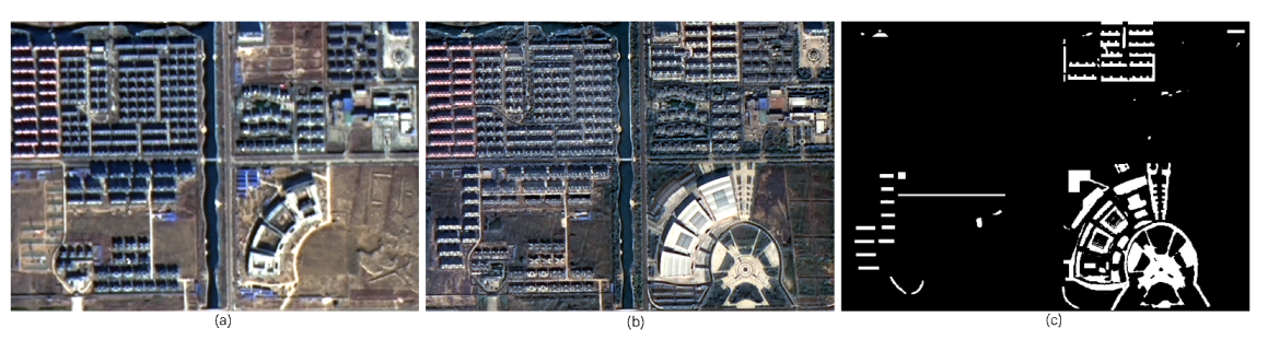
Figure 4.
Multispectral images and reference image of Hongqi Cancal dataset. (a) Image acquired on 9 December 2013. (b) Image acquired on 16 October 2015. (c) Reference image.
Figure 4.
Multispectral images and reference image of Hongqi Cancal dataset. (a) Image acquired on 9 December 2013. (b) Image acquired on 16 October 2015. (c) Reference image.

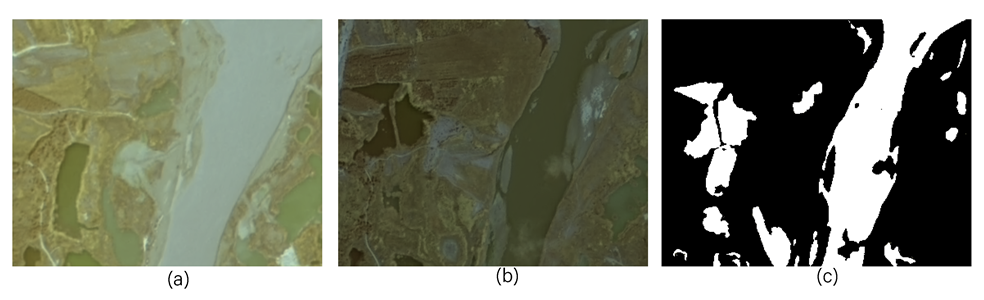
Figure 5.
Multispectral images and reference image of Minfeng dataset. (a) Image acquired on 9 December 2013. (b) Image acquired on 16 October 2015. (c) Reference image.
Figure 5.
Multispectral images and reference image of Minfeng dataset. (a) Image acquired on 9 December 2013. (b) Image acquired on 16 October 2015. (c) Reference image.

Figure 6.
Multispectral images and reference image of Weihe river dataset. (a) Image acquired on 19 August 2013. (b) Image acquired on 29 August 2015. (c) Reference image.
Figure 6.
Multispectral images and reference image of Weihe river dataset. (a) Image acquired on 19 August 2013. (b) Image acquired on 29 August 2015. (c) Reference image.

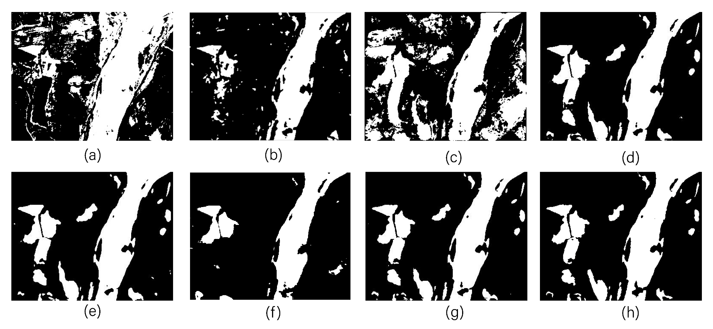
Figure 7.
Binary change maps of Hongqi Canal dataset. (a) CVA. (b) IRMAD. (c) SCCN. (d) SSJLN. (e) STA. (f) DSAMNet. (g) SJAN. (h) Ground truth. The unchanged samples are black and changed samples are white.
Figure 7.
Binary change maps of Hongqi Canal dataset. (a) CVA. (b) IRMAD. (c) SCCN. (d) SSJLN. (e) STA. (f) DSAMNet. (g) SJAN. (h) Ground truth. The unchanged samples are black and changed samples are white.

Figure 8.
Binary change maps of Minfeng dataset. (a) CVA. (b) IRMAD. (c) SCCN. (d) SSJLN. (e) STA. (f) DSAMNet. (g) SJAN. (h) Ground truth. The unchanged samples are black and changed samples are white.
Figure 8.
Binary change maps of Minfeng dataset. (a) CVA. (b) IRMAD. (c) SCCN. (d) SSJLN. (e) STA. (f) DSAMNet. (g) SJAN. (h) Ground truth. The unchanged samples are black and changed samples are white.

Figure 9.
Binary change maps of Weihe River dataset. (a) CVA. (b) IRMAD. (c) SCCN. (d) SSJLN. (e) STA. (f) DSAMNet. (g) SJAN. (h) Ground truth. The unchanged samples are black and changed samples are white.
Figure 9.
Binary change maps of Weihe River dataset. (a) CVA. (b) IRMAD. (c) SCCN. (d) SSJLN. (e) STA. (f) DSAMNet. (g) SJAN. (h) Ground truth. The unchanged samples are black and changed samples are white.

Figure 10.
Comparison of the effect of different input patch sizes on OA, Kappa, and AUC values.

Figure 11.
Different penalty parameter , , combinations on OA, Kappa, and AUC values.

Figure 12.
Comparison of different operations on OA, Kappa, and AUC values.

Figure 13.
Comparison of different feature-extraction methods on OA, Kappa, and AUC values.

Figure 14.
Comparison of the effect of different loss functions on OA, Kappa, and AUC values.


Table 1.
Parameter setting for each layer.
| Module | Layer Names | Input Dim. | Output Dim. | KS | S |
|---|---|---|---|---|---|
| inital feature extraction (CNN) | conv1 | 1 | |||
| conv2 | 1 | ||||
| pool1 | 1 | ||||
| conv3 | 2 | ||||
| conv4 | 1 | ||||
| pool2 | 2 | ||||
| spectral attention | spectral-attention | - | - | ||
| spatial attention | spatial-attention | - | - | ||
| flatten | 512 | - | - | ||
| discrimination | dense1 | 512 | 256 | - | - |
| dense2 | 256 | 128 | - | - | |
| dense3 | 128 | 1 | - | - |
Table 2.
Comparison of training time and number of parameters.
| Method | Number of Parameters | Cost Time/s | ||
|---|---|---|---|---|
| Hongqi | Minfeng | Weihe | ||
| SCCN | 7736 | 37 | 35 | 36 |
| SSJLN | 71,042 | 54 | 31 | 59 |
| STA | 277,828 | 545 | 461 | 500 |
| DSAMNet | 16,955,200 | 3000 | 2505 | 1533 |
| SJAN | 276,892 | 483 | 403 | 491 |
Table 3.
OA, Kappa, and AUC values of different change-detection algorithms on different datasets.
| Data | Metric | CVA | IRMAD | SCCN | SSJLN | STA | DSAMNet | Ours |
|---|---|---|---|---|---|---|---|---|
| hongqi | OA | 0.8239 | 0.9419 | 0.9569 | 0.9746 | 0.9670 | 0.9602 | 0.9772 |
| Kappa | 0.3928 | 0.6902 | 0.7609 | 0.8490 | 0.8318 | 0.7737 | 0.8775 | |
| AUC | 0.8089 | 0.8627 | 0.8893 | 0.9889 | 0.9763 | 0.9243 | 0.9770 | |
| minfeng | OA | 0.6961 | 0.8376 | 0.9435 | 0.9494 | 0.9379 | 0.9002 | 0.9596 |
| Kappa | 0.1698 | 0.5221 | 0.6093 | 0.6506 | 0.6826 | 0.5048 | 0.7715 | |
| AUC | 0.6434 | 0.7411 | 0.7856 | 0.9705 | 0.9644 | 0.8787 | 0.9741 | |
| weihe | OA | 0.7953 | 0.9603 | 0.8260 | 0.9854 | 0.9772 | 0.9194 | 0.9889 |
| Kappa | 0.5318 | 0.8790 | 0.6149 | 0.9618 | 0.9411 | 0.7690 | 0.9708 | |
| AUC | 0.7474 | 0.8438 | 0.8502 | 0.9821 | 0.9803 | 0.8959 | 0.9845 |
Table 4.
Results for the validation set.
| Results | Datasets | ||
|---|---|---|---|
| Hongqi | Minfeng | Weihe | |
| OA | |||
| Kappa | |||
| AUC | |||
Publisher’s Note: MDPI stays neutral with regard to jurisdictional claims in published maps and institutional affiliations. |
© 2022 by the authors. Licensee MDPI, Basel, Switzerland. This article is an open access article distributed under the terms and conditions of the Creative Commons Attribution (CC BY) license (https://creativecommons.org/licenses/by/4.0/).
Share and Cite
MDPI and ACS Style
Zhang, W.; Zhang, Q.; Liu, S.; Pan, X.; Lu, X. A Spatial–Spectral Joint Attention Network for Change Detection in Multispectral Imagery. Remote Sens. 2022, 14, 3394. https://doi.org/10.3390/rs14143394
AMA Style
Zhang W, Zhang Q, Liu S, Pan X, Lu X. A Spatial–Spectral Joint Attention Network for Change Detection in Multispectral Imagery. Remote Sensing. 2022; 14(14):3394. https://doi.org/10.3390/rs14143394
Chicago/Turabian StyleZhang, Wuxia, Qinyu Zhang, Shuo Liu, Xiaoying Pan, and Xiaoqiang Lu. 2022. "A Spatial–Spectral Joint Attention Network for Change Detection in Multispectral Imagery" Remote Sensing 14, no. 14: 3394. https://doi.org/10.3390/rs14143394
Note that from the first issue of 2016, this journal uses article numbers instead of page numbers. See further details here.