
Increasing Streamflow in Poor Vegetated Mountain Basins Induced by Greening of Underlying Surface


1
Key Laboratory of Geographic Information Science (Ministry of Education), School of Geographic Sciences, East China Normal University, Shanghai 200241, China
2
Research Center for East-West Cooperation in China, East China Normal University, Shanghai 200241, China
3
State Key Laboratory of Desert and Oasis Ecology, Xinjiang Institute of Ecology and Geography, Chinese Academy of Sciences, Urumqi 830011, China
4
State Key Laboratory of Water Resources and Hydropower Engineering Science, Wuhan University, Wuhan 430072, China
*
Author to whom correspondence should be addressed.
Remote Sens. 2022, 14(13), 3223; https://doi.org/10.3390/rs14133223
Submission received: 20 May 2022
/
Revised: 28 June 2022
/
Accepted: 3 July 2022
/
Published: 4 July 2022
(This article belongs to the Special Issue Remote Sensing of Water Cycle Components and Its Application in Hydrological Modeling)
Abstract
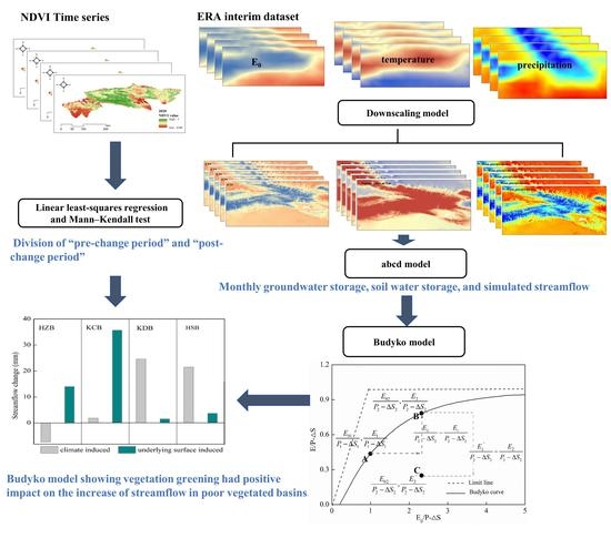
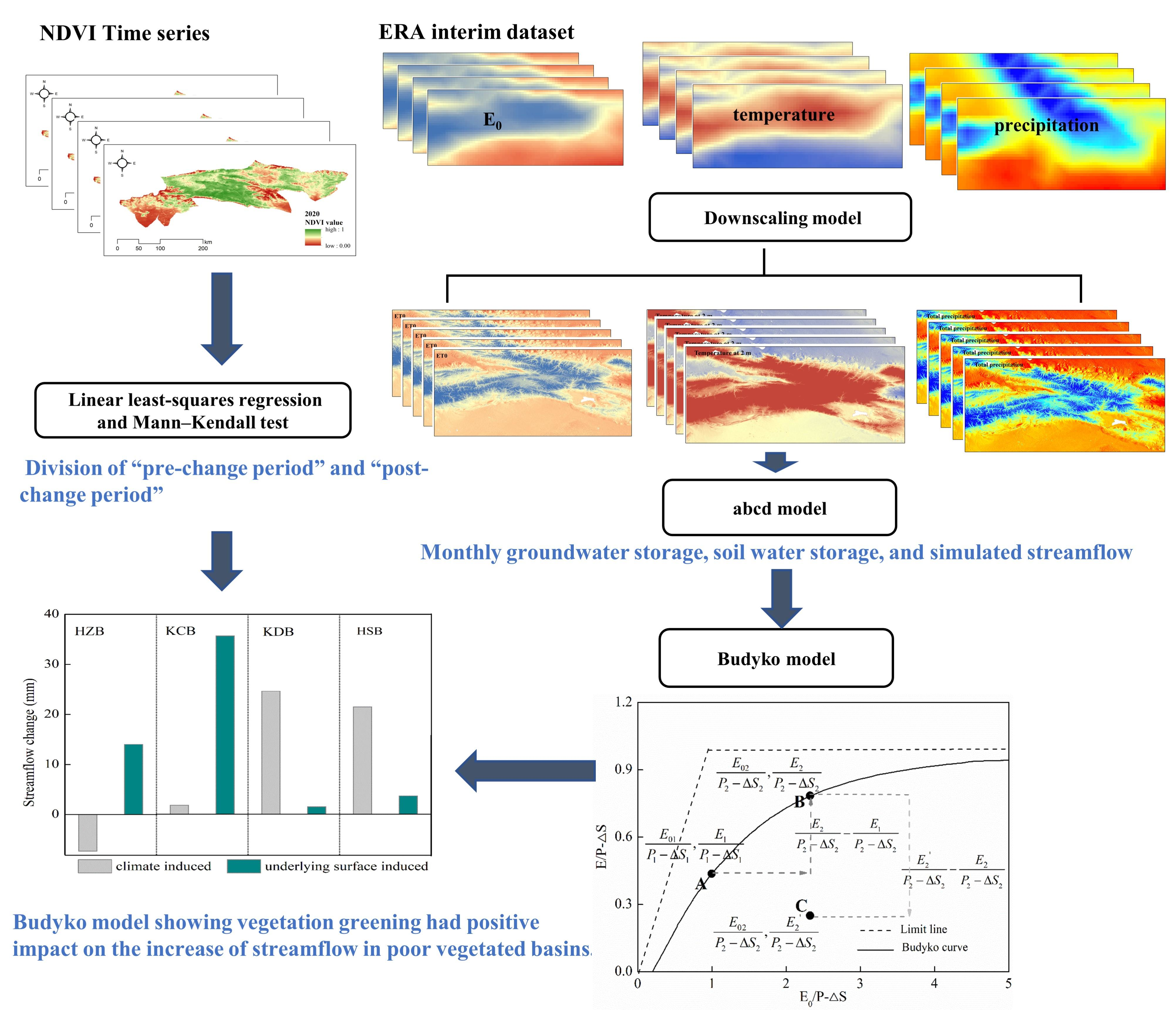
:Arid ecosystems have exhibited greening trends in recent decades. There is no consensus on how underlying surface changes influence streamflow across vegetation gradients. We investigated this issue for the four typical arid mountain basins using a 30-year runoff database and the Budyko framework to quantify the contributions of climate and underlying surface changes to streamflow variations during summer periods. Results showed that in the poor vegetated basins, i.e., Heizi Basin and Kuche Basin, the underlying surface change has increased summer streamflow by 14.01 and 35.67 mm, respectively; climate contributed only −7.32 and 1.86 mm to summer streamflow changes, respectively. Comparatively, in the well-vegetated basins, i.e., Huangshui Basin and Kaidu Basin, climate change dominated summer streamflow variations by increasing 21.50 and 24.65 mm, respectively; the underlying surface change only increased summer streamflow by 3.72 and 1.56 mm, respectively. Additionally, the decomposition results were extended to monthly scale (from June to September) to reveal the effects of climate and underlying surface changes on monthly streamflow. This study deepens our knowledge of runoff responses, which can provide important references to support water resources management in other regions that receive water from mountains.
1. Introduction
The arid region is characterized by permanent or seasonal water deficiency, which covers 41% of the earth’s surface [1]. Hydrological issues continue to dominate sustainable development in the arid region [2]. Freshwater supply in arid ecosystems plays an important role in providing staple food, cotton, and livestock to support ~38% of the global population, among whom ~50% live below the United Nations poverty line [3]. However, under the background of climate warming, the variability in water availability has been increasing, especially in arid regions. According to streamflow records from 1948 to 2016, 80% of the major rivers flowing through drylands experienced an overall decreasing trend in streamflow at the rate of −0.19 ± 0.12 mm/year [1,2]. The combination of ecological fragility and uncertainties in water availability has severely threatened sustainable development in the arid region, making it crucial to investigate the runoff responses.
Runoff dynamics are complex and closely related to precipitation, evapotranspiration, and underlying surface properties. Runoff alteration attribution analyses have been carried out with three kinds of models: (1) statistical methods such as neural network and regression models [4,5]; (2) the paired catchment method [6]; and (3) hydrological models [7,8]. Hydrological models facilitate rigorous physical interpretations and play an important role in exploring the water cycle [8]. Researchers developed hydrological models evaluating specific factors (climate or underlying surface) on streamflow by adjusting the parameter of one factor while fixing other factors, e.g., the Variable Infiltration Capacity model [9], the Soil Water Assessment Tool [8], and Budyko [7]. The Budyko framework is a decomposition method based on a conceptual hydrologic model. It has been proved to be effective in evaluating the relative influences of vegetation dynamics on the streamflow changes [7,10,11]. According to previous studies, basin streamflow can be affected by the underlying surface of basins: (1) topography and soil characteristics; (2) human activity interference; (3) and vegetation dynamics [11,12,13]. For arid basins far away from human activities and with topography, and soil characteristics being generally stable for decades, vegetation is highly controlled by water availability and is the most changeable factor [11,14]. Many researchers have been trying to find out the hydrological effects of vegetation with the Budyko model. Zhang et al. (2016) compared relations between a Budyko model parameter and vegetation across basins in China, and found that hydrological processes are more responsive to vegetation dynamics in arid regions [10,11]. Wang et al. (2012) applied the Budyko in Qinghai–Tibet Plateau and reported that vegetation degradation had negative effects on runoff variations [15]. However, researchers usually assumed that the regional water storage is balanced within many years when applying the Budyko equation [11,12,13,16], making this method limited to analysis streamflow changes at an annual scale. So far, few attempts were devoted to streamflow at a shorter time scale, such as seasonal or monthly scale. Such studies are essential due to the huge intra-annual variations of hydro-climatic variables and vegetation activities.
The Tianshan Mountains, known as the “water tower of central Asia”, provide more than 80% of the freshwater for the adjacent arid lowlands [17,18]. Streamflow in Tianshan Mountain basins were observed to increase during the streamflow peak periods (spring and summer) [17,19]. Most experts deduced that the streamflow increases were caused by increased precipitation [20] and melting water [19,21]. Hydrological effects of vegetation dynamics in the Tianshan Mountains remain unclear yet. Previous studies proposed that the enhancement of plant activity can redistribute the water fluxes between hydrosphere and atmosphere by moving blue water (streamflow) into green water (evapotranspiration) [22]. For example, in the monsoon region of China, surface runoff has experienced significant reduction after the implementation of the “Chinese forest conservation and tree planting project” since 2000 [23,24]. A recent study in the Alps also suggested that during warm summers, evapotranspiration was extremely high despite the lack of rainfall, magnifying the runoff deficit by 32% in mountain basins, eventually posing an additional threat to local water safety [22]. In contrast, some studies found that vegetation recovery can increase runoff generation by modifying inherent soil properties [25,26]. In summary, hydrological effects from land surface changes can be opposite across different basin units. The complex topographic features, as well as the interactions between water, soil and vegetation shaping the water cycle in the mountain basins, hinder the quantification of the relative impacts of climate and underlying surface changes on hydrological processes, especially on a monthly scale [22,27,28]. Quantifying how streamflow in the Tianshan Mountains were impacted seasonally and spatially is a crucial and challenging scientific issue.
Vegetation monitoring is necessary before carrying out the streamflow attribution analysis. Remote sensing technology is particularly important for vegetation monitoring in drylands, where the environment is characterized by sparse population and limited ground observations. The Normalized Difference Vegetation Index (NDVI) is one of the most widely used vegetation indices because of its high correlation with green biomass and its potential for comparing different regions through time, as the normalization minimizes effects from sun-sensor geometry, shadows, and topographic variation [29]. However, in steep mountain areas such as the Himalayas, topographic illumination and solar angle issues tend to significantly influence NDVI [30,31], leading to further development of vegetation indices, such as the Soil Adjusted Vegetation Index (SAVI) [32], Soil Adjusted Total Vegetation Index (SATVI) [33], and Enhanced Vegetation Index (EVI) [34]. According to previous studies, NDVI is still considered to be effective in reflecting vegetation growth in the Tianshan Mountains [14,35]. NDVI from satellite products, e.g., MODIS, Sentinel, Advanced Very High Resolution Radiometer sensor (AVHRR), and Landsat, consistently showed a significant positive trend in vegetation cover in most regions of the Tianshan Mountains during past decades [14,36,37], co-occurring with the enhanced evapotranspiration [38]. As for the data availability, NDVI data from MODIS were not available until 2000; and NDVI from the Landsat TM/ETM+ series were not suitable for seasonal vegetation monitoring because of the influences from the missing values and problematic pixels [29]. NDVI data from Global Inventory Modeling and Mapping Studies (GIMMS) have been widely used in vegetation monitoring [29,33]. Despite its relatively coarse spatial resolution (~8 km), GIMMS has the longest time series, spanning from 1981 to 2015 and a half-month temporal resolution, which greatly enhanced the utility of remote sensing for large-scale analysis of seasonal cycles of vegetation activity [29,36]. In this study, we applied GIMMS NDVI to evaluate the restoration/degradation condition of vegetation in the Tianshan Mountains.
In addition, the current streamflow simulations were almost based on observation data from meteorological stations. The simulation accuracy is strongly dependent on the density and distribution of the meteorological stations. However, the Tianshan Mountains, with only 23 stations distributed, covering more than 500,000 km2, create great challenges for accurate streamflow simulations. Therefore, earth system data products along with downscaling techniques are urgently needed for application of the Budyko model in ungauged basins.
There are two issues that urgently need to be addressed: (1) how to increase simulation accuracy with the limited meteorological stations and (2) to what extent the mountain basin streamflow can be affected by underlying surface change vs. climate change at seasonally/monthly scale. Here, to overcome these issues, we reconstructed the high-resolution precipitation, temperature, and potential evapotranspiration based on ground observations and the earth system data products. The GIMMS NDVI was applied to estimate vegetation restoration/degradation during study periods, and the Budyko decomposition method was extended to the seasonally/monthly scale by integrating a monthly abcd model, which can calculate regional water storage variations. The study aims to quantify the contributions of climate and underlying surface changes to seasonally/monthly streamflow changes in the arid Tianshan Mountain basins. The results are of great theoretical and practical significance for estimating hydrological effects from underlying surface changes in arid mountain basins.
2. Materials and Methods
2.1. Study Area
The Tianshan Mountains, located in the Eurasia hinterland, are far from the sea and ocean. They consist of a series of mountains, basins, and valleys. The Tianshan Mountains release a great quantity water sources to most of the local rivers and lakes through a combination of meltwater in the high-mountain area, precipitation in the mid-mountain area, and fissure water in the low-mountain area, especially during summer [18]. Because the inland location is associated with a continental climate and scarce precipitation, streamflow from mountain basins are the most important water resources for the downstream oasis agriculture, production, and living activities [19].
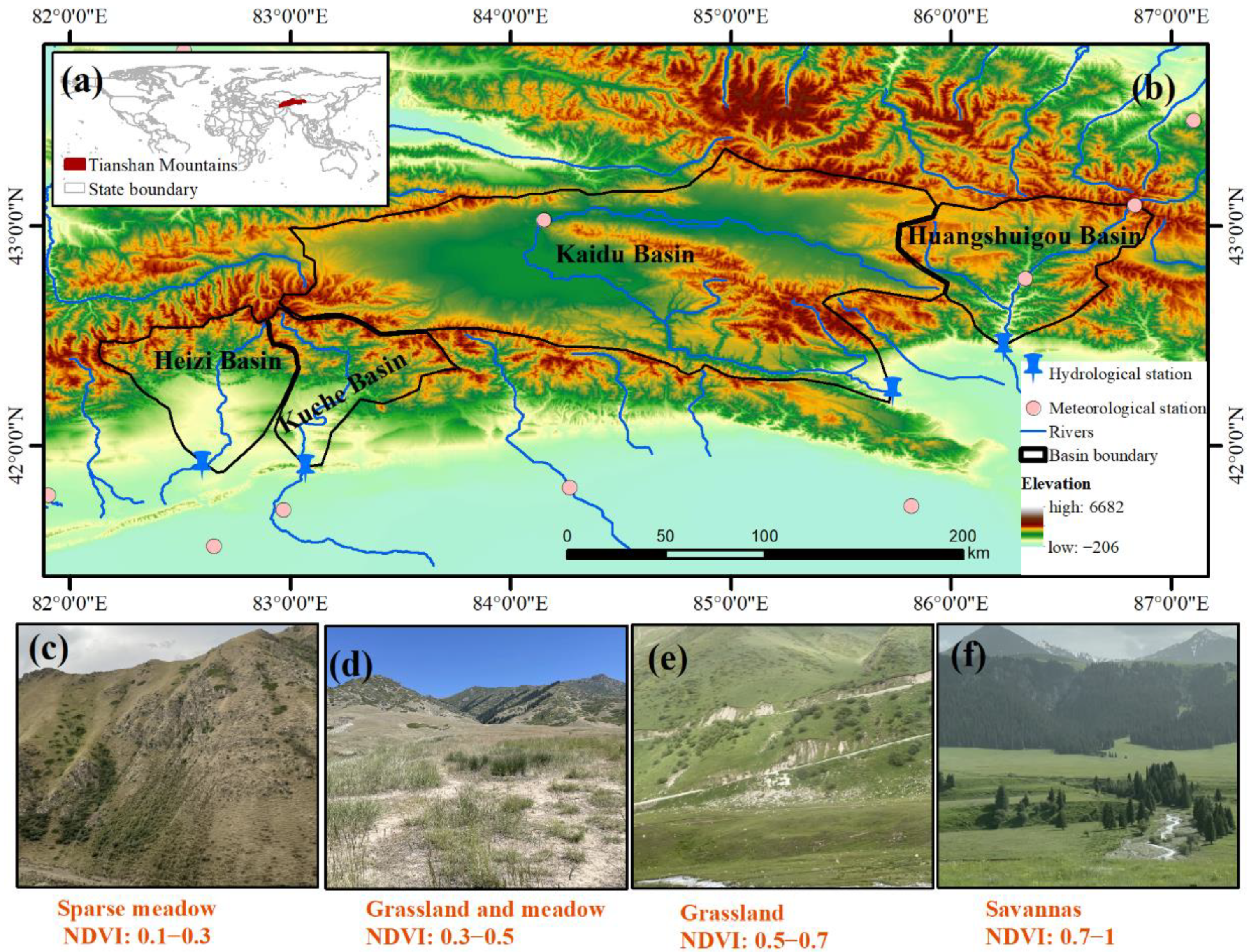
This study selected four basins in the southern Tianshan Mountains: Heizi Basin (HZB); Kuche Basin (KCB); Kaidu Basin (KDB); and Huangshui Basin (HSB) (Figure 1). HZB (41.87−42.64°N, 82.14−83.04°E) covers an area of 3342 km2, and the elevation ranges from 1320 to 4760 m; KCB (41.87−42.60°N, 82.92−83.80°E) covers an area of 2946 km2, with an elevation range from 1380 to 4480 m; KDB (42.17−43.34°N, 82.83−85.98°E) covers an area of 18,827 km2, with an elevation range from 1340 to 4742 m; and HSB (42.45−43.13°N, 85.76−86.90°E) covers an area of 4311 km2, with an elevation range from 1327 to 4324 m. The four basins are adjacent to each other and are far from human activities. Because of the scarce annual precipitation, which ranges from 200 to 600 mm, the vegetation growth pattern is highly dependent on water availability. Specifically, in HZB and KCB, vegetation type is dominated by sparse meadow and grassland. In HSB, grass and meadow cover more densely with some low shrubs by the river. In the valley of KDB, where terrain is flat and precipitation is abundant, vegetation is characterized by savannas (Figure A1). Generally, ranking of the regional mean greenness of the four basins is as follows: KDB (NDVI = 0.65) > HSB (NDVI = 0.50) > KCB (NDVI = 0.38) > HZB (NDVI = 0.31) (Figure A2). In summary, the four basins are representative in terms of landscapes and vegetation greenness.
2.2. Data Sources
Vegetation conditions of the four basins from 1983 to 2012 were evaluated using the GIMMS NDVI product (https://ecocast.arc.nasa.gov/data/pub/gimms/, accessed on 1 May 2021) [33]. All available images were selected to evaluate vegetation restoration/degradation. To estimate peak pasture productivity within the four basins, we extracted the summer maximum NDVI for each grid cell and for each study year, as detected by GIMMS.
Streamflow of the four mountain basins was recorded by their respective mountain exit stations. Monthly average streamflow of HZB (1980−2006), KCB (1980−2006), KDB (1980−2012), and HSB (1980−2008) was collected from Xinjiang Hydrology Bureau.
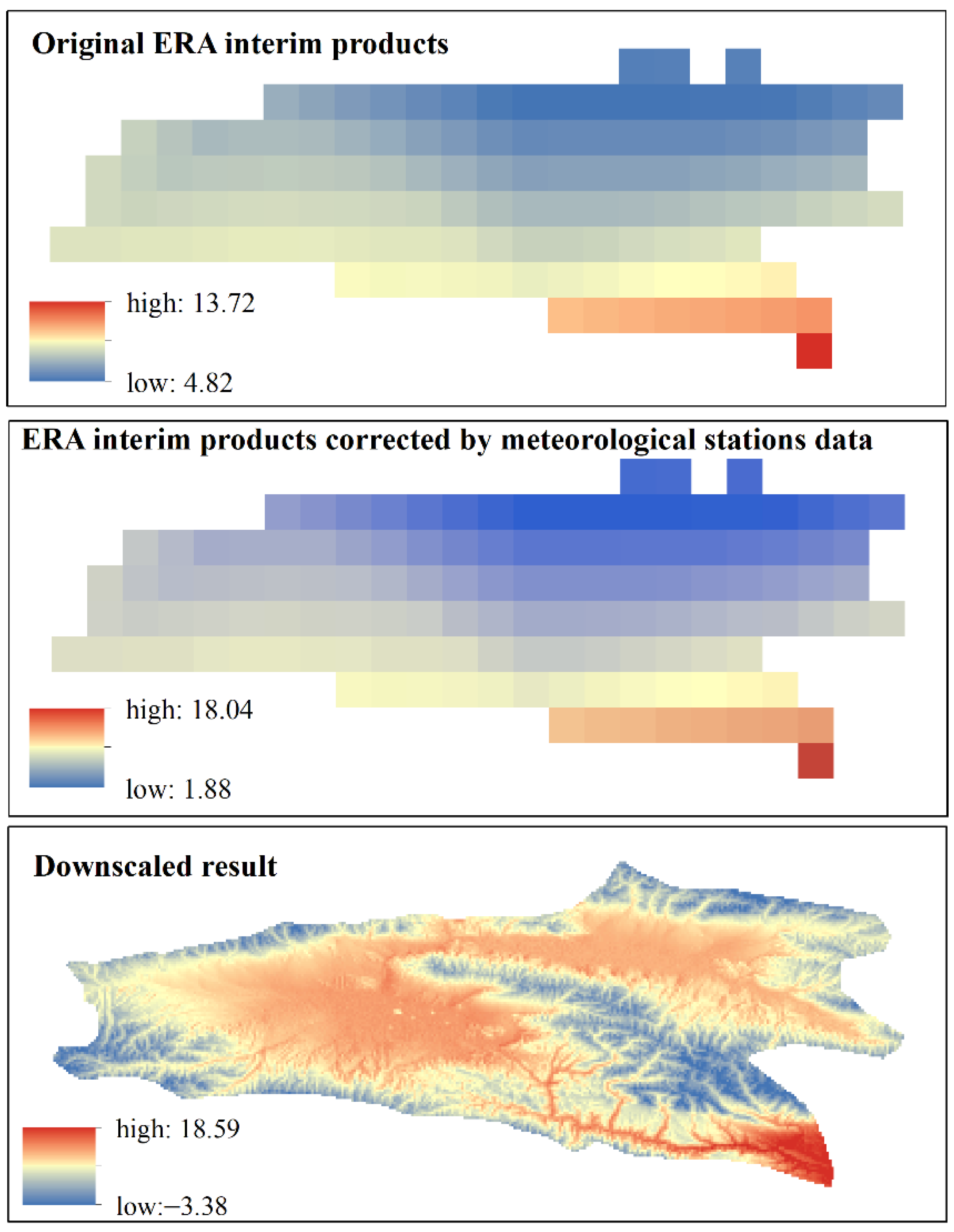
Meteorological stations in and around the four basins are extremely limited, bringing about challenges for accurate streamflow simulation. In this study, we collected ERA interim daily averaged data from 1980 to 2012 (https://apps.ecmwf.int/datasets/data/interim-full-daily, accessed on 1 May 2021). The ERA interim is a daily dataset with a spatial resolution of 0.125°. Climate data includes total precipitation, maximum/minimum/mean temperature at 2 m, wind speed, surface pressure, and sunshine duration. To obtain the more accurate basin climate dataset, we applied the downscaling model to reconstruct the climate condition of the four basins from 1980 to 2012. Reconstruction of the climate dataset consisted of the following steps: (1) preliminary correction of ERA interim products using original meteorological station data; (2) extracting terrain variables, i.e., elevation, slope, aspect, and topographic wetness index with the resolution of 1 km from SRTM-DEM product (https://srtm.csi.cgiar.org/, accessed on 1 May 2021); (3) resampling the terrain variables to 0.125° resolution; (4) obtaining fitting formula between resampled terrain variables and ERA interim climate variables using multiple methods, e.g., linear regression, random forest, and support vector machine; (5) using the high resolution (1 km) terrain variables to reconstruct the high resolution (1 km) climate dataset by applying the optimal fitting formula (Figure A3); (6) verification using the meteorological station data [39,40,41].
2.3. Trend Analysis
Change trends in vegetation greenness and streamflow were determined using the slope of the linear least-squares regression [42] and Mann–Kendall (MK) test [43]. The MK test, as a non-parametric test widely used to investigate trends in time series, was applied to examine the significance of change trends in annual/seasonal streamflow and summer maximum NDVI for the four basins. The null hypothesis, that there is “no trend” at the 0.95 confidence level, was applied when using the MK test. There is a rising trend if the slope of change (z) > 0, and vice versa there is a decreasing trend [43]. In addition, Pettitt’s test was applied to detect the probable single change point of variables within a certain year during the study period [44].
2.4. Monthly Water Storage Change Calculation Based on Abcd Model
To calculate monthly available precipitation, the abcd model was applied to simulate streamflow and to calculate water storage (S, sum of ground water storage and soil water storage). The traditional abcd model takes monthly precipitation and potential evapotranspiration as input variables, and generates monthly groundwater storage, soil water storage, and simulated streamflow as output [45]. As the name says, this model includes four parameters, i.e., a, b, c, and d. Parameter a ranges from 0 to 1 and is the probability of the runoff occurring without the soil being fully saturated; parameter b is the maximum limit of soil water storage and evapotranspiration; parameter c (0~1) is the proportion of streamflow from groundwater; parameter d (0~1) is the relation coefficient for groundwater discharge and storage [45]. The above four parameters needed to be calibrated during simulation.
In the four mountain basins, the form of precipitation is snow for quite a long time. The form of precipitation (snow or rain) is influential for the streamflow formation and transformation. Therefore, the snow fall, snow/ice storage, and melting processes were taken into account by applying the degree-day model. If daily temperature is lower than 0 °C, both snow and rain fall will be temporarily stored as snow/ice instead of forming runoff, while if daily temperature is higher than 0 °C, stored ice/snow will melt to generate runoff. The amount of melting water is evaluated empirically according to daily air temperature and then added to precipitation instead of being directly discharged into rivers/lakes [46]. Snowmelt-related parameters (a1 and a2) were added into the abcd model in this study.
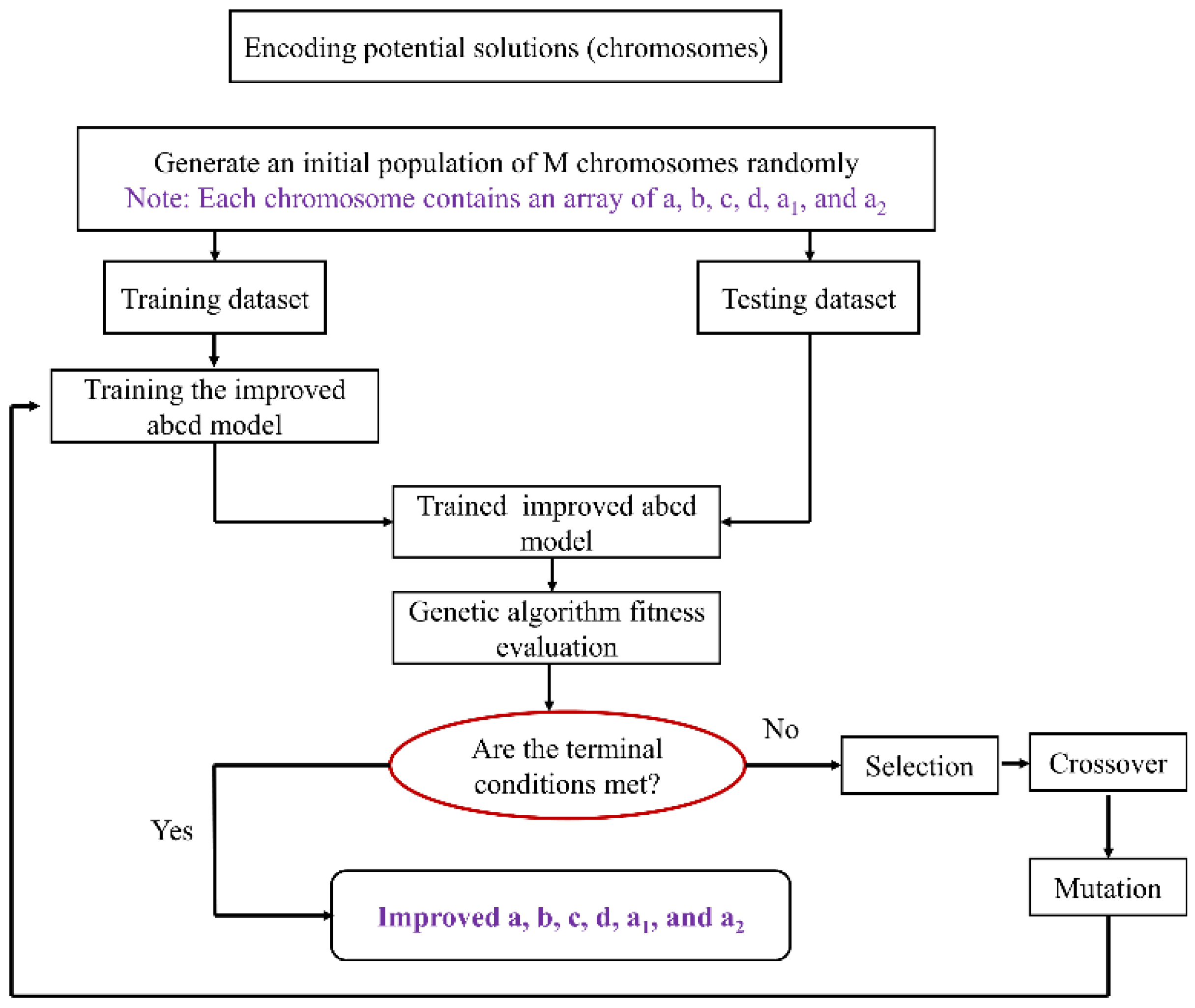
Parameters a, b, c, d, and snowmelt-related parameters (a1 and a2) were determined by using a genetic algorithm. Genetic algorithm is a method for solving engineering optimization problems that is based on natural selection, which repeatedly modifies a population of individual solutions. At each step, the genetic algorithm selects individuals randomly from the current population to be parents and uses them to produce the children for the next generation. Over successive generations, the population “evolves” toward an optimal solution [47,48]. Parameters optimization with genetic algorithm was completed in MATLAB. The flowchart of the parameter optimization base on genetic algorithm has been supplemented in Figure A4.
The initial groundwater storage, soil water storage, and snow depth were determined during the preheating period (e.g., 1980−1982 in this study). Nash–Sutcliffe efficiency coefficient (NSE) was applied to evaluate the model performance, which can be expressed as follows:
where and represent the observed and simulated values, respectively.
2.5. Budyko Decomposition Method Extended by Abcd Model
The Budyko model provides an effective way for calculating the relative impacts of climate and underlying surface changes on streamflow accurately [49,50]. But there is a presupposition for the traditional Budyko model that water storage is balanced for the long term, which hinders the identification of seasonal streamflow change causes [49]. To incorporate the seasonal effects on water balance, we added the water storage variable (S), which is derived from the abcd model, to obtain the monthly available precipitation [15,50]. The extended Budyko model is as follows:
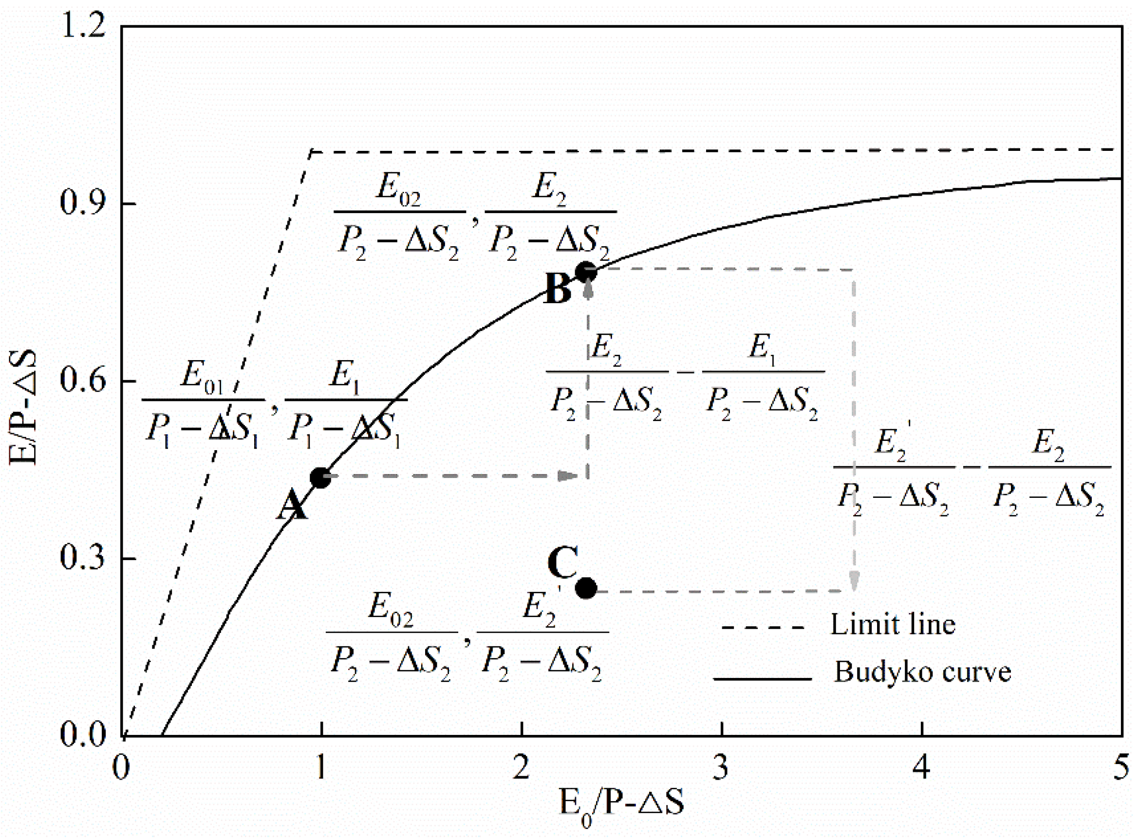
where , and are the mean annual actual evapotranspiration, mean annual potential evaporation, and mean annual precipitation, respectively; is seasonal water storage change. The monthly is calculated using the Penman–Monteith equation [51]; the monthly and are calculated based on monthly and using the abcd model. is an empirical parameter subjected to be calibrated, and controls the shape of the Budyko curve [50].
The Budyko curve is shown in Figure 2. The Budyko model assumes that for a basin without underlying surface change and human interference, if climate condition becomes wetter or drier, the evaporation ratio will also adjust its position along the Budyko curve, e.g., from point A (pre-change period) to point B (post change period) in Figure 2, whereas with the underlying and human activities affect, point B will be changed to point C. Therefore, for the four basins without human interference, the underlying surface change induced streamflow changes can be calculated as follows:
where is the streamflow changes induced by underlying surface changes. The streamflow change induced by climate () is calculated by subtracting from the total streamflow change :
where is the difference in streamflow between the pre-change period () and post-change period ():
In summary, the extended Budyko model is carried out as follows: (1) using the daily total precipitation, maximum/minimum/mean temperature at 2 m, wind speed, surface pressure, and sunshine duration and the Penman–Monteith equation to calculate daily , and adding the daily value to get the monthly ; (2) using the daily , and temperature dataset and the abcd model to simulate monthly streamflow in the four basins, and obtain the monthly and ; (3) the parameters are calibrated at both seasonal and monthly time scale according to Equation (2); (4) compute the climate and underlying induced changes in streamflow based on Equation (3) and (4).
3. Results
3.1. Change Trends in Basin Vegetation
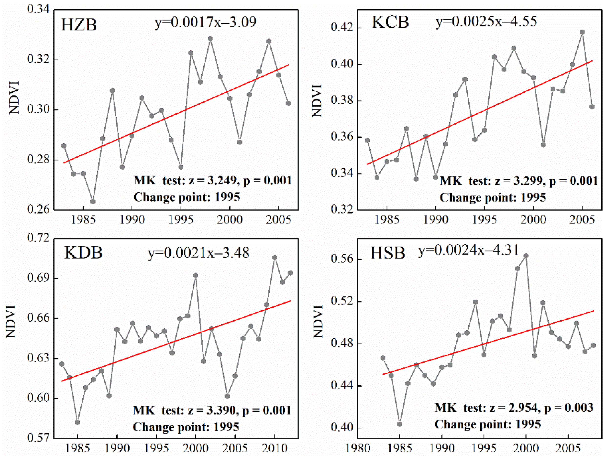
A multiyear phenological curve shows that vegetation of the four basins completes the “green up” processes in June and starts to wither after September (Figure 3). Therefore, June to September (summer) from 1983 to 2012 were selected as the study period. In addition, annual trends of summer maximum NDVI in HZB, KCB, KDB, and HSB increased significantly (p < 0.05), with the z value of 3.249, 3.299, 3.390, and 2.954, respectively. The change point indicates the year during which the vegetation greenness experienced an inflection; it can be calculated by Pettitt’s test. In all of the four basins, summer maximum NDVI values inflected in 1995 (Figure 4). In summary, vegetation in the four basins experienced overall greening trends during past decades; the single change points of vegetation greenness occurred in 1995. Therefore, the years from 1983 to 1995 were defined as “pre-change period” and those after 1995 were defined as “post-change period”.
3.2. Streamflow Variations of the Four Basins
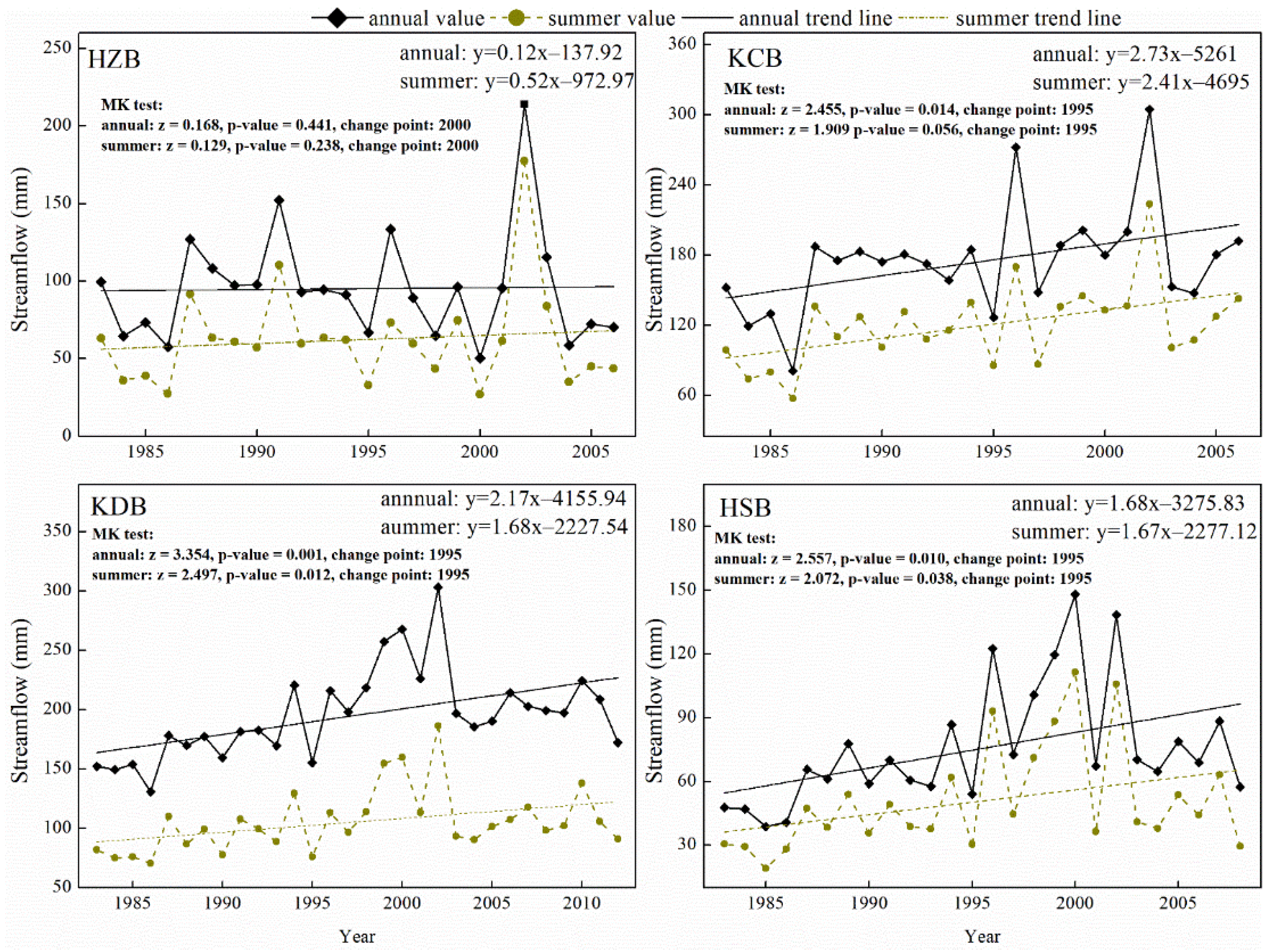
Both annual and summer streamflow of the four basins all showed upward trends during the study periods (Figure 5). In HZB, summer streamflow accounts for about two-thirds of the annual streamflow. Both annual and summer streamflow changed slightly with the increase rates of 0.12 and 0.52 mm/year, respectively, and reached their highest values of 214.04 mm and 117.39 mm, respectively, in 2002. In KCB, annual and summer streamflow increased significantly with the rates of 2.73 and 2.41 mm/year, and peaked with the values of 304.69 and 223.67 mm, respectively, in 2002. In KDB, summer streamflow accounts for about half of the annual streamflow. Annual and summer streamflow increased at the rates of 2.17 and 1.68 mm/year, respectively, and peaked in 2002 with the values of 303.23 and 186.29 mm, respectively. In HSB, summer streamflow accounts for more than three-fourths of the annual streamflow. Annual and summer streamflow shared very similar change trends and they increased at the rates of 1.68 and 1.67 mm/year, respectively. Annual and summer streamflow peaked in 2000 with the values of 148.17 and 111.58 mm, respectively.
In addition, the significance of streamflow change trends was checked by using the MK test. In HZB, both annual and summer streamflow trends were not significant (p > 0.05). In KCB, KDB, and HSB, annual streamflow changed significantly (p < 0.05) with the z values of 2.73, 2.17, and 1.68, respectively. Summer streamflow in these three basins showed similar significant trends with the z values of 2.41, 1.68, and 1.67, respectively. The change point as detected by Pettitt’s test showed the year during which the streamflow experienced an inflection. In HZB, both annual and summer stream flow inflected in 2000, while in KCB, KDB, and HSB, both annual and summer stream flow inflected in 1995.
3.3. Fitting Results of Abcd Model
The abcd model was applied to calculate water storage change and the actual evaporation for further identification of causes of seasonal streamflow changes. The extended abcd model takes , , and temperature as input, and generates monthly soil moisture, groundwater, and simulated streamflow as output. A preheating period is necessary for getting the initial ground water storage, soil water storage, and snow depth. We tested many times and found the abcd model became robust during the third year. Therefore, the period 1980−1982 was set as the preheating period in this study. Considering that vegetation experienced greening after 1995, the study period was divided into pre-change (1983−1995) and post-change periods (after 1995), and either period was subdivided into calibration period and validation period. Model parameters were calibrated separately during the pre-change and post-change period using the genetic algorithm, and were summarized in Table A1.
Figure 6 shows the observed and simulated streamflow of the four basins. The abcd model performance was evaluated by the NSE (Table 1). NSE values of the four basins were all above 0.7 during both calibration period and validation period, meeting the requirements for further analysis. Monthly water storage change () was then obtained (Figure A5) for calculating monthly available water ().
3.4. Quantification of Climate and Underlying Impacts on Summer Streamflow
Given that vegetation greenness peaks in summer and summer streamflow accounts for more than half of the annual streamflow, here we only focus on the causes of summer (June to September) streamflow changes. Monthly available water () and derived from abcd model, and were taken as an input variable into the extended Budyko model to calibrate , and further to calculate the relative impacts of climate change and underlying surface change on seasonal and monthly streamflow changes. The values of climatic and hydrological variables of the four basins during summer are shown in Table 2.
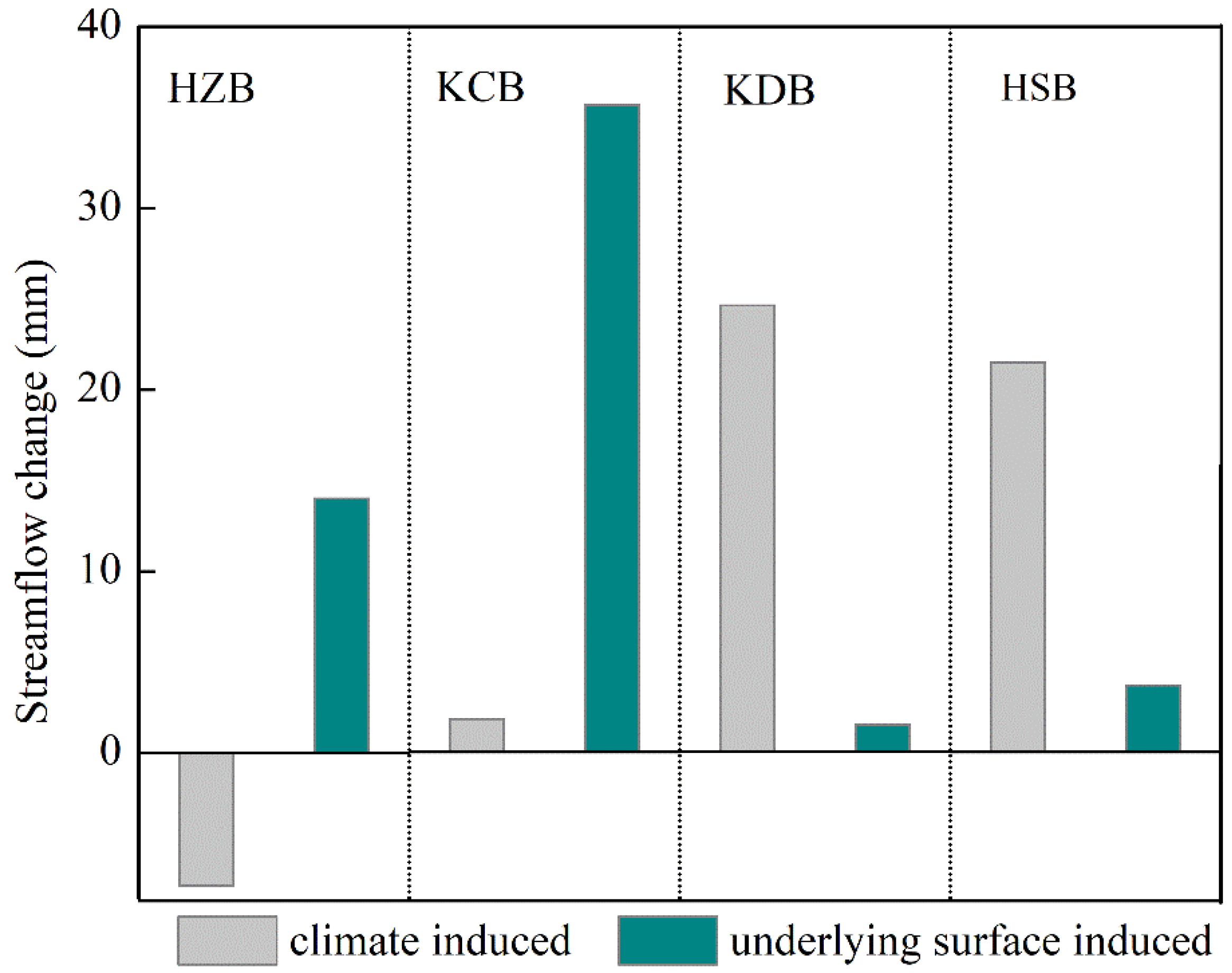
The relative impacts of climate and underlying surface change on annual and seasonal streamflow changes were quantified using the Budyko model. Figure 7 presents the quantification results of the climate-induced and underlying surface-induced changes in streamflow during summer. Climate change has increased streamflow in KDB, HSB, and KCB with the values of 24.65, 21.50, and 1.86 mm, respectively, and has decreased streamflow in HZB with the value of −7.32 mm. Underlying surface change has increased streamflow in all four basins, with the contribution degree ranked as follows: KCB (35.67 mm) > HZB (14.01 mm) > HSB (3.72 mm) > KDB (1.56 mm). It is worth noting that in watersheds with poor vegetation conditions (i.e., KCB and HZB), vegetation recovery exerted a greater influence on streamflow, while in those watersheds with flourishing vegetation (KDB and HSB), climate is more influential for streamflow.
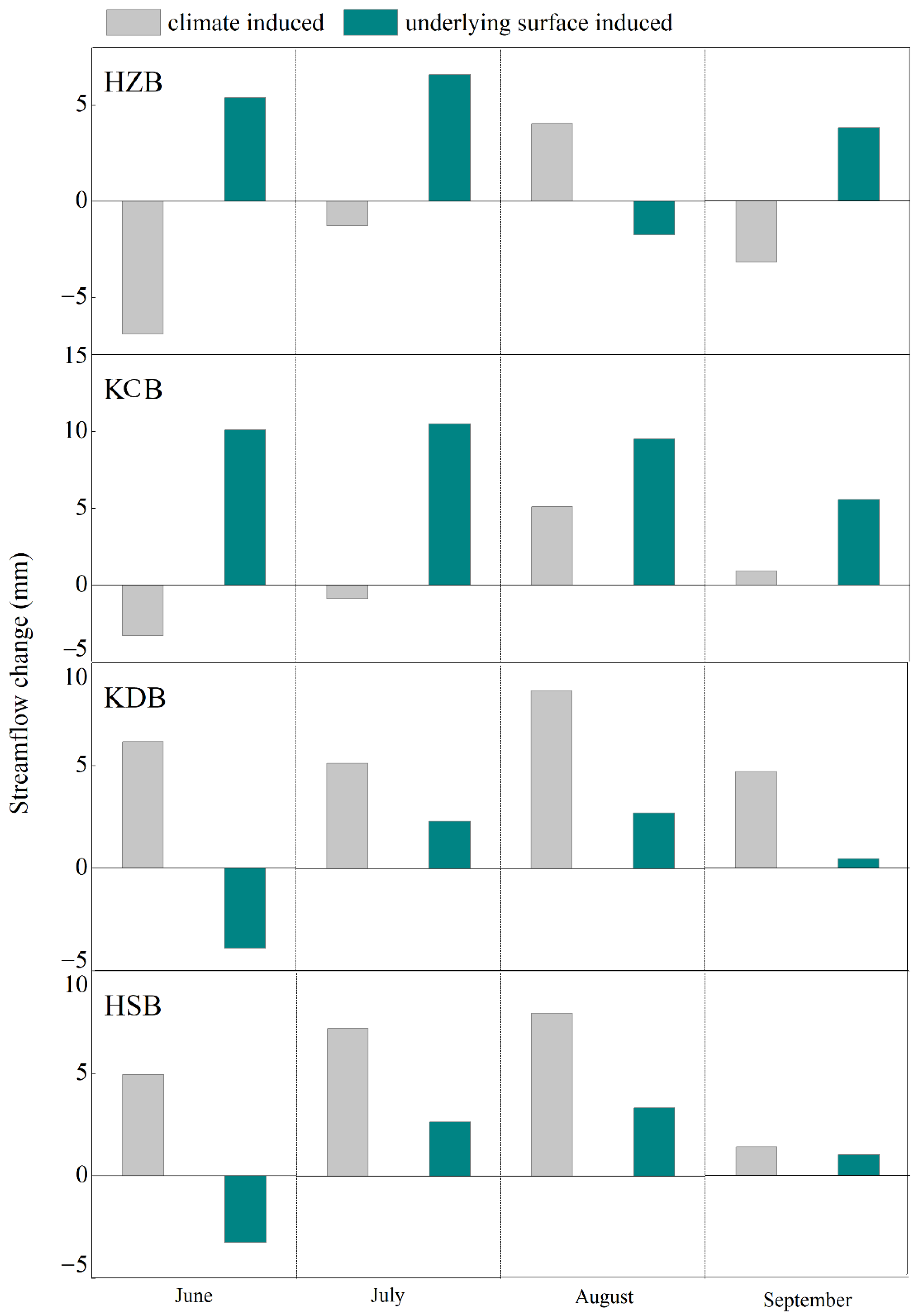
Figure 8 presents the quantification results of the climate-induced and underlying surface-induced changes in streamflow for each summer month. In HZB, the underlying surface change can increase streamflow in June, July, and September, with the values of 5.38, 6.58, and 3.82 mm, but decrease streamflow in August with the value of −1.77 mm. By contrast, climate decreases streamflow in June, July, and September, with the values of −6.92, −1.28, and −3.17 mm, but increases streamflow in August with the value of 4.04 mm. In KCB, underlying surface changes exerted strong influences on streamflow and increased streamflow in all four months, with the increase values of 10.09, 10.50, 9.51, and 5.57 mm, respectively; climate change exerted smaller influences on streamflow as compared with underlying surface change. Climate change decreased streamflow in KCB in June and July, with the values of −3.28 and −0.88 mm, respectively, and increased streamflow in August and September with the values of 5.09 and 0.93 mm, respectively. Streamflow in KDB was dominated by climate change in all four months. Specifically, climate change increased streamflow in KDB in June, July, August, and September, with the values of 6.17, 5.11, 8.65, and 4.72 mm, respectively; the underlying surface change decreased streamflow in June (−3.90 mm), and increased streamflow in July (2.28 mm), August (2.70 mm), and September (0.47 mm). In HSB, streamflow was also dominated by climate change. During June, July, August, and September, climate change increased streamflow, with the values of 4.95, 7.19, 7.94, and 1.42 mm, respectively; underlying surface change decreased streamflow in June (−3.25 mm) and increased streamflow in July, August, and September, with the values of 2.63, 3.32, and 1.03 mm, respectively. The monthly results are consistent with the seasonal results, suggesting that streamflow in the poor vegetated basins is more susceptible to underlying surface change while the streamflow in well-vegetated basins is dominated by climate change.
4. Discussion
4.1. Vegetation and Hydrological Changes in Arid Mountain Basins
We detected some major changes in the arid Tianshan Mountain basins. First, mountain basins have generally become greener. Second, basin streamflow increased in recent decades.
Arid ecosystems are among the most vulnerable to climate change. Previous studies have revealed atmospheric drying from multiple meteorological indexes (e.g., vapor pressure deficit and aridity index) [1]. Counterintuitively, the world’s arid regions have exhibited significant greening and enhanced vegetation productivity in recent decades [52]. In this study, the summer maximum value of NDVI from GIMMS observations also consistently showed a significant positive trend in vegetation cover of arid mountain basins from 1983 to 2012. The greening trends under the climate warming and atmospheric drying were found to be related to the warming and wetting trends in Northwest China [37], as well as the plant physiological regulations of evapotranspiration under elevated CO2 according to Lian et al. [1]. We also found that the summer maximum NDVI values were much higher after 1995, suggesting the recovery of vegetation in the four mountain basins during post-change periods (from 1996 to 2012).
Despite that the streamflow of the major rivers in drylands showed decrease trends, streamflow from the four arid mountains basins in Tianshan have exhibited upward trends, co-occurring with the expansion of other surface water storages (e.g., lake expansion) [53]. However, the streamflow increase in mountain basins has not eliminated water pressure on agriculture in lower plain lands, as the irrigation area and the population continued to increase. For example, in Xinjiang (China), the largest administrative region directly receives water from the four mountain basins and is highly dependent on agriculture, which consumes more than 90% of local available freshwater [17]. Since the 1990s, the total farming lands in Xinjiang have increased by 47.87%, with water-intensive crops (e.g., cotton and vegetables) increasing most rapidly. In addition, per capita available water in Xinjiang has decreased by 32.23%. Therefore, despite that the streamflow from mountain basins is increasing, water shortage in arid lowlands around the Tianshan Mountains will still be the major threat to regional development.
4.2. Impact of Underlying Surface Change on Streamflow
A sudden increase in woody plants can significantly increase root water absorption, leaf interception, and actual evapotranspiration, which can lead to the surge of ecological water, resulting in the reduction of runoff [17,24]. Comparatively, in the Tianshan Mountain basins, vegetation experienced a slight recovery without human interference. Such slight recovery increased streamflow instead, and the contribution of underlying surface change even surpassed climate change, especially in those basins with poor vegetation condition. There are several reasons why the vegetation recovery in the Tianshan Mountains could increase streamflow. First, the Tianshan Mountains are characterized by the arid continental climate and long distance from ocean water vapor. Most basins are not well vegetated under insufficient precipitation, especially in HZB and KCB where the vegetation is dominated by sparse meadow and summer NDVI is about 0.3. The soil is sandy and rocky, and is underdeveloped [28]. Therefore, the slight recovery of vegetation can help increase soil water holding capacity and leaf interception, which can help converse precipitation to surface runoff immediately. Wang et al. (2012) also found that in the Qinghai Tibet Plateau, grass and meadow degradation in watersheds with large slope can significantly reduce soil and water content, and eventually reduce both surface and subsurface runoff [15]. Secondly, ecological water demand of grass and meadow is much smaller as compared with forest, especially in those basins with a barren underlying surface. Therefore, the contribution of vegetation recovery to actual evapotranspiration is negligible and could not reduce surface runoff.
We further quantified the contribution of underlying surface change to streamflow change in four basins with different vegetation conditions, i.e., KDB (NDVI = 0.65), HSB (NDVI = 0.50), KCB (NDVI = 0.38), and HZB (NDVI = 0.31). They all experienced slight vegetation greening from 1981 to 2012 according to their summer max NDVI change trends (Figure 4). However, the contribution of vegetation recovery to streamflow changes varied greatly across the four basins. Underlying surface change induced the greatest streamflow increases in poorly vegetated basins (i.e., KCB and HZB), medium streamflow increases in moderately vegetated basins (HSB), and the smallest streamflow increases in the best-vegetated basins (KDB). This can be well explained by their underlying conditions. In barren basins such as KCB and HZB, soil is most underdeveloped and is characterized by loose soil particles and insufficient water-holding capacity. Precipitation in the four basins is usually small and lasts for a short period of time, and they infiltrate before confluence, making it difficult to form surface runoff. Slight vegetation recovery can greatly improve the situation of the underlying surface by improving soil development, reducing water and soil loss, and increasing leaf interception [54]. However, things are quite different in the well-vegetated KDB, where savannas are widely distributed in the river valley, which consists of a considerable part of woodland. Summer NDVI in KDB experienced similar trends as other basins, but their contribution to streamflow changes was negligible. The above can be explained by the huge ecological water consumption of forest, which is almost three times that of grassland [55]. In addition, soil in the well-vegetated KDB is better developed as compared with that in KCB and HZB, and therefore the increase of surface interception is limited. Streamflow increase induced by improved underlying surface can easily be offset by the larger ecological water consumption. In summary, streamflow in poorly vegetated basins is greatly affected by underlying surface change, while in well-vegetated basins, streamflow is dominated by climate change.
4.3. Implications
The Tianshan Mountains are the water tower of central Asia as well as the region’s ecological barrier. Vegetation recovery and increased mountain streamflow seem to indicate a better ecological environment in central Asia. However, in the meantime, natural vegetation in some plain areas is deteriorating due to the risk of water shortage. For example, in the oasis-desert ecotone of the southern Tianshan Mountains, vegetation communities sensitive to precipitation (e.g., Agriophyllum squarrosum and Artemisia arenaria) are disappearing, while those insensitive to water availability (e.g., Calligonum mongolicum and Nitraria tangutorum) are gradually expanding [56], leading to a reduction in biodiversity and ecological imbalance [56]. In addition, the river cessation in the downstream areas of the Tarim River is also worthy of attention, which occurred as a result of several processes [57], including human water consumption, dropdown of ground water level, and lake disappearance [53]. Such divergence between alpine and low plain eco-environment changes is noteworthy. Whether the vegetation recovery in alpine mountains has occupied water in low plain and finally led to ecological deterioration, is a subject in need of further research.
This study concentrated on the relative impacts of underlying surface change on mountain basin streamflow. Different from the previous findings in the forested Alps [22], in which the increase of alpine forest increased actual evapotranspiration and amplified the runoff deficit, this study showed that in the poorly vegetated Tianshan Mountains, vegetation recovery has not consumed water excessively and has benefited for streamflow increase. Overall, the runoff database and the Budyko framework used in this study offer a good representation of assessing the hydrological effects of vegetation in poorly vegetated mountain basins. However, the latest runoff datasets (after 2013) were not available for this study, leading to ignorance about the latest feedback of vegetation on runoff. The latest summer maximum NDVI from MODIS (http://e4ftl01.cr.usgs.gov/MOLT, accessed on 1 May 2022) indicated that vegetation in the Tianshan Mountains is still recovering in the recent decade and there is a trend of vegetation expansion to high altitude (Figure A6). This phenomenon may indicate an improved alpine eco-environment. But it is worth noting that the positive feedback of vegetation on streamflow change may take a new turn as global warming continues and evapotranspiration continues to increase. Long-term observation of streamflow and alpine eco-environment is underway and is the focus of our future work.
5. Conclusions
This study compared summer streamflow variations and their response to climate and underlying surface changes in four typical mountain basins. We concluded that: (1) Summer streamflow of the four basins experienced upward trends over past three decades; (2) In the poorly vegetated basins (i.e., HZB and KCB), vegetation greening had a positive impact on the increase of streamflow while climate changes had little impact; (3) In the well-vegetated basins (i.e., HSB and KDB), climate change dominated streamflow while underlying surface change had little impact. The experience of vegetation recovery in the Tianshan Mountains and its positive effects on streamflow in poorly vegetated basins exemplified ecological rehabilitation in alpine mountains of central Asia. However, as the global temperature and evapotranspiration continue to increase, relations between vegetation dynamics and hydrological cycle need long-term attention.
Author Contributions
Conceptualization, L.Z. and J.X.; formal analysis, L.Z.; funding acquisition, J.X.; investigation, L.Z.; methodology, Y.C. and Z.W.; resources, Z.W.; software, Y.C.; writing—original draft, L.Z.; writing—review and editing, J.X. All authors have read and agreed to the published version of the manuscript.
Funding
This work was supported by East China Normal University Excellent Doctoral Students’ academic innovation ability improvement plan project (YBNLTS2021-028) and the National Natural Science Foundation of China (Grant No. 41871025, U1903208, 41630859).
Data Availability Statement
All data, models or code generated or used during the study are available from the corresponding author by request.
Conflicts of Interest
We declare that we have no financial and personal relationships with other people or organizations that can inappropriately influence our work, there is no professional or other personal interest of any nature or kind in any product, service and/or company that could be construed as influencing the position presented in the manuscript entitled “Increasing streamflow in poor vegetated mountain basins induced by greening of underlying surface”.
Appendix A
Figure A1.
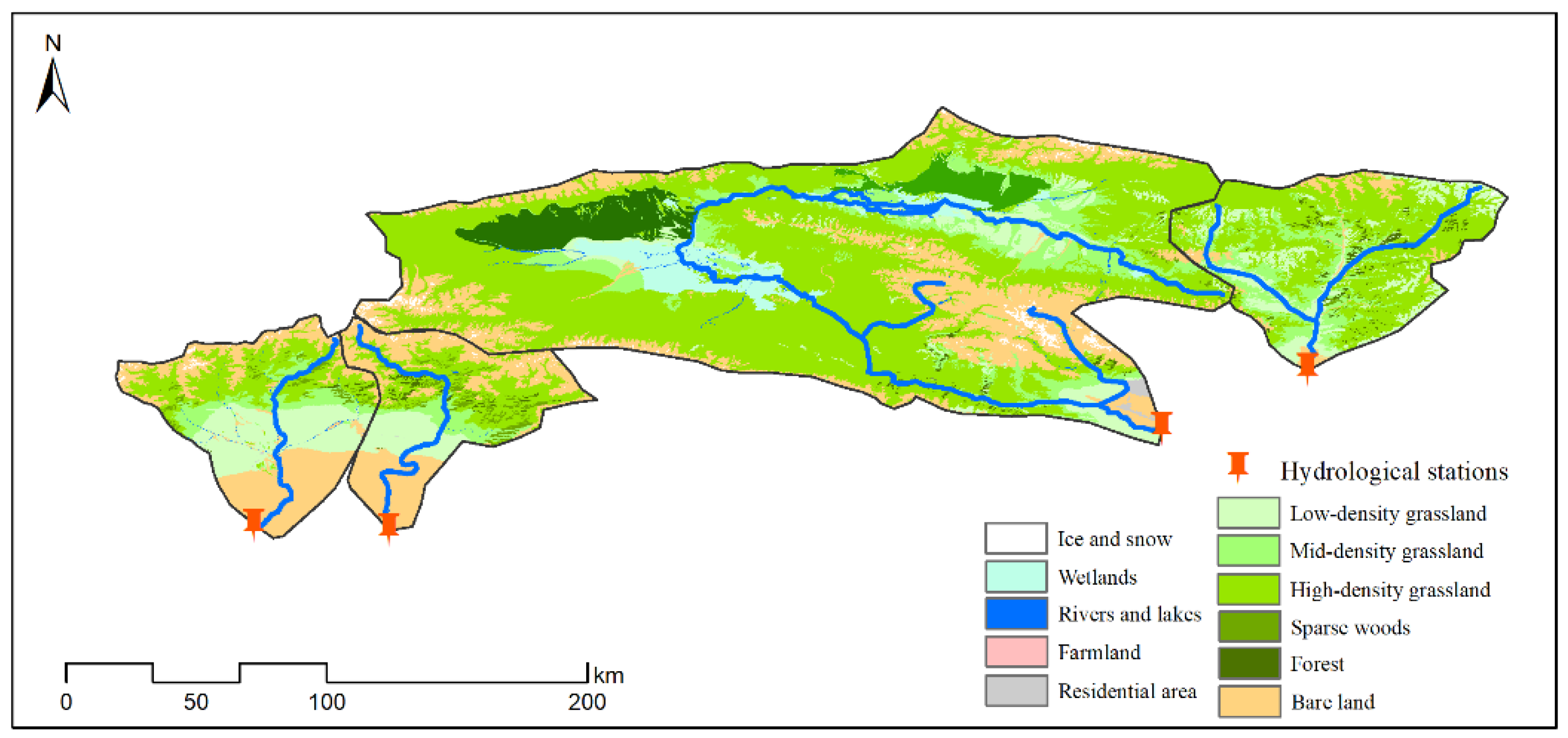
Land cover classification map for the four basins. This map has a spatial resolution of 30 m and was derived from Landsat images during 2010. The dataset is by provided by Data Center for Resources and Environmental Sciences, Chinese Academy of Sciences (RESDC) (http://www.resdc.cn, accessed on 1 May 2021).
Figure A1.
Land cover classification map for the four basins. This map has a spatial resolution of 30 m and was derived from Landsat images during 2010. The dataset is by provided by Data Center for Resources and Environmental Sciences, Chinese Academy of Sciences (RESDC) (http://www.resdc.cn, accessed on 1 May 2021).

Figure A2.
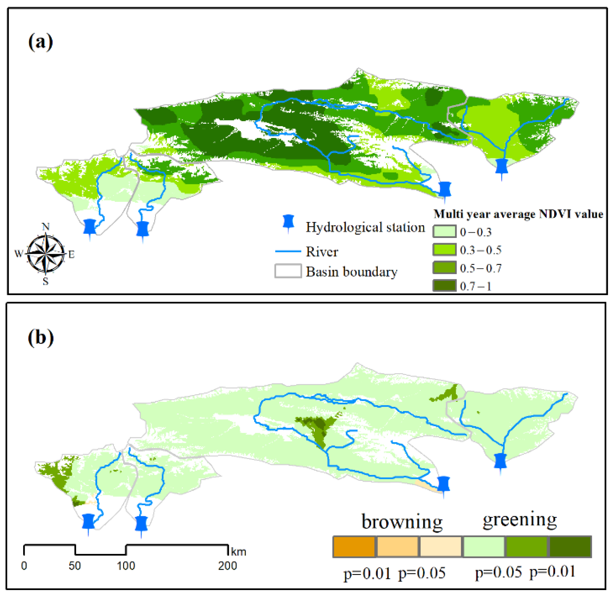
Multiyear average (a) and change trends (b) in NDVI values derived from GIMMS for the four basins during 1983−2012. p (browning) and p (greening) are the significance of the decrease and increase in NDVI values examined by the MK test. p values are divided into three levels: p < 0.01, 0.01 < p < 0.05, and p > 0.05.
Figure A2.
Multiyear average (a) and change trends (b) in NDVI values derived from GIMMS for the four basins during 1983−2012. p (browning) and p (greening) are the significance of the decrease and increase in NDVI values examined by the MK test. p values are divided into three levels: p < 0.01, 0.01 < p < 0.05, and p > 0.05.

Figure A3.
Downscaling of temperature at 2 m product in KDB.

Figure A4.
Flowchart of the parameter optimization base on genetic algorithm.

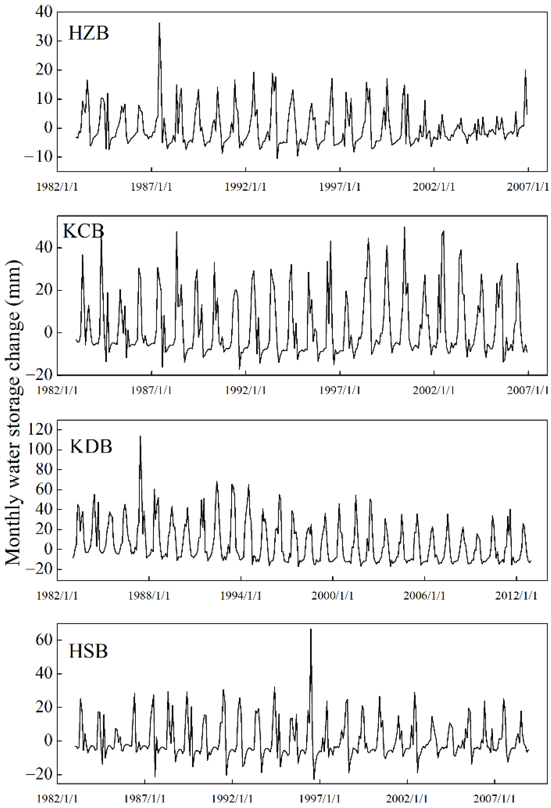
Figure A5.
Monthly water storage change of the four basins derived from the abcd model.

Figure A6.
Spatial (a) and temporal (b) Change trends in NDVI values derived from MODIS for the four basins during 2013−2021. p (browning) and p (greening) are the significance of the decrease and increase in NDVI values examined by the MK test. p values are divided into three levels: p < 0.01, 0.01 < p < 0.05, and p > 0.05.


Table A1.
Optimized parameters of abcd model.
| Basin | Periods | a | b (mm) | c | d (t − 1) | a1 | a2 |
|---|---|---|---|---|---|---|---|
| HZB | Pre-change | 0.92 | 248.92 | 0.31 | 0.12 | 15.96 | 9.17 |
| Post-change | 0.93 | 253.10 | 0.22 | 0.07 | 15.23 | 8.63 | |
| KCB | Pre-change | 0.86 | 267.12 | 0.36 | 0.25 | 21.23 | 10.84 |
| Post-change | 0.88 | 260.02 | 0.25 | 0.10 | 19.35 | 9.16 | |
| KDB | Pre-change | 0.99 | 311.30 | 0.10 | 0.33 | 52.10 | 11.28 |
| Post-change | 0.99 | 328.25 | 0.13 | 0.21 | 69.01 | 15.19 | |
| HSB | Pre-change | 0.89 | 301.26 | 0.17 | 0.12 | 17.29 | 6.09 |
| Post-change | 0.90 | 272.73 | 0.21 | 0.09 | 20.11 | 5.98 |
References
- Lian, X.; Piao, S.; Chen, A.; Huntingford, C.; Fu, B.; Li, L.Z.X.; Huang, J.; Sheffield, J.; Berg, A.M.; Keenan, T.F.; et al. Multifaceted characteristics of dryland aridity changes in a warming world. Nat. Rev. Earth Environ. 2021, 2, 232–250. [Google Scholar] [CrossRef]
- Huang, J.; Li, Y.; Fu, C.; Chen, F.; Fu, Q.; Dai, A.; Shinoda, M.; Ma, Z.; Guo, W.; Li, Z.; et al. Dryland climate change: Recent progress and challenges. Rev. Geophys. 2017, 55, 719–778. [Google Scholar] [CrossRef]
- Reynolds, J.F.; Stafford Smith, D.M.; Lambin, E.F.; Turner, B.L.; Mortimore, M.; Batterbury, S.P.J.; Downing, T.E.; Dowlatabadi, H.; Fernandez, R.J.; Herrick, J.E.; et al. Global desertification: Building a science for dryland development. Science 2007, 316, 847–851. [Google Scholar] [CrossRef] [PubMed] [Green Version]
- Haq, M.A. CDLSTM: A Novel Model for Climate Change Forecasting. Comput. Mater. Contin. 2022, 71, 2363–2381. [Google Scholar]
- Ghimire, S.; Yaseen, Z.M.; Farooque, A.A.; Deo, R.C.; Zhang, J.; Tao, X. Streamflow prediction using an integrated methodology based on convolutional neural network and long short-term memory networks. Sci. Rep. 2021, 11, 17497. [Google Scholar] [CrossRef]
- Brown, A.E.; Zhang, L.; McMahon, T.A.; Western, A.W.; Vertessy, R.A. A review of paired catchment studies for determining changes in water yield resulting from alterations in vegetation. J. Hydrol. 2005, 310, 28–61. [Google Scholar] [CrossRef]
- Budyko, M. Climate and Life; Academic Press: Cambridge, MA, USA, 1974. [Google Scholar]
- Arnold, J.G.; Srinivasan, R.; Muttiah, R.S.; Williams, J.R. Large area hydrologic modeling and assessment—Part 1: Model development. J. Am. Water Resour. Assoc. 1998, 34, 73–89. [Google Scholar] [CrossRef]
- Liang, X.; Lettenmaier, D.P.; Wood, E.F.; Burges, S.J. A simple hydrologically based model of land surface water and energy fluxes for general circulation models. J. Geophys. 1994, 99, 14415–14428. [Google Scholar] [CrossRef]
- Zhang, R.; Ouyang, Z.; Xie, X.; Guo, H.; Tan, D.; Xiao, X.; Qi, J.; Zhao, B. Impact of Climate Change on Vegetation Growth in Arid Northwest of China from 1982 to 2011. Remote Sens. 2016, 8, 364. [Google Scholar] [CrossRef] [Green Version]
- Zhang, S.; Yang, H.; Yang, D.; Jayawardena, A.W. Quantifying the effect of vegetation change on the regional water balance within the Budyko framework. Geophysics 2016, 43, 1140–1148. [Google Scholar] [CrossRef]
- Xing, W.; Wang, W.; Shao, Q.; Yong, B. Identification of dominant interactions between climatic seasonality, catchment characteristics and agricultural activities on Budyko-type equation parameter estimation. J. Hydrol. 2018, 556, 585–599. [Google Scholar] [CrossRef]
- Liang, W.; Bai, D.; Wang, F.; Fu, B.; Yan, J.; Wang, S.; Yang, Y.; Long, D.; Feng, M. Quantifying the impacts of climate change and ecological restoration on streamflow changes based on a Budyko hydrological model in China’s Loess Plateau. Water Resour. Res. 2015, 51, 6500–6519. [Google Scholar] [CrossRef]
- Liu, Q.; Yang, Z.; Han, F.; Wang, Z.; Wang, C. NDVI-based vegetation dynamics and their response to recent climate change: A case study in the Tianshan Mountains, China. Environ. Earth Sci. 2016, 75, 1189. [Google Scholar] [CrossRef]
- Wang, G.; Liu, G.; Li, C. Effects of changes in alpine grassland vegetation cover on hillslope hydrological processes in a permafrost watershed. J. Hydrol. 2012, 444, 22–33. [Google Scholar]
- Gan, G.; Liu, Y.; Sun, G. Understanding interactions among climate, water, and vegetation with the Budyko framework. Earth Sci. Rev. 2021, 212, 103451. [Google Scholar] [CrossRef]
- Shen, Y.; Shen, Y.; Guo, Y.; Zhang, Y.; Pei, H.; Brenning, A. Review of historical and projected future climatic and hydrological changes in mountainous semiarid Xinjiang (northwestern China), central Asia. Catena 2020, 187, 104343. [Google Scholar] [CrossRef]
- Chen, Y.; Li, W.; Deng, H.; Fang, G.; Li, Z. Changes in Central Asia’s Water Tower: Past, Present and Future. Sci. Rep. 2016, 6, 35458. [Google Scholar] [CrossRef]
- Shen, Y.; Shen, Y.; Fink, M.; Kralisch, S.; Chen, Y.; Brenning, A. Trends and variability in streamflow and snowmelt runoff timing in the southern Tianshan Mountains. J. Hydrol. 2018, 557, 173–181. [Google Scholar] [CrossRef]
- Zhang, M.; Wang, S. Precipitation isotopes in the Tianshan Mountains as a key to water cycle in arid central Asia. Sci. Cold Arid. Reg. 2018, 10, 27–37. (In Chinese) [Google Scholar]
- Liu, J.; Lawson, D.E.; Hawley, R.L.; Chipman, J.; Tracy, B.; Shi, X.; Chen, Y. Estimating the longevity of glaciers in the Xinjiang region of the Tian Shan through observations of glacier area change since the Little Ice Age using high-resolution imagery. J. Glaciol. 2020, 66, 471–484. [Google Scholar] [CrossRef] [Green Version]
- Mastrotheodoros, T.; Pappas, C.; Molnar, P.; Burlando, P.; Manoli, G.; Parajka, J.; Rigon, R.; Szeles, B.; Bottazzi, M.; Hadjidoukas, P.; et al. More green and less blue water in the Alps during warmer summers. Nat. Clim. Chang. 2020, 10, 155–161. [Google Scholar] [CrossRef]
- Han, J.; Gao, J.; Luo, H. Changes and implications of the relationship between rainfall, runoff and sediment load in the Wuding River basin on the Chinese Loess Plateau. Catena 2019, 175, 228–235. [Google Scholar] [CrossRef]
- Jian, S.; Zhao, C.; Fang, S.; Yu, K. Effects of different vegetation restoration on soil water storage and water balance in the Chinese Loess Plateau. Agric. For. Meteorol. 2015, 206, 85–96. [Google Scholar] [CrossRef]
- Wang, D. Evaluating interannual water storage changes at watersheds in Illinois based on long-term soil moisture and groundwater level data. Water Resour. Res. 2012, 48, W03502. [Google Scholar] [CrossRef]
- Huntington, T.G. CO2-induced suppression of transpiration cannot explain increasing runoff. Hydrol. Process. 2008, 22, 311–314. [Google Scholar] [CrossRef]
- Li, G.; Jiang, C.; Zhang, Y.; Jiang, G. Whether land greening in different geomorphic units are beneficial to water yield in the Yellow River Basin? Ecol. Indic. 2021, 120, 106926. [Google Scholar] [CrossRef]
- Wang, Z.; Qian, Y.; Zhang, H.; Huang, S.; Ji, H. Spatial distribution of soil physical-chemical properties in the region of the northern slopes of Karlike Range in East Tianshan Mountains to Naomaohu Basin. Arid Land Geogr. 2011, 34, 107–114. (In Chinese) [Google Scholar]
- Smith, W.K.; Dannenberg, M.P.; Yan, D.; Herrmann, S.; Barnes, M.L.; Barron-Gafford, G.A.; Biederman, J.A.; Ferrenberg, S.; Fox, A.M.; Hudson, A.; et al. Remote sensing of dryland ecosystem structure and function: Progress, challenges, and opportunities. Remote Sens. Environ. 2019, 233, 111401. [Google Scholar] [CrossRef]
- Matsushita, B.; Yang, W.; Chen, J.; Onda, Y.; Qiu, G. Sensitivity of the Enhanced Vegetation Index (EVI) and Normalized Difference Vegetation Index (NDVI) to topographic effects: A case study in high-density cypress forest. Sensors 2007, 7, 2636–2651. [Google Scholar] [CrossRef] [Green Version]
- Kumari, N.; Srivastava, A.; Dumka, U.C. A Long-Term Spatiotemporal Analysis of Vegetation Greenness over the Himalayan Region Using Google Earth Engine. Climate 2021, 9, 109. [Google Scholar] [CrossRef]
- Huete, A.R. A soil-adjusted vegetation index (SAVI). Remote Sens. Environ. 1988, 25, 295–309. [Google Scholar] [CrossRef]
- Marsett, R.C.; Qi, J.; Heilman, P.; Biedenbender, S.H.; Watson, M.C.; Amer, S.; Weltz, M.; Goodrich, D.; Marsett, R. Remote sensing for grassland management in the arid Southwest. Rangel. Ecol. Manag. 2006, 59, 530–540. [Google Scholar] [CrossRef]
- Huete, A.; Didan, K.; Miura, T.; Rodriguez, E.P.; Gao, X.; Ferreira, L.G. Overview of the radiometric and biophysical performance of the MODIS vegetation indices. Remote Sens. Environ. 2002, 83, 195–213. [Google Scholar] [CrossRef]
- Liu, S.; Wang, T.; Guo, J.; Qu, J.; An, P. Vegetation change based on SPOT-VGT data from 1998-2007, northern China. Environ. Earth Sci. 2010, 60, 1459–1466. [Google Scholar] [CrossRef]
- Zheng, L.; Xu, J.; Li, D.; Xia, Z.; Chen, Y.; Xu, G.; Lu, D. Increasing control of climate warming on the greening of alpine pastures in central Asia. Int. J. Appl. Earth Obs. 2021, 105, 102606. [Google Scholar] [CrossRef]
- Pu, Z.; Zhang, S. The effects of climate changes on the net primary productivity of natural vegetation in Tianshan Mountains. Pratac. Sci. 2009, 26, 11–18. (In Chinese) [Google Scholar]
- Huang, X.; Luo, G.; Wang, X. Land-Atmosphere Exchange of Water and Heat in the Arid Mountainous Grasslands of Central Asia during the Growing Season. Water 2017, 9, 727. [Google Scholar] [CrossRef] [Green Version]
- Fluet-Chouinard, E.; Lehner, B.; Rebelo, L.M.; Papa, F.; Hamilton, S.K. Development of a global inundation map at high spatial resolution from topographic downscaling of coarse-scale remote sensing data. Remote Sens. Environ. 2015, 158, 348–361. [Google Scholar] [CrossRef]
- Xie, X.; Li, A.; Jin, H.; Yin, G.; Bian, J. Spatial Downscaling of Gross Primary Productivity Using Topographic and Vegetation Heterogeneity Information: A Case Study in the Gongga Mountain Region of China. Remote Sens. 2018, 10, 647. [Google Scholar] [CrossRef] [Green Version]
- Xu, Z.; Han, Y.; Yang, Z. Dynamical downscaling of regional climate: A review of methods and limitations. Sci. China Earth Sci. 2019, 62, 365–375. [Google Scholar] [CrossRef]
- Stow, D.; Daeschner, S.; Hope, A.; Douglas, D.; Petersen, A.; Myneni, R.; Zhou, L.; Oechel, W. Variability of the seasonally integrated normalized difference vegetation index across the north slope of Alaska in the 1990s. Int. J. Remote Sens. 2003, 24, 1111–1117. [Google Scholar] [CrossRef]
- Hamed, K.H.; Rao, A.R. A modified Mann-Kendall trend test for autocorrelated data. J. Hydrol. 1998, 204, 182–196. [Google Scholar] [CrossRef]
- Pettitt, A.N. A non-parametric approach to the change-point problem. Appl. Stat. 1979, 28, 126–135. [Google Scholar] [CrossRef]
- Martinez, G.F.; Gupta, H.V. Toward improved identification of hydrological models: A diagnostic evaluation of the "abcd" monthly water balance model for the conterminous United States. Water Resour. Res. 2010, 46, W08507. [Google Scholar] [CrossRef]
- Xu, C.Y.; Seibert, J.; Halldin, S. Regional water balance modelling in the NOPEX area: Development and application of monthly water balance models. J. Hydrol. 1996, 180, 211–236. [Google Scholar] [CrossRef]
- Chang, F.; Chen, L. Real-Coded Genetic Algorithm for Rule-Based Flood Control Reservoir Management. Water Resour. Manag. 1998, 12, 185–198. [Google Scholar] [CrossRef]
- Liu, P.; Li, L.; Guo, S.; Xiong, L.; Zhang, W.; Zhang, J.; Xu, C. Optimal design of seasonal flood limited water levels and its application for the Three Gorges Reservoir. J. Hydrol. 2015, 527, 1045–1053. [Google Scholar] [CrossRef]
- Porporato, A.; Daly, E.; Rodriguez-Iturbe, I. Soil water balance and ecosystem response to climate change. Am. Nat. 2004, 164, 625–632. [Google Scholar] [CrossRef]
- Chen, X.; Alimohammadi, N.; Wang, D. Modeling interannual variability of seasonal evaporation and storage change based on the extended Budyko framework. Water Resour. Res. 2013, 49, 6067–6078. [Google Scholar] [CrossRef] [Green Version]
- Mu, Q.; Heinsch, F.A.; Zhao, M.; Running, S.W. Development of a global evapotranspiration algorithm based on MODIS and global meteorology data. Remote Sens. Environ. 2007, 111, 519–536. [Google Scholar] [CrossRef]
- Deng, Y.; Wang, S.; Bai, X.; Luo, G.; Wu, L.; Chen, F.; Wang, J.; Li, C.; Yang, Y.; Hu, Z.; et al. Vegetation greening intensified soil drying in some semi-arid and arid areas of the world. Agric. For. Meteorol. 2020, 292, 108103. [Google Scholar] [CrossRef]
- Zheng, L.; Xia, Z.; Xu, J.; Chen, Y.; Yang, H.; Li, D. Exploring annual lake dynamics in Xinjiang (China): Spatiotemporal features and driving climate factors from 2000 to 2019. Clim. Chang. 2021, 166, 36. [Google Scholar] [CrossRef]
- Fan, Y.; Sun, Z.; Wu, H.; Liu, X. Influences of fencing on vegetation and soil properties in mountain steppe. Pratac. Sci. 2009, 26, 79–82. (In Chinese) [Google Scholar]
- Di, S.; Li, Z.L.; Tang, R.; Pan, X.; Liu, H.; Niu, Y. Urban green space classification and water consumption analysis with remote-sensing technology: A case study in Beijing, China. Int. J. Remote Sens. 2019, 40, 1909–1929. [Google Scholar] [CrossRef]
- Zhang, H.F.; Li, X.; Wang, J.G.; Yang, Y.J. The structure characteristic of the plant community in the lower reaches of Tarim River. Ecol. Environ. 2007, 16, 1219–1224. (In Chinese) [Google Scholar]
- Wu, X.Q.; Meng, J.J. The Land Use/Cover Changes and the Eco-environmental Responses in the Lower Reaches of Tarim River, Xinjiang. Arid. Zone Res. 2004, 1, 38–43. (In Chinese) [Google Scholar]
Figure 1.
Location of study area and the representative vegetation landscape. The subfigure (a) shows the location of Tianshan Mountains in the world; the subfigure (b) shows the basic geographic information of the four basins; the subfigures (c–f) show the NDVI values under different landscape types.

Figure 2.
Schematic of extended Budyko decomposition method to quantify the climate and underlying surface changes impacts on streamflow change at seasonal scale. Changes from Point A to B indicate the relation between evaporation ratio and climate condition under the influence of climate change. Changes from Point A to C indicate the relation between evaporation ratio and climate condition under joint influences from climate and underlying surfaces changes.

Figure 3.
Phenological curve of the four basins based on regional mean NDVI from 1980 to 2012. Dashed lines indicate that vegetation of the four basins complete the “green up” processes in June and start to wither after September.
Figure 3.
Phenological curve of the four basins based on regional mean NDVI from 1980 to 2012. Dashed lines indicate that vegetation of the four basins complete the “green up” processes in June and start to wither after September.

Figure 4.
Annual variation of summer maximum NDVI derived from GIMMS for the four basins during 1983−2012. Change trends of NDVI have been determined by linear least-squares regression and the Mann–Kendall test.
Figure 4.
Annual variation of summer maximum NDVI derived from GIMMS for the four basins during 1983−2012. Change trends of NDVI have been determined by linear least-squares regression and the Mann–Kendall test.

Figure 5.
Variations of annual and summer streamflow of the four basins. Change trends of annual and summer streamflow have been determined by linear least-squares regression and the Mann–Kendall test.
Figure 5.
Variations of annual and summer streamflow of the four basins. Change trends of annual and summer streamflow have been determined by linear least-squares regression and the Mann–Kendall test.

Figure 6.
Simulated streamflow by abcd model in the four basins for pre-change period and post-change period.
Figure 6.
Simulated streamflow by abcd model in the four basins for pre-change period and post-change period.

Figure 7.
Quantification results of the climate-induced and underlying surface-induced changes in streamflow for the four basins during summer periods.
Figure 7.
Quantification results of the climate-induced and underlying surface-induced changes in streamflow for the four basins during summer periods.

Figure 8.
Quantification results of the climate-induced and underlying surface-induced changes in streamflow for the four basins during each summer month.
Figure 8.
Quantification results of the climate-induced and underlying surface-induced changes in streamflow for the four basins during each summer month.

Table 1.
Performance (NSE value) of abcd model for monthly streamflow simulation.
| Basin | Pre-Change | Post-Change | ||
|---|---|---|---|---|
| Calibration | Validation | Calibration | Validation | |
| HZB | 0.78 | 0.83 | 0.71 | 0.79 |
| KCB | 0.78 | 0.71 | 0.75 | 0.72 |
| KDB | 0.85 | 0.76 | 0.83 | 0.80 |
| HSB | 0.86 | 0.91 | 0.89 | 0.90 |
Table 2.
Values of climatic and hydrological variables in HZB, KCB, KDB, HSB during summer (June to September).
Table 2.
Values of climatic and hydrological variables in HZB, KCB, KDB, HSB during summer (June to September).
| Basin Name | Area (km2) | Periods | Coefficient of Elasticity | ||||||
|---|---|---|---|---|---|---|---|---|---|
| HZB | 3342 | 1983−2006 | 273.03 | 561.02 | 62.17 | 1.29 | 1.96 | −0.96 | −1.57 |
| KCB | 2946 | 1983−2006 | 226.05 | 397.75 | 119.75 | 0.69 | 1.36 | −0.36 | −0.87 |
| KDB | 18,827 | 1983−2012 | 166.20 | 431.33 | 105.42 | 0.49 | 1.22 | −0.22 | −0.79 |
| HSB | 4311 | 1983−2008 | 173.78 | 450.99 | 50.81 | 0.97 | 1.70 | −0.70 | −1.45 |
Publisher’s Note: MDPI stays neutral with regard to jurisdictional claims in published maps and institutional affiliations. |
© 2022 by the authors. Licensee MDPI, Basel, Switzerland. This article is an open access article distributed under the terms and conditions of the Creative Commons Attribution (CC BY) license (https://creativecommons.org/licenses/by/4.0/).
Share and Cite
MDPI and ACS Style
Zheng, L.; Xu, J.; Chen, Y.; Wu, Z. Increasing Streamflow in Poor Vegetated Mountain Basins Induced by Greening of Underlying Surface. Remote Sens. 2022, 14, 3223. https://doi.org/10.3390/rs14133223
AMA Style
Zheng L, Xu J, Chen Y, Wu Z. Increasing Streamflow in Poor Vegetated Mountain Basins Induced by Greening of Underlying Surface. Remote Sensing. 2022; 14(13):3223. https://doi.org/10.3390/rs14133223
Chicago/Turabian StyleZheng, Lilin, Jianhua Xu, Yaning Chen, and Zhenhui Wu. 2022. "Increasing Streamflow in Poor Vegetated Mountain Basins Induced by Greening of Underlying Surface" Remote Sensing 14, no. 13: 3223. https://doi.org/10.3390/rs14133223
Note that from the first issue of 2016, this journal uses article numbers instead of page numbers. See further details here.