
Spatiotemporal Variations of Forest Vegetation Phenology and Its Response to Climate Change in Northeast China


1
School of Forestry, Northeast Forestry University, Harbin 150040, China
2
Key Laboratory of Sustainable Forest Ecosystem Management-Ministry of Education, Northeast Forestry University, Harbin 150040, China
*
Author to whom correspondence should be addressed.
Remote Sens. 2022, 14(12), 2909; https://doi.org/10.3390/rs14122909
Submission received: 29 April 2022
/
Revised: 2 June 2022
/
Accepted: 16 June 2022
/
Published: 17 June 2022
(This article belongs to the Special Issue Monitoring Forest Carbon Sequestration with Remote Sensing)
Abstract
:Vegetation phenology is an important indicator of vegetation dynamics. The boreal forest ecosystem is the main part of terrestrial ecosystem in the Northern Hemisphere and plays an important role in global carbon balance. In this study, the dynamic threshold method combined with the ground-based phenology observation data was applied to extract the forest phenological parameters from MODIS NDVI time-series. Then, the spatiotemporal variation of forest phenology is discussed and the relationship between phenological change and climatic factors was concluded in the northeast China from 2011 to 2020. The results indicated that the distribution of the optimal extraction threshold has spatial heterogeneity, and the changing rate was 3% and 2% with 1° increase in latitude for SOS (the start of the growing season) and EOS (the end of the growing season). This research also notes that the SOS had an advanced trend at a rate of 0.29 d/a while the EOS was delayed by 0.47 d/a. This variation of phenology varied from different forest types. We also found that the preseason temperature played a major role in effecting the forest phenology. The temperature in winter of the previous year had a significant effect on SOS in current year. Temperature in autumn of the current year had a significant effect on EOS.
1. Introduction
Vegetation phenology is the subject which studies the cyclical events throughout the whole life of plants and how these events respond to environmental changes [1]. Lots of studies have clarified that global warming, with the consequence of greenhouse gases increasing, has significantly shifted the vegetation phenology in terrestrial ecosystems of the Northern Hemisphere [2,3], and the variation of vegetation phenology has greatly impacted the terrestrial ecosystem functions and structures [4,5]. Previous researches have concluded that the forest ecosystem is the main part of terrestrial ecosystem in the Northern Hemisphere, such as in China [6], America [7], Canada [8], and Europe [9], and plays an important role in the global carbon balance. Vegetation phenology may also feed back to climate changes, for example, the prolonged length of growing season (LOS) could affect the ability of forest carbon sequestration and mitigate the global temperature increase [10]. Therefore, studying the relationship of vegetation to climate is essential for enhancing the vegetation productivity, carbon storage and carbon cycle of the terrestrial ecosystem.
Phenology research dates back to ancient agricultural times. People originally obtained the timing of phenological events by observing and establishing phenology observation networks, which has been occurring since the 18th century [11]. Previous studies indicate that the spring phenological variation of most vegetation had an advanced trend proven by ground-based observations during the past decades in Northern Hemisphere. Menzel et al. concluded that the average advance of spring was 2.5 days per decade in 21 European countries between 1921 and 2000 [12]. Keenan et al. found that the temperate forest over the eastern US had a strong trend of earlier springs over combined long-term ground observations of phenology [13]. Rosbakh et al. analyzed the 67 common plant species in Siberia and found that boreal forest springs advanced 2.2 days per decade, while leaf senescence was delayed at a rate of 1.6 days per decade during 1976–2018 [14]. However, ground-based observation only recorded the timing of phenological events for species, so that it is difficult to clearly understand the seasonal changes of vegetation phenology on a regional or global scale [1]. During the past few years, remote sensing technology developed rapidly, which, as a new tool, overcomes the above limitations of ground-based observation. Data obtained from satellite remote sensing could obtain the spatially continuous information of surface, which had increasingly been used in the studying and monitoring of vegetation phenology, such as vegetation index (VI), which is a combination of two or more wavelength ranges of surface reflectance to enhance characters or details of vegetation [15]. The more commonly used remote-sensing vegetation indices include the normalized differential vegetation index (NDVI) [16], the enhanced vegetation index (EVI) [17], and the leaf area index (LAI), which is a forest structure parameter and can also be used to extract forest vegetation phenology [18].
Based on satellite data, the changes of vegetation dynamics can be studied using the vegetation indices or biophysical variables time series [19]. The quality of long-term series remote sensing data would make a big difference for the calculation of the surface vegetation phenology. Due to cloud contamination, atmospheric variability, and bi-directional effects, the long-term series remote sensing data still have a lot of noise [20]. To extract the spectral–temporal signatures accurately, many methods have been developed for reducing noise to construct high-quality VI time-series, and these can be classified into three categories: empirical methods, data transformations, and curve fitting methods [15]. The empirical methods are easy to apply, but they are determined by empirical parameters, such as the length of the sliding window. Data transformation methods use the mathematical manipulation to decompose time-series curves into seasonal, cyclical, trend, and irregular components [21], while the performance is poor in smoothing the irregular or asymmetric data [15]. Curve fitting methods fit the VI time-series to a particular function by utilizing least squares, with the advantage of effectively reducing the noise and no empirical constraints [15]. Logistic function, asymmetric Gaussian functions, and the Savitzky–Golay (S-G) filter are commonly used methods. Lara et al. compared the three smoothing methods included in TIMESAT software and concluded that the S-G filter had better performances [22]. Once the time-series curves based on remote sensing data were reconstructed, phenological parameters could be extracted.
The identify the method of the vegetation phenology from remote sensing time-series included inflection points and relative thresholds [23,24]. The inflection point method uses the inflection point of the VI time-series curve to identify the SOS (The start of the growing season) or EOS (The end of the growing season). The inflection point phenology detection algorithm usually uses a logistic function to fit the VI time-series and the results of the inflection point method relied more on the shape of the VIs time-series and the accuracy of the extracted phenology, which varied through the with and without filtering steps [25]. For the relative threshold method, the SOS or EOS was determined with a predefined percentage of VI amplitude, such as 20%, 30%, or other values [26]. Therefore, determining the relative thresholds was quite important to estimate vegetation phenological events. Wang et al. took 50% of maximum NDVI value as the threshold to extract the SOS and EOS and accessed the spatio-temporal trends of vegetation phenology, which showed dramatic spatial heterogeneity with different rates during the 1982–2012 [27]. Ding et al. found that the extraction of phenological events by using 20% of the annual NDVI amplitude was highly consistent with ground-based observation data on the Tibetan Plateau from 1982 to 2012 [28]. Xu et al. first used the fixed threshold method to extract the phenology in Tibet Plateau based on the remote sensing. The results showed that the SOS has an obvious overestimation, with about 50% error of estimation (RMSE > 50). Combined with the EC flux measurements, the SOS and EOS value of the threshold method were determined with the value of 0.17 and 0.2 in the grasslands of Inner Mongolia, while these were 0.14 and 0.29 in Tibet Plateau of China [29]. Yu studied the vegetation phenology changes of northeast of China with a threshold method and threshold of 0.2 was used in this study [30]. However, a study of phenology in the same area with a threshold of 0.3 was used in Zhao’s research [31]. Fu et al. studied the effect of autumn phenology in the Greater Khingan Mountains of northeastern China, and a threshold of 0.3 was used [32]. This research area was obviously smaller, but the same value was used to extract the SOS, EOS, and LOS from the remote sensing data. Considering the spatial heterogeneity of the vegetation, the extracted phenology of the vegetation across diverse ecosystems and at different scales from satellite data might have significant differences using the fixed-threshold method. In addition, the fixed-threshold method was sensitive to non-vegetation-related variations in the VI time series, and it led to a considerable error in the phenology metrics by using remote sensing data [15]. Furthermore, it might increase the uncertain error in phenology research. Therefore, it is essential to develop a new method of threshold determination to increase the accuracy of the extracted phenological parameters.
Plant growth has been associated with temperature and precipitation to implicate climate trends in phenology shifts [33]. In turn, climate change has significantly affected vegetation phenology, which further changes the carbon, water, and energy exchange between the terrestrial ecosystem and atmosphere. Wolf et al. found that a warmer spring and earlier vegetation activity has a positive effect on the carbon cycle [34]. Xu et al. concluded that warming induced earlier greening in the Northern Hemisphere during 1982–2011 [35]. The temperature changes the activity of enzymes, and the increase in temperature can promote the activity of enzymes to accelerate vegetation phenology. Jeong et al. concluded that the warming temperature enhances vegetation photosynthesis and prolongs the LOS by advancing the SOS and delaying the EOS [36]. Liu et al. found that the warming climate prolonged the LOS of plants in the Northern Hemisphere by using the GIMMS NDVI3g [37]. Zhao et al. pointed out that over the past decades, the EOS has been delayed by 0.13 days each year in northeastern China [31]. Wang et al. discovered an advanced SOS and a delayed EOS by utilizing remote-sensing data and climate data in the northeastern China from 2011 to 2019 [38]. In addition, precipitation is also a factor which effects the phenology. Piao et al. found that precipitation played a significant role in effecting the summer NDVI in Eurasia [39]. Cong et al. found that increasing precipitation could result in the advanced SOS of broad-leaf forests in northern China by using the GIMMS NDVI3g [40]. It is not difficult to conclude from the existing research that the vegetation growth environment varies across the regions, and the response of phenology to meteorological factors is different [41]. Although the relationship between temperature and precipitation and vegetation phenology has been discussed, these are complex responses that vary according to the spatial heterogeneity of the vegetation. Therefore, it is necessary to demonstrate the relationship between the phenology and the factors of preseason, interannual, and multi-climatic factors and to conduct a comprehensive study on interactions that exist between the SOS and EOS.
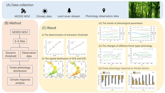
In this study, we developed a dynamic thresholds method combining MODIS NDVI time-series and ground-based observation data to extract the vegetation phenological parameters in Northeast China from 2011–2020. We analyzed the changing characteristics of phenology of different forest types in northeast China during the last decade. We aimed to (1) develop a suitable dynamic threshold method to extract the SOS and EOS, combining MODIS NDVI time-series and ground-based phenology observation data; (2) summarize the spatial and temporal changing characteristics of the phenology of different forest types in northeast China; (3) study the relationship and interaction between the phenology of different forest types and climate factors on a regional scale.
We hope that this study can provide a reference to further clarify the relationship between the phenology of the different forest vegetation types and climate factors and the interaction against the backdrop of global warming.
2. Materials and Methods
2.1. Study Area
The research area of this study is the Northeast China (NEC), which includes the Heilongjiang, Jilin, and Liaoning provinces, is located from 118°50′ E to 135°09′ E and 38°42′ N to 53°35′ N (Figure 1) [42]. NEC has the considerable climatic and topographical gradients, and the main topography of NEC is mountains and plains, with mountains in the east, west and north, and plains in the middle and south [43]. Due to geographical location NEC belongs to a temperate continental monsoon climate [44], which is divided into a warm temperate zone, temperate zone, and cold temperate zone from south to north and has obvious differences in humidity from east to west [45]. As a result, NEC has a unique vegetation distribution and is one of the regions most sensitive to global change [46]. NEC has one of the largest natural forests in China, which are mainly scattered throughout the Changbai Mountains, Lesser Khingan Mountains, and Greater Khingan Mountains. The main vegetation types of NEC forests are cold-temperate deciduous coniferous forests, deciduous broad-leaved forests, and mixed coniferous broad-leaved forests. Therefore, as a main part of the boreal forest ecosystem, NEC is an ideal region for researching the forest–climate relationships of northeastern Asia.
2.2. Materials
2.2.1. MODIS NDVI Dataset
The NDVI was obtained from a moderate-resolution imaging spectroradiometer (MODIS) provided by the National Aeronautics and Space Administration (NASA). Available online: https://search.earthdata.nasa.gov (accessed on 23 April 2022). MOD13Q1 (MODIS/Terra Vegetation Indices 16-Day L3 Global 250 m SIN Grid) was used in this study. The time span of the data is from 1 January 2011 to 31 December 2020. A total of 1150 images were downloaded. The spatial resolution of the NDVI data products is 250 m, and the temporal resolution is 16 days [20]. The NDVI calculation is a combined operation between the red spectral band (Red) and near-infrared spectral band (NIR) as follows [47]:
where NIR is the reflectivity values in the near infrared band and Red is the reflectivity of the red band. The value range of NDVI is from −1 to 1.
ArcGIS software and MRT (Modis Reprojection Tool) were used to process the downloaded images. Image preprocessing included reprojection, cutting, splicing, and so on.
The software TIMESAT, which contains a S-G filter, asymmetrical Gaussian (AG) function fitting, and double logistic function fitting, was employed to reduce the noise and smooth the NDVI time-series [48]. In this study, the S-G filter, which is a weighted moving average filter proposed by Savitzky and Golay [49], was chosen for smoothing the NDVI time-series because of its better performance.
The weight of the S-G filter depends on the polynomial least squares fit in the filter window [50]. The general equation of the S-G filter for NDVI time-series smoothing can be given as follows [51]:
where represents the original value of the i-th NDVI at time j, represents the resultant NDVI value, Ci represents the coefficient for the i-th NDVI value of the filter, and m represents the half-width of the smoothing window.
2.2.2. Meteorological Data
The meteorological data used in this study are the Global Summary of the Day data provided by the National Oceanic and Atmospheric Administration (NOAA). Available online: https://www.ncei.noaa.gov/data/global-summary-of-the-day (accessed on 23 April 2022). First, we downloaded the daily average temperature and daily cumulative precipitation data from stations throughout the NEC and surrounding areas from 2011 to 2020. In order to maintain the continuity and effectiveness of the data, we downloaded the data from the stations of research area and around research area and deleted the stations with more than 5% of missing data and obtained 116 stations through quality control; the statistical information can be found in Table 1. Subsequently, we converted the daily data to annual data and seasonal data, that is, spring (March–May), summer (June–August), autumn (September–November), and winter (December–February (of the next year)). Finally, we obtained the interpolation grid, which had a consistent spatial resolution with the spatial resolution of NDVI, by applying the simple kriging interpolation method.
2.2.3. Land Cover Dataset
It is very crucial to distinguish between vegetation and non-vegetation by using land cover data, specifically in the extraction of vegetation phenology. In this study, the land cover data FROM-GLC (Finer Resolution Observation and Monitoring of Global Land Cover, FROM-GLC), developed by group Pro. Peng Gong at Tsinghua University, was used. FROM-GLC data is a global land cover map at 30 m resolution obtained by using Landsat TM and ETM+ data with high accuracy. Available online: http://data.ess.tsinghua.edu.cn (accessed on 23 April 2022). In this study, all forest types were reclassified into coniferous forest (CF), broadleaf forest (BF), and mixed forest (MF).
2.2.4. Phenology Observation Data
In this study, we downloaded the phenology observation data from the Chinese Phenological Observation Network (CPON). Available online: http://www.geodata.cn (accessed on 23 April 2022). The phenology observation data were used to determine the threshold of the NDVI time-series and evaluate the accuracy of phenological parameters extracted by using the NDVI time-series. Eight stations in NEC were selected; these were Nenjiang, Dedu, Jiamusi, Harbin, Mudanjiang, Changchun, Shenyang, and Gaizhou stations. Combined with the geographical location of the phenological observation sites, the statistical information of the measured data after sorting can be found in Table 2.
Descriptions of the datasets applied in our study are shown in Table 3.
2.3. Method
2.3.1. Method of the Vegetation Phenology Extraction
In this study, the dynamic threshold method, also called the proportional threshold method, was used to extract SOS and EOS from NDVI time-series processed by a S-G filter. The point in time when NDVI increases to a certain percentage of the NDVI amplitude of the year is defined as the SOS, and the time when NDVI decreases to a certain percentage of the NDVI amplitude of the year is defined as the EOS (Figure 2). The threshold used in this method is not a specific vegetation index value but a dynamic ratio form, compared with the absolute threshold and difference threshold; the dynamic threshold method has better applicability in both the time and space domain [48]. The principle of this method is as follows:
The calculation formula of vegetation phenology extracted by the dynamic threshold method as follows [52]:
where PS and PE represent the extraction threshold corresponding to the SOS and EOS, respectively. NDVISOS and NDVIEOS are the corresponding NDVI values when SOS and EOS occurred. NDVImax represents the maximum NDVI during the whole time-series, NDVImin(left) is the minimum NDVI of the first half of the time-series, and NDVImin(right) is the minimum NDVI of the second half of the time-series.
Firstly, we selected representative tree species in each phenological observation site and calculated the mean DOY of leaf onset and leaf senescence as SOS and EOS, respectively.
Secondly, we extracted the corresponding remote-sensing pixels of the eight phenology observation stations selected and calculated the mean NDVI of each pixel as the phenological parameters to extract the original data. Then, we brought the NDVI corresponding to the occurrence day of the observation-based phenological parameters into Formulas (3) and (4), and thus the optimal extraction threshold of each station was able to be calculated.
Thirdly, we assumed that the functional relationship between the optimal extraction threshold P of the vegetation phenology at different latitudes and latitude L as follows:
where , which represents the optimal extraction threshold set corresponding to the eight phenology observation stations; , which represents the latitude set of the eight phenology observation stations. The values of coefficients A and B were obtained by fitting with the least square method, and the functional relationship between the optimum extraction threshold and latitude of vegetation phenology was established.
Finally, the optimal extraction threshold for each pixel can be calculated based on the central latitude value of each pixel by using the relationship established in Formula (5), and the phenological parameter can be extracted using this threshold.
2.3.2. Analysis Method
Statistical analysis is one of the most commonly used data analysis methods and is widely used in empirical modeling and the accuracy assessment of remote sensing research [53]. This parametric statistical technique requires that the data follows a continuous and normal distribution [54]. Therefore, the normal distribution test should be performed first. The data used in the study all followed the normal distribution. After that, a linear relationship between the forest phenology of different forest types and the latitude, year, and climatic factors were fitted by using the least squares method, and the changing rate of forest phenology affected by latitude, year, and climatic factors was analyzed by comparing the slope of the fitted linear function (Figure 3).
When x increases ∆x, y increases with the increase in x, but the changes in the ∆y are varied, according to the fitting function. This difference was determined by the slope of the linear function. So, when x increases ∆x, the ∆y2 is larger than ∆y1 in Figure 3. Therefore, the slope of the linear function can satisfy the necessity of comparing the changing rate of forest phenology affected by latitude, year, and climatic factors.
Then, the correlation coefficient was selected to explore the relationship between forest phenology and climatic factors. The correlation coefficient was calculated as follows [55]:
where R represents correlation coefficient between X and Y, n represents the number of samples, X and Y represent the values in the i-th year, and and represent the average of values of all years, respectively. The values of range from 0 to 1, which is larger, meaning that the correlation relationship is stronger between two variables. In addition, we used the p-value to test the significance of the correlation coefficient.
To analyze the association between the forest phenology and climatic factors and the partial correlations of the forest phenology and monthly temperature, precipitation was calculated as follows [56]:
where rab[c] represents the partial correlation coefficient between phenological parameter a and climatic variable b when climatic variable c was controlled; and rab, rac, and rbc represent the liner correlation coefficient between each other, respectively. n represents the number of samples and m represents the number of independent variables.
2.3.3. Validation
In this study, the determination coefficient (R2), root mean squared error (RMSE), and mean absolute percentage error (MAPE) were selected to evaluate model accuracy. The equations are shown as follows [55]:
where is the measured values and is the predicted values for the sample , is the average of all the samples, and is the number of samples.
3. Results
3.1. Determination of the Dynamic Threshold for Vegetation Phenology
In this study, the relationship between the optimal extracted threshold and the latitude of forest phenology remote-sensing based in northeast China was determined by using the S-G filter and dynamic threshold method, which was combined with NDVI time-series data and ground phenology observation data. Due to the lack of phenological observation data from stations, only eight points in 2014 was simultaneous and available during the research period. The scattering plot between the extracted threshold and latitude can be found in Figure 4. This figure showed that there was a significant relationship between the extracted threshold and latitude. Figure 4a showed the relationship between the optimal extracted threshold of SOS (PS) and latitude. A least square method was used to fit the function. The fitted function was defined as followed.
where PS is the threshold to determine the SOS from NDVI time-series data. L is the latitude. The R2, RMSE, and MAPE of the fitted model are 0.9589, 0.0245, and 6.617%, respectively. The models and the coefficients all passed the significance test at a 95% level of significance.
The linear relationship between the optimal extracted threshold of EOS (PE) and latitude was also significant, and the fitting function is showed in Equation (12).
where PE is the threshold to determinate the EOS from NDVI time-series data. L is the latitude. The R2, RMSE, and MAPE of the fitted model are 0.9421, 0.0185, and 4.511%, respectively. The model and the coefficient passed the significance test at a 95% level of significance.
Then we evaluated the accuracy of the phenology extracted by using the fixed thresholds of 20% [28], 30% [31], and 50% [27] used by other scholars and dynamic threshold method developed in this study. The RMSE and MAPE between the estimated and measured SOS were calculated, and the results are shown in Table 4. The phenology extracted by using the dynamic threshold method has a better accuracy than the fixed threshold method with a RMSE and MAPE of 11.875 d and 7.623% for SOS and 9.012 d and 2.44% for EOS, respectively. However, the fixed threshold method, with the values of 20%, 30%, and 50%, had lower accuracy. The fixed threshold with the value of 20% has the larger error than other methods. The RMSE is 30.182 d for SOS and 34.846 d for EOS, and this brings the estimated error to about one month. Followed by the fixed threshold with the value of 30% with the RMSE and MAPE of 26.716 d and 16.118% for SOS and 26.528 d and 8.373% for EOS, respectively. Compared with other three methods, the fixed threshold with the value of 50% has a middling level of error, but the error is about 19 d for SOS, and for EOS and MAPE it is 14.723% and 6.118%, respectively.
The scattering plots between measured and extracted phenology using fixed and dynamic threshold methods are shown in Figure 5. For SOS, the extracted SOS using fixed threshold has an obvious bias from the measured SOS. SOS was underestimated for the fixed threshold of 20%. By contrast, SOS was overestimated for the fixed threshold of 30% and 50%. Extracted EOS using a fixed threshold had an obvious overestimating phenomenon. It indicates that the fixed threshold method increases the estimating error and increases the uncertain error in extracted phenology analysis.
3.2. Characteristics of Forest Phenology in the Northeast China
3.2.1. Spatial Distribution of the Forest Phenology
The characteristics of forest phenological variation in the northeast China from 2011 to 2020 were analyzed. The spatial pattern of the mean forest SOS in NEC from 2011 to 2020 is shown in Figure 6. The variation of the forest SOS showed significant spatial heterogeneity in the study area. The spatial distribution of the mean SOS exhibited a correlation with the latitude as the southern part was earlier than the northern part. The mean SOS in the NEC primarily occurred between 95th and 135th day, which accounted for 83.46% of the study area, and the average of the SOS in the whole research area was 116 days. The forest located 45 degrees south of the northern latitude had an earlier SOS, between the 95th and 105th day, whereas the area with an average SOS later than 135 days was mostly located in the northernmost Greater Khingan Mountains, which principally distributed in the CF and had a lower temperature. Factors leading to this spatial distribution of SOS were not only related to temperature but also to the type of tree species, because the south of NEC was dominated by broadleaf and mixed forest, while the north of NEC was dominated by coniferous and mixed forests (see Figure 1).
The mean EOS were mainly in ranges of 300 days to 330 days, which is late October and late November, and the average EOS was 315th days in the northeastern China (Figure 7). The characteristics of the forest EOS in the northeastern China from 2011 to 2020 also had obvious heterogeneity. From the northwest to the southeast of the study area, the average of the EOS was gradually delayed, which showed significantly variation according to the latitude. The forest in the southeastern Changbai Mountains, near the coast, had relatively late EOS dates, while the EOS in the northernmost Greater Khingan Mountains were earlier.
The average LOS gradually lengthened from north to south (Figure 8). The average of the LOS was mainly in ranges of 150 days to 230 days with the counting of pixels for 85.28%. The average LOS in the study area was 199 days. The LOS was longer in coastal areas at low latitudes in the east of Liaoning Province. The regions with the LOS greater than 230 days were mainly distributed in the south of 43° N and east of 122° E, accounting for 9.84% of the research area. The shortest LOS was less than 150 days in the middle of the Greater Khingan Mountains in the Heilongjiang Province.
Long-term variations of phenology could reflect the state of vegetation grown. In order to explore the relationship between forest phenological changes and latitudes in NEC from 2011 to 2020, we divided the study area into 15 parts by 1 degree latitude and calculated the average forest phenological parameters for each part. The results can be found in Figure 9. The results indicated that the SOS of the forest was sightly delayed with the increase of latitude, and the SOS was delayed by 2.33 days per latitude with the increase in latitude. The event of forest EOS would shift to an earlier time with the increase of latitude, and EOS increased by 2.22 days per latitude with the increase of latitude. The LOS of forest decreased with increasing latitude, and LOS decreased by 4.55 days per latitude with increase in latitude.
3.2.2. The Interannual Variability and Trends of Forest Phenology
Forest phenology fluctuated significantly in NEC from 2011 to 2020 and the interannual variation trend was obvious (Figure 10). The SOS of forest phenology showed a weak advancing trend of approximately 0.29 d/a. The EOS showed a weak delayed trend with a rate of 0.47 d/a. Figure 10 also showed that the variation range of LOS was larger, followed by the EOS and SOS. Overall, the LOS displayed sizeable increases of approximately 0.76 d/a. These trends may be related to global warming because the rising temperature advanced the spring and the cooling temperature trend delayed in the autumn.
3.3. The Variation and Trends of Phenology in Different Forest Types
3.3.1. The Spatial Distribution of Phenology in Different Forest Types
In order to investigate whether the phenological characteristics of the different forest types changed with latitudes, we calculated the average phenological parameters of three forest types at different latitudes and analyzed and compared the results. The results showed that all three parameters of different forest types showed fluctuations with different ranges. As per the findings, the following can be discerned (Figure 11): as the latitude increased, the SOS tended to delay. It can clearly be seen that the sensitivity of BF and MF to latitude changes were significantly higher than CF. The SOS of the MF was delayed by approximately 2.51 days per latitude, while the SOS of CF delayed 1.70 days per latitude. The SOS of BF was showed a largest delaying trend with a rate of 2.68 days per latitude.
The EOS of different forest types showed a significant delayed trend with the increase in the latitude (Figure 12). The EOS of BF was the greatest significant with a rate of 2.65 days per latitude. Followed by MF, the changing rate of the EOS of MF was 2.47 days per latitude. The CF had the smallest changing rate of 2.0 days per latitude, compared with other two forest types.
The variation range of LOS was affected by the EOS and SOS. The LOS of different forest types showed a significant decreasing trend with the increase of latitude (Figure 13). The LOS of BF had the greatest changing rate of 5.33 days per latitude. The LOS of MF was 4.98 days per latitude, and the CF had the smallest changing rate of 3.69 days per latitude, compared with other two forest types.
3.3.2. The Interannual Variation and Trends of Forest Phenology in Different Forest Type
The annual variation of phenology in different types of forest from 2011 to 2020 can be found in Figure 14. The SOS of all three forest types demonstrated an advancing trend year by year in the study area. The MF had the most obvious trend of advance with the rate 0.45 days per year and changing rate of BF was 0.28 days per year. While the CF changed weakly with 0.20 days per year.
All forest types had delayed EOS, whereas MF exhibited the most considerable EOS of all with the rate of 0.58 days per year (Figure 15). The interannual changing rate of EOS of the CF was 0.46 days per year. The EOS changing rate of MS was weaker than other two forest types with a rate of 0.32 days per year.
The variation of LOS displayed an extended trend due to the combined effect of SOS and EOS, and the annual change rate of all was greater than 0.6 days per year, with the most specific change range was BF, followed by MF and CF (Figure 16). The interannual changing rate was 0.86, 0.77 and 0.66 days per year.
3.4. Effects of Climate Factors on Forest Phenology in the Northeast China
3.4.1. Effects of Precipitation on the Forest Phenology
Affected by geographical and climatic factors, there are significant differences in the precipitation and temperature in different regions of the NEC from 2011 to 2020. The maximum difference in the annual cumulative precipitation is 500 mm. As shown in Figure 17, the SOS had a significant correlation with the annual cumulative precipitation (P < 0.01). With the increase of precipitation, the phenology of forests showed a trend of advanced SOS and delayed EOS, which extended the LOS. The response of the three phenological parameters to the annual cumulative precipitation from large to small was LOS, EOS, and SOS. The SOS advanced 2.9 days per 100 mm, while the EOS and LOS delayed 4.3 days per 100 mm and 7.1 days per 100 mm, respectively.
In this study, we analyzed the response of different forest phenological parameters to annual cumulative precipitation (Figure 18). The SOS in the BF area was obviously correlated with annual cumulative precipitation at a rate of advanced 3.7 d/100 mm (P < 0.05). With the increase in annual cumulative precipitation, the EOS of all forest types tended to delay, and the greatest change in MF area was approximately 4.6 d/100 mm, while the CF delayed at a rate of 3.4 d/100 mm (P < 0.01). The annual cumulative precipitation had significant effects on LOS of all forest types (P < 0.01). With the increase in precipitation, the LOS of each forest type was extended. The sensitivity of the LOS of different forest types to annual cumulative precipitation is, from high to low, BF, MF, and CF. Specifically, the LOS of BF, MF, and CF at rates of 8.5 d/100 mm, 7.5 d/100 mm, and 4.8 d/100 mm, respectively.
3.4.2. Effects of Temperature on Forest Phenology
Climate change has been more evident in NEC over the past few decades [57]. Figure 19 shows the response of forest phenology to temperature in northeast China from 2011 to 2020. Compared with the annual accumulated precipitation, the impact of annual average temperature on forest phenology was more significant (P < 0.01). With the increase in temperature, the northeast forest showed a trend of early advanced SOS, delayed EOS, and prolonged LOS. The responses of the three phenological parameters to the annual average temperature from large to small were LOS, SOS, and EOS. With the average annual temperature increasing by 1 °C, the SOS was 2.76 days early, the EOS was delayed by 2.6 days, and the LOS was extended by 5.36 days.
The response of the phenological parameters to the annual average temperature changes in different forest areas are shown in Figure 20. Overall, the annual average temperature had significant effects on the three phenological parameters in all forest types (P < 0.01). The models and the coefficients shown in the figure passed the significance test at the 95% level of significance by using SPSS. The response of BF to the annual average temperature was the most evident, followed by MF, both of which were significantly higher than those of CF. With the increase in annual average temperature, the phenology of different forest types was characterized by early SOS, delayed EOS, and prolonged LOS. In terms of the SOS, when the temperature increases by 1 °C, BF advanced 4.03 days, MF advanced 3.59 days, CF advanced 1.69 days. The LOS, affected by the variation of SOS and EOS, had the most obvious response to the annual average temperature. When the average annual temperature increased by 1 °C, the EOS of BF was delayed by 3.51 days, the EOS of MF was delayed by 3.50 days, and the EOS of CF was delayed by 1.76 days. The lengthening of the growing season of BF is most obvious with a rate of 7.53 days when the temperature increased 1 °C. The LOS of MF extended 7.09 days with the temperature increasing by 1 °C, while the LOS of CF area was prolonged at a rate of 3.45 d per 1 °C increase.
The response of the SOS and EOS to the pre-season temperature changes are shown in Figure 21. An average temperature of the past December to the current May was linearly related to the current SOS with a rate of −2.23 d/1 °C (P < 0.01). This means that when the pre-season temperature increases by 1 °C, the SOS was 2.23 days earlier. Similar results can be found for EOS. The EOS was obviously correlated with the average temperature of the current June to November at a rate of advance of 3.083 d/1 °C (P < 0.01). With the increase in the average temperature of the current June to November, the EOS of the forest tended to delay, and the EOS was delayed by 3.083 days. This result was similar to the results of the annual temperature with the SOS beginning 2.76 days earlier and EOS delayed by 2.6 days when the average annual temperature increased by 1 °C.
3.5. Time-Lag Effect of Climatic Change on the Forest Phenology
Over the past decades, far more studies have found that the response of vegetation phenology to climatic factors have time-lag effects [58], that the phenology of vegetation could occur and change only after a period of cumulative transformation under specific climatic conditions. In addition, many scholars have demonstrated that the variation of vegetation was correlative with the preseason climatic changes. In order to study the response mechanism of forest vegetation phenology to climate change, we analyzed the correlation between the forest phenological parameters, monthly mean temperature, and the monthly accumulative precipitation of preseason. Compared with the simple linear correlation coefficient, the partial correlation coefficient can better reflect the relationship between the two variables. In this study, we investigated the correlations between the SOS and temperature and the precipitation from November of the previous year to May of the current year. The correlations between the EOS and temperature and precipitation from May to November of the current year. In order to avoid the impact of climate change in non-forest areas, monthly temperature and precipitation were extracted from areas consistent with forest distribution.
3.5.1. Time-Lag Effect of Climatic Change on Forest Phenology
The partial correlation coefficients between the SOS of forest and temperature were calculated and the results are shown in Figure 22A. The SOS of the forest had a significant negative correlation with pre-season temperature measured from the December of the previous year (P < 0.01); the temperature in December of the previous year and January of the current year had the greatest correlation with SOS. It could be concluded that the temperature in the winter of the previous year largely affected the SOS, which was more significant than the spring temperature. In addition, the SOS had a significantly negative correlation with precipitation in the November of the previous year and April and May of the current year. The SOS had a strongly negative correlation with precipitation in the November of the previous year (r = −0.36, P < 0.01) and April of the same year (r = −0.29, P < 0.01). However, this relationship was not significant for other months. It was notable that the SOS had a weakly positive correlation with precipitation in January of the current year, indicating that increased precipitation at the beginning of year may delay the SOS.
The calculated results of the partial correlation between the EOS and temperature and precipitation can be found in Figure 22B. The EOS had a significant positive correlation with temperature in seven months of the current year, which meant that the higher temperature would delay the EOS. The temperature from August to October of the current year had stronger correlation with EOS than the summer. Aside from September of the current year, other monthly precipitation had positive correlation with EOS, but only the relationship between EOS and precipitation in May, June, and August passed significance test, which indicated that more precipitation in summer would lengthen the time of the growing season of forest and lead to the delay of the event of EOS.
3.5.2. Time-Lag Effect of Climatic Change on the Phenology of Different Forest Types
We further discussed the relationship between the phenology of different forest types and climatic factors. Figure 23 demonstrated the relationship between the SOS of different forest types and temperature and precipitation. For the three forest types, there was a significant negative correlation with the pre-seasonal temperature, while the correlation coefficients between the SOS of all forest types and monthly precipitation did not pass the significance test. These results imply that the temperature increase in winter and spring, could contribute to the advanced SOS of all three forest types. BF is more sensitive to the variation of temperature than others. Compared with the temperature, precipitation also had a negative relationship with the SOS of three tree types, but this trend was not significant and did not pass the significance test. However, a very interesting fact is that the precipitation of January and March of the current year had a passive effect on the SOS. It meant that more rain in these two months would delay the beginning of the growing season of forest. A possible reason for this is that such early precipitation can slow down warm weather and thus lead to a delay in plant growth.
Figure 24 shows the response of the EOS in different forest types to the monthly temperature and precipitation. We found that the EOS of all three types had a significant positive correlation with temperature from May to November of the current year. In particular, the higher temperature in autumn could result in the prolonged EOS of all. In terms of precipitation, the EOS of BF had a positive correlation with precipitation in May, June, and August (P < 0.01), while the EOS of CF had positive correlation with precipitation only in May. The results may indicate that increased precipitation in spring and summer could delay the EOS of BF. Similarly, it can also be found that the precipitation in September of current year had a negative effect on the EOS. This meant that more rain in this month would speed up the end of the growing season of the forest. This may be related to the impact of precipitation on temperature.
4. Discussion
4.1. Variation of Forest Phenology in the NEC
Vegetation phenology is an important indicator of monitoring the vegetation dynamics and changes in the climate and natural environment. More and more research on phenology by using remote sensing are emerging. The normalized difference vegetation index (NDVI) derived from remote-sensing has been widely used to detect the SOS and EOS by using NDVI time-series data. In this study, we used the MODIS NDVI products to extract the SOS and EOS of northeast China. Compared with other results, the SOS and EOS extracted results are consistent with other research. Zhao et al. extracted the SOS and EOS by using GIMMS NDVI3g dataset and concluded that the SOS ranged from 110 days to 150 days and EOS ranged from 270 days to 320 days [31]. Yu et al. concluded that the SOS in northeast China from 1982 to 2015 ranged from the 100th DOY to the 140th DOY of the year, the EOS in northeast China from 1982 to 2015 ranged from the 280th DOY to the 320th DOY [30]. These results coincide with the results of this study, which shows that the extracted phenology has a certain reference value and reliability.
Most previous studies chose fixed thresholds to extract vegetation phenology, which might result in some deviations. Li et al. defined SOS and EOS as 20% of annual LAI amplitude by using the dynamic method and found that the selection of the threshold itself has certain experience, which would affect the accuracy of phenology extraction to a certain extent in the northeast China [59]. You et al. selected the 50% as the threshold to determine the SOS and EOS of vegetation and concluded that the average of LOS was 135.2 days and significantly increased with a slope of 2.94 days per decade in the Upper Amur (Heilongjiang) River Basin in northeast Asia [60]. In this research, we mainly discussed the spatiotemporal variation of forest phenology in northeastern China from 2011 to 2020. The results of the variation of forest phenology were described in this study, which showed the varying degrees of fluctuation in the NEC from 2011 to 2020. Generally, our results demonstrated that the average SOS of the forest was primarily distributed from 90th to 135th DOY with an early trend, which is consistent with numerous former studies. Zhao et al. discovered that the mean SOS dates ranged from 115th to 140th DOY in the Changbai Mountains, Lesser Khingan Mountains, and Greater Khingan Mountains [31]. Guo et al. concluded that early SOS was distributed between 100th and 130th DOY in forest areas in the NEC from 1982 to 2014 [61]. Tang et al. found that the SOS of forests ranged between 105th to 130th DOY in Greater Khingan Mountains [62]. The EOS of forest largely displayed from 300th to 330th DOY. Qiu et al. found that EOS occurred between DOY 260 and 270 in the Greater Khingan Mountains, while the EOS of BF in southern Lesser Khingan Mountains and Changbai Mountains occurred between 280th and 300th DOY [63]. Liu et al. found that the EOS of deciduous needle-leaf forest was earlier than other vegetations in temperate China [64]. However, different studies used different datasets and methods, which resulted in differences from each other. In spite of this, all studies concluded that the EOS was advancing earlier in the Greater Khingan Mountains, while the forest in the southwestern Changbai Mountains near the coast had relatively late EOS dates. The possible reason could be that there are relatively high temperatures at lower latitude, which is beneficial for delaying leaf senescence.
From a spatial point of view, the phenology of all three forest types displayed significant spatial heterogeneity as well as differences between each other with increasing latitude in the NEC. From southeast to northwest in the study area, the multiyear average SOS advanced at a rate of 2.33 days per latitude and the multiyear mean EOS was delayed at a rate of 2.22 days per latitude, respectively, which mainly resulted in the difference of LOS. As a whole, the LOS of forests was illustrated to be longer along coastal areas at low latitude and shorter in inland areas at high latitude.
Many previous studies concentrated on the variation of mean phenology at a regional scale, while ignoring the spatial heterogeneity among different forest types. In this study, we also analyzed the changes of phenological parameters in three forest types in NEC and demonstrated that the variations of forest phenology were varied across different forest types. We fitted the relationship between phenology parameters and climate factors by using the least squares method and the slope of the linear function can be used to indicate the changing rate. Then, we compared the slope between the latitude, annual average temperature, and annual cumulative precipitation and phenology parameters of different forest types. Overall, it was pointed out that all three types of forest displayed the sightly advanced SOS and delayed EOS. Yu et al. found that the SOS of deciduous needle-leaf forests was advanced by 0.24 d/a, while the EOS was delayed at a rate of 0.36 d/a from 1982 to 2015 [30]. Zhao et al. concluded that the EOS of BF in eastern Liaoning was delayed 0.23 d/a from 1982 to 2012 [31]. Our findings were in line with previous studies. With the influence of SOS and EOS, the LOS of all forests showed a prolonged trend, with the changing rates of 0.76 d/a. To be more specific, the changing range of BF was the largest, followed by MF and CF.
4.2. The Relationship between Forest Phenology and Climatic Factors
With the increasing concern of global climate change, many studies have proposed that climate change has a substantial impact on vegetation phenology, and the variation of vegetation phenology may also feed back to climatic factors, such as temperature and precipitation. Previous research has proven that the temperature is the most important factor for the growth of vegetation. It is noteworthy that warming temperatures in spring may have an impact on the advance of SOS, especially in the Northern Hemisphere [12]. In this study, we analyzed the three phenological parameters of forest responses to the temperature and found that the SOS of forests had negative correlations with temperature, as the SOS was advanced by 2.76 days with an increase of 1 °C. It can be concluded that the warmer temperatures in spring would stimulate an early emergence from winter dormancy, resulting in an advanced phenology in the forest [13]. In addition, the average EOS of forests in NEC were delayed at a rate of 2.60 d/1 °C, which is consistent with other research. Allison et al. demonstrated that air temperature could reasonably predict the timing of leaf senescence for deciduous forests throughout the Northern Hemisphere [65]. In addition to air temperature, precipitation also contributes to the timing of forest phenological events. The SOS was advanced 2.90 d if the annual cultivate precipitation increased by 100 mm, while the EOS showed a significant positive correlation with precipitation and the LOS of forests was prolonged by 7.10 d. Tang et al. studied the relationship between the phenology and climatic factors, and concluded that the changes of both temperature and precipitation resulted in extended LOS in forest region in the Greater Khingan Mountain Area [62].
We further explored the responses of the phenology in different forest types to variations on precipitation and temperature. As a whole, BF were largely sensitive to precipitation and temperature changes, followed by MF and CF. The reason for this phenomenon may be that BF are widely distributed in the southwestern Changbai Mountains near the coast, where the temperature is warmer and humidity is higher, contributing to a higher demand for photosynthesis and water transpiration [58]. Generally, the ecosystems at high latitudes display significant correlation with temperature, while temperate areas are more correlated with precipitation [33]. Liu et al. concluded that evergreen needle-leaf forests had a later EOS due to increased temperature and precipitation based on the time-series GIMMS NDVI records from 1982 to 2011 [64].
4.3. Partial Correlation Analysis between Forest Phenology and Climatic Factors
Over the past decades, many researchers have revealed the time-lag effect while studying the responses of vegetation phenology to climatic factors [33,66]. Wu et al. proposed that the time-lag effects of different vegetation types significantly varied from the same climatic factor and that the same vegetation type also had different responses to the different climatic factors [58]. The results in this study show that the increased temperature was the main factor in delaying the SOS and EOS, and the warmer temperature in winter had a greater impact on SOS than in the spring. Fu et al. discussed the spatial correlation between the growing degree days (GDD) requirement of different vegetation types and temperature and precipitation in the winter of previous year and concluded that cold winter temperatures mainly effected the GDD, which was largely determined by the SOS [67]. Hou et al. analyzed the partial correlation between the temperature and vegetation phenology adding precipitation as a control variable and concluded that the SOS had a negative relationship with the spring temperature, and an increasing daytime temperature ensured the heat required for vegetation growth advanced the SOS [68]. In addition, compared with the summer, the warmer autumn seems to have a greater impact on the EOS. It could be concluded that the warmer temperature would result in the later autumn, which would prolong the time of both respiration and photosynthesis and delay leaf senescence [13]. Tang et al. discussed the time-lag effect of climatic factors on the forest phenology in the Greater Khingan Mountain Area and confirmed that less precipitation and warmer springs result in advanced SOS, while cumulative summer temperatures played a major role in prolonged EOS [62]. The reason that this phenomenon occurred was that the CF, largely distributed in the middle and high latitudes in the Northern Hemisphere, has a strong demand for water, while temperature and solar radiation largely affected their growth [58].
The variation of monthly precipitation weakly affected forest phenology, and while the impact of precipitation on phenology varied from month to month, the increased precipitation in summer led to delayed EOS. Huang et al. studied the effects of rain-use efficiency on vegetation phenology of the Songnen Plain and concluded that increasing precipitation would delay the EOS, particularly in the forest areas in the north, where the vegetation in arid and semiarid areas would be more sensitive to precipitation [69]. Yun et al. concluded that the increase in precipitation in winter affects the trends of vegetation growth in the spring, even in temperature-limited ecosystems [70]. The phenological variation of different forest types has a similar response to climatic factors, but BF was more sensitive to climate change. Clinton et al. studied the association of vegetation phenology with precipitation and temperature on a global scale and proposed that the boreal forest had the lowest correlations with precipitation, indicating that pre-season humidity may have stronger correlations with boreal forest than the precipitation of the same season [33].
5. Conclusions
In this study, we used the dynamic threshold method combined with ground-based data to extract the phenology of forests, using MODIS NDVI time-series data, reconstructed with the S-G filter, in the northeast China from 2011 to 2020. The results concluded that there was a relationship between threshold and latitudes, and the suitable threshold of SOS increased at a rate of 3%/1 °C, while the suitable threshold of EOS increased 2%/1 °C. The suitable threshold for detecting phenology occurred in spatial heterogeneity and varied between latitudes. Then, the spatio-temporal variations of forest phenology were discussed. The SOS of forest in northeast China was mainly concentrated between early April to mid-May and showed the spatial characteristics of occurring earlier in the south and later in the north. The EOS of forests was generally later than the end of October and showed the spatial characteristics of occurring earlier in the north and later in the south. The LOS of forests mainly ranged between 170th to 210th DOY, whereas the a longer LOS was seen in the coastal areas at low latitudes and a shorter LOS was seen in inland areas at high latitudes. In addition, the SOS of forests were advanced at a rate of 0.29 d/a, while the EOS were delayed at a rate of 0.47 d/a, so the LOS of forests had a significant extension during the past decade. Finally, the responding mechanism between the phenological change and climatic factors was considered. It was found that all forest types were significantly sensitive to the variation of temperature. Pre-seasonal temperature, especially during the previous winter had a significant effect on the SOS of the current year. The autumn temperatures of the current year were the main climatic factors affecting EOS. As a whole, the broadleaf forests and mixed forests were the most sensitive to climatic factors, followed by the conifer forest. This research can provide a reference for understanding the phenological change characteristics of the boreal forest ecosystem and reveal the phenological response mechanism of the boreal forest ecosystem against the backdrop of global warming.
Author Contributions
X.Y. conceived and designed the experiments; Y.L. and W.Z. performed the experiments and analyzed the data; X.Y. and W.Z. wrote the paper; X.Y. and W.F. reviewed and edited the paper. Y.L. and W.Z. contributed equally to this work. All authors have read and agreed to the published version of the manuscript.
Funding
This research was funded by the National Natural Science Foundation of China, grant number 31971580, 31870621; the Fundamental Research Funds for the Central Universities of China, grant number 2572019BA10, 2572021BA08, 2572019CP12; the China Postdoctoral Science Foundation, grant number 2019M661239.
Data Availability Statement
Not applicable.
Acknowledgments
We acknowledge the National Aeronautics and Space Administration (NASA) for providing the MODIS NDVI data (https://search.earthdata.nasa.gov, accessed on 22 March 2022); the meteorological data received from the National Oceanic and Atmospheric Administration (NOAA). (https://www.ncei.noaa.gov/data/global-summary-of-the-day, accessed on 22 March 2022); the land cover dataset provided by the Finer Resolution Observation and Monitoring of Global Land Cover (FROM-GLC) developed by the Pro. Peng Gong group at Tsinghua University (http://data.ess.tsinghua.edu.cn, accessed on 22 March 2022); the observation dataset provided by the Chinese Phenological Observation Network (CPON). (http://www.geodata.cn, accessed on 22 March 2022). We also acknowledge the data support from the National Earth System Science Data Center, National Science & Technology Infrastructure of China (http://www.geodata.cn, accessed on 22 March 2022).
Conflicts of Interest
The authors declare no conflict of interest.
References
- Piao, S.; Liu, Q.; Chen, A.; Janssens, I.A.; Fu, Y.; Dai, J.; Liu, L.; Lian, X.; Shen, M.; Zhu, X. Plant phenology and global climate change: Current progresses and challenges. Glob. Chang. Biol. 2019, 25, 1922–1940. [Google Scholar] [CrossRef] [PubMed]
- Richardson, A.D.; Keenan, T.F.; Migliavacca, M.; Ryu, Y.; Sonnentag, O.; Toomey, M. Climate change, phenology, and phenological control of vegetation feedbacks to the climate system. Agric. For. Meteorol. 2013, 169, 156–173. [Google Scholar] [CrossRef]
- Wang, H.; Ge, Q.; Rutishauser, T.; Dai, Y.; Dai, J. Parameterization of temperature sensitivity of spring phenology and its application in explaining diverse phenological responses to temperature change. Sci. Rep. 2015, 5, 8833. [Google Scholar] [CrossRef] [PubMed] [Green Version]
- Piao, S.; Wang, X.; Park, T.; Chen, C.; Lian, X.; He, Y.; Bjerke, J.W.; Chen, A.; Ciais, P.; Tommervik, H.; et al. Characteristics, drivers and feedbacks of global greening. Nat. Rev. Earth Environ. 2020, 1, 14–27. [Google Scholar] [CrossRef]
- Pezzini, F.; Ranieri, B.; Brandão, D.; Fernandes, G.; Quesada, M.; Espírito-Santo, M.; Jacobi, C. Changes in tree phenology along natural regeneration in a seasonally dry tropical forest. Plant Biosyst. Int. J. Dealing Aspects Plant Biosyst. 2014, 148, 965–974. [Google Scholar] [CrossRef]
- Yang, Y.; Shi, Y.; Sun, W.; Chang, J.; Zhu, J.; Chen, L.; Wang, X.; Guo, Y.; Zhang, H.; Yu, L.; et al. Terrestrial carbon sinks in China and around the world and their contribution to carbon neutrality. Sci. China Life Sci. 2022, 52, 52. [Google Scholar] [CrossRef]
- Shiga, Y.P.; Michalak, A.M.; Fang, Y.; Schaefer, K.; Andrews, A.E.; Huntzinger, D.H.; Schwalm, C.R.; Thoning, K.; Wei, Y. Forests dominate the interannual variability of the North American carbon sink. Environ. Res. Lett. 2018, 13, 084015. [Google Scholar] [CrossRef]
- Li, H.; Wang, S.; Bai, X.; Luo, W.; Tang, H.; Cao, Y.; Wu, L.; Chen, F.; Li, Q.; Zeng, C.; et al. Spatiotemporal distribution and national measurement of the global carbonate carbon sink. Sci. Total Environ. 2018, 643, 157–170. [Google Scholar] [CrossRef]
- Han, Q.; Wang, T.; Jiang, Y.; Fischer, R.; Li, C. Phenological variation decreased carbon uptake in European forests during 1999–2013. For. Ecol. Manag. 2018, 427, 45–51. [Google Scholar] [CrossRef]
- Jin, J.; Wang, Y.; Zhang, Z.; Magliulo, V.; Jiang, H.; Cheng, M. Phenology Plays an Important Role in the Regulation of Terrestrial Ecosystem Water-Use Efficiency in the Northern Hemisphere. Remote Sens. 2017, 9, 664. [Google Scholar] [CrossRef] [Green Version]
- Nasahara, K.N.; Nagai, S. Development of an in situ observation network for terrestrial ecological remote sensing: The Phenological Eyes Network (PEN). Ecol. Res. 2015, 30, 211–223. [Google Scholar] [CrossRef]
- Menzel, A.; Yuan, Y.; Matiu, M.; Sparks, T.; Scheifinger, H.; Gehrig, R.; Estrella, N. Climate change fingerprints in recent European plant phenology. Glob. Chang. Biol. 2020, 26, 2599–2612. [Google Scholar] [CrossRef] [Green Version]
- Keenan, T.F.; Gray, J.; Friedl, M.A.; Toomey, M.; Bohrer, G.; Hollinger, D.Y.; Munger, J.W.; O’Keefe, J.; Schmid, H.P.; SueWing, I.; et al. Net carbon uptake has increased through warming-induced changes in temperate forest phenology. Nat. Clim. Chang. 2014, 4, 598–604. [Google Scholar] [CrossRef]
- Rosbakh, S.; Hartig, F.; Sandanov, D.V.; Bukharova, E.V.; Miller, T.K.; Primack, R.B. Siberian plants shift their phenology in response to climate change. Glob. Chang. Biol. 2021, 27, 4435–4448. [Google Scholar] [CrossRef]
- Zeng, L.; Wardlow, B.D.; Xiang, D.; Hu, S.; Li, D. A review of vegetation phenological metrics extraction using time-series, multispectral satellite data. Remote Sens. Environ. 2020, 237, 111511. [Google Scholar] [CrossRef]
- Snyder, K.A.; Huntington, J.L.; Wehan, B.L.; Morton, C.G.; Stringham, T.K. Comparison of Landsat and Land-Based Phenology Camera Normalized Difference Vegetation Index (NDVI) for Dominant Plant Communities in the Great Basin. Sensors 2019, 19, 1139. [Google Scholar] [CrossRef] [Green Version]
- Adole, T.; Dash, J.; Atkinson, P.M. Characterising the land surface phenology of Africa using 500 m MODIS EVI. Appl. Geogr. 2018, 90, 187–199. [Google Scholar] [CrossRef] [Green Version]
- Li, X.; Du, H.; Zhou, G.; Mao, F.; Zhang, M.; Han, N.; Fan, W.; Liu, H.; Huang, Z.; He, S.; et al. Phenology estimation of subtropical bamboo forests based on assimilated MODIS LAI time series data. ISPRS J. Photogramm. Remote Sens. 2021, 173, 262–277. [Google Scholar] [CrossRef]
- Amin, E.; Belda, S.; Pipia, L.; Szantoi, Z.; El Baroudy, A.; Moreno, J.; Verrelst, J. Multi-Season Phenology Mapping of Nile Delta Croplands Using Time Series of Sentinel-2 and Landsat 8 Green LAI. Remote Sens. 2022, 14, 1812. [Google Scholar] [CrossRef]
- Didan, K. MOD13Q1 MODIS/Terra Vegetation Indices 16-Day L3 Global 250m SIN Grid V006. NASA EOSDIS Land Processes DAAC 2015, 10, 415. [Google Scholar] [CrossRef]
- Zhang, G.P.; Qi, M. Neural network forecasting for seasonal and trend time series. Eur. J. Oper. Res. 2005, 160, 501–514. [Google Scholar] [CrossRef]
- Lara, B.; Gandini, M. Assessing the performance of smoothing functions to estimate land surface phenology on temperate grassland. Int. J. Remote Sens. 2016, 37, 1801–1813. [Google Scholar] [CrossRef]
- Workie, T.G.; Debella, H.J. Climate change and its effects on vegetation phenology across ecoregions of Ethiopia. Glob. Ecol. Conserv. 2018, 13, e00366. [Google Scholar] [CrossRef]
- Liu, J.; Zhu, W.; Atzberger, C.; Zhao, A.; Pan, Y.; Huang, X. A phenology-based method to map cropping patterns under a wheat-maize rotation using remotely sensed time-series data. Remote Sens. 2018, 10, 1203. [Google Scholar] [CrossRef] [Green Version]
- Tian, J.; Zhu, X.; Chen, J.; Wang, C.; Shen, M.; Yang, W.; Tan, X.; Xu, S.; Li, Z. Improving the accuracy of spring phenology detection by optimally smoothing satellite vegetation index time series based on local cloud frequency. ISPRS J. Photogramm. Remote Sens. 2021, 180, 29–44. [Google Scholar] [CrossRef]
- Xin, Q.; Li, J.; Li, Z.; Li, Y.; Zhou, X. Evaluations and comparisons of rule-based and machine-learning-based methods to retrieve satellite-based vegetation phenology using MODIS and USA National Phenology Network data. Int. J. Appl. Earth Obs. Geoinf. 2020, 93, 102189. [Google Scholar] [CrossRef]
- Kang, W.; Wang, T.; Liu, S. The response of vegetation phenology and productivity to drought in semi-arid regions of Northern China. Remote Sens. 2018, 10, 727. [Google Scholar] [CrossRef] [Green Version]
- Ding, M.; Li, L.; Zhang, Y.; Sun, X.; Liu, L.; Gao, J.; Wang, Z.; Li, Y. Start of vegetation growing season on the Tibetan Plateau inferred from multiple methods based on GIMMS and SPOT NDVI data. J. Geogr. Sci. 2015, 25, 131–148. [Google Scholar] [CrossRef]
- Xu, L.; Niu, B.; Zhang, X.; He, Y. Dynamic Threshold of Carbon Phenology in Two Cold Temperate Grasslands in China. Remote Sens. 2021, 13, 574. [Google Scholar] [CrossRef]
- Yu, L.; Liu, T.; Bu, K.; Yan, F.; Yang, J.; Chang, L.; Zhang, S. Monitoring the long term vegetation phenology change in Northeast China from 1982 to 2015. Sci. Rep. 2017, 7, 14770. [Google Scholar] [CrossRef] [PubMed] [Green Version]
- Zhao, J.; Wang, Y.; Zhang, Z.; Zhang, H.; Guo, X.; Yu, S.; Du, W.; Huang, F. The Variations of Land Surface Phenology in Northeast China and Its Responses to Climate Change from 1982 to 2013. Remote Sens. 2016, 8, 400. [Google Scholar] [CrossRef] [Green Version]
- Fu, Y.; He, H.S.; Zhao, J.; Larsen, D.R.; Zhang, H.; Sunde, M.G.; Duan, S. Climate and Spring Phenology Effects on Autumn Phenology in the Greater Khingan Mountains, Northeastern China. Remote Sens. 2018, 10, 449. [Google Scholar] [CrossRef] [Green Version]
- Clinton, N.; Yu, L.; Fu, H.; He, C.; Gong, P. Global-Scale Associations of Vegetation Phenology with Rainfall and Temperature at a High Spatio-Temporal Resolution. Remote Sens. 2014, 6, 7320–7338. [Google Scholar] [CrossRef] [Green Version]
- Wolf, S.; Keenan, T.F.; Fisher, J.B.; Baldocchi, D.D.; Desai, A.R.; Richardson, A.D.; Scott, R.L.; Law, B.E.; Litvak, M.E.; Brunsell, N.A.; et al. Warm spring reduced carbon cycle impact of the 2012 US summer drought. Proc. Natl. Acad. Sci. USA 2016, 113, 5880–5885. [Google Scholar] [CrossRef] [Green Version]
- Lian, X.; Piao, S.L.; Li, L.Z.X.; Li, Y.; Huntingford, C.; Ciais, P.; Cescatti, A.; Janssens, I.A.; Penuelas, J.; Buermann, W.; et al. Summer soil drying exacerbated by earlier spring greening of northern vegetation. Sci. Adv. 2020, 6, eaax0255. [Google Scholar] [CrossRef] [Green Version]
- Jeong, S.J.; Chang-Hoi, H.O.; Gim, H.J.; Brown, M.E. Phenology shifts at start vs. end of growing season in temperate vegetation over the Northern Hemisphere for the period 1982–2008. Glob. Chang. Biol. 2011, 17, 2385–2399. [Google Scholar] [CrossRef]
- Liu, Q.; Piao, S.; Janssens, I.A.; Fu, Y.; Peng, S.; Lian, X.; Ciais, P.; Myneni, R.B.; Peñuelas, J.; Wang, T. Extension of the growing season increases vegetation exposure to frost. Nat. Commun. 2018, 9, 426. [Google Scholar] [CrossRef] [Green Version]
- Wang, C.; Jiang, Q.O.; Deng, X.; Lv, K.; Zhang, Z. Spatio-Temporal Evolution, Future Trend and Phenology Regularity of Net Primary Productivity of Forests in Northeast China. Remote Sens. 2020, 12, 3670. [Google Scholar] [CrossRef]
- Piao, S.; Wang, X.; Ciais, P.; Zhu, B.; Wang, T.; Liu, J. Changes in satellite-derived vegetation growth trend in temperate and boreal Eurasia from 1982 to 2006. Glob. Chang. Biol. 2011, 17, 3228–3239. [Google Scholar] [CrossRef]
- Cong, N.; Piao, S.; Chen, A.; Wang, X.; Lin, X.; Chen, S.; Han, S.; Zhou, G.; Zhang, X. Spring vegetation green-up date in China inferred from SPOT NDVI data: A multiple model analysis. Agric. For. Meteorol. 2012, 165, 104–113. [Google Scholar] [CrossRef]
- He, Z.; Du, J.; Chen, L.; Zhu, X.; Lin, P.; Zhao, M.; Fang, S. Impacts of recent climate extremes on spring phenology in arid-mountain ecosystems in China. Agric. For. Meteorol. 2018, 260, 31–40. [Google Scholar] [CrossRef]
- Yao, R.; Wang, L.; Huang, X.; Guo, X.; Niu, Z.; Liu, H. Investigation of Urbanization Effects on Land Surface Phenology in Northeast China during 2001–2015. Remote Sens. 2017, 9, 66. [Google Scholar] [CrossRef] [Green Version]
- Jiao, Y.; Bu, K.; Yang, J.; Li, G.; Shen, L.; Liu, T.; Yu, L.; Zhang, S.; Zhang, H. Biophysical Effects of Temperate Forests in Regulating Regional Temperature and Precipitation Pattern across Northeast China. Remote Sens. 2021, 13, 4767. [Google Scholar] [CrossRef]
- Widagdo, F.R.A.; Li, F.R.; Xie, L.F.; Dong, L.H. Intra- and inter-species variations in carbon content of 14 major tree species in Northeast China. J. For. Res. 2021, 32, 2545–2556. [Google Scholar] [CrossRef]
- Beck, H.E.; Zimmermann, N.E.; McVicar, T.R.; Vergopolan, N.; Berg, A.; Wood, E.F. Present and future Köppen-Geiger climate classification maps at 1-km resolution. Sci. Data 2018, 5, 180214. [Google Scholar] [CrossRef] [Green Version]
- Peng, C.; Zhou, X.; Zhao, S.; Wang, X.; Zhu, B.; Piao, S.; Fang, J. Quantifying the response of forest carbon balance to future climate change in Northeastern China: Model validation and prediction. Glob. Planet. 2009, 66, 179–194. [Google Scholar] [CrossRef]
- Nse, O.U.; Okolie, C.J.; Nse, V.O. Dynamics of land cover, land surface temperature and NDVI in Uyo City, Nigeria. Sci. Afr. 2020, 10, e00599. [Google Scholar] [CrossRef]
- Jönsson, P.; Eklundh, L. TIMESAT—A program for analyzing time-series of satellite sensor data. Comput. Geosci. 2004, 30, 833–845. [Google Scholar] [CrossRef] [Green Version]
- Chen, J. A simple method for reconstructing a high-quality NDVI time-series data set based on the Savitzky-Golay filter. Remote Sens. Environ. 2004, 91, 332–344. [Google Scholar] [CrossRef]
- Cai, Z.; Jönsson, P.; Jin, H.; Eklundh, L. Performance of smoothing methods for reconstructing NDVI time-series and estimating vegetation phenology from MODIS data. Remote Sens. 2017, 9, 1271. [Google Scholar] [CrossRef] [Green Version]
- Li, S.; Xu, L.; Jing, Y.; Yin, H.; Li, X.; Guan, X. High-quality vegetation index product generation: A review of NDVI time series reconstruction techniques. Int. J. Appl. Earth Obs. Geoinf. 2021, 105, 102640. [Google Scholar] [CrossRef]
- Ding, M.; Chen, Q.; Li, L.; Zhang, Y.; Wang, Z.; Liu, L.; Sun, X. Temperature dependence of variations in the end of the growing season from 1982 to 2012 on the Qinghai–Tibetan Plateau. GISci. Remote Sens. 2016, 53, 147–163. [Google Scholar] [CrossRef]
- Mesa-Mingorance, J.L.; Ariza-López, F.J. Accuracy Assessment of Digital Elevation Models (DEMs): A Critical Review of Practices of the Past Three Decades. Remote Sens. 2020, 12, 2630. [Google Scholar] [CrossRef]
- Zhu, Z.; Zhang, J.; Yang, Z.; Aljaddani, A.H.; Cohen, W.B.; Qiu, S.; Zhou, C. Continuous monitoring of land disturbance based on Landsat time series. Remote Sens. Environ. 2020, 238, 111116. [Google Scholar] [CrossRef]
- Yang, X.; He, P.; Yu, Y.; Fan, W. Stand Canopy Closure Estimation in Planted Forests Using a Geometric-Optical Model Based on Remote Sensing. Remote Sens. 2022, 14, 1983. [Google Scholar] [CrossRef]
- Yang, X.; Hao, Y.; Cao, W.; Yu, X.; Hua, L.; Liu, X.; Yu, T.; Chen, C. How Does Spring Phenology Respond to Climate Change in Ecologically Fragile Grassland? A Case Study from the Northeast Qinghai-Tibet Plateau. Sustainability 2021, 13, 12781. [Google Scholar] [CrossRef]
- Ren, G.; Ding, Y.; Zhao, Z.; Zheng, J.; Wu, T.; Tang, G.; Xu, Y. Recent progress in studies of climate change in China. Adv. Atmos. Sci. 2012, 29, 958–977. [Google Scholar] [CrossRef]
- Wu, D.; Zhao, X.; Liang, S.; Zhou, T.; Huang, K.; Tang, B.; Zhao, W. Time-lag effects of global vegetation responses to climate change. Glob. Chang. Biol. 2015, 21, 3520–3531. [Google Scholar] [CrossRef]
- Li, Z.; Bo, Y.; He, Y. Comparison of Natural Vegetation Phenology Metrics from Remote Sensing LAI Products. Remote Sens. Technol. Appl. 2015, 30, 1103–1112. [Google Scholar] [CrossRef]
- You, G.; Arain, M.A.; Wang, S.; McKenzie, S.; Xu, B.; He, Y.; Wu, D.; Lin, N.; Gao, J.; Jia, X. Inter-annual Climate Variability and Vegetation Dynamic in the Upper Amur (Heilongjiang) River Basin in Northeast Asia. Environ. Res. Commun. 2020, 2, 061003. [Google Scholar] [CrossRef]
- Guo, J.; Hu, Y. Spatiotemporal Variations in Satellite-Derived Vegetation Phenological Parameters in Northeast China. Remote Sens. 2022, 14, 705. [Google Scholar] [CrossRef]
- Tang, H.; Li, Z.; Zhu, Z.; Chen, B.; Zhang, B.; Xin, X. Variability and Climate Change Trend in Vegetation Phenology of Recent Decades in the Greater Khingan Mountain Area, Northeastern China. Remote Sens. 2015, 7, 11914–11932. [Google Scholar] [CrossRef] [Green Version]
- Yue, Q.; ZHANG, L.; Deqin, F. Spatio-temporal changes of net primary productivity and its response to phenology in northeast china during 2000–2015. Int. Arch. Photogramm. Remote Sens. Spat. Inf. Sci. 2018, 42, 1453–1459. [Google Scholar] [CrossRef] [Green Version]
- Liu, Q.; Fu, Y.H.; Zeng, Z.; Huang, M.; Li, X.; Piao, S. Temperature, precipitation, and insolation effects on autumn vegetation phenology in temperate China. Glob. Chang. Biol. 2016, 22, 644–655. [Google Scholar] [CrossRef]
- Gill, A.L.; Gallinat, A.S.; Sanders-DeMott, R.; Rigden, A.J.; Gianotti, D.J.S.; Mantooth, J.A.; Templer, P.H. Changes in autumn senescence in northern hemisphere deciduous trees: A meta-analysis of autumn phenology studies. Ann. Bot. 2015, 116, 875–888. [Google Scholar] [CrossRef] [Green Version]
- Rammig, A.; Wiedermann, M.; Donges, J.F.; Babst, F.; von Bloh, W.; Frank, D.; Thonicke, K.; Mahecha, M.D. Coincidences of climate extremes and anomalous vegetation responses: Comparing tree ring patterns to simulated productivity. J. Geophys. Res.: Biogeosci. 2015, 12, 373–385. [Google Scholar] [CrossRef] [Green Version]
- Fu, Y.H.; Piao, S.; Zhao, H.; Jeong, S.-J.; Wang, X.; Vitasse, Y.; Ciais, P.; Janssens, I.A. Unexpected role of winter precipitation in determining heat requirement for spring vegetation green-up at northern middle and high latitudes. Glob. Chang. Biol. 2014, 20, 3743–3755. [Google Scholar] [CrossRef]
- Hou, X.; Gao, S.; Sui, X.; Liang, S.; Wang, M. Changes in Day and Night Temperatures and Their Asymmetric Effects on Vegetation Phenology for the Period of 2001–2016 in Northeast China. Can. J. Remote Sens. 2018, 44, 629–642. [Google Scholar] [CrossRef]
- Huang, F.; Wang, P.; Chang, S.; Li, B. Rain use efficiency changes and its effects on land surface phenology in the Songnen Plain, Northeast China. In Proceedings of the Remote Sensing for Agriculture, Ecosystems, and Hydrology, Berlin, Germany, 10 October 2018; p. 107830E. [Google Scholar]
- Yun, J.; Jeong, S.-J.; Ho, C.-H.; Park, C.-E.; Park, H.; Kim, J. Influence of winter precipitation on spring phenology in boreal forests. Glob. Chang. Biol. 2018, 24, 5176–5187. [Google Scholar] [CrossRef]
Figure 1.
Forest types in northeast China and the locations of the eight phenological observation stations.
Figure 1.
Forest types in northeast China and the locations of the eight phenological observation stations.

Figure 2.
The principle of dynamic threshold method for extracting phenology based on vegetation index time-series curve.
Figure 2.
The principle of dynamic threshold method for extracting phenology based on vegetation index time-series curve.

Figure 3.
Schematic diagram of this method.

Figure 4.
The variation of the extraction threshold corresponding to the observed phenology at each station with latitude (a) is the SOS and (b) is the EOS.
Figure 4.
The variation of the extraction threshold corresponding to the observed phenology at each station with latitude (a) is the SOS and (b) is the EOS.

Figure 5.
The scattering plot between estimated and measured value. (a) is the SOS and (b) is the EOS (black line is y = x).
Figure 5.
The scattering plot between estimated and measured value. (a) is the SOS and (b) is the EOS (black line is y = x).

Figure 6.
The spatial distribution of the average SOS (start of the growing season) from 2011 to 2020 in the northeastern China.
Figure 6.
The spatial distribution of the average SOS (start of the growing season) from 2011 to 2020 in the northeastern China.

Figure 7.
The spatial distribution of the average EOS (end of the growing season) from 2011 to 2020 in the northeast China.
Figure 7.
The spatial distribution of the average EOS (end of the growing season) from 2011 to 2020 in the northeast China.

Figure 8.
The spatial distribution of the average LOS (length of growing season) from 2011 to 2020 in the northeast China.
Figure 8.
The spatial distribution of the average LOS (length of growing season) from 2011 to 2020 in the northeast China.

Figure 9.
The trends of phenological parameters in northeast China from 2011 to 2020.

Figure 10.
Interannual changes of forest phenology in northeast China from 2011 to 2020.

Figure 11.
The variation trend of SOS in different forest types in northeast China.

Figure 12.
The variation trend of EOS in different forest types in northeast China.

Figure 13.
The variation trend of LOS in different forest types in Northeast China.

Figure 14.
The interannual changes of SOS in different forest types from 2011 to 2020.

Figure 15.
The annual changes of EOS in different forest types from 2011 to 2020.

Figure 16.
Interannual changes of LOS in different forest types from 2011 to 2020.

Figure 17.
Response of Forest Phenology to Annual Cumulative Precipitation in northeast China from 2011 to 2020.
Figure 17.
Response of Forest Phenology to Annual Cumulative Precipitation in northeast China from 2011 to 2020.

Figure 18.
Responses of phenology to precipitation of different forest types in northeast China from 2011 to 2020. (A) SOS of different forest types; (B) EOS of different forest types; (C) LOS of different forest types.
Figure 18.
Responses of phenology to precipitation of different forest types in northeast China from 2011 to 2020. (A) SOS of different forest types; (B) EOS of different forest types; (C) LOS of different forest types.

Figure 19.
Responses of forest phenology to the annual mean temperature in different forest types in northeast China from 2011 to 2020.
Figure 19.
Responses of forest phenology to the annual mean temperature in different forest types in northeast China from 2011 to 2020.

Figure 20.
Responses of phenology to temperature in different forest types in northeast China from 2011 to 2020. (A) SOS of different forest types; (B) EOS of different forest types; (C) LOS of different forest types.
Figure 20.
Responses of phenology to temperature in different forest types in northeast China from 2011 to 2020. (A) SOS of different forest types; (B) EOS of different forest types; (C) LOS of different forest types.

Figure 21.
Responses of phenology to pre-season temperature in northeast China from 2011 to 2020. (A) is SOS; (B) is EOS.
Figure 21.
Responses of phenology to pre-season temperature in northeast China from 2011 to 2020. (A) is SOS; (B) is EOS.

Figure 22.
Partial correlation coefficient between forest phenological parameters and temperature and precipitation. (A) is SOS; (B) is EOS. Note: * p < 0.05, ** p < 0.01.
Figure 22.
Partial correlation coefficient between forest phenological parameters and temperature and precipitation. (A) is SOS; (B) is EOS. Note: * p < 0.05, ** p < 0.01.

Figure 23.
Partial correlation coefficient between the SOS of different forest types and temperature and precipitation. (A) Broadleaf Forest, (B) Coniferous Forest, (C) Mixed Forest. Note: * p < 0.05, ** p < 0.01.
Figure 23.
Partial correlation coefficient between the SOS of different forest types and temperature and precipitation. (A) Broadleaf Forest, (B) Coniferous Forest, (C) Mixed Forest. Note: * p < 0.05, ** p < 0.01.

Figure 24.
Partial correlation coefficient between EOS of different forest types and temperature and precipitation. (A) Broadleaf Forest, (B) Coniferous Forest, (C) Mixed Forest. Note: * p < 0.05, ** p < 0.01.
Figure 24.
Partial correlation coefficient between EOS of different forest types and temperature and precipitation. (A) Broadleaf Forest, (B) Coniferous Forest, (C) Mixed Forest. Note: * p < 0.05, ** p < 0.01.


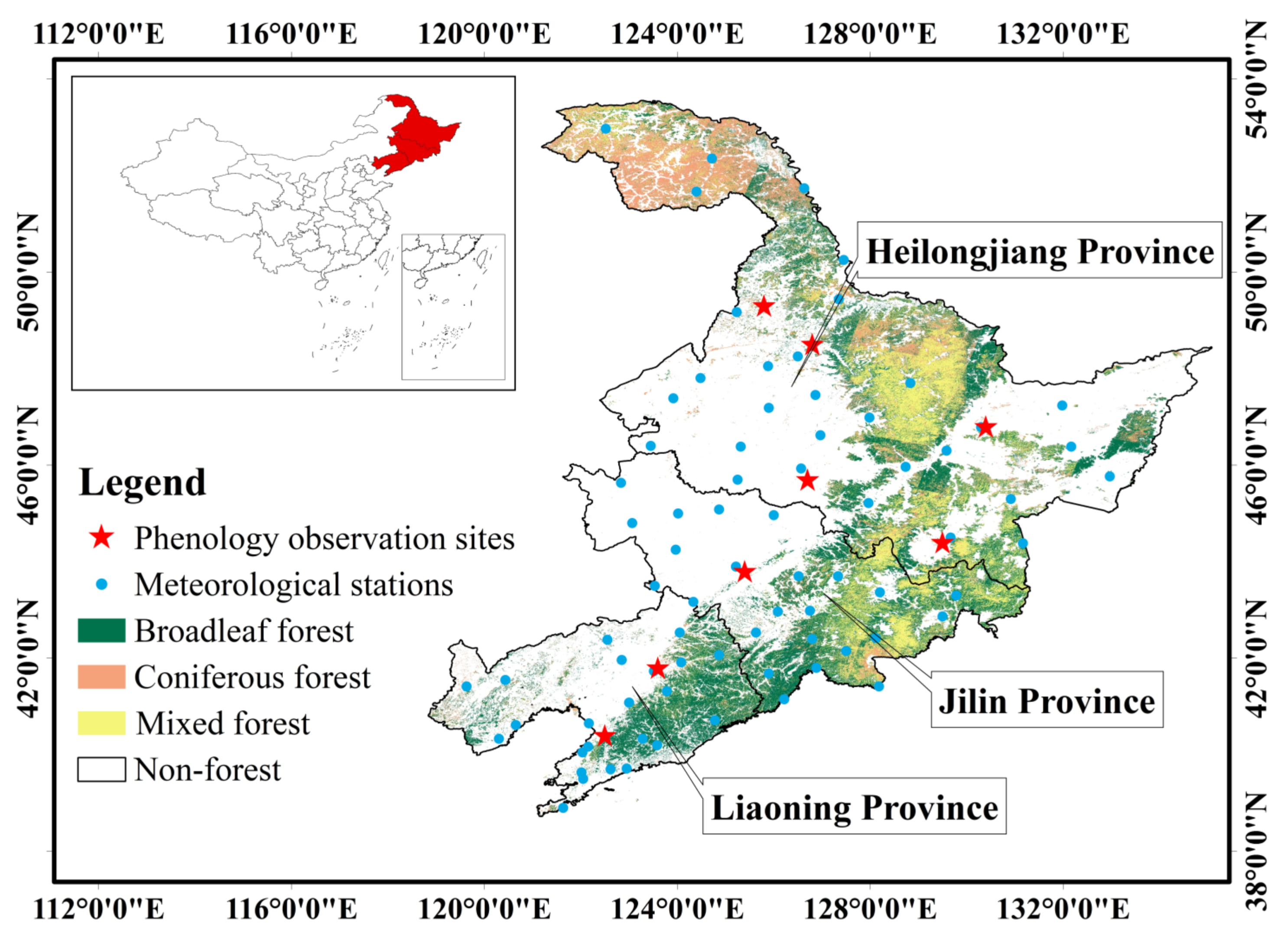
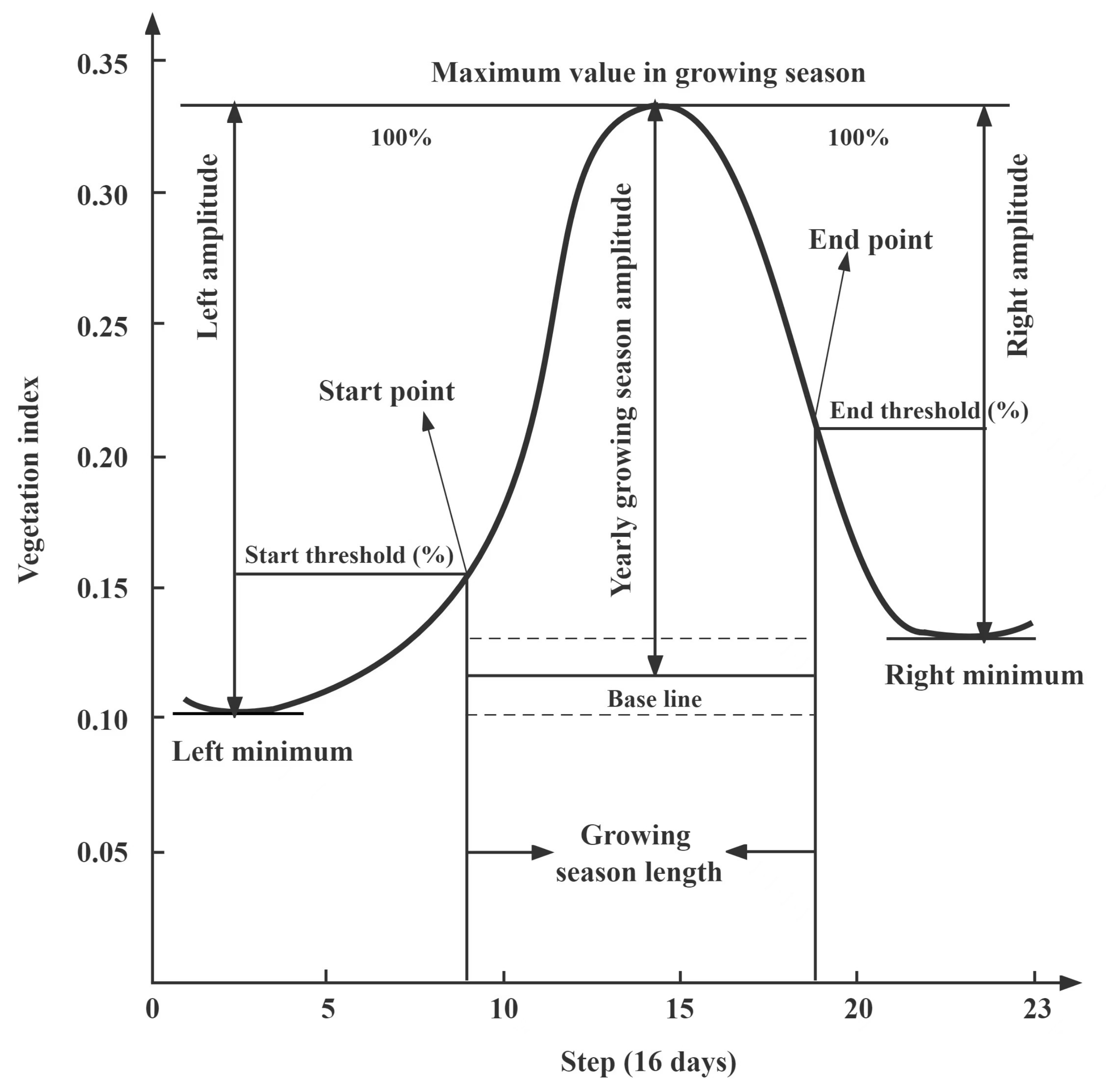
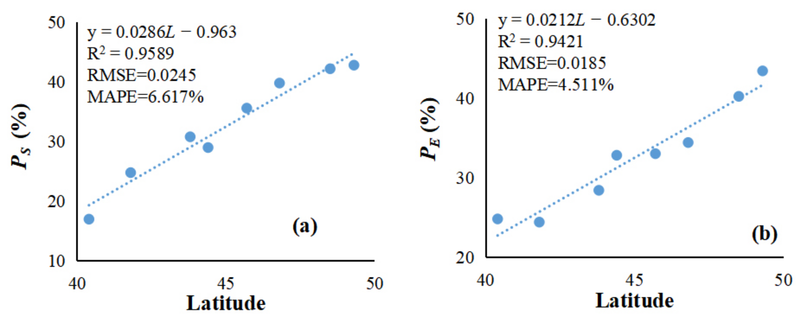
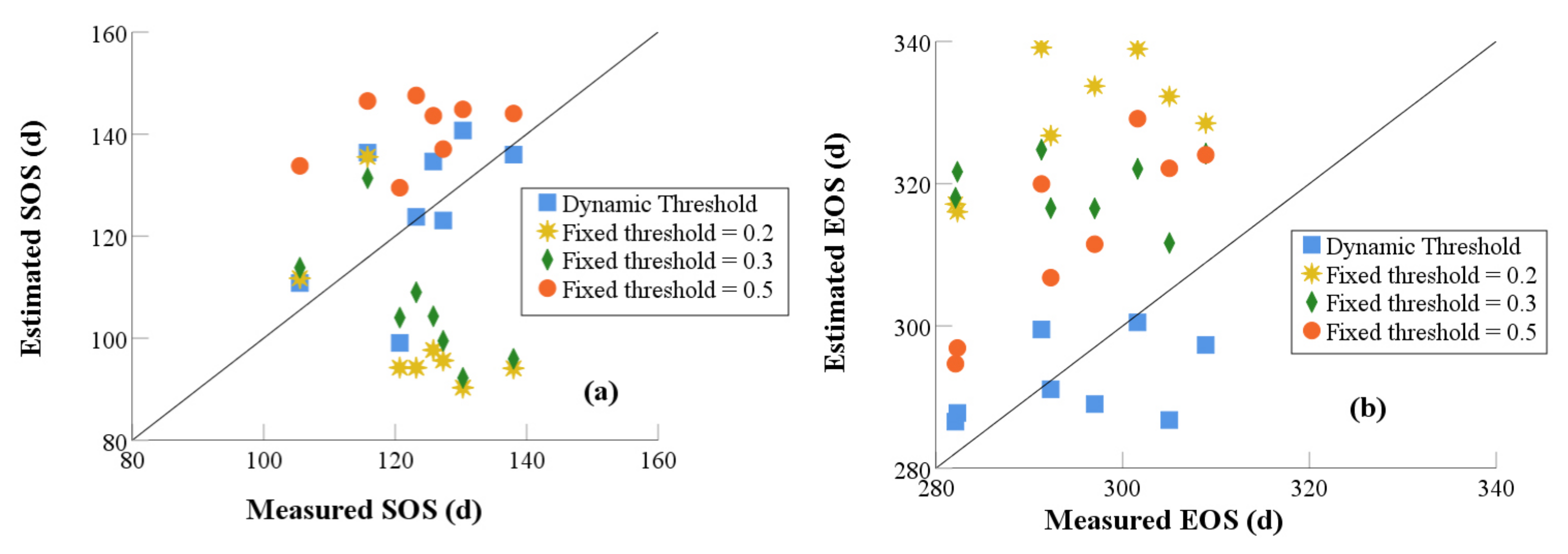
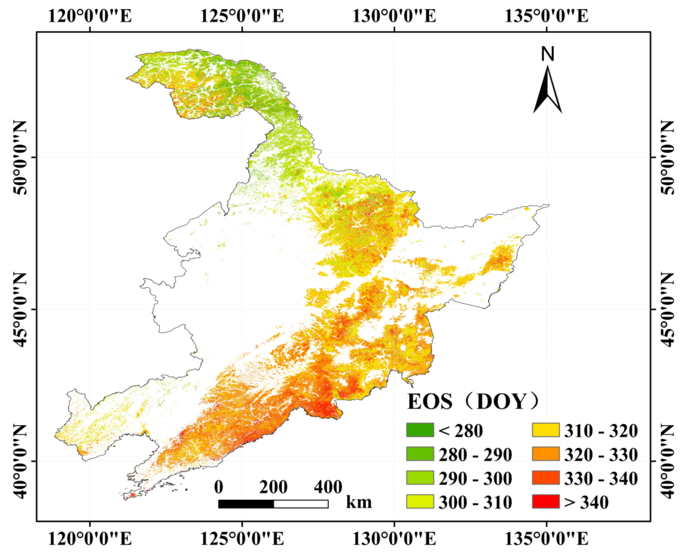
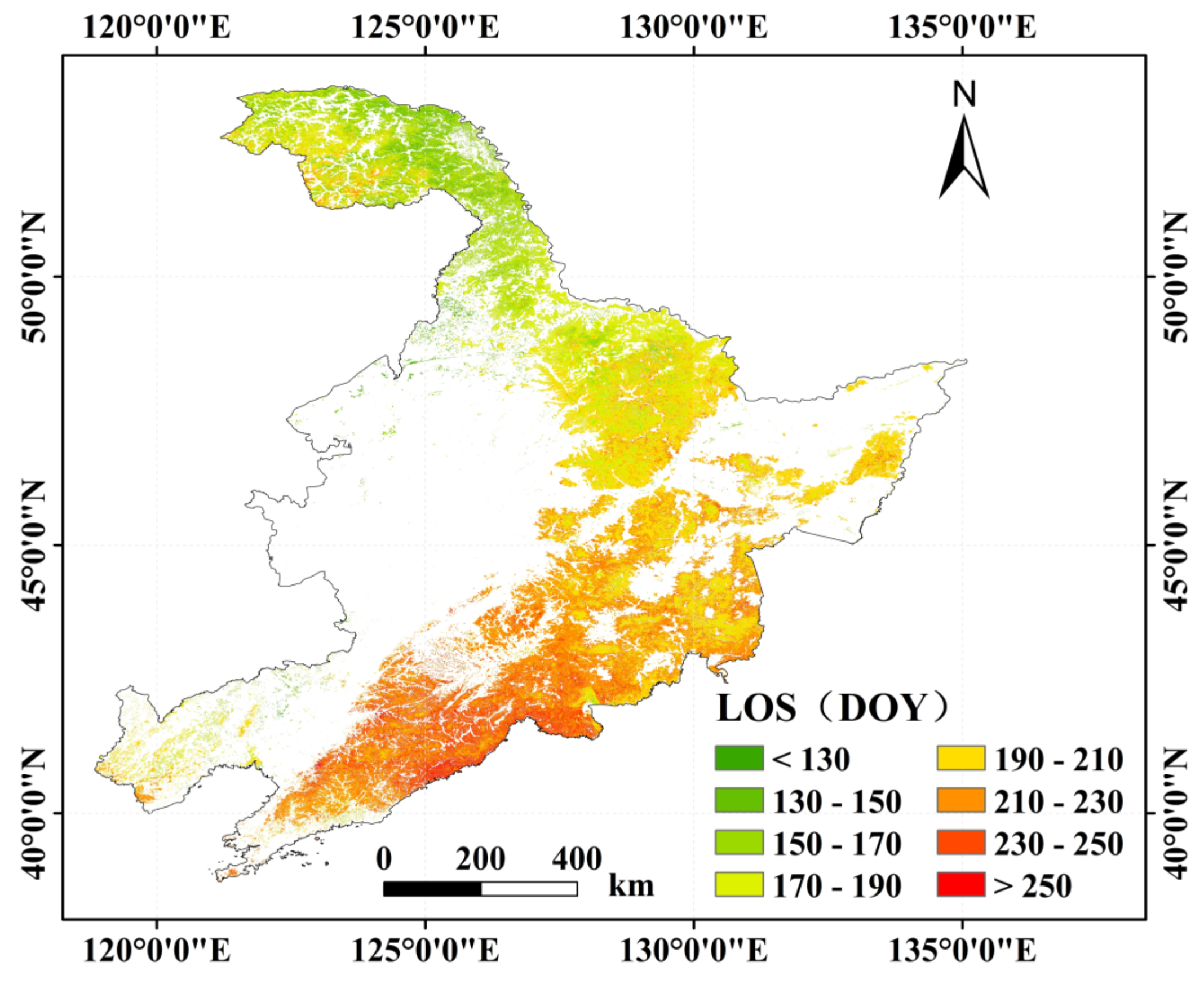
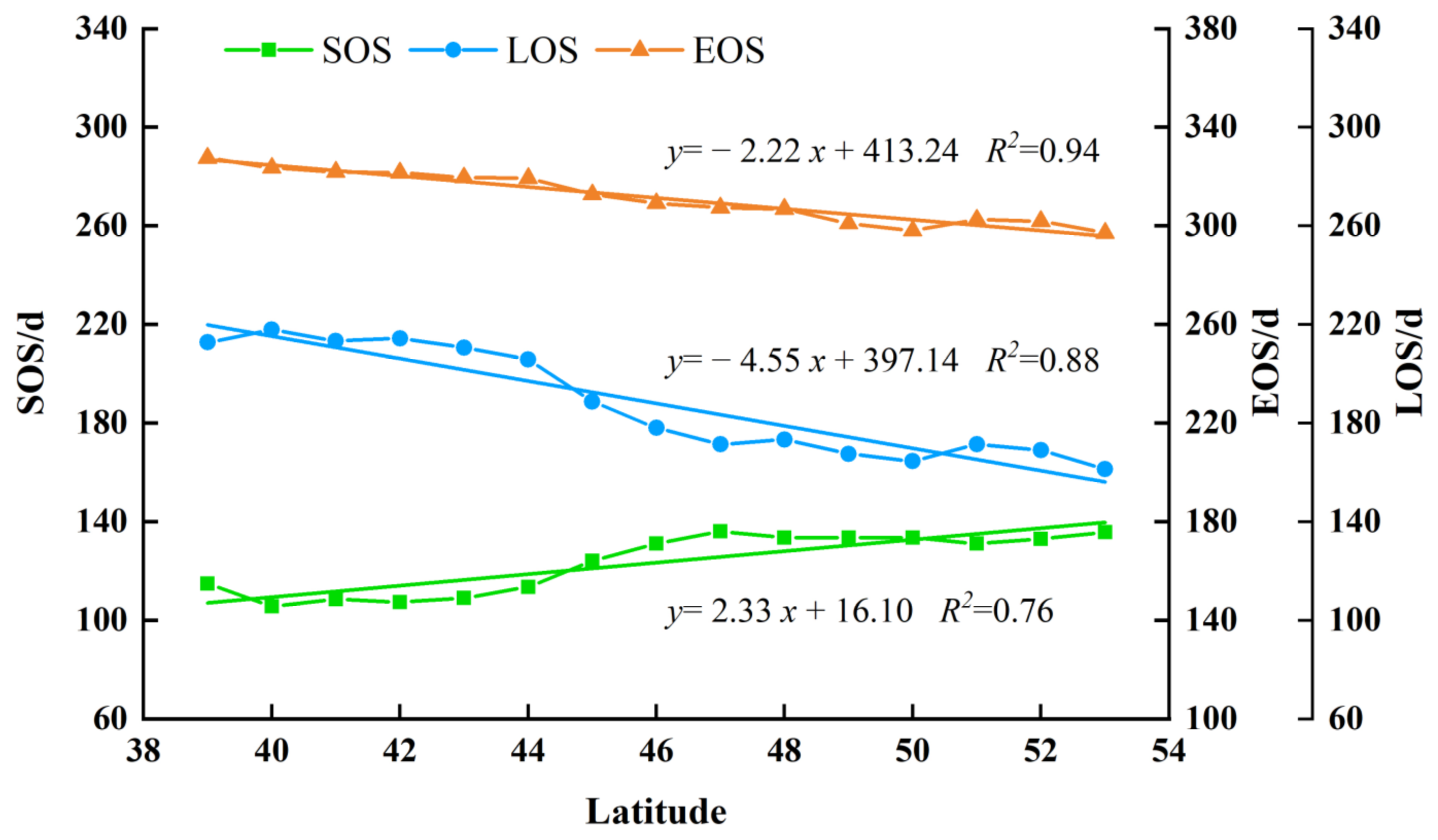
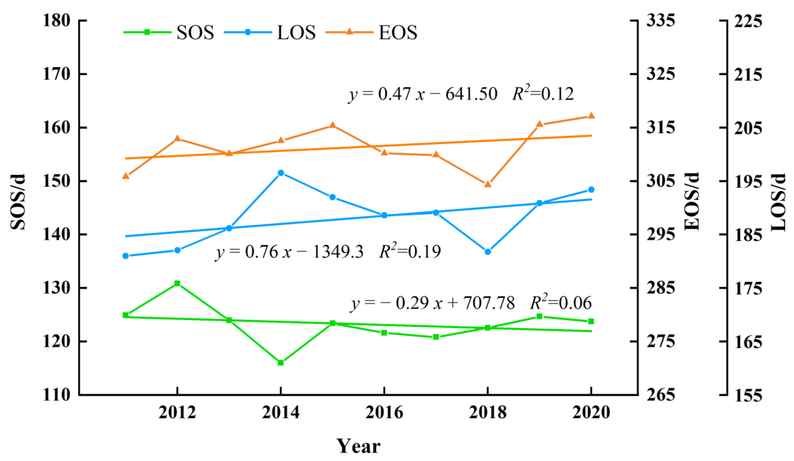
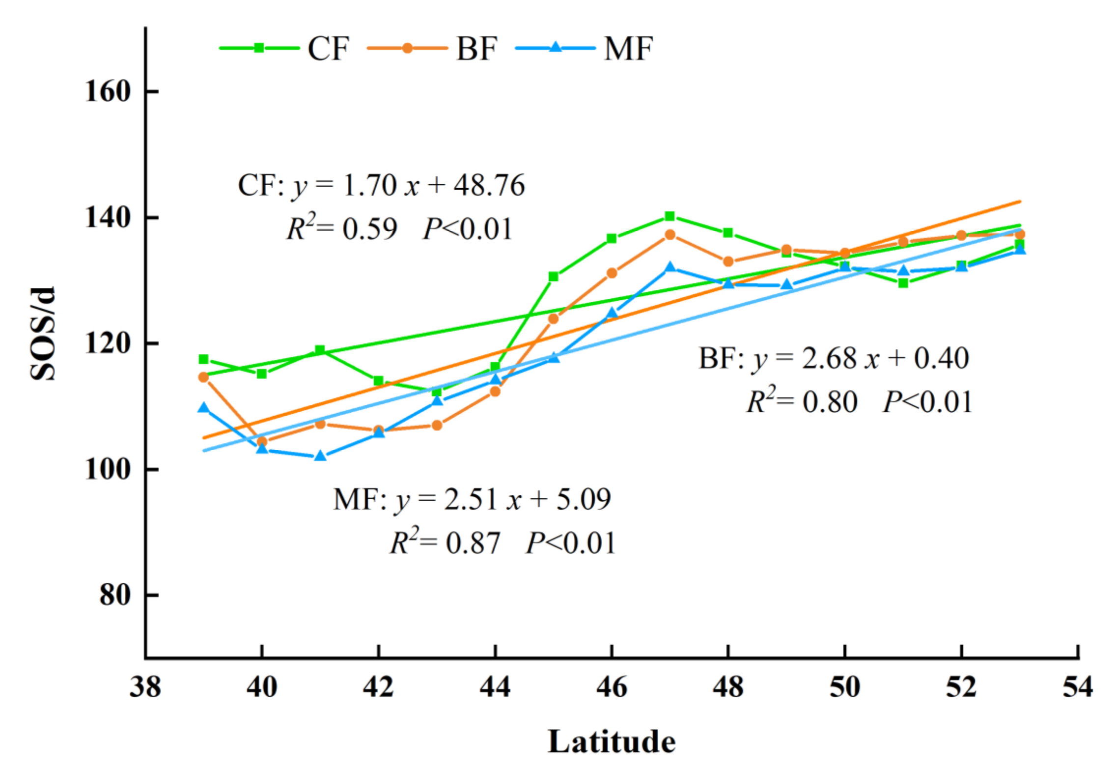
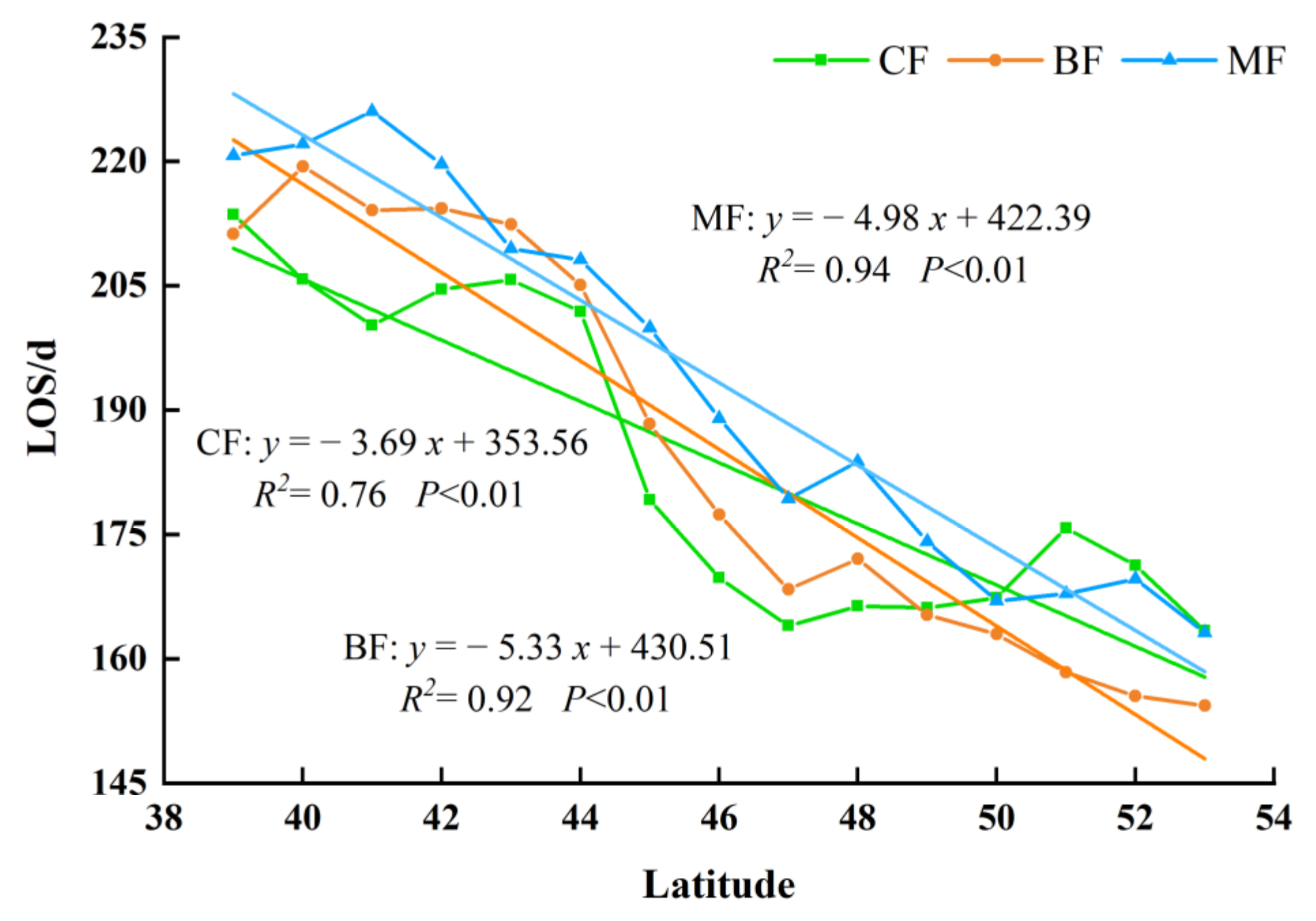
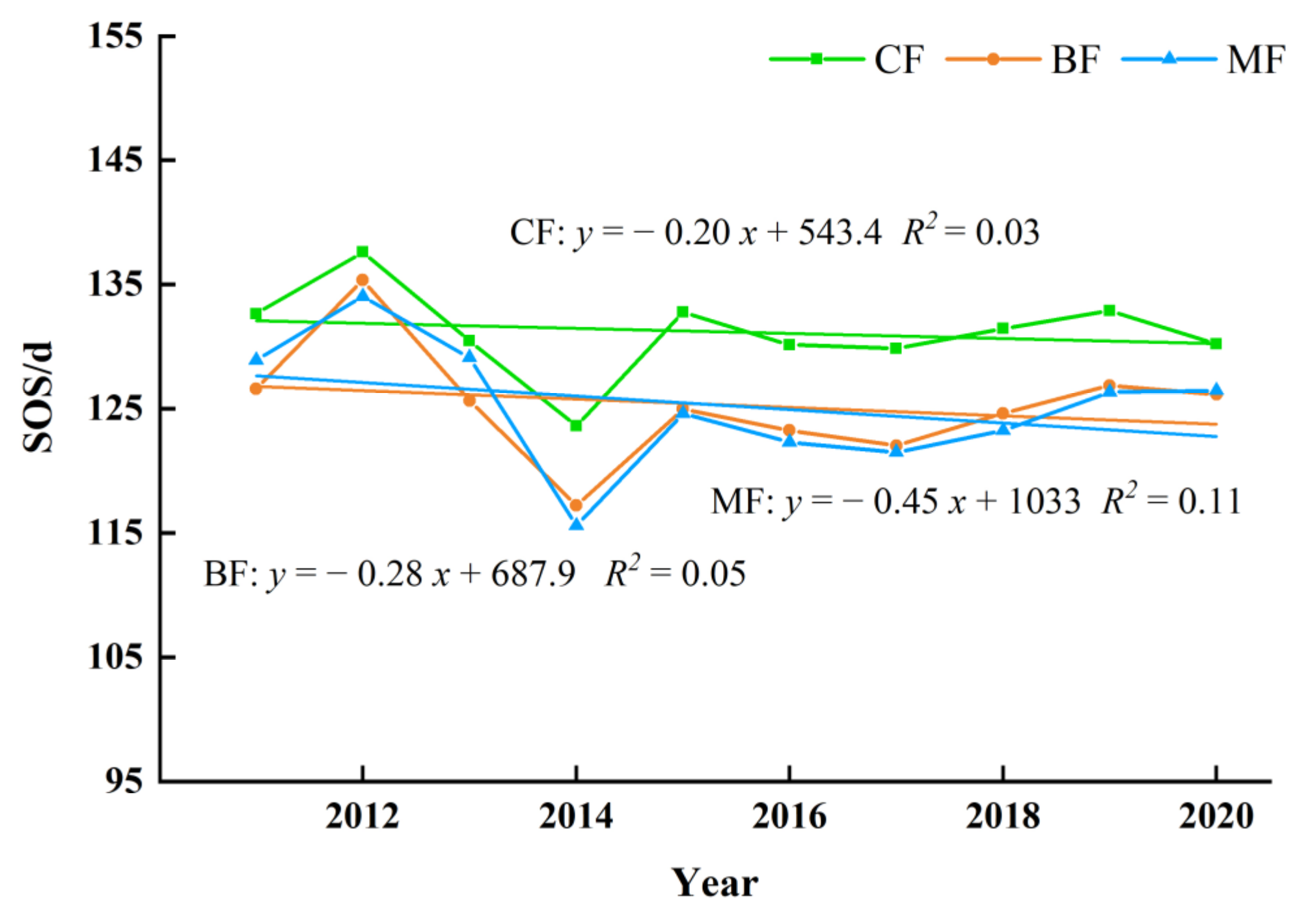
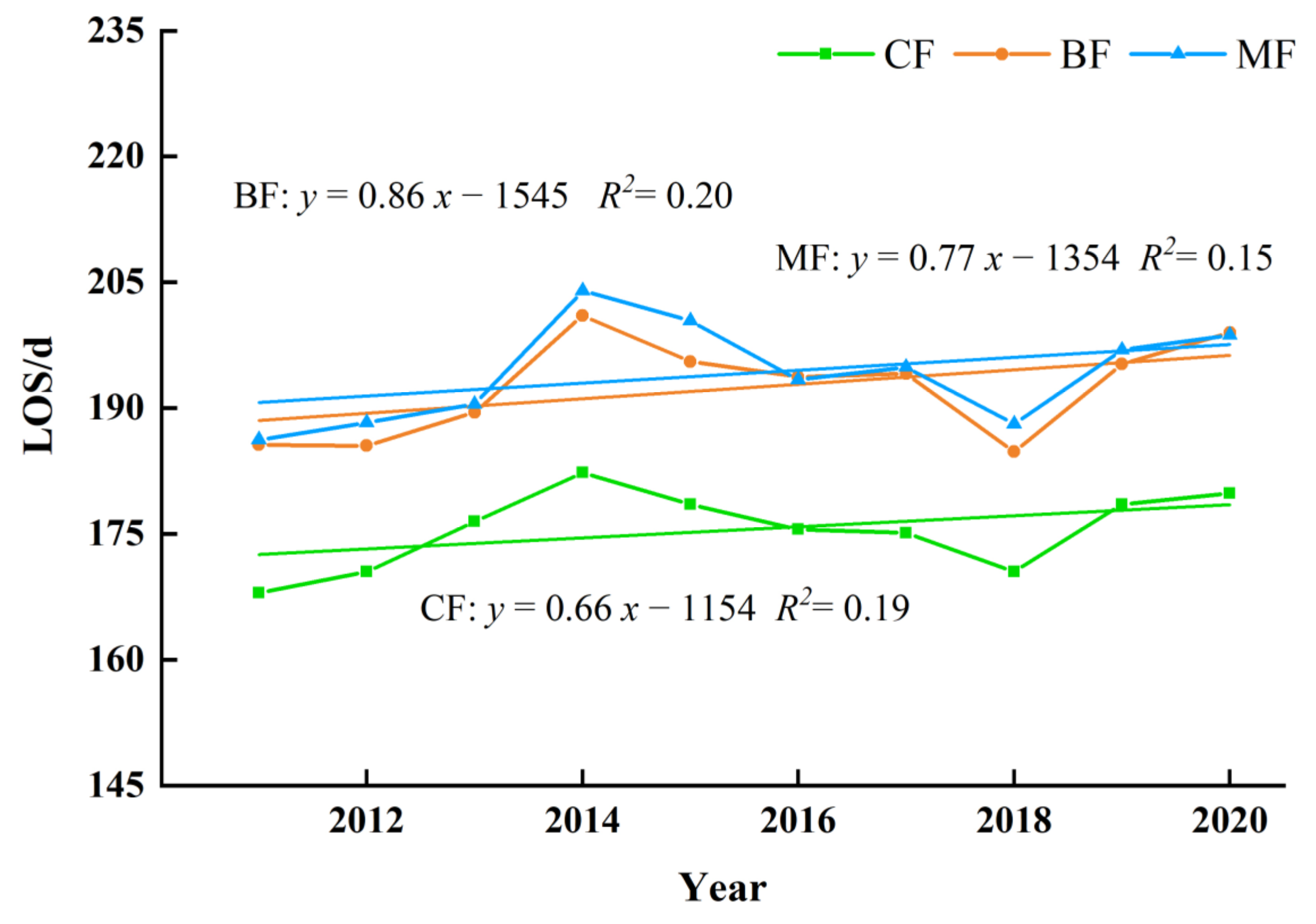
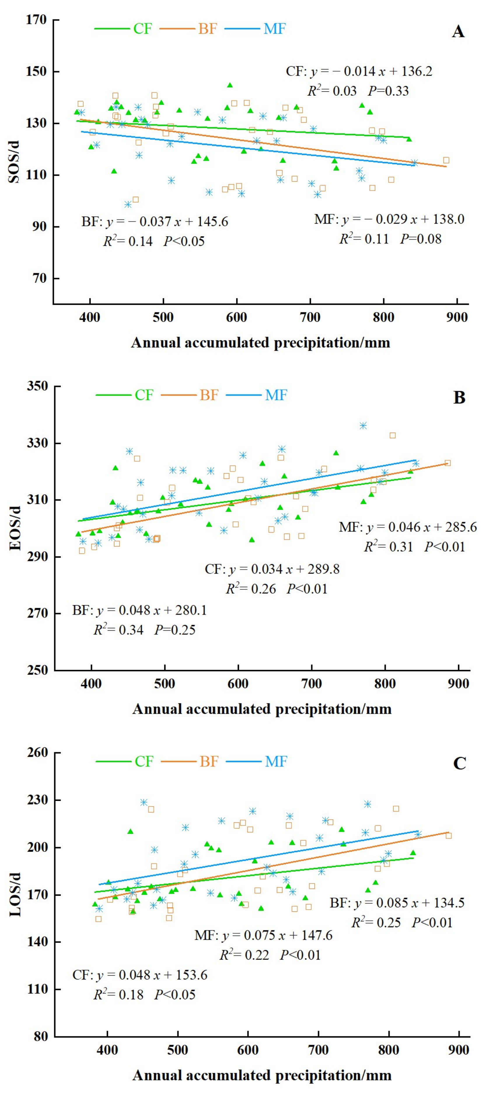
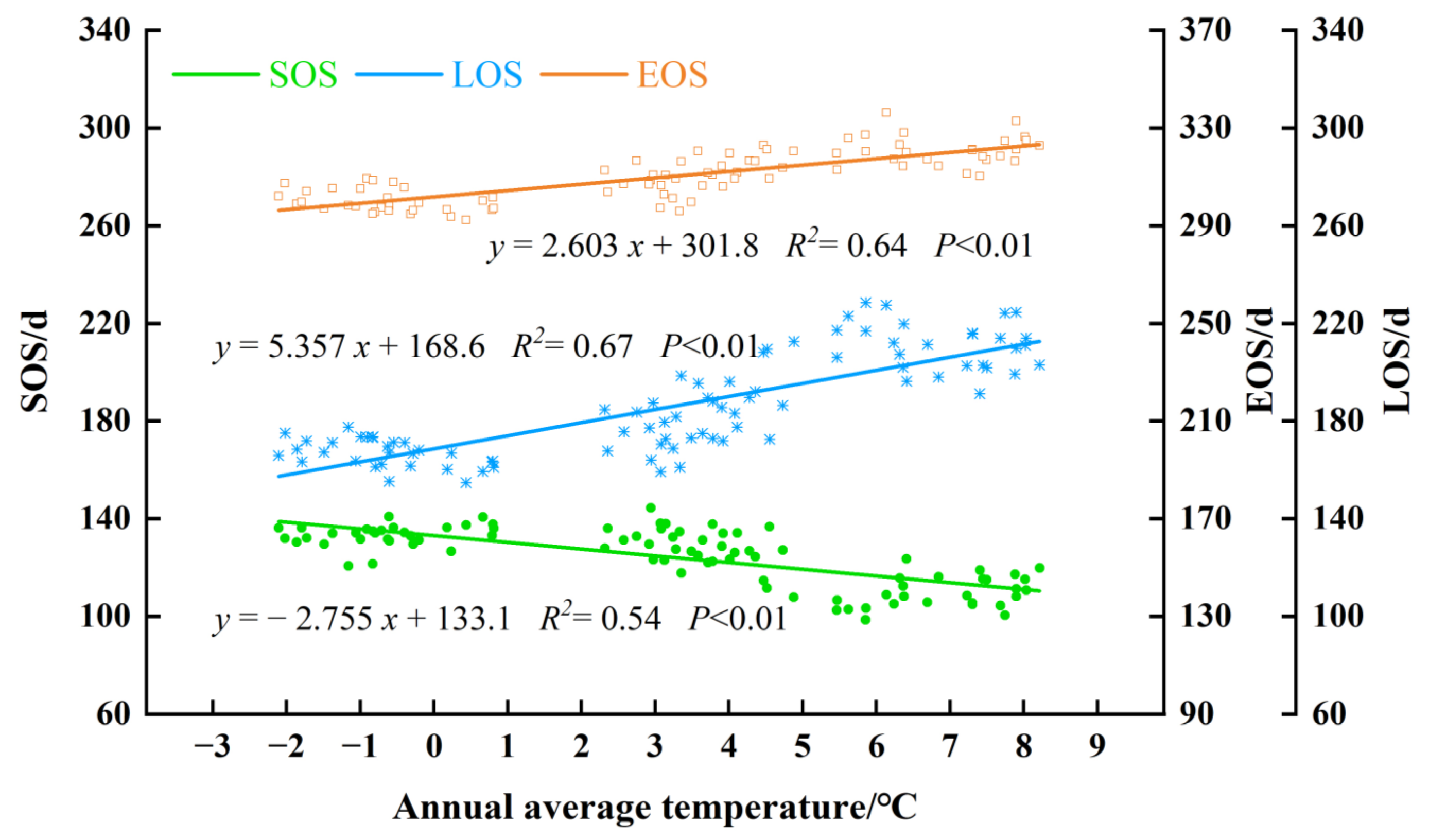
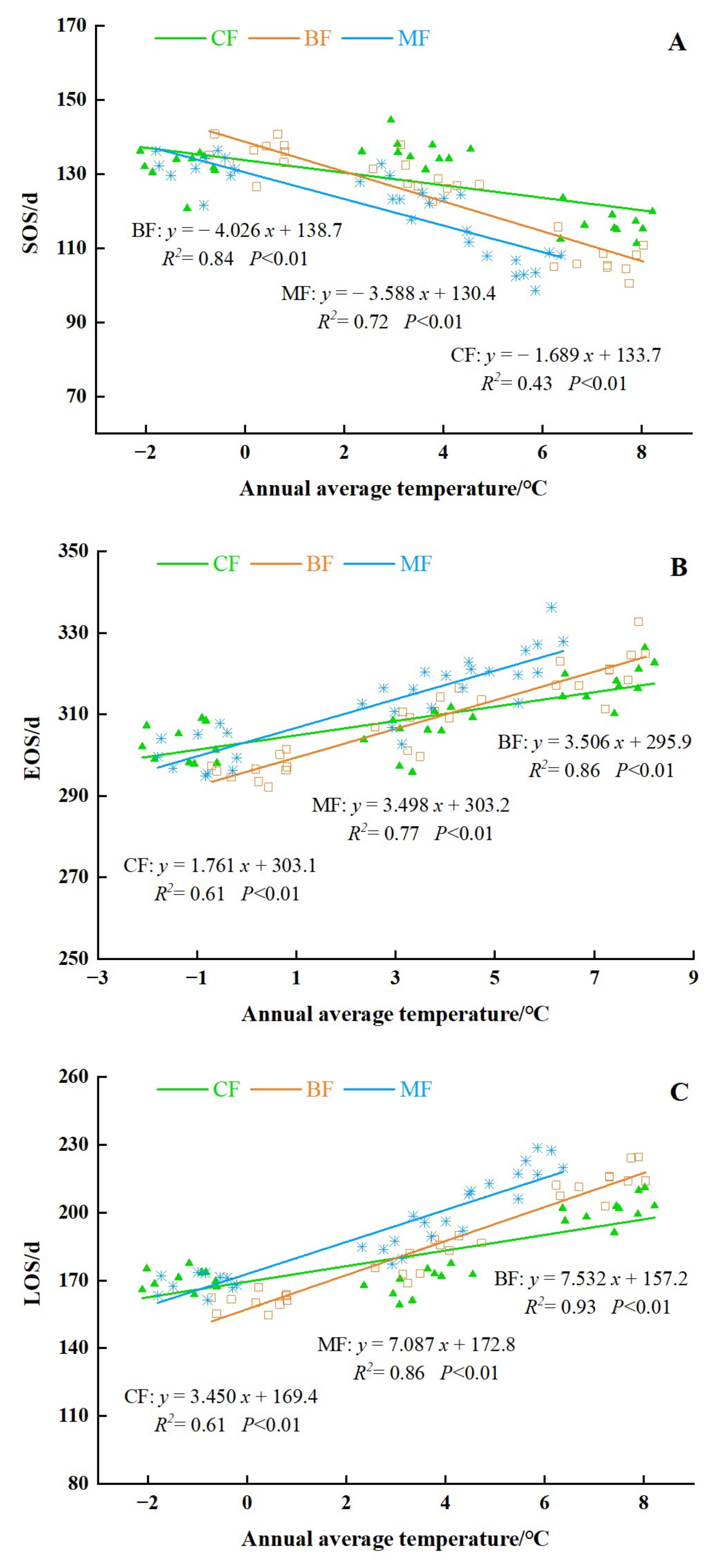
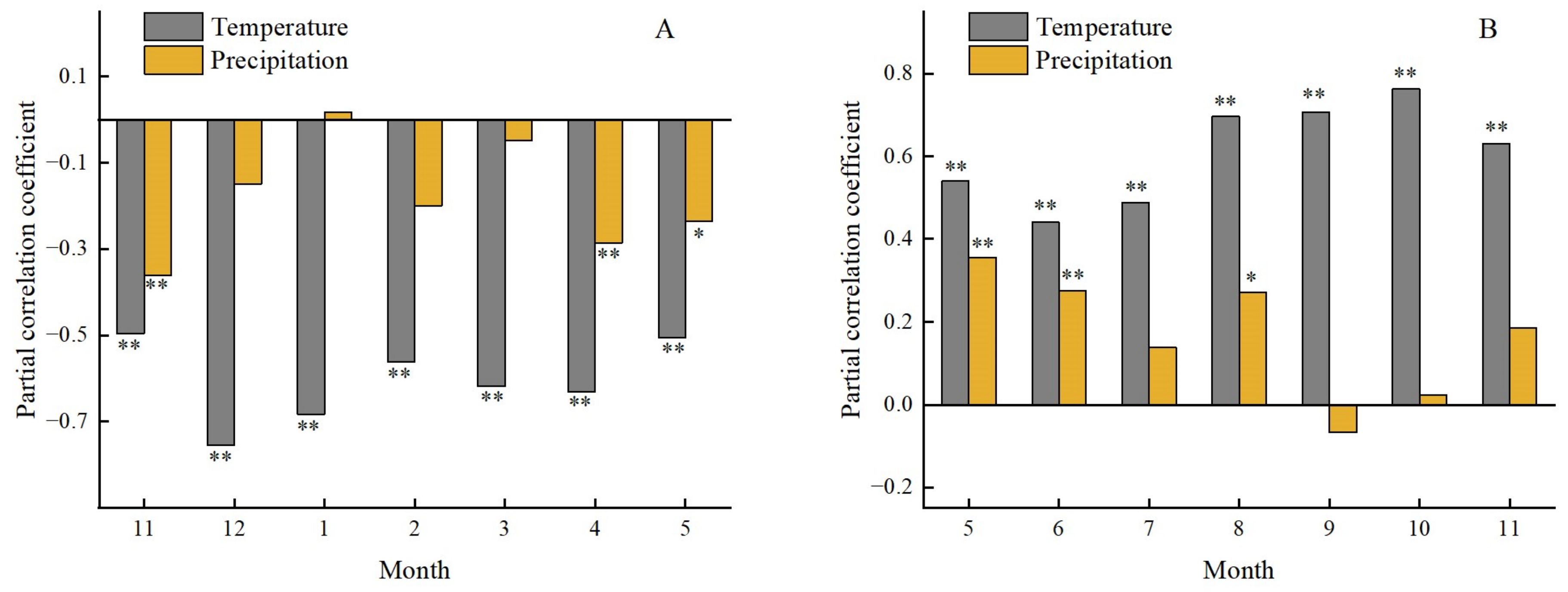
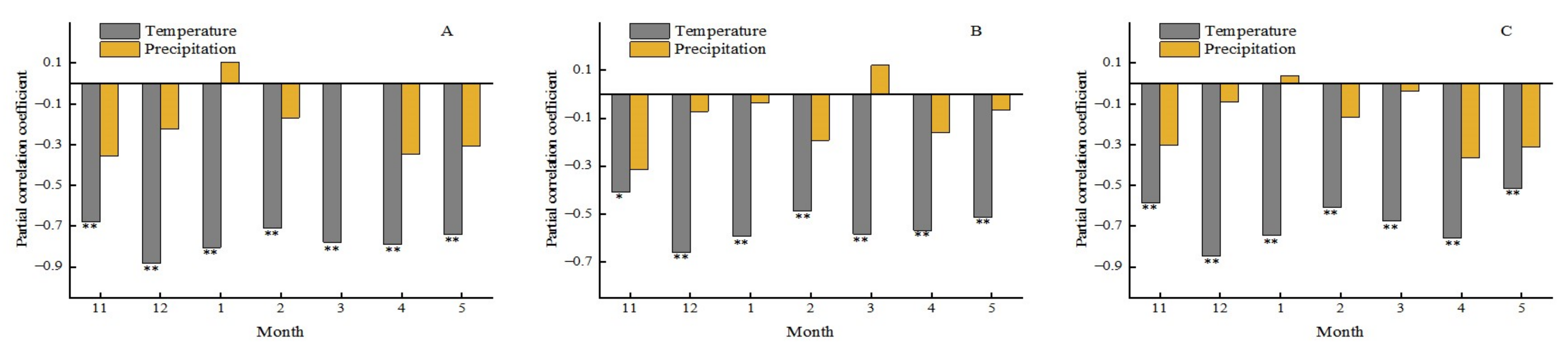
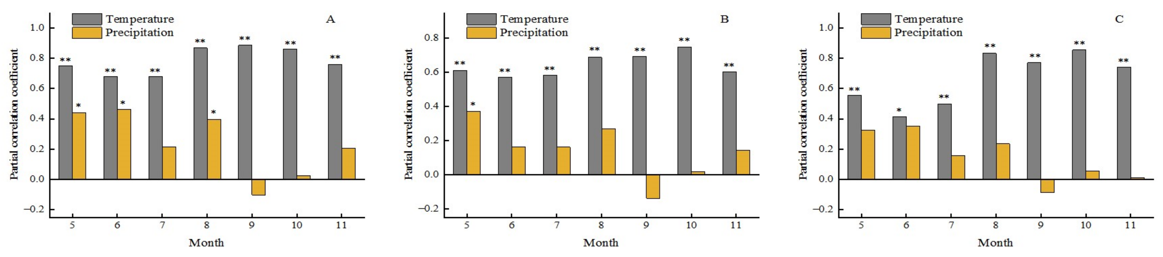
Table 1.
The statistical information of meteorological stations in the research area from 2011 to 2020.
Table 1.
The statistical information of meteorological stations in the research area from 2011 to 2020.
| Max | Min | Mean | |
|---|---|---|---|
| annual average temperature (°C) | 12.9 | −4.11 | 5.19 |
| annual cumulative precipitation (mm) | 1499.4 | 192.5 | 586.8 |
Table 2.
The mean forest phenological parameters of each station over the years.
| Station Name | Latitude | Longitude | Mean SOS/DOY | Mean EOS/DOY |
|---|---|---|---|---|
| Gaizhou | 40.4 | 122.5 | 105.5 | 308.9 |
| Shenyang | 41.8 | 123.6 | 115.8 | 305 |
| Changchun | 43.8 | 125.4 | 120.7 | 301.6 |
| Mudanjiang | 44.4 | 129.5 | 123.2 | 297 |
| Harbin | 45.7 | 126.7 | 127.3 | 291.3 |
| Jiamusi | 46.8 | 130.4 | 125.8 | 292.3 |
| Dedu | 48.5 | 126.8 | 138 | 282.3 |
| Nengjiang | 49.3 | 125.8 | 130.3 | 282.1 |
Table 3.
Detailed descriptions of research data.
| Type | Variables | Dataset | Resolution | Source |
|---|---|---|---|---|
| Vegetation Index | NDVI | MODIS NDVI | 250 m | NASA |
| Meteorological Data | Temperature, Precipitation | - | - | NOAA |
| Land Cover Type | Coniferous forest (CF), Broadleaf forest (BF), Mixed forest (MF). | FROM-GLC | 30 m | Pro. Peng Gong at Tsinghua University |
| Phenology Observation Data | Nenjiang, Dedu, Jiamusi, Harbin, Mudanjiang, Changchun, Shenyang, Gaizhou | - | - | Chinese Phenological Observation Network |
Table 4.
The accuracy comparation of the extracted phenology.
| SOS | EOS | |||
|---|---|---|---|---|
| RMSE (d) | MAPE (%) | RMSE (d) | MAPE (%) | |
| Dynamic threshold | 11.875 | 7.623 | 9.012 | 2.440 |
| Fixed threshold = 20% | 30.182 | 22.269 | 34.846 | 11.577 |
| Fixed threshold = 50% | 19.607 | 14.723 | 19.015 | 6.118 |
Publisher’s Note: MDPI stays neutral with regard to jurisdictional claims in published maps and institutional affiliations. |
© 2022 by the authors. Licensee MDPI, Basel, Switzerland. This article is an open access article distributed under the terms and conditions of the Creative Commons Attribution (CC BY) license (https://creativecommons.org/licenses/by/4.0/).
Share and Cite
MDPI and ACS Style
Zheng, W.; Liu, Y.; Yang, X.; Fan, W. Spatiotemporal Variations of Forest Vegetation Phenology and Its Response to Climate Change in Northeast China. Remote Sens. 2022, 14, 2909. https://doi.org/10.3390/rs14122909
AMA Style
Zheng W, Liu Y, Yang X, Fan W. Spatiotemporal Variations of Forest Vegetation Phenology and Its Response to Climate Change in Northeast China. Remote Sensing. 2022; 14(12):2909. https://doi.org/10.3390/rs14122909
Chicago/Turabian StyleZheng, Wenrui, Yuqi Liu, Xiguang Yang, and Wenyi Fan. 2022. "Spatiotemporal Variations of Forest Vegetation Phenology and Its Response to Climate Change in Northeast China" Remote Sensing 14, no. 12: 2909. https://doi.org/10.3390/rs14122909
Note that from the first issue of 2016, this journal uses article numbers instead of page numbers. See further details here.