Initial Cross-Calibration of Landsat 8 and Landsat 9 Using the Simultaneous Underfly Event

Abstract

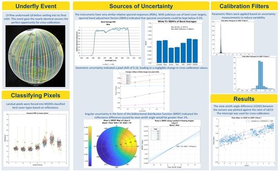
With the launch of Landsat 9 in September 2021, an optimal opportunity for in-flight cross-calibration occurred when Landsat 9 flew underneath Landsat 8 while being moved into its final orbit. Since the two instruments host nearly identical imaging systems, the underfly event offered ideal cross-calibration conditions. The purpose of this work was to use the underfly imagery collected by the instruments to estimate cross-calibration parameters for Landsat 9 for a calibration update scheduled at the end of the on-orbit initial verification (OIV) period. Three types of uncertainty were considered: geometric, spectral, and angular (bidirectional reflectance distribution function—BRDF). Differences caused by geometric uncertainty were found to be negligible for this application. Spectral uncertainty was found to be minimal except for the green band when viewing vegetative targets. BRDF models derived from the MODIS BRDF product indicated substantial error could occur and required development of a mitigating methodology. With these three contributions of uncertainty properly addressed, it was estimated that the total cross-calibration uncertainty for underfly data could be kept under 1%. The data collected during the underfly were filtered to remove outliers based on uncertainty analysis. These data were used to calculate the TOA reflectance and radiance cross-calibration values for each spectral band by taking the ratio of Landsat 8 average pixel values to Landsat 9. Initial results of this approach indicated the cross-calibration may be as accurate as 0.5% in reflectance space and 1.0% in radiance space. The initial results developed in this study were used to refine the cross-calibration of Landsat 9 to Landsat 8 at the end of the OIV period.

1. Introduction

Continuing an unbroken chain of Earth remote sensing that began with the launch of Landsat 1 in 1972, Landsat 9 was launched on 27 September 2021, from Vandenburg Air Force Base. After an initial check-out period of 90 days, Landsat 9 is acquiring imagery daily along with its virtual twin, Landsat 8. The two satellites each image the Earth’s surface over 16-day periods that are 8 days out of phase with each other. As a result, the entire globe is imaged by Landsat every 8 days with nearly identical instruments in each—the Operational Land Imager (OLI) and the Thermal Infrared Scanner (TIRS).

During the initial on-orbit verification (OIV) period, an underfly maneuver was performed on 11–17 November where Landsat 9 crossed underneath Landsat 8 as it was moved into its final orbit. As a result, the two spacecrafts imaged the same point on the Earth’s surface at the same time and from nearly the same location. This maneuver provided an unparalleled opportunity for the cross-calibration of the two instruments. The initial cross-calibration data analysis and results are reported in this paper. Results from this analysis were central to the initial calibration of Landsat 9 at the end of the OIV period. Following this introduction, the methodology used to estimate uncertainties, collect underfly data, and analyze underfly data will be presented. This will be followed by the results that were generated from this initial analysis, and the final section will be a summary and conclusions.

1.1. Landsat 8 and 9 Characteristics

One of the key design criteria for Landsat 9 was that it should be as similar to Landsat 8 as possible with respect to radiometric, geometric, spectral, and spatial performance. The goal was that Earth observing data collected from these two instruments should be indistinguishable from one another [1]. Both Operational Land Imagers (OLI) have the same 30 m ground sample distance (GSD), the same attitude control system, the same onboard radiometric calibration system, the same telescope and focal plane design, and the same spectral filters. In fact, the spectral filters for the Landsat 9 OLI (or OLI-2) were chosen from the same lot from which the Landsat 8 OLI filters were chosen. For purposes of cross-calibration via an underfly event, the most limiting factor historically has been differences in spectral bandpasses. The most significant difference between OLI and OLI-2 for purposes of radiometric calibration is that all 14 bits are downloaded for each image pixel for OLI-2, while only 12 bits are downloaded for OLI. With respect to TIRS on Landsat 8 and TIRS-2 on Landsat 9, the most significant difference is the added baffling that was put in place on TIRS-2 to mitigate the well-known stray-light problem on TIRS. Additional details on all these features are contained in [2].

1.2. Cross-Calibration Based on Underfly Events

Underfly maneuvers have been used often throughout the Landsat program. The first successful use of an underfly event for cross-calibration was conducted for the Landsat 4 and 5 Thematic Mappers (TM), described by Metzler and Malila [3]. At that time, Landsat scenes were very large with respect to available computational resources. Thus, the analysis was limited to a single scene pair. The results indicated that relative gain differences between the sensors ranged from 2% to 14%. Even though data were extremely limited in this analysis, the effort showed the value of cross-calibration using underfly maneuvers, because the Landsat 4 and 5 thematic mappers were essentially clones of one another built simultaneously.

Landsat 7, launched in 1999, was also raised into orbit such that it flew under Landsat 5. As a result, the instruments imaged the same region of the Earth’s surface from June 1–4 of that year, described by Teillet et al. [4]. This effort focused on analysis of large homogeneous areas from three scenes—Railroad Valley, Nevada; Niobrara, Nebraska; and Washington, DC. A key difference between the Landsat 5 TM and the Landsat 7 Thematic Mapper Plus (ETM+) was in the spectral bandpasses. At the time Landsat 7 was built, improvement in spectral filter design, as well as better understanding of atmospheric effects, allowed the development of filters with refined spectral bandpasses. Unfortunately, these differences translate to differences in instrument response even when the two instruments were imaging the same surface at the same time through the same atmosphere. These differences are also a function of surface reflectance properties, so they cannot be predicted or modeled. Therefore, they introduce a greater uncertainty to the process. Fortunately, the Railroad Valley surface reflectance was measured at the time of overpass and spectral differences could be accounted for. Results of this analysis indicated good agreement in bands 1–3 (blue, green, red), but poor agreement at the longer wavelengths.

With the launch of Landsat 8 in February of 2013, another opportunity for an underfly event occurred between Landsat 7 and Landsat 8. On 29–30 March 2013, Landsat 8 flew underneath Landsat 7 on its path toward final orbital insertion. A new era of Landsat instrumentation began with Landsat 8, as the thematic mapper instruments were retired in favor of a pushbroom scanner design. Additionally, dramatic changes in spectral bandpasses were incorporated to remove the effects of atmospheric absorption features. Mishra et al. describes the effort to perform a cross-calibration of the ETM+ with the new operational land imager (OLI) onboard Landsat 8 [5]. Dealing with the significant spectral differences between the sensors, the coincident image analysis was limited to several Saharan scenes for which a large of amount of hyperspectral information was available through the Hyperion sensor from the Earth Observing 1 (EO-1) mission. Results of this analysis indicated that the two instruments agreed to within 2% of each other with an uncertainty in the estimates of approximately 4%.

With the launch of Landsat 9, yet another underfly event was scheduled. The opportunity this time, however, far exceeded what was possible previously. As the two instrument sets, OLI/OLI-2 and TIRS/TIRS-2, are essentially carbon copies of each other, the substantial limitation of spectral differences was greatly reduced. Additionally, with modern computer capabilities, all coincident scene collects could be analyzed. Thus, a more robust analysis with lower uncertainties was possible.

2. Sources of Uncertainty

The great advantage of an underfly maneuver is that the signal paths for the energy received by the sensors are nearly identical and, when the two sensors are also nearly identical, uncertainties in the measurements are minimized. However, they do still exist. From a signal-path perspective, the two sources of uncertainty are the pointing errors that may occur, and the differences in viewing/illumination geometry. Instrument errors are primarily due to spectral differences between the sensors. Each of these sources of uncertainty will be considered briefly in this section, and the quantified effects will help drive the data acquisition in the methodology section and the data analysis in the results section.

2.1. Spectral Uncertainty

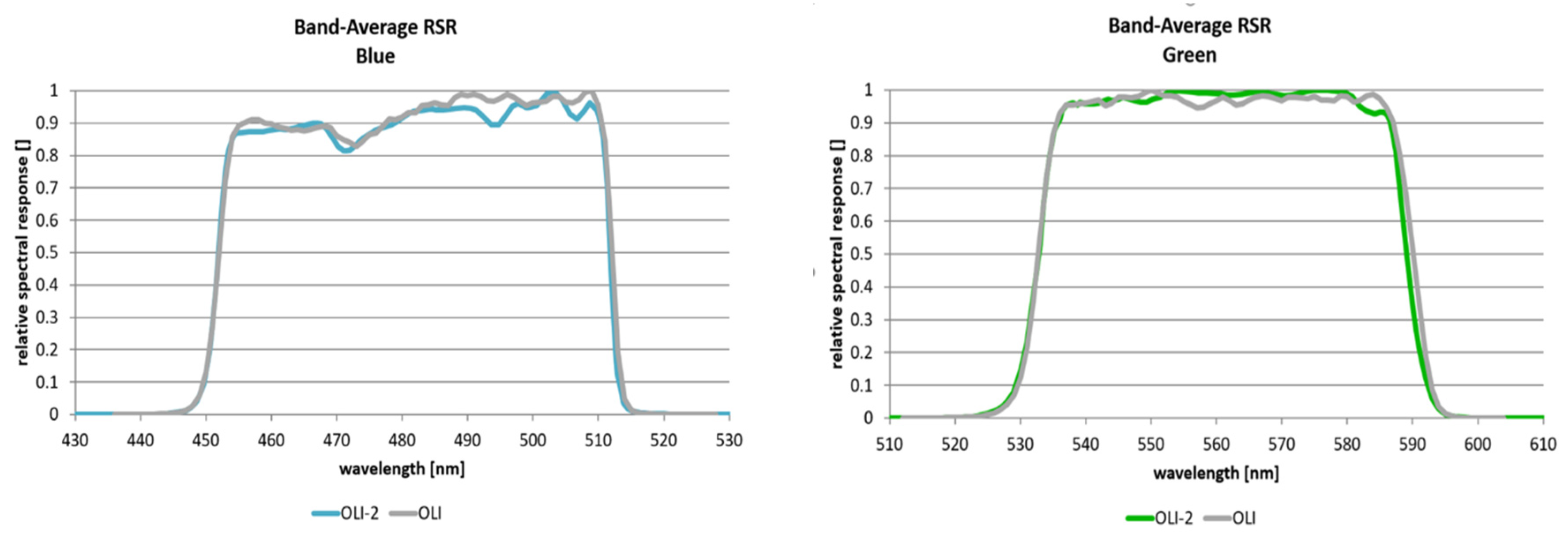
As the spectral filters for OLI and OLI-2 came from the original lot of filters developed for OLI, uncertainty from spectral differences was expected to be quite low. Figure 1 compares the spectral bandpasses, or relative spectral response (RSR) functions, for OLI and OLI-2 for several representative bands. It is clear that differences, though small, do exist.

To quantify differences that will occur in the sensor outputs due to spectral differences, the well-known spectral band adjustment factor (SBAF) was used. Details on the development and use of SBAF can be found in [6,7]. Basically, SBAF is the ratio of the reflectance level measured by two sensors that observe the same target simultaneously with the same illumination/viewing geometry, but with differing RSR functions. Any departure from an SBAF value of unity is a direct percentage measurement of the difference in output that would be expected from the sensors.

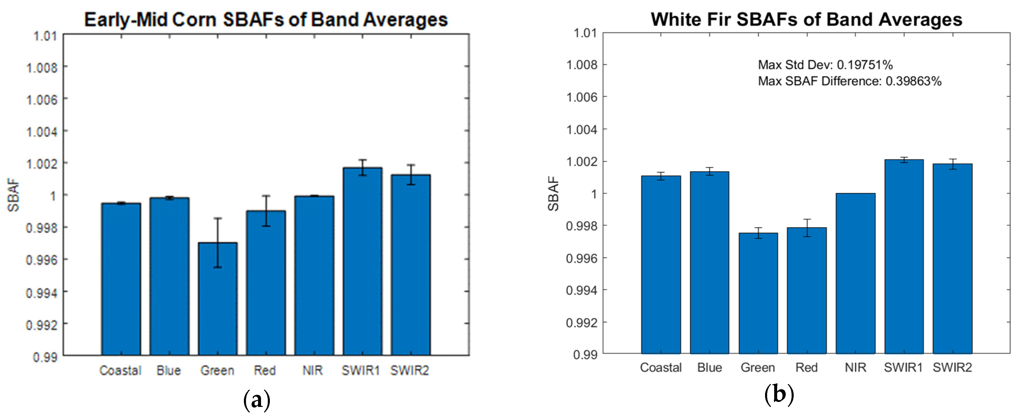
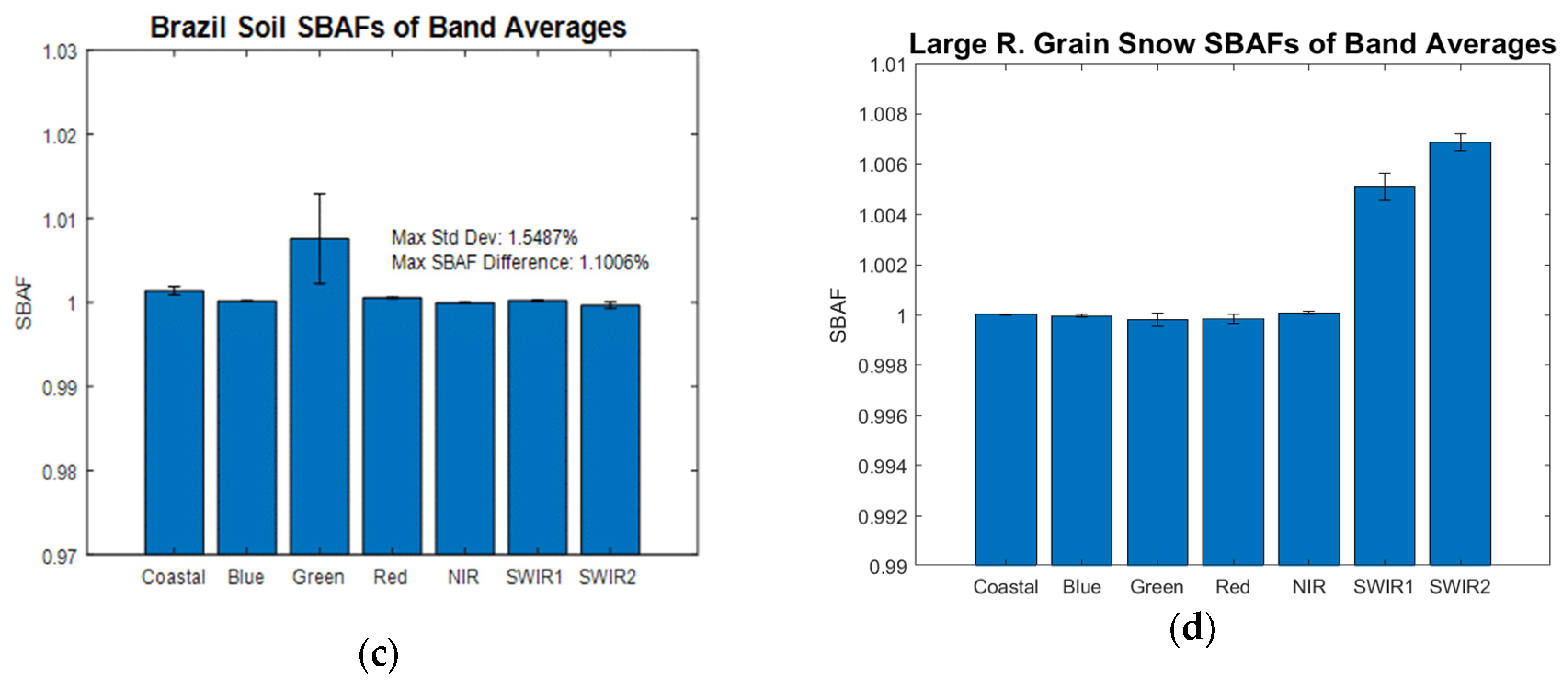
As SBAF is a function of target type, it was necessary to analyze a large variety of targets to understand the overall impact it would have. Examples of SBAF values for four major representative target types are shown in Figure 2. To obtain spectral information of targets, a variety of spectral databases were utilized: crop information came from the GHISA database [8], forest information from the ECOSTRESS library [9,10], soil information from the ICRAF-ISRIC Library [11], and snow information from the National Research Council of Italy Institute of Polar Sciences [12]. For all land cover types shown in Figure 2, the SBAF value uncertainties are all less than 1% (deviation from unity < 0.01). For vegetative cases, SBAF values tended to be less than 0.3% for all cases. For the case of soil targets, SBAF can, at worst, be on the order of about 0.7%, but only in the green band. While, for snow, SBAF is much larger than 0.5% in the SWIR. For the case of snow, the driver for the large uncertainty percentages is the low reflectivity of snow in the SWIR ranges. Thus, this can be easily avoided by not using snow-covered targets for cross-calibration of the SWIR bands. The TIRS instrument bands 10 and 11 also have slight differences in the RSRs; however, through multiple simulations with different target types, it was concluded that the SBAF in these bands would be at unity, to within 0.1%. Due to this, spectral uncertainty for TIRS was considered to be negligible for this experiment. In summary, it was felt that, with the judicious use of land cover targets, uncertainty due to spectral differences could be kept well below 0.5%.

2.2. Geometric Uncertainty

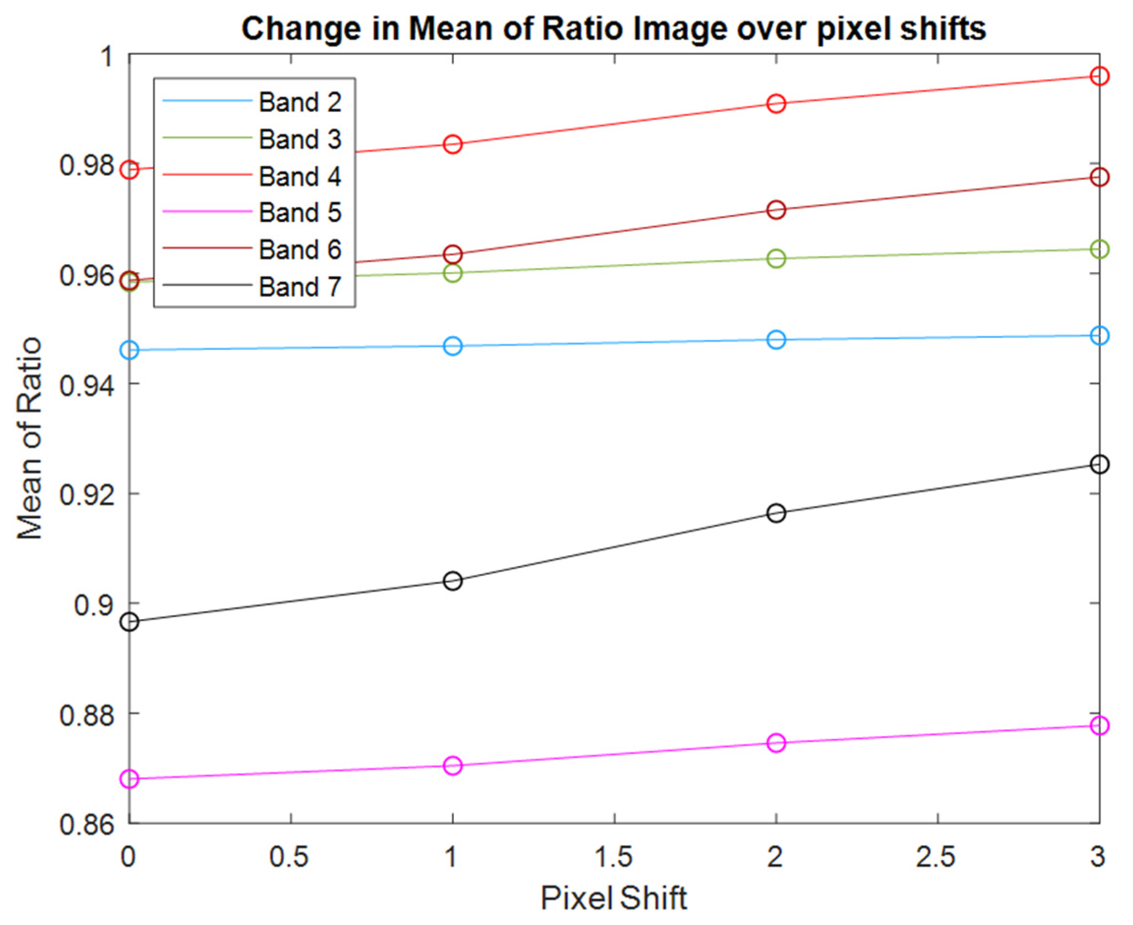
Pointing differences between the two sensors systems were analyzed to determine the degree of uncertainty that would occur for this situation. An analysis was performed using Landsat 7/8 underfly data using pixel shifts between the scene pairs to determine how much any error in pointing would change the cross-calibration ratio. Results from this analysis are shown in Figure 3. In this figure, pixel shift between the images is on the horizontal axis while the resulting ratio of reflectances between the two images is plotted along the vertical axis. As pixel shift increases from zero to three, a small change in the calibration ratio occurs; it is largest in band 7, ranging from approximately 0.895 to 0.925 or a change of about 3.3%. To understand how much shift might occur between Landsat 8 and Landsat 9 images, experts on Landsat geometry were consulted at USGS EROS (Choate, Michael. Interview. Conducted by Dennis Helder, 23 June 2021). Results of that discussion indicated that image-to-image errors would be on the order of 5 m. Since Landsat GSD is 30 m, this represents a pixel shift of 0.16. As can be seen from Figure 3, this leads to a very small change in cross-calibration ratio. Thus, uncertainties due to pointing errors were deemed to be negligible for this application.

Uncertainty due to differences in viewing/illumination geometry also need to be considered because, during the underfly maneuver, the two sensors have the exact same geometry for only an instant in time. During the course of the maneuver, the sun angle for any given target will be very similar for both sensors, but the viewing angles will change significantly. Worst case, at the beginning and end of the maneuver, when there is minimal image overlap, one sensor will be viewing 7.5° to the west while the other will be viewing 7.5° to the east. Thus, there will be a viewing zenith angle difference (VZAD) of 15°. Since the viewing azimuth angle for the sensors is nominally east/west or, more exactly, nominally 98° and 278° due to the 98° orbital inclination of Landsat, the sensors will be imaging close to the principle plane (that is, the situation where the sensor, target, and sun are contained in a plane) during imaging in the northern hemisphere, and close to the cross-principle plane (orthogonal to the principle plane) in the southern hemisphere, as the sensors complete imaging during the descending portion of the orbit. This geometry occurs because the underfly maneuver occurred on 11–17 November 2021.

2.3. Angular Uncertainty

Even slight differences in viewing and illumination angles when observing a target will result in the sensors capturing slightly different reflectances. Reflectance of surfaces as function of viewing/illumination angle is modeled by target-specific bidirectional reflectance distribution functions (BRDF). Thus, to understand the uncertainty due to viewing angle differences, it was necessary to use a BRDF modeling approach. The Ross–Li BRDF model as used by the MODIS sensors was chosen, since it is broadly accepted by the remote-sensing community and a large amount of data exists [13,14,15]. However, drawbacks of this approach include the fact that the Ross–Li model was developed primarily for vegetation and the spatial resolution of the MODIS sensors is much larger than Landsat’s.

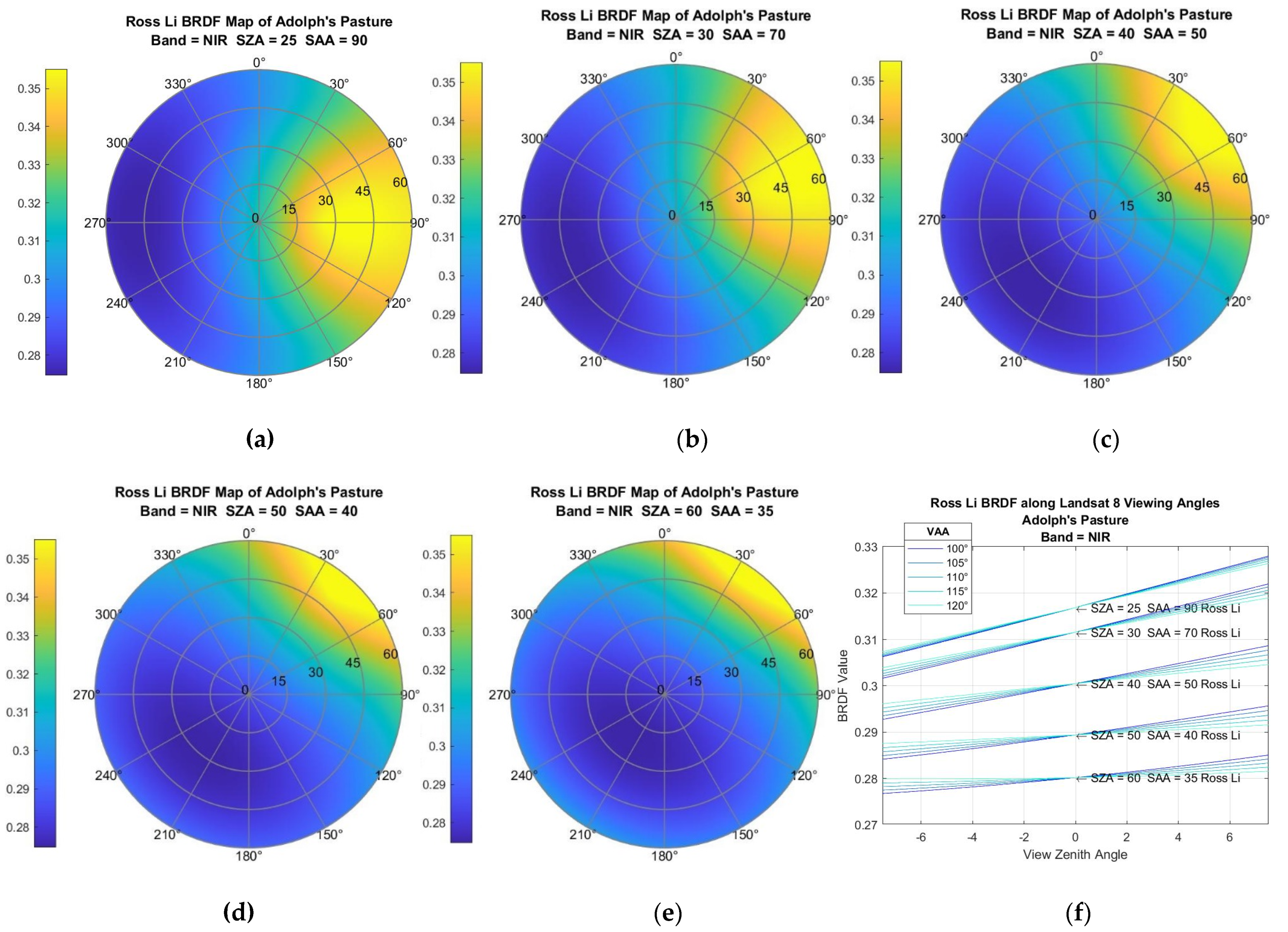
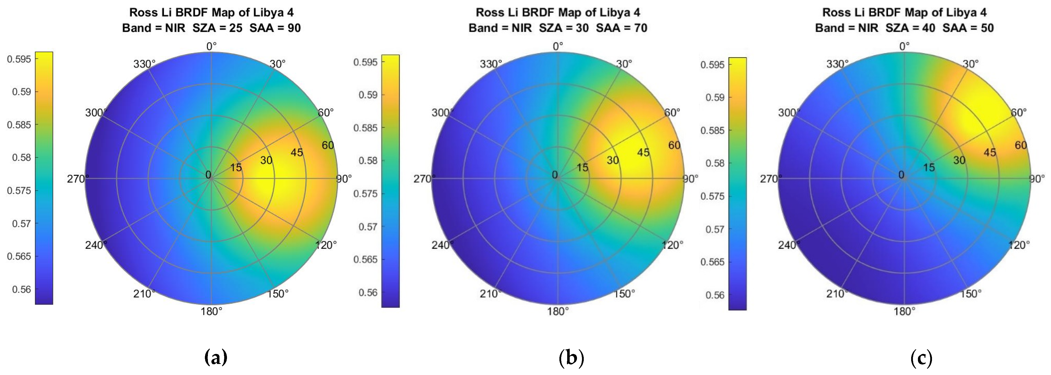
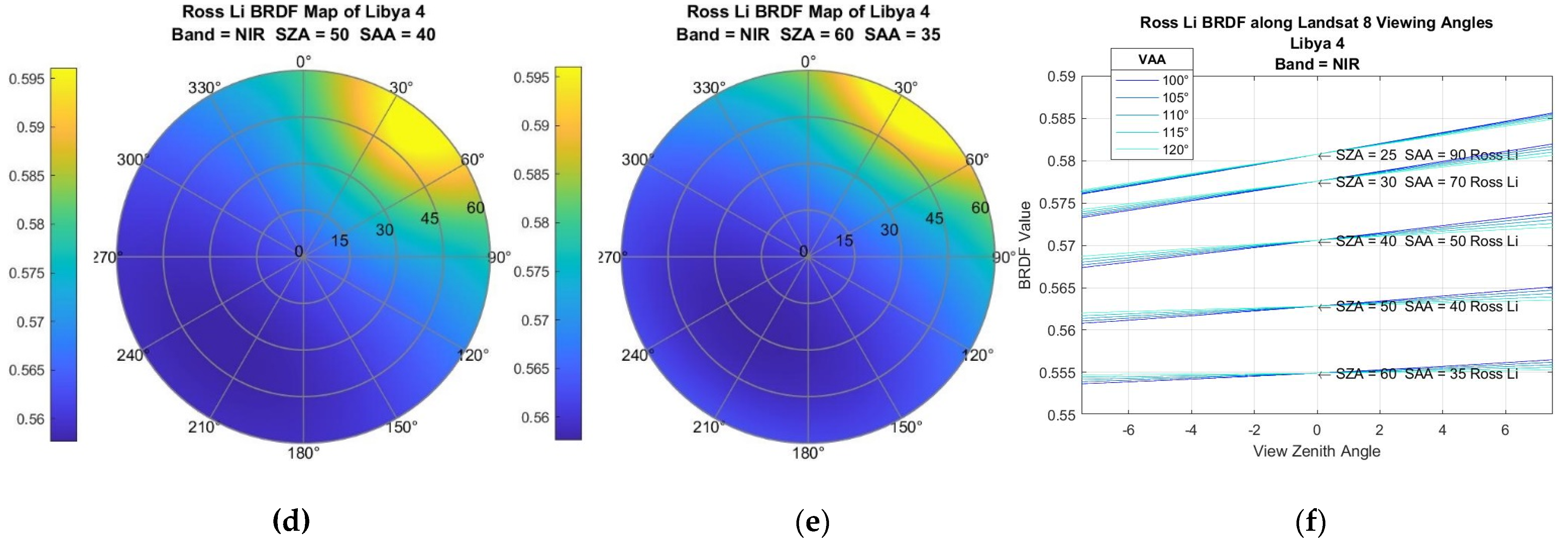
To understand the impact of BRDF on the uncertainty for the underfly maneuver, a simple analysis was performed on two land cover types—a grassy pasture in east central South Dakota (well known to one of the authors) and desert sand (from the well-known Libya 4 calibration site). Examples of the BRDF models obtained from MODIS observations (the MCD43A1 MODIS product) of these locations in summer of 2021 are shown in Figure 4 and Figure 5. From these figures, we see that the hot spot (the yellow region indicating higher reflectance) follows the location of the sun azimuthally and moves away from the origin as the SZA increases. Note that Landsat viewing angles are restricted to a region well within the 15° annular ring (±7.5°) and lie along a line roughly from 98° to 278°. If one extracts the data along this line and plots them as a function of VZA, the plot in the lower-right corner of the figure results. The key results to note here are that when VZA is restricted to the narrow range of Landsat angles, the curves are very linear. Secondly, as the VAA moves further from the principal plane, the slope of the lines decreases. Conversely, even for small VZA differences, the change in BRDF becomes large very quickly. Analysis of these VZA differences indicated that when the VZA difference reaches 7°, the change in BRDF value can reach 6% or more depending on SZA and relative azimuth angle. Clearly, BRDF uncertainty is unacceptably large for cross-calibration purposes! Similar results were obtained for the Libya 4 site, which is much more Lambertian in nature than a vegetative site. Figure 5 shows the same type of linear relationship (graph in lower right), and also less sensitivity—in this case, BRDF uncertainty only reached 1.5% at a VZA difference of 7°.

Since current radiometric calibration techniques yield uncertainties on the order of 3%, this simple analysis shows that BRDF will likely cause unacceptably large uncertainty over vegetative sites and only marginally acceptable uncertainty over more Lambertian sites such as sand and soil. However, since Landsat only has a very limited view angle range of zero to ±7.5°, the very non-linear nature of BRDF can effectively be linearized over this small range. This implies that a linear model fit to view angle differences versus cross-calibration gain ratio will produce an intercept value that has the potential to be highly accurate due to the acquisition of non-zero VZA differences. Furthermore, since the two sensors will only be in position for VZAD = 0 for a brief period of time (just a few minutes), by expanding the analysis to include coincident image pixels where VZAD ≠ 0, a much more diverse dataset can be obtained and analyzed. This is the approach that is taken in the following section.

In summary, uncertainty due to spectral differences can be kept quite small, 0.2% or less, by the judicial use of target type for a few spectral bands, and uncertainty due to pointing errors will be negligible. Thus, only uncertainty due to BRDF will be appreciable and can be mitigated by taking advantage of the small VZA for Landsat and using linear models to fit cross-calibration estimates as a function of VZA differences between the sensors. Combining these uncertainties, which are considered statistically independent, leads to an estimated uncertainty of 1% or less. The effects of uncertainty derived in this section were instrumental for developing filtering parameters that would ultimately determine the cross-calibration ratios for this experiment.

3. Data-Acquisition Methodology

3.1. Spectral Characterization of Land Cover Types

The previous uncertainty estimation analysis, particularly with respect to spectral and angular uncertainty, indicated that it would be necessary to know what type of land cover best described each pixel used in the underfly cross-calibration in order to group the pixels appropriately before estimating cross-calibration gain ratios. To begin this effort, once again the MODIS product suite was utilized. The MODIS Land Cover Type product (MCD12Q1) classifies all locations on the Earth’s surface using the International Geosphere-Biosphere Programme (IGBP) convention shown in

Table 1. IGBP land cover class types.

Name	Value	Description
Evergreen Needleleaf Forests	1	Dominated by evergreen conifer trees (canopy > 2 m). Tree cover >60%.
Evergreen Broadleaf Forests	2	Dominated by evergreen broadleaf and palmate trees (canopy > 2 m). Tree cover >60%.
Deciduous Needleleaf Forests	3	Dominated by deciduous needleleaf (larch) trees (canopy > 2 m). Tree cover >60%.
Deciduous Broadleaf Forests	4	Dominated by deciduous broadleaf trees (canopy > 2 m). Tree cover >60%.
Mixed Forests	5	Dominated by neither deciduous nor evergreen (40–60% of each) tree type (canopy > 2 m). Tree cover >60%.
Closed Shrublands	6	Dominated by woody perennials (1–2 m height) >60% cover.
Open Shrublands	7	Dominated by woody perennials (1–2 m height) 10–60% cover.
Woody Savannas	8	Tree cover 30–60% (canopy > 2 m).
Savannas	9	Tree cover 10–30% (canopy > 2 m).
Grasslands	10	Dominated by herbaceous annuals (<2 m).
Permanent Wetlands	11	Permanently inundated lands with 30–60% water cover and >10% vegetated cover.
Croplands	12	At least 60% of area is cultivated cropland.
Urban and Built-up Lands	13	At least 30% impervious surface area including building materials, asphalt, and vehicles.
Cropland/Natural Vegetation Mosaics	14	Mosaics of small-scale cultivation 40–60% with natural tree, shrub, or herbaceous vegetation.
Permanent Snow and Ice	15	At least 60% of area is covered by snow and ice for at least 10 months of the year.
Barren	16	At least 60% of area is non-vegetated barren (sand, rock, soil) areas with less than 10% vegetation.
Water Bodies	17	At least 60% of area is covered by permanent water bodies. Has not received a map label because of missing inputs.

below. The table lists cover types into 18 categories, 13 of which are vegetative in nature. Water Bodies category is not useful to this project due to its inherent low reflectance. Barren consists of sand, soil, and rock, and this category is of special interest since these surfaces can be more Lambertian in reflectance characteristics. Ultimately, the Barren category was divided into dark soil, light soil, and sand for the underfly data analysis to reduce uncertainty driven by multiple cover types in one classification.

To understand how land cover type would drive BRDF sensitivity, the 2020 MODIS Land Cover Product was used to categorize MODIS BRDF estimates from early November 2020 (the time of year for the underfly maneuver) into the IGBP categories listed in Table 1. High-quality BRDF estimates (quality assessment = 0 or 1) were extracted from large regions of North America, South America, Africa, Asia and Australia. BRDF model parameters from MODIS product MCD43A1 were classified through corresponding use of the MODIS Land Cover Product into the appropriate IGBP category as listed in Table 1. Essentially, the two products were used in tandem to determine the BRDF parameters of each IGBP type. Preliminary analysis of these models, over the small angular values for Landsat (±7.5° for VZA), indicated that each IGBP land cover type had statistically differing BRDF parameters. As a result, it was decided to use all IGBP land cover types distinctly rather than merge any together when forming cross-calibration estimates.

3.2. IGBP Cover-Type Spectra Matching

Using the MCD12Q1 product, data were collected from chosen locations in South America, Africa, Asia, and Australia at various latitudes. As stated, dates from November 2020 were utilized in an effort to resemble conditions at the time of the underfly and cover most of the possible cases for all the land cover types. However, these IGBP class types do not have a 1:1 corresponding product with the Landsat sensors; this was remedied by matching the spectral signatures of IGBP cover types to a robust cover-type system that was compatible with Landsat.

As previously stated, the MODIS product MCD43A1 generates BRDF parameters for all of its pixels using the Ross–Li model, which has three kernel-weighting parameters: isotropic, volumetric, and geometric. This product was cross-referenced with the land cover-type product MCD12Q1 to produce BRDF models of all the land cover types across the world to help determine the best and worst latitudes for cross-calibration during the underfly period. The isotropic parameter could also be used to derive the MODIS average banded reflectance of each IGBP land cover type at nadir, shown in

Table 2. Average banded reflected for each IGBP land cover type.

IGBP #	1	2	3	4	5	6	7	8	9	10	12	14	15	16
Blue	0.026	0.020	0.086	0.030	0.025	0.055	0.084	0.038	0.045	0.087	0.078	0.042	0.540	0.143
Green	0.048	0.048	0.102	0.062	0.054	0.092	0.131	0.070	0.082	0.133	0.121	0.079	0.578	0.221
Red	0.045	0.034	0.108	0.052	0.043	0.146	0.193	0.061	0.084	0.162	0.151	0.082	0.586	0.308
NIR	0.256	0.335	0.219	0.314	0.309	0.276	0.306	0.321	0.316	0.318	0.313	0.327	0.519	0.369
SWIR1	0.183	0.191	0.144	0.235	0.207	0.409	0.416	0.233	0.277	0.355	0.355	0.270	0.125	0.468
SWIR2	0.094	0.079	0.095	0.108	0.091	0.319	0.343	0.113	0.164	0.250	0.246	0.159	0.093	0.428

, which could then be used to match with another land-cover classifying system that was compatible with Landsat. MODIS does not have an equivalent coastal aerosol band, so that band could not be referenced for the Landsat cover-type system. IGBP types 11 and 13 were not used because permanent wetlands would have low reflectivity, and the urban land cover type would have low pixel densities in any given scene, meaning both types would therefore be poor targets for this type of calibration. The MODIS collected reflectance values for IGBP type 15 would also not be referenced, as the Level-1 quality assessment band (BQA) would be used to identify snow pixels during the underfly. This band categorizes cloud pixels, cloud shadows, snow, and other useful information, so spectral matching with the MODIS IGBP snow cover type was unnecessary.

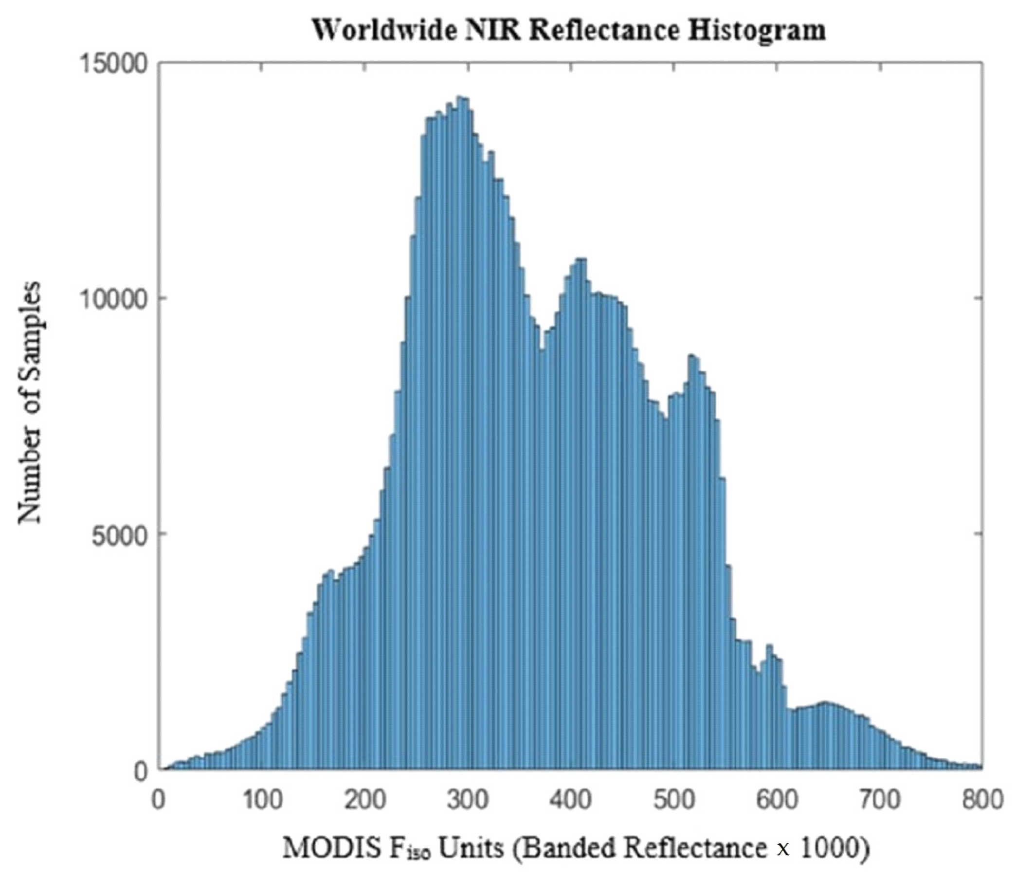
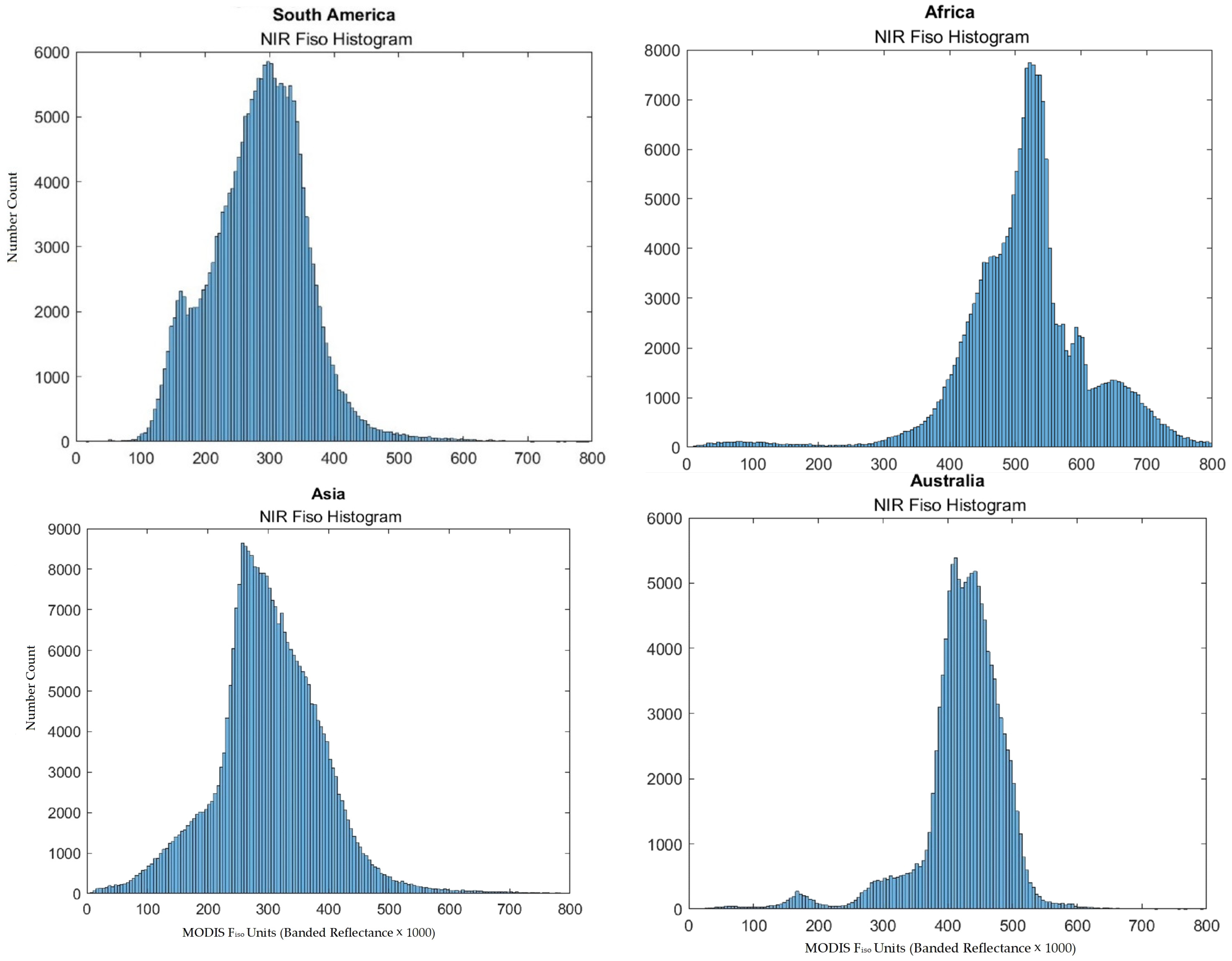
As stated, the IGBP system has fourteen different vegetation classes, one snow class, a water class, an urban class (of which the latter two were unused in this experiment), and classifies everything else in a single barren class. This broad class incorporates rock, mountains, mineral deposits, different types of soils, and sand. When the MODIS product MCD12Q1 was used for reference, the barren pixels in Africa were noticeably divergent from the other continents. When analyzing these inconsistencies in barren pixels between continents in a histogram, shown in Figure 6, three distinct reflectance signatures were observed. The band chosen for this analysis was the NIR band due to its high signal level and minimal atmospheric effects. The peaks were observed to be continent dependent, and the four continents could be separated into three groups: Asia/South America, Australia, and Africa, which were defined as dark soil, light soil, and sand, respectively, shown in Figure 7. These banded reflectance values are shown in

Table 3. Average banded reflectance for barren land cover types.

IGBP	Dark	Light	Sand
Blue	0.126	0.131	0.147
Green	0.176	0.242	0.281
Red	0.248	0.354	0.441
NIR	0.291	0.437	0.529
SWIR1	0.385	0.614	0.711
SWIR2	0.371	0.506	0.664

.

3.3. Global Classification of Pixels during Underfly

One approach to analyzing Landsat underfly imagery would be to use the information gleaned from MODIS Land Cover Types and BRDF analysis as described in the preceding section. However, one major drawback to this approach is the substantial difference between the spatial extent of MODIS product pixels and Landsat pixels—500 m versus 30 m on a side. Aggregating Landsat pixels up to MODIS size would essentially combine 225 Landsat pixels into one and prevent taking advantage of Landsat’s higher spatial resolution. Thus, an approach was needed to overcome this difficulty.

3.3.1. SDSU EPICS—November Analysis

Fortunately, the Extended Pseudo Invariant Calibration Site (EPICS) activity at South Dakota State University could be used to help sort Landsat pixels based on cover type [16,17,18]. EPICS was developed to identify every potential Pseudo Invariant Calibration Site (PICS) on the planet. It analyzes every pixel in the Landsat 8 archive to do this. To accomplish this, the EPICS project analyzed all Landsat 8 data collected in November (the month of the underfly maneuver) and classified each pixel into one of 500 distinct groups based on an unsupervised k-means algorithm approach. Each k-means clustered group had a mean and standard deviation on each band that was meant to fit the spectral range of each cluster. A normalized difference vegetation index (NDVI) was then used to classify which of the 500 clusters were vegetative clusters. The k-means average values of each cluster were used to calculate an NDVI using Equation (1) and if the NDVI value of a cluster exceeded 0.2 that cluster was classified as vegetative. A threshold of 0.2 was used because USGS states that NDVI values of 0.2 and greater correspond to grasslands and areas of thicker vegetation [19]. The familiar NDVI expression is

$$\mathrm{NDVI}=\frac{{\mathrm{R}}_{\mathrm{NIR}}-{\mathrm{R}}_{\mathrm{Red}}}{{\mathrm{R}}_{\mathrm{NIR}}+{\mathrm{R}}_{\mathrm{Red}}}$$

(1)

where R is the reflectance of the NIR and red spectral bands of Landsat 8.

An approach like the NDVI classification was used to find which of the clusters were soil using the bare soil index (BSI) and a threshold of 0.021. Diek et al., 2017, state that values greater than 0.021 using this BSI equation are considered bare soil [20]. Using Equation (2), the BSI value of each cluster was calculated using

$$\mathrm{BSI}=\frac{({\mathrm{R}}_{\mathrm{SWIR}2}+{\mathrm{R}}_{\mathrm{Red}})-\left({\mathrm{R}}_{\mathrm{NIR}}+{\mathrm{R}}_{\mathrm{Blue}}\right)}{\left({\mathrm{R}}_{\mathrm{SWIR}2}+{\mathrm{R}}_{\mathrm{Red}}\right)+\left({\mathrm{R}}_{\mathrm{NIR}}+{\mathrm{R}}_{\mathrm{Blue}}\right)}$$

(2)

where R is the reflectance of the SWIR2, NIR, red, and blue spectral bands of Landsat 8.

3.3.2. Global Classification of Pixels Procedure

To compare IGBP land cover types to the EPICS cluster cover types, each of the vegetative and soil clusters, as defined from the BSI and NDVI metrics, respectively, were forced into an IGBP cover-type classification. For all the soil and vegetative classes, the spectral means for the blue band through the SWIR-2 band were compared to the isotropic variable averages of each IGBP cover type. The IGBP cover type that yielded the smallest overall difference was the classification that the cluster was sorted into.

During the underfly maneuver, the USGS EROS archive was monitored hourly and available scene pairs (Landsat 8 and Landsat 9) with overlapping pixels were immediately extracted from the archive. This continued for two weeks after the underfly event, as scenes were still being added to the archive. Image pairs were processed according to the following procedure.

• Overlap regions were identified in the scene pairs.
• To ensure only homogeneous regions were processed, edges in the imagery were detected with the Canny edge detector [21].
• To further ensure that edges were avoided, each edge detected in the previous step was dilated by one pixel on either side.
• Each pixel within homogeneous regions was then classified as described previously into an IGBP class. Three IGBP class types had no matching clusters: evergreen needleleaf trees, deciduous broadleaf trees, and closed shrublands.
• There were 150 clusters out of the 500 that did not meet the NDVI or BSI thresholds (vegetation and soil). Out of these clusters, snow pixels were classified using the BQA band, and water pixels were used in the TIRS bands. Any pixels not falling into these categories were rejected.
• For each pixel pair, the cross-calibration ratio (L8/L9) was calculated.
• For each scene pair, data were aggregated according to IGBP land cover type and spectral band. The following scene-based statistics were gathered: cross-calibration ratio min, mean, max and standard deviation values; min, mean, max and standard deviation for Landsat 8 and 9 reflectance levels; VAAD min, mean, and max values; VZAD (rounded into 0.25° bins); as well as WRS-2 path/row values.

3.4. Analysis of Bands 8–11

The panchromatic band, band 8, has a spatial resolution of fifteen meters compared to the thirty-meter resolution of the rest of the OLI bands. For every scene pair, this resampling was required for all the BQA and viewing angle files for the underfly scenes to match the band 8 resolution. As there is warping towards the edge of scenes, when the UTM file was read in and reprojected across multiple path/rows, the band 8 images would sometimes have an extra pixel along the edges. This presented problems with the pixel extraction and, therefore, the filtering process. This was mitigated by only referencing image pairs that had the same path/row, so map reprojection would not be needed; however, this limited the range of possible VZAD values to ±4°.

Since the cirrus band, band 9, is used mostly for cirrus cloud detection, and is centered at 1.37 µm, the ground is normally undetectable due to signal absorption by the atmosphere. Thus, a cross-calibration of band 9 during the underfly using surface pixel pairs was impossible.

Water is an optimal surface target for thermal imaging due to its homogeneous nature and well-behaved emissivity properties, so the TIRS bands 10 and 11 cross-calibration was calculated only using the water pixels found in the same images as land pixels, since no pure ocean scenes were captured. The BQA was used to extract water pixels from each scene. These data included coastal ocean pixels, lakes, and rivers. Pixel values in these bands are only in radiance units, while bands 1–8 employed both radiance and reflectance units.

4. Results

As stated in Section 2 of this paper, spectral uncertainty was determined to be minimal due to the similar nature of each sensor’s spectral bandpasses. Due to this, a spectral band adjustment factor was not applied in these initial results. However, from the uncertainty analysis above, the judicious use of vegetative pixel pairs could be used to reduce uncertainty in the green and red bands. As was also discussed, pointing uncertainty was also addressed as experts at USGS EROS indicated the geometric accuracy would be highly similar between the instruments, to within five meters for most scene pairs: essentially negligible for this calibration. This left angular uncertainty in the form of the BRDF effect being the last major source of uncertainty to address. BRDF modelling showed that the view zenith angle had the largest effect on the observed reflectance difference between two sensors, which proved to be the driving factor for uncertainty reduction during this data analysis.

4.1. Outlier Reduction

Based on analysis of the Landsat 7 and Landsat 8 underfly, there was strong potential for outliers with the consequent need for an outlier-rejection approach. As stated earlier, the data were grouped based on land cover types. The key parameter was top-of-atmosphere reflectance, and the minimum, maximum, average, and standard deviation reflectance values for Landsat 8 and 9 were calculated per pixel for each scene pair. The mean reflectance values were used to find the ratio mean of Landsat 8 to Landsat 9 (L8/L9). This ratio, when applied to the Landsat 9 reflectance value, is the gain value to cross-calibrate the sensor to Landsat 8 for that scene and land cover type. Finding an optimal cross-calibration gain estimate across all scenes and land cover types required some filtering to remove outliers.

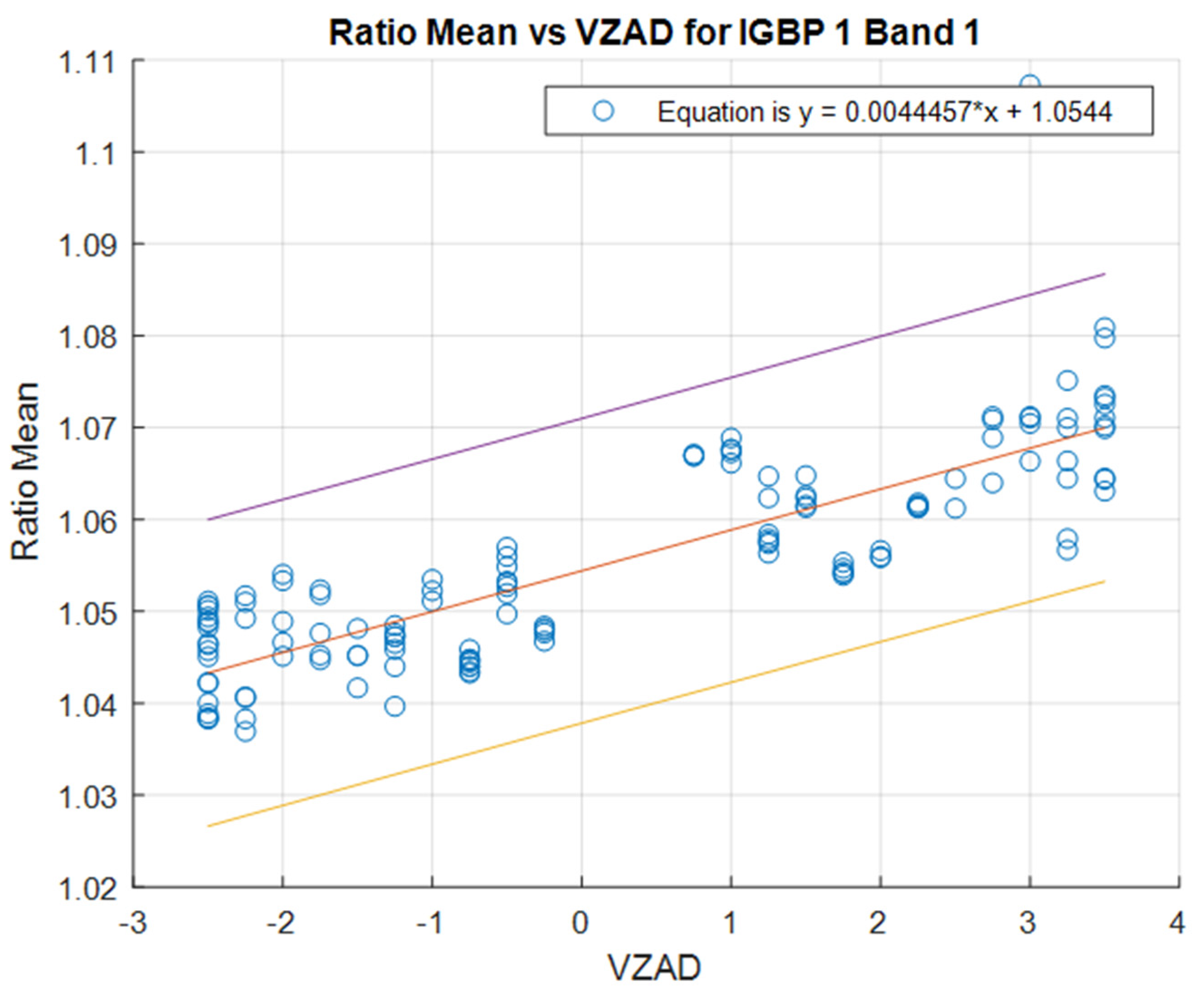
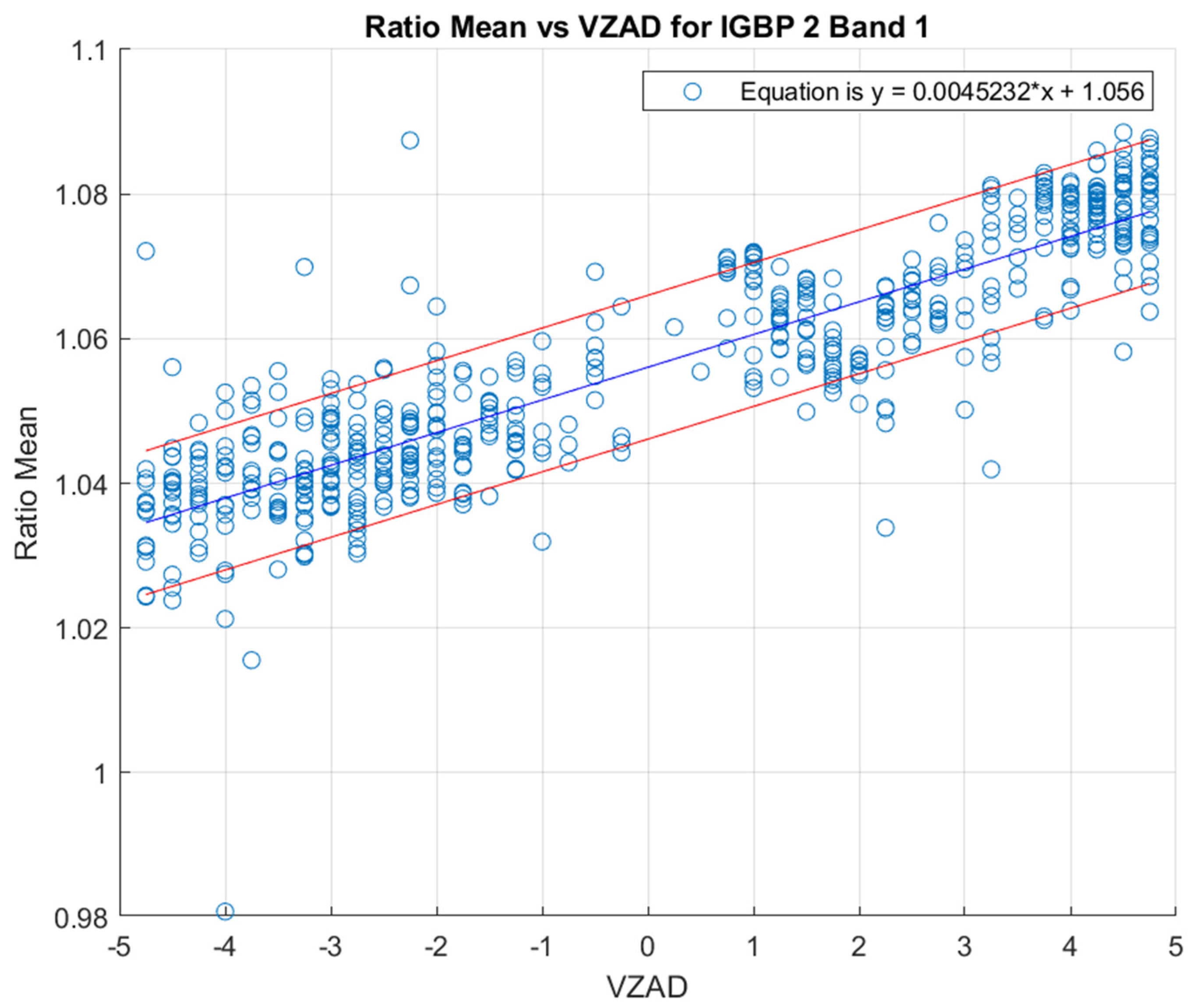
Once all the homogeneous land cover data were extracted from each scene, five parameters were modified to filter out outliers and optimize cross-calibration results: VZAD range, minimum pixel number, signal level, signal standard deviation, and VAAD range. The calibration ratio mean between Landsat 8 and 9 increased as the relative view zenith angle between the sensors also increased, as predicted by the BRDF modeling described previously. Therefore, this parameter was chosen as a primary method for the filtering algorithm, as shown in Figure 8. Every pixel in a Landsat scene has a corresponding view angle. For underfly scene pairs, there is a corresponding difference in view angle (VZAD) for each pixel pair. When plotting ratio mean against VZAD, the effect of BRDF is observed and is quite linear, as shown in Figure 8. After removing outliers from these data, the zero intercept becomes an accurate estimate of the cross-calibration gain of the two sensors.

Scene pairs with very few pixels of certain land cover types were determined to statistically bias the overall ratio mean, so a minimum pixel-number threshold parameter was also added as a filter step; this threshold was usually set to a minimum of 10,000 pixels in a scene. This eliminated errant values that were due to an insufficient number of observations. Through various tests, this parameter was determined to have a relatively large effect on the overall standard deviation of the ratio mean, with higher thresholds tending to generate lower variability.

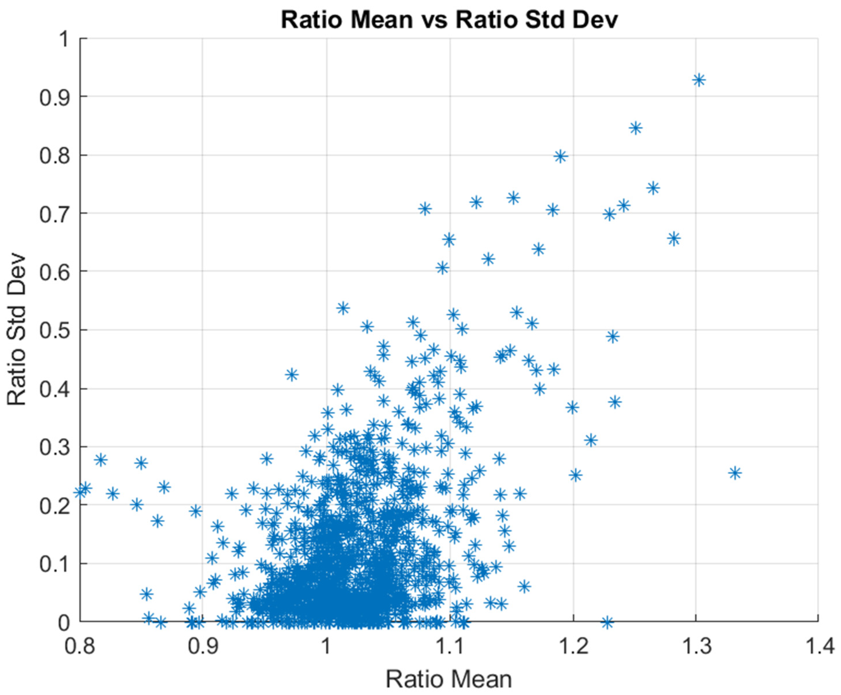
A reflectance signal level range parameter was implemented to limit values to what would be expected at each wavelength for each land cover type. Through various tests, this parameter was determined to not significantly influence cross-calibration values, so the main adjustment applied was removing the noise floor by limiting the minimum reflectance value to 0.01. The accuracy of the underfly method is based on limiting estimates to only uniform regions within the imagery. Thus, when a particular scene produced large standard deviations for the ratio mean, this would typically bias the estimate, as shown in Figure 9. Therefore, a data-driven threshold to limit the standard deviation of the ratio mean to less than 0.2 was implemented.

Finally, the relative angular difference between the solar azimuth and each of the sensors’ view azimuth was implemented as a parameter and quantified as the view azimuth angle difference (VAAD). This parameter was applied when analysis regarding angular differences showed that the further away the sensors were from the principal plane of the sun with respect to azimuth angle, the less the BRDF effect was observed. This is due to a “hot spot” occurring along the principal plane when observed on the BRDF model for many land cover types. As previously mentioned, the sensor is on the principal plane when it is in the same azimuth plane as the sun relative to the target, while it is on the cross-principal plane when it is orthogonal to the principal plane. Each sensor had its own VAAD, which was filtered on a scale of 0 to 90 degrees, with 0 indicating that the sensor was directly on the principal plane and 90 indicating the sensor was directly on the cross-principal plane. While the solar azimuth angle for each scene pair should be almost identical due to the small temporal difference between Landsat 8 and 9, the view azimuth angle of each sensor differed significantly during the underfly period. BRDF modelling showed that the ratio mean vs. VZAD slope was lower the closer the sensor was to the cross-principal plane. However, analysis showed that the VAAD did not greatly affect the VZAD intercept at 0°. Due to this, the VAAD parameter was not used in the filtering algorithm.

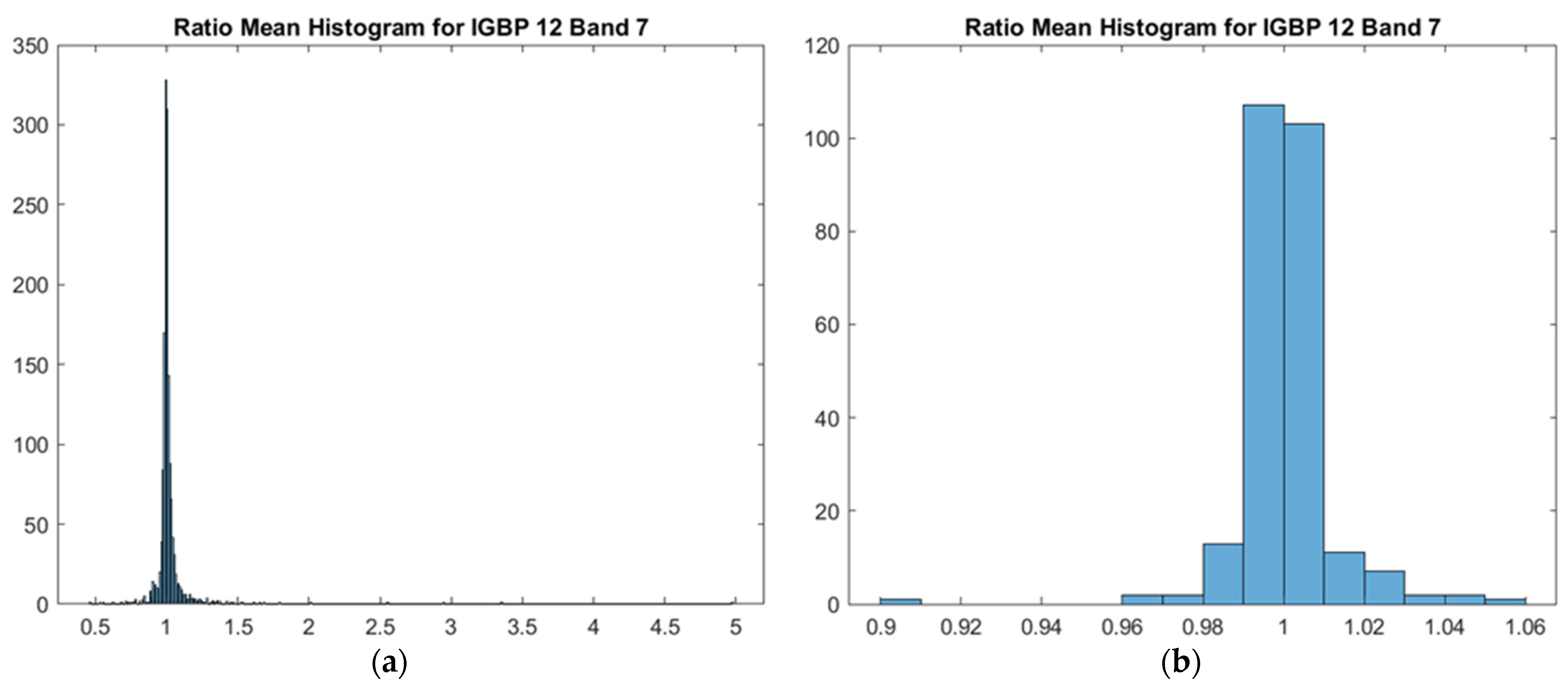
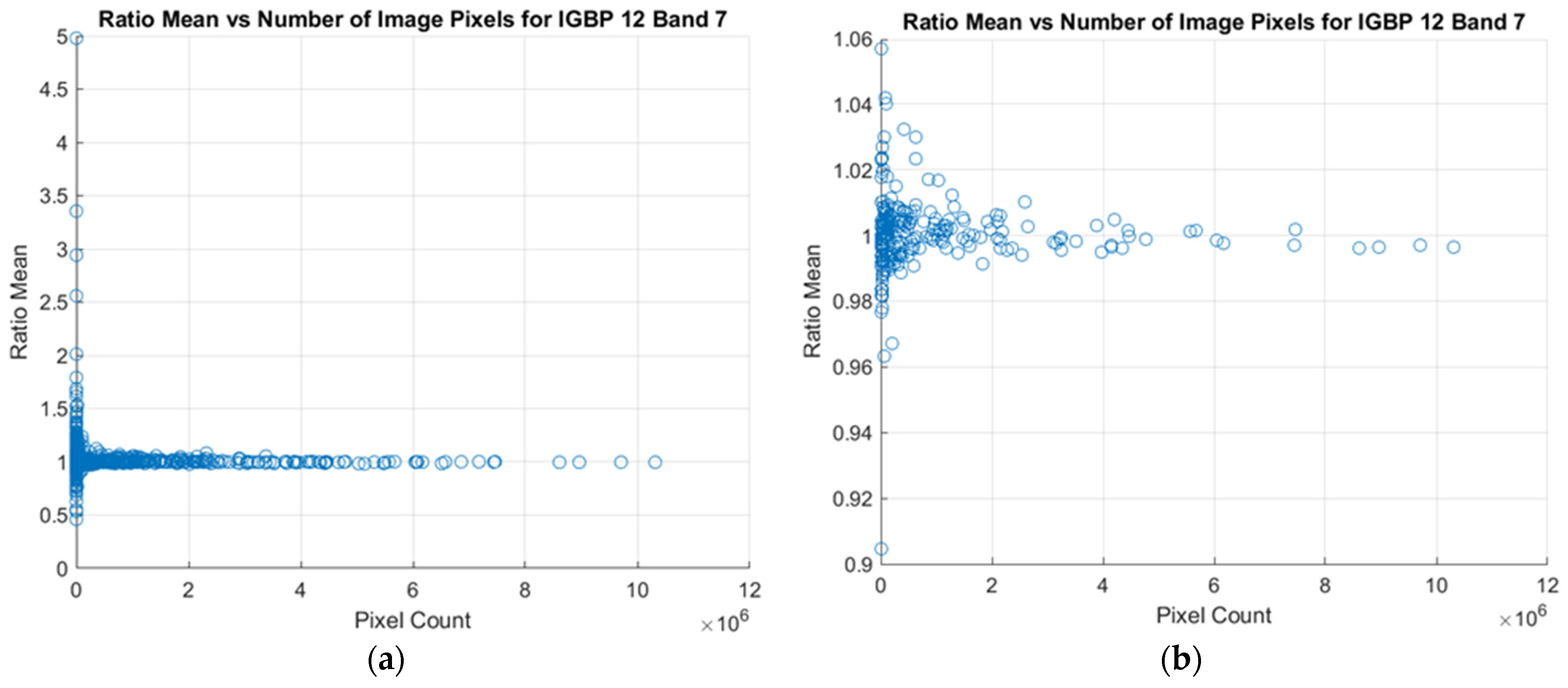
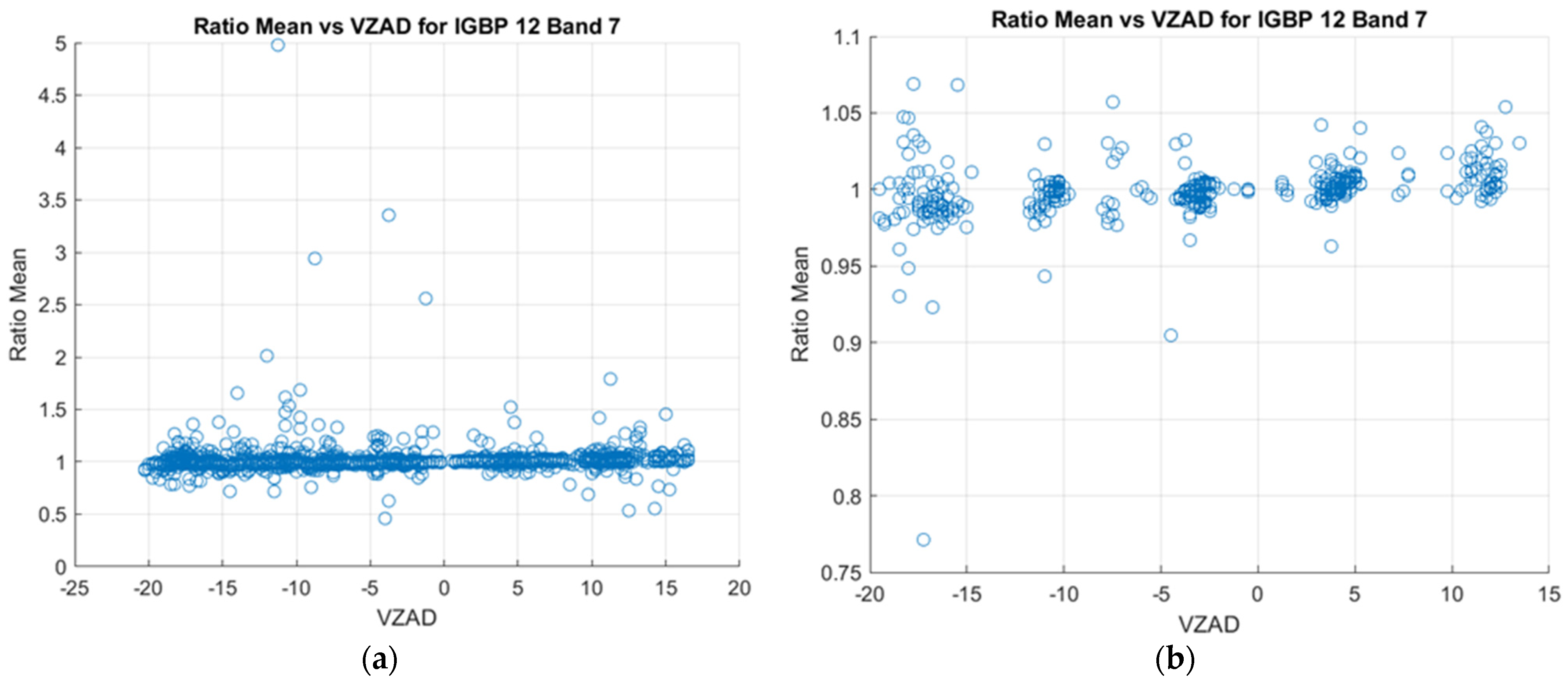
All of these parameter filters were applied to the data with the result that outliers were largely rejected, as shown in Figure 10, Figure 11 and Figure 12. Each of these figures show data before and after outlier rejection. In Figure 10, the left panel illustrates a histogram for ratio mean, IGBP 12, band 7, before filtering where outliers exist from essentially zero to a value of five. In the right panel, after outlier rejection, all data range from 0.90 to 1.06. Figure 11 illustrates ratio mean as a function of the number of pixels within a scene. Note the scatter for small numbers of pixels along the vertical axis of the left plot. After outlier rejection, in the right panel, the data have been substantially reduced and lie from 0.90 to 1.06. Figure 12 illustrates outlier rejection for ratio mean versus VZAD. In all cases, the central tendency of the data remained unchanged while the variability in the distribution was dramatically decreased.

As can be seen in the above figures, parameter filtering reduced the effect outliers had on the data, which reduced overall uncertainty for cross-calibration. However, an accurate estimator was needed to determine a final cross-calibration gain value for each band.

4.2. Cross-Calibration Ratio Estimators

Estimates with corresponding uncertainty measurements were calculated for each band per IGBP land cover type. Three estimators were considered: the filtered ratio-mean data with standard deviation as the uncertainty measurement, the median value of the data with an uncertainty quantified as the median absolute difference (MAD), and the intercept from the fitted line of VZAD plotted against the cross-calibration ratio with a 68% confidence interval used for uncertainty.

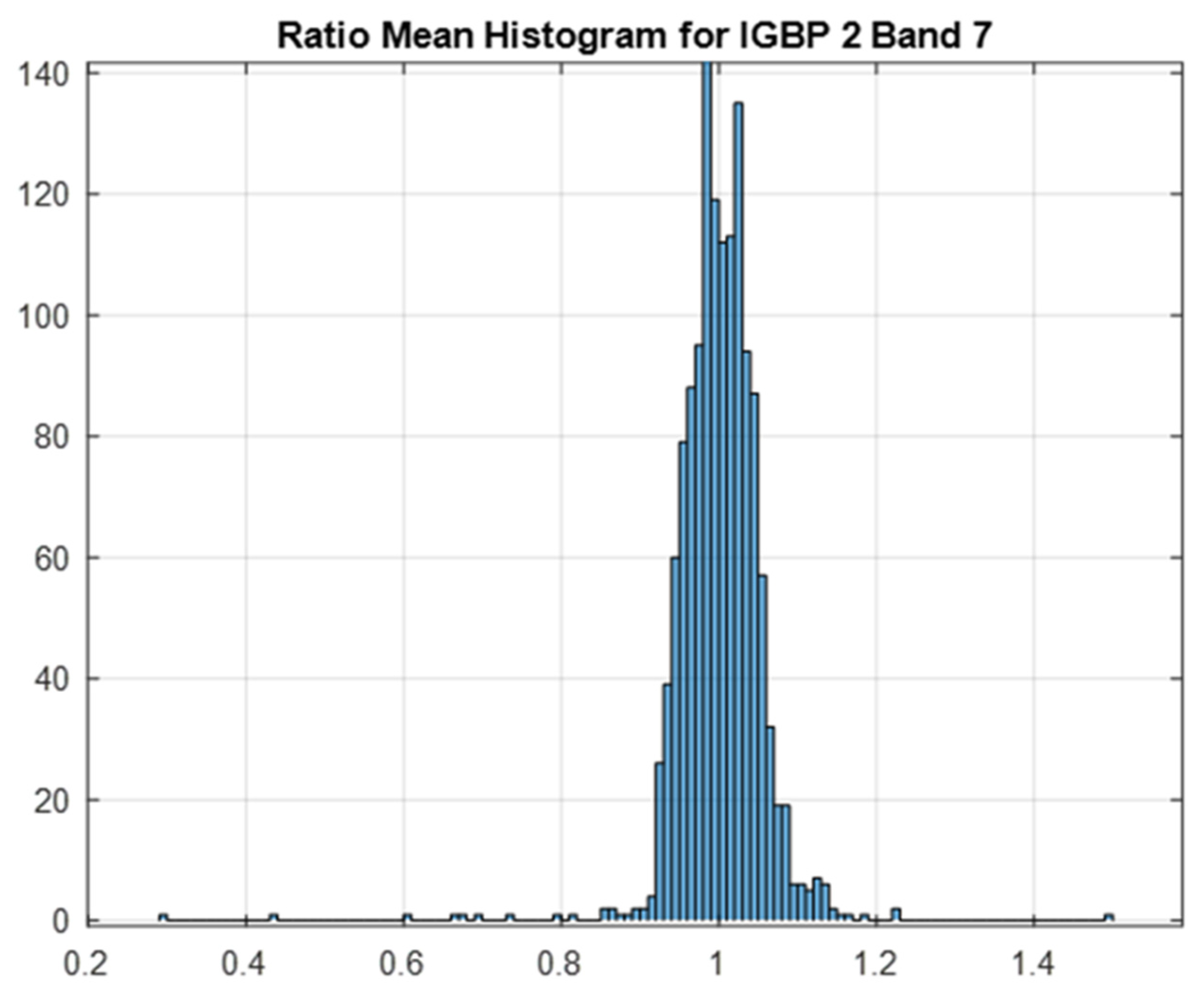
The ratio-mean estimator was the simplest estimator but had several disadvantages. The ratio values tended to increase as VZAD increased; this leads to a large uncertainty estimate. The data used to estimate the cross-calibration value in some cases was not symmetrical with respect to VZAD; therefore, if there was an imbalance of data, the cross-calibration accuracy would be biased. For example, if there was more data with respect to a positive VZAD, then the result would skew in that direction. When the ratio-mean values were plotted using a histogram, asymmetrical “heavy-tailed” data distributions showed the bias of this estimator, which could be influenced by outliers even after outlier filters were applied, as shown in Figure 13. In the case of this estimator, the sample standard deviation was used as the uncertainty measurement.

Due to the nature of order statistics, a ratio-median estimator is more immune to outliers than a ratio-mean estimator. However, the median estimator still had its drawbacks. There was an absence of data at 0° VZAD due to the critical period of the underfly (when the sensors were almost perfectly aligned) occurring over the ocean, which meant no data was collected. Note that the sensors did not have to be at nadir viewing to obtain the true cross-calibration value, they just needed the same view zenith angle for a given pixel pair. If a median estimator were to be used, the estimated cross-calibration gain value supposedly linked to 0° VZAD quite possibly would still be biased due to a lack of data at that view angle. The uncertainty measurement for this estimator was the MAD, which is a more-robust statistic than standard deviation, again due to its statistical resilience to outliers.

The final estimator considered used the VZAD intercept to estimate the cross-calibration value. This was found by calculating a linear fit equation for the filtered data, and the intercept of that line at 0° VZAD was used as the estimator, all of which are shown in Figure 14. This approach would not be nearly as affected by the lack of data at VZAD = 0°, since the estimated value would approximate what occurred at that angle. Since the two sensors could be in different path/rows and still see the same pixels, data were captured with VZADs up to ±20°, which would give a wide range of data for the linear fit equation. The VZAD intercept value also benefitted from the fact that it would essentially remove the BRDF effect expected from VZAD, as it would estimate the value if the sensors were perfectly aligned. However, this approach would still be prone to the same problem as the mean estimator if there was an imbalance across the VZAD 0° axis. If there were more data on the positive VZAD axis, results could be skewed in that direction. The VZAD filter was helpful in this case and could balance the data accordingly. The uncertainty measurement used for this estimator was a 68% confidence interval, as shown in Figure 14, which represents a confidence of one standard deviation that a given value will fall within the range above or below the linear fit equation defined by the confidence interval.

The mean, median, and VZAD intercept estimators all had comparable cross-calibration values, with the main difference between them being the uncertainty measurement. The VZAD intercept estimator was ultimately chosen for several reasons. One was that it had the lowest uncertainty measurement of the three, with its 68% confidence interval being smaller than the mean standard deviation and the median absolute difference. This likely came from the lack of VZAD at zero data, so the VZAD intercept was best-suited for approximating that value. It was also felt that the VZAD intercept approach was the least subject to bias of the three estimators. Lastly, the biggest benefit was that uncertainty caused by the BRDF effect with respect to view zenith angle was effectively cancelled out due to the value being estimated at a nadir.

4.3. Initial Calibration Estimates

Due to data-driven biases that occurred with traditional mean and median estimators, the VZAD estimator was utilized exclusively for the cross-calibration of Landsat 9. Data filtering based on parameter thresholds was implemented with specific values listed in Appendix A,

Table A1. Vegetation-filtering algorithm parameters.

Parameters	Deciduous Needleleaf	Mixed Forests	Open Shrublands	Woody Savannas	Savannas	Grasslands	Cropland	Natural Vegetation	Evergreen Broadleaf
Min VZAD	−10	−10	−10	−10	−10	−10	−10	−10	−10
Max VZAD	10	10	10	10	10	10	10	10	10
Min VAAD L8	0	0	0	0	0	0	0	0	0
Min VAAD L9	0	0	0	0	0	0	0	0	0
Min # of Pixels	10,000	1000	10,000	10,000	10,000	10,000	10,000	5000	5000
Min Reflectance L8	0.01	0.01	0.01	0.01	0.01	0.01	0.01	0.01	0.01
Max Reflectance L8	1	1	1	1	1	1	1	1	1
Min Reflectance L9	0.01	0.01	0.01	0.01	0.01	0.01	0.01	0.01	0.01
Max Reflectance L9	1	1	1	1	1	1	1	1	1
Min Std Dev L8	0	0	0	0	0	0	0	0	0
Max Std Dev L8	1	1	1	1	1	1	1	1	1
Min Std Dev L9	0	0	0	0	0	0	0	0	0
Max Std Dev L9	1	1	1	1	1	1	1	1	1
Min Std Dev of Ratio	−1	−1	−1	−1	−1	−1	−1	−1	−1
Max Std Dev of Ratio	0.2	0.2	0.2	0.2	0.2	0.2	0.2	0.2	0.2

for vegetative cover and

Table A2. Barren-filtering algorithm parameters.

Parameters	Dark Soil	Light Soil	Sand
Min VZAD	−10	−10	−10
Max VZAD	10	10	10
Min VAAD L8	0	0	0
Min VAAD L9	0	0	0
Min # of Pixels	10,000	10,000	1000
Min Reflectance L8	0.01	0.01	0.01
Max Reflectance L8	1	1	1
Min Reflectance L9	0.01	0.01	0.01
Max Reflectance L9	1	1	1
Min Std Dev L8	0	0	0
Max Std Dev L8	1	1	1
Min Std Dev L9	0	0	0
Max Std Dev L9	1	1	1
Min Std Dev of Ratio	−1	−1	−1
Max Std Dev of Ratio	0.2	0.2	0.2

for barren land cover. Note that the threshold on minimum pixel value was reduced when small amounts of particular vegetation types were imaged. Land cover types were aggregated into two major subsets: vegetative and barren. This was driven by concerns regarding bias due to spectral differences and the more Lambertian properties of barren surfaces. As mentioned previously, the barren cover type was further divided into three categories: dark soil, light soil, and sand. Unfortunately, not enough data was collected over snow and ice to make this land cover type a useful category. Mean values of the cross-calibration ratio were calculated for each cover type and each band, along with the standard deviation of the data. These are listed in

Table 4. Barren land cover types cross-calibration gain reflectance values.

	Dark Soil		Light Soil		Sand
	Mean	±σ	Mean	±σ	Mean	±σ
Band 1	1.056	0.015	1.055	0.014	1.056	0.014
Band 2	1.050	0.016	1.050	0.013	1.050	0.007
Band 3	1.039	0.017	1.040	0.014	1.041	0.007
Band 4	1.032	0.014	1.031	0.014	1.032	0.008
Band 5	1.021	0.015	1.021	0.013	1.021	0.008
Band 6	0.994	0.015	0.993	0.013	0.994	0.011
Band 7	1.001	0.016	1.000	0.012	1.000	0.012
Band 8	1.025	0.008	1.025	0.012	1.027	0.008

and

Table 5. Vegetation land cover types cross-calibration reflectance values.

	Deciduous Needleleaf		Mixed Forests		Open Shrublands		Woody Savannas		Savannas
	Mean	±σ	Mean	±σ	Mean	±σ	Mean	±σ	Mean	±σ
Band 1	1.056	0.011	1.056	0.011	1.054	0.009	1.056	0.010	1.056	0.010
Band 2	1.051	0.012	1.050	0.012	1.050	0.009	1.051	0.012	1.051	0.011
Band 3	1.035	0.014	1.032	0.014	1.038	0.009	1.034	0.014	1.036	0.014
Band 4	1.033	0.016	1.032	0.017	1.031	0.008	1.033	0.017	1.033	0.015
Band 5	1.025	0.014	1.023	0.013	1.021	0.007	1.024	0.014	1.023	0.014
Band 6	0.997	0.018	0.996	0.017	0.993	0.007	0.997	0.018	0.996	0.014
Band 7	1.007	0.016	1.005	0.019	0.999	0.007	1.005	0.019	1.003	0.014
Band 8	1.016	0.018	1.018	0.018	1.025	0.009	1.020	0.016	1.020	0.012
	Grasslands		Cropland		Natural Vegetation		Evergreen Broadleaf
	Mean	±σ	Mean	±σ	Mean	±σ	Mean	±σ
Band 1	1.055	0.014	1.055	0.011	1.057	0.010	1.056	0.011
Band 2	1.051	0.014	1.051	0.012	1.052	0.010	1.050	0.012
Band 3	1.038	0.016	1.037	0.014	1.037	0.012	1.031	0.014
Band 4	1.033	0.015	1.032	0.014	1.036	0.015	1.031	0.018
Band 5	1.033	0.015	1.022	0.013	1.026	0.012	1.024	0.015
Band 6	0.995	0.013	0.995	0.013	0.998	0.013	0.994	0.017
Band 7	1.001	0.013	1.001	0.012	1.005	0.012	1.005	0.019
Band 8	1.023	0.010	1.022	0.012	1.021	0.013	1.016	0.017

.

Table 4 lists the barren land cover type according to three categories and for each OLI spectral band. The mean values across the dark soil, light soil, and sand categories are extremely consistent with each other, with a maximum extreme spread of 0.002. The standard deviation for these data, typically in the range of 0.007 to 0.017, clearly indicates that the mean values of the three categories are indistinguishable from one another and can be aggregated into a single cross-calibration estimate.

Table 5 lists cross-calibration gain as a function of nine vegetative cover types for each OLI band. Again, mean values of all underfly data processed are listed along with the standard deviation of the data. Although one would typically expect more variability across such a wide array of vegetation types, the mean value of the cross-calibration estimates is surprisingly consistent—the extreme spread is less than 0.01 in all bands. The open-shrub land cover type produces the smallest standard deviation across vegetative cover types, averaging 0.008, while the rest of the cover types produced essentially the same value of approximately 0.015.

Comparison of the results in Table 4 and Table 5 indicate excellent consistency between barren surface-based cross-calibration gain estimates and vegetative-based estimates. The largest difference when considering the mean value for each band across both sets of data is 0.005. Since uncertainties in those estimates, as indicated by the standard deviations listed in the tables, are on the order of 0.015, it is clear that the two groups of estimates are statistically indistinguishable. However, across all land cover types, the barren types and the open-shrub type produce estimates that are extremely consistent with each other and with lower uncertainty. Due to the differences in uncertainty, the approach used to combine estimates across all land cover types into a single recommendation for the cross-calibration was the inverse-variance weighting method [22]. This approach, rather than averaging all estimates together equally, weights each estimate by the inverse of its uncertainty (variance) and is an optimal method for minimizing uncertainty. The inverse-variance weighted average can be calculated as

$$\widehat{\mathrm{y}}=\frac{{{\displaystyle \sum }}_{\mathrm{i}}\frac{{\mathrm{y}}_{\mathrm{i}}}{{\mathsf{\sigma }}_{\mathrm{i}}^2}}{{{\displaystyle \sum }}_{\mathrm{i}}\frac{1}{{\mathsf{\sigma }}_{\mathrm{i}}^2}}$$

(3)

where y_i is the ratio mean of each cover type and σ_i is the σ of each cover type. The standard deviation of this weighted average is given as

$$\mathrm{Var}\left(\hat{\mathrm{y}}\right)=\frac{1}{{{\displaystyle \sum }}_{\mathrm{i}}\frac{1}{{\mathsf{\sigma }}_{\mathrm{i}}^2}}$$

(4)

with the mean and standard deviation results given in

Table 6. Weighted variance estimator—reflectance.

	Mean	Std. Dev.
Band 1	1.056	0.003
Band 2	1.051	0.003
Band 3	1.037	0.003
Band 4	1.032	0.004
Band 5	1.021	0.001
Band 6	0.995	0.004
Band 7	1.002	0.004
Band 8	1.023	0.003

.

Table 6 shows that the cross-calibration of Landsat 9 to Landsat 8, derived from the initial prelaunch calibration of Landsat 9, was only off by 6%. Band 1 showed the largest difference, of 5.6%, while bands 6 and 7 were less than 0.5% off. Furthermore, the uncertainty of this initial evaluation of the underfly data appears to be on the order of 0.5% across all bands. These results vary slightly from those given to USGS EROS at the end of OIV: the green band recommended value was 1.040. This was the estimate derived from the barren land cover type and would not include errors from spectral differences when observing vegetative targets.

The above calculations were completed for the cross-calibration reflectance values. Since Landsat products are provided in both units of reflectance and radiance, the same process was performed on Landsat 8/9 radiance values, and the initial estimates are shown in

Table 7. Weighted variance estimator—radiance.

	Mean	Std. Dev.
Band 1	1.020	0.005
Band 2	1.000	0.005
Band 3	0.987	0.006
Band 4	1.003	0.007
Band 5	1.027	0.007
Band 6	0.998	0.010
Band 7	1.004	0.011
Band 8	1.006	0.003
Band 10	0.932	0.009
Band 11	0.954	0.008

. The TIRS bands are also shown in the table below and are based on the radiance values of water pixels found in scenes that include lakes, rivers, and coasts. As calibration in radiance space carries additional uncertainties that are not present in reflectance space, uncertainties in Table 7 are up to 1.1% (Band 7).

The initial cross-calibration ratio values were applied to the underfly data CPF files by USGS EROS and all underfly data were reprocessed. To validate that the cross-calibration was successful, the same process as shown in the methodology and results sections was performed on this reprocessed data to determine how consistent the two sensors were. The results of this validation process are shown in

Table 8. Cross-calibration validation results. Note bands 10 and 11 were not calibrated in reflectance space.

	Underfly Reprocessed Radiance Ratios		Underfly Reprocessed Reflectance Ratios
	Mean	Std. Dev.	Mean	Std. Dev.
Band 1	1.000	0.003	1.000	0.004
Band 2	1.000	0.005	1.002	0.004
Band 3	0.999	0.003	0.999	0.005
Band 4	0.997	0.003	1.000	0.004
Band 5	0.999	0.006	1.001	0.003
Band 6	0.997	0.005	1.001	0.004
Band 7	0.996	0.005	1.000	0.004
Band 8	1.001	0.005	1.004	0.003
Band 10	0.997	0.009
Band 11	1.008	0.008

.

As shown in the table above, the sensors are within 0.2% from unity, with an uncertainty within 0.5% for all bands in reflectance space. The radiance validation values are less than 0.5% from unity and below 1% in uncertainty for the OLI bands. The TIRS bands are within 1% of unity with less than 1% uncertainty. The values in the table are very nearly 1 for the OLI bands, which proves the effectiveness of the cross-calibration approach explained in this paper.

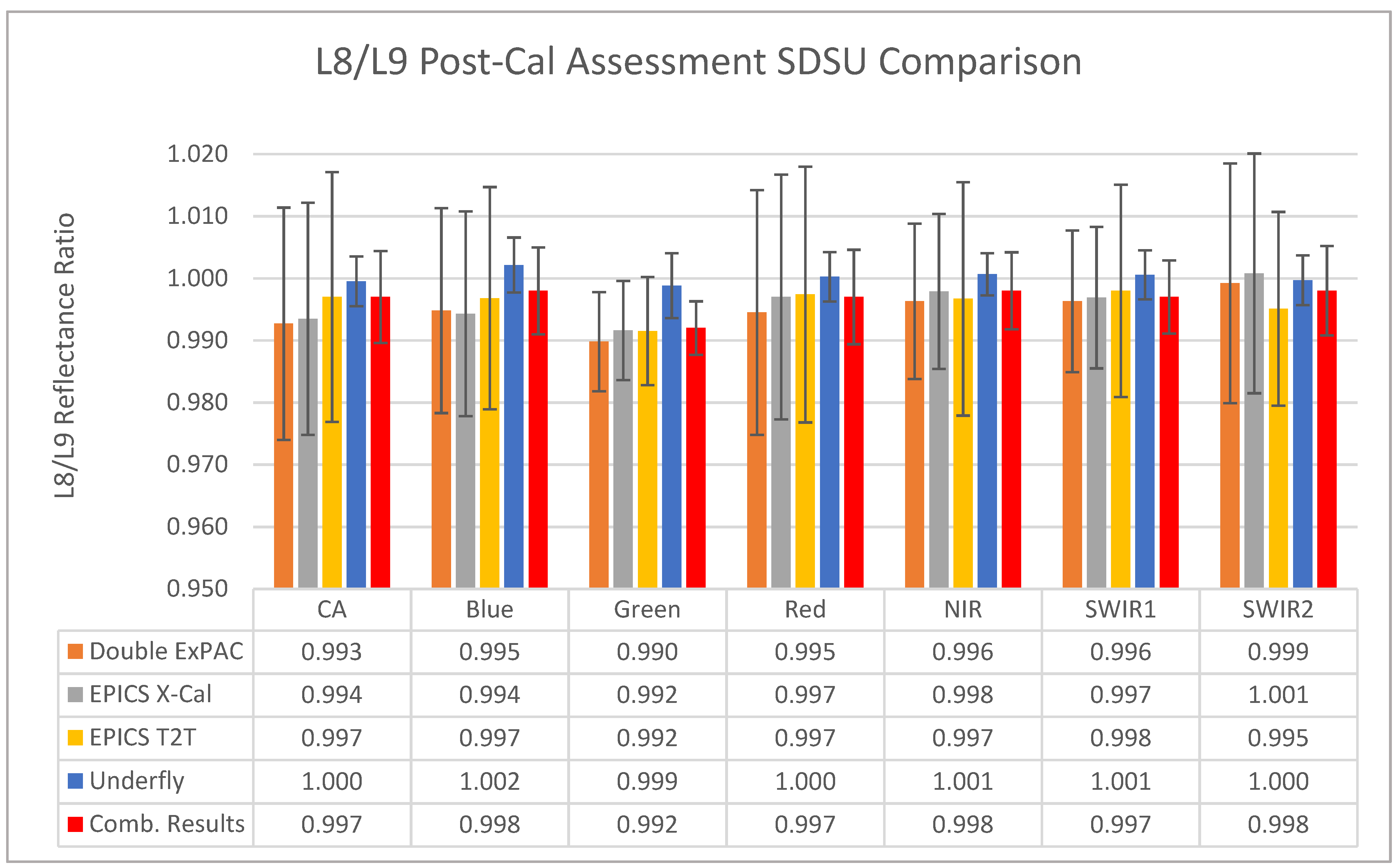
As part of the Landsat Cal/Val team, the SDSU Image Processing Lab also validated the reflectance results. Their approaches all involved Extended Pseudo Invariant Calibration Sites (EPICS). The methods used were EPICS Trend-to-Trend (T2T) [23], Traditional EPICS Cross-Calibration [16], and Double Extended-PICS Absolute Calibration (ExPAC) [16]. The EPICS techniques are used to analyze the sensors over an extended period of time to evaluate the calibration, much longer than the weeklong underfly period. Confirming the underfly results with the results of these other long-term methods over stable sites show the validity of the cross-calibration approach described in this paper. As shown in Figure 15, all methods agree that the sensors are cross-calibrated to within 1%; combining the results of all approaches indicates the sensors agree to within 0.5%, well below the uncertainty budget of the methods. These results clearly show cross-calibration was successful and all methods agree with the underfly-based results described here.

In summary, after various filter thresholds were applied to the raw underfly data to reduce outliers, an estimator was implemented to quantify the cross-calibration value of each band. This estimator used the intercept of the VZAD versus mean cross-calibration ratio linear fit equation to account for the absence of data at VZAD 0°. As a result, the major uncertainty in the process, BRDF effect due to viewing angle, is minimized. With the sources of uncertainty quantified and the most robust estimator used for analysis to further reduce uncertainty, the initial cross-calibration results have an estimated uncertainty of less than 0.5% using reflectance units and below 1% with respect to radiance. When validating the results of the cross-calibration using reprocessed underfly data with these initial ratio values applied, tests showed that the reflectance values were 0.2% within unity on average and less than 0.5% different from unity in radiance space. Validation using other approaches further confirmed the accuracy of these cross-calibration ratio values.

5. Conclusions

Landsat 9 flew underneath Landsat 8 on 11–17 November 2021, and recorded hundreds of scene pairs viewed essentially simultaneously by the two sets of instruments. As Landsat 9 instruments were essentially clones of the Landsat 8 instruments, the underfly maneuver presented a near-optimal opportunity for the cross-calibration of the two instruments. Three sources of uncertainty were investigated prior to the underfly maneuver in order to determine the level of precision possible for cross-calibration. Investigations indicated that, due to the similarities between the spectral filters of the two instruments, uncertainty due to spectral differences would be 0.2% or less in most scenarios. The only significant exception occurred with the green band for certain types of vegetation, when the uncertainty could grow to 0.5–1.0%. Pointing uncertainties were considered negligible due to the excellent geometric performance of the two spacecrafts. Unfortunately, BRDF uncertainty was significant, even though Landsat viewing zenith angles are small (<7.5° off nadir). For typical vegetative surfaces, BRDF uncertainties could reach up to 10%. Fortunately, because of the small off-nadir viewing angles, a robust estimator could be developed that essentially fits a linear model to the cross-calibration ratio as a function of difference in the view zenith angles of the two sensors.

Results indicated very robust estimates of the cross-calibration gain ratio with uncertainties on the order of 0.5%. Gain-ratio estimates were consistent across all land cover types with barren and open-shrub land covers showing better precision than the rest. As a result, within each band, estimates across all land cover types were combined based on the inverse variance weighting method. The resulting estimates showed the sensors were within 6% of each other at the short wavelengths and less than 0.5% of each other in the SWIR bands. The values given in Table 6 and Table 7 were recommended to USGS EROS for a calibration update of Landsat 9 following OIV. As stated, one exception was the green band reflectance cross-calibration value. A value of 1.040 was recommended, as it was felt that the estimate derived from the barren land cover type would not include error due to spectral differences when viewing vegetative targets in the green band. This was further supported by the lower uncertainties obtained with the barren land cover types. Interestingly, this did not occur with the green band in radiance space—uncertainties were the same for both vegetative and barren land cover types—and so the weighted variance estimate was used.

Results generated in this paper were developed during the OIV period (the first 90 days after launch). They were the most-accurate initial recommendation available at the time. A more complete analysis is ongoing at the time of this writing and will be used to update Landsat 9 calibration near the end of the first year of operation.

References

- Masek, J.G.; Wulder, M.A.; Markham, B.; McCorkel, J.; Crawford, C.J.; Storey, J.; Jenstrom, D.T. Landsat 9: Empowering open science and applications through continuity. Remote Sens. Environ. 2020, 248, 111968. [Google Scholar] [CrossRef]
- MarkhamM, B.; McCorkel, J.; Montanaro, M.; Morland, E.; Pearlman, A.; Pedelty, J.; Wenny, B.; Barsi, J.; Donley, E.; Efremova, B.; et al. Landsat 9: Mission Status and Prelaunch Instrument Performance Characterization and Calibration. In Proceedings of the IGARSS 2019—2019 IEEE International Geoscience and Remote Sensing Symposium, Yokohama, Japan, 28 July–2 August 2019; pp. 5788–5791. [Google Scholar] [CrossRef]
- Metzler, M.D.; Malila, W.A. Characterization and comparison of Landsat-4 and Landsat-5 Thematic Mapper data. Photogramm. Eng. Remote Sens. 1985, 51, 1315–1330. [Google Scholar]
- Teillet, P.M.; Markham, B.L.; Barker, J.L.; Storey, J.C.; Irish, R.R.; Seiferth, J.C. Landsat sensor cross-calibration using nearly coincidental matching scenes. In Algorithms for Multispectral, Hyperspectral, and Ultraspectral Imagery VI; SPIE: Bellingham, WA, USA, 2000; Volume 4049. [Google Scholar]
- Mishra, N.; Haque, M.O.; Leigh, L.; Aaron, D.; Helder, D.; Markham, B. Radiometric Cross Calibration of Landsat 8 Operational Land Imager (OLI) and Landsat 7 Enhanced Thematic Mapper Plus (ETM+). Remote Sens. 2014, 6, 12619–12638. [Google Scholar] [CrossRef] [Green Version]
- Teillet, P.M.; Fedosejevs, G.; Thome, K.J.; Barker, J.L. Impacts of spectral band difference effects on radiometric cross-calibration between satellite sensors in the solar-reflective spectral domain. Remote Sens. Environ. 2007, 110, 393–409. [Google Scholar] [CrossRef]
- Chander, G.; Mishra, N.; Helder, D.L.; Aaron, D.; Choi, T.; Angal, A.; Xiong, X. Use of EO-1 Hyperion data to calculate spectral band adjustment factors (SBAF) between the L7 ETM+ and Terra MODIS sensors. In Proceedings of the 2010 IEEE International Geoscience and Remote Sensing Symposium, Honolulu, HI, USA, 25–30 July 2010. [Google Scholar]
- Thenkabail, P.; Aneece, I. Global Hyperspectral Imaging Spectral-Library of Agricultural Crops for Conterminous United States V001 [Data Set]. NASA EOSDIS Land Processes DAAC, 2019. Available online: https://lpdaac.usgs.gov/products/ghisaconusv001 (accessed on 20 March 2021).
- Meerdink, S.K.; Hook, S.J.; Roberts, D.A.; Abbott, E.A. The ECOSTRESS spectral library version 1.0. Remote Sens. Environ. 2019, 230, 111196. [Google Scholar] [CrossRef]
- Baldridge, A.M.; Hook, S.J.; Grove, C.I.; Rivera, G. The ASTER Spectral Library Version 2.0. Remote Sens. Environ. 2009, 113, 711–715. [Google Scholar] [CrossRef]
- World Agroforestry (ICRAF); International Soil Reference and Information Centre (ISRIC). ICRAF-ISRIC Soil VNIR Spectral Library. In World Agroforestry—Research Data Repository, V1; World Agroforestry (ICRAF): Nairobi, Kenya, 2021. [Google Scholar] [CrossRef]
- Salvatori, R.; Salzano, R.; Franco, S.D.; Fontinovo, G.; Plini, P. SISpec 2.0 Snow-Ice Spectral Library; National Research Council of Italy, Institute of Polar Sciences: Rome, Italy, 2020.
- Wanner, W.; Li, X.; Strahler, A.H. On the derivation of kernels for kernel-driven models of bidirectional reflectance. J. Geophys. Res. Atmos. 1995, 100, 21077–21089. [Google Scholar] [CrossRef]
- Wanner, W.; Strahler, A.H.; Hu, B.; Lewis, P.; Muller, J.-P.; Li, X.; Schaaf, C.L.B.; Barnsley, M.J. Global retrieval of bidirectional reflectance and albedo over land from EOS MODIS and MISR data: Theory and algorithm. J. Geophys. Res. Atmos. 1997, 102, 17143–17161. [Google Scholar] [CrossRef] [Green Version]
- Lucht, W.; Schaaf, C.B.; Strahler, A.H. An algorithm for the retrieval of albedo from space using semiempirical BRDF models. IEEE Trans. Geosci. Remote Sens. 2000, 38, 977–998. [Google Scholar] [CrossRef] [Green Version]
- Leigh, L.; Shrestha, M.; Hasan, N.; Kaewmanee, M. Classification of North Africa for Use as an Extended Pseudo Invariant Calibration Site for Radiometric Calibration and Stability Monitoring of Optical Satellite Sensors. In Proceedings of the CALCON 2019, Utah State University, Logan, UT, USA, 19–21 September 2019. [Google Scholar]
- Shrestha, M.; Leigh, L.; Helder, D. Classification of North Africa for use as an extended pseudo invariant calibration site (EPICS) for radiometric calibration and stability monitoring of optical satellite sensors. Remote Sens. 2019, 11, 875. [Google Scholar] [CrossRef] [Green Version]
- Rueda, J.F.; Leigh, L.; Pinto, C.T.; Kaewmanee, M.; Helder, D. Classification and Evaluation of Extended PICS (EPICS) on a Global Scale for Calibration and Stability Monitoring of Optical Satellite Sensors. Remote Sens. 2021, 13, 3350. [Google Scholar] [CrossRef]
- Remote Sensing Phenology. NDVI, the Foundation for Remote Sensing Phenology. USGS, 2018. Available online: https://www.usgs.gov/special-topics/remote-sensing-phenology/science/ndvi-foundation-remote-sensing-phenology (accessed on 25 October 2021).
- Diek, S.; Fornallaz, F.; Schaepman, M.E.; De Jong, R. Barest Pixel Composite for Agricultural Areas Using Landsat Time Series. Remote Sens. 2017, 9, 1245. [Google Scholar] [CrossRef] [Green Version]
- Canny, J. A computational approach to edge detection. IEEE Trans. Pattern Anal. Mach. Intell. 1986, PAMI-8, 679–698. [Google Scholar] [CrossRef]
- Hartung, J.; Knapp, G.; Singa, B.K. Statistical Meta-Analysis with Applications; John Wiley & Sons: Hoboken, NJ, USA, 2008; pp. 44–46. [Google Scholar]
- Khakurel, P.; Leigh, L.; Kaewmanee, M.; Pinto, C.T. Extended Pseudo Invariant Calibration Site-Based Trend-to-Trend Cross-Calibration of Optical Satellite Sensors. Remote Sens. 2021, 13, 1545. [Google Scholar] [CrossRef]
Figure 1.
Representative relative spectral response (RSR) functions for OLI and OLI-2. These are band averages of 14 focal plane modules (FPMs) showing small differences.
Figure 2.
SBAFs for all OLI band averages for four common land cover types. (a) is mid-season corn, (b) is White Fir, (c) is Brazilian soil with similar results to that of a desert, and (d) is large rounded grain particles of snow.
Figure 3.
Change in cross-calibration ratio as a function of point error. These data were extracted from archived Landsat 7/8 underfly imagery and include the effects of SBAF to minimize spectral error. Thus, changes due to only pointing error will be smaller than values indicated here.
Figure 4.
(a–e): BRDF models of grass pasture for different SZA and SAA locations. Note how hot spot follows solar location. (f): Linearity of BRDF versus VZA for entire range of Landsat viewing angles.
Figure 5.
(a–e): BRDF models of Libya 4 calibration site for different SZA and SAA locations. Note how hot spot continues to follow solar location, but is more condensed than the previous figure. (f): Linearity of BRDF versus VZA for entire range of Landsat viewing angles. Note these have a smaller slope when compared to the previous figure.
Figure 6.
Banded NIR reflectance of barren classified pixels across Africa, South America, Australia, and Asia in MODIS units (reflectance × 1000). Note there are three distinct peaks in the histogram, which are continent dependent.
Figure 7.
Banded NIR reflectance of barren classified pixels separated by continent in MODIS units (reflectance × 1000). Note that South America and Asia can be grouped together to make a dark soil group, Australia into a light soil type, and Africa into a sand type.
Figure 8.
Reflectance ratio mean vs. view zenith angle difference.
Figure 9.
Ratio mean vs. ratio standard deviation. Note there is a discernable positive linear trend above a ratio standard deviation of 0.2 as the data drift to larger values.
Figure 10.
(a) Unfiltered ratio mean histogram. (b) Filtered ratio mean histogram.
Figure 11.
(a) Unfiltered ratio mean vs. number of pixels. (b) Filtered ratio mean vs. number of pixels.
Figure 12.
(a) Unfiltered ratio mean vs. VZAD. (b) Filtered ratio mean vs. VZAD.
Figure 13.
Heavy-tailed ratio mean histogram. Note there are outliers on the left side of the histogram which gives the data a slight left skew.
Figure 14.
VZAD intercept estimator. Note there are no data at 0° VZAD, but the linear fit equation compensates for that, shown in the top right of the graph. The blue line is the model while the red lines depict the 68% confidence interval.
Figure 15.
Post-calibration comparison. SDSU validated the initial cross-calibration results with multiple approaches, all showing the sensors agree to within 1%. The blue bars indicate the approach taken in this paper, with the red bars indicating the method that incorporates all of the approaches.