Article

Optimizing a Standard Spectral Measurement Protocol to Enhance the Quality of Soil Spectra: Exploration of Key Variables in Lab-Based VNIR-SWIR Spectral Measurement

1
College of Geo-Exploration Science and Technology, Jilin University, Changchun 130026, China
2
College of Surveying and Exploration Engineering, Jilin Jianzhu University, Changchun 130118, China
*
Author to whom correspondence should be addressed.
Remote Sens. 2022, 14(7), 1558; https://doi.org/10.3390/rs14071558
Submission received: 14 February 2022 / Revised: 19 March 2022 / Accepted: 22 March 2022 / Published: 23 March 2022
(This article belongs to the Special Issue Remote Sensing for Soil Organic Carbon Mapping and Monitoring)

Abstract

:
The method of proximal VNIR-SWIR (with a spectral region of 400–2500 nm) spectroscopy in a laboratory setting has been widely employed in soil property estimations. Increasing attention has been focused recently on establishing an agreed-upon protocol for soil spectral measurement, fueled by the recognition that studies carried out under different laboratory settings have made future data sharing and model comparisons difficult. This study aimed to explore the key factors in a lab-based spectral measurement procedure to provide recommendations for enhancing the spectra quality and promoting the development of the spectral measurement protocol. To this aim, with the support of the standard spectral laboratory at Jilin University, China, we designed and performed control experiments on four key factors—the light interference in the measurement course, soil temperature, soil moisture, and soil particle size—to quantify the variation in the spectra quality by the subsequent estimation accuracies of different estimation models developed with different spectra obtained from control groups. The results showed that (1) the soil–probe contact measurement derived the optimum spectra quality and estimation accuracy; however, close-non-contact measurement also achieved acceptable results; (2) sieving the soil sample into particle sizes below 1 mm and drying before spectral measurement effectively enhanced spectra quality and estimation accuracy; (3) the variation in soil temperature did not have a distinct influence on spectra quality, and the estimation accuracies of models developed based on soil samples at 20–50 °C were all acceptable. Moreover, a 30-min warm-up of the spectrometer and contact probe was found to be effective. We carried out a complete and detailed control experiment process, the results of which offer a guide for optimizing the process of laboratory-based soil proximal spectral measurement to enhance spectra quality and corresponding estimation accuracy. Furthermore, we present theoretical support for the development of the spectral measurement protocol. We also present optional guidance with relatively lower accuracy but effective results, which are save time and are low cost for future spectral measurement projects.

1. Introduction

Proximal hyperspectral spectroscopy in the visible near-infrared and shortwave infrared (VNIR-SWIR) spectral region (400–2500 nm) of soils presents a non-destructive and efficient approach for estimating numerous soil properties in a laboratory setting. The establishment and development of the calibration–validation strategy [1] for analyzing the correlation between spectra and certain physical or chemical attributes have led to the development of a spectral quantitative estimation of soil properties [2,3,4,5,6,7,8]. Despite the desired soil property estimations achieved with the proximal VNIR-SWIR hyperspectral measurement approach, a recognized limitation of this approach is the lack of a common laboratory protocol [9,10,11].
Several key variables in performing the lab-based VNIR-SWIR spectral measurement procedure on soil samples significantly influence their spectra quality and subsequent estimation accuracy to soil properties brings challenges to establish the agreed-upon protocol for soil spectral measurement [9,10,11,12,13,14]. Variability in the sample collection, sample pretreatment, laboratory environment, and the spectrometer condition may lead to significant differences in spectra quality and subsequently hamper model sharing and comparison [10,12,13,14]. Hence, investigating and optimizing the key factors in the spectral measurement procedure are essential to develop an agreed-upon protocol [15]. However, few studies have comprehensively investigated these factors, and their results have been inconsistent [15,16,17,18,19].
First, the existing VNIR-SWIR spectroscopy laboratory procedure usually requires carrying out the measurement with a high-intensity contact probe or a halogen lamp to illuminate the darkroom environment [15]. However, the different laboratory conditions and the special requirements of different operators (e.g., some laboratories prohibit the probe coming into contact with soil samples to avoid cross-contamination between samples and instruments) introduce the possibility of light interference in the measuring course. Second, soil temperature plays an important role in controlling the soil spectral characteristics [3,9]. In most cases, the spectral measurements are recommended to be carried out at room temperature [10,11,15]. However, few studies have investigated the correlation between soil temperature and corresponding spectral characteristics until now; moreover, they have not proposed a common standard [18,20]. Third, soil moisture is a major chemical chromophore that significantly influences the soil’s spectral characteristics [3,21,22,23]. The moisture variation in soil samples caused by damp environmental storage leads to significant variations in soil spectra. In most cases, studies have suggested using an air-dried or oven-dried procedure in sample pretreatment to enhance the spectral quality [9,15]; nevertheless, studies have demonstrated that in some cases the wet samples did not show significantly degraded results in spectral analysis [16,24]. Additionally, the crushing and sieving pretreatment interferes significantly with the soil texture, which generates particle size differences in soil samples. It also interferes with the radiative transfer process and further influences the soil spectral characteristic significantly [3,21,25,26]. Although previous studies have demonstrated that the spectra quality of soil samples and corresponding estimation accuracy are enhanced with fine sieving, the sieving levels that derived the optimum results differed [5,15,26,27,28].
Several reliable protocols, such as the CSIRO, TAU, CGS, and CULS [10,11,15], have been developed for standardizing the proximal VNIR-SWIR spectral measurement procedure. However, with the rise in the number of spectral measurement protocols, as well as the generation of regional and national soil spectral libraries, the variation in the generated datasets has obviously not been corrected [10]. Recent studies have attempted to standardize the spectra data obtained from different laboratory procedures into a uniform protocol from the perspective of mathematical calculation methods [10,11,15]. Nevertheless, no one has comprehensively studied unifying the key factors in the protocol from the perspective of a sample processing and spectral measurement procedure. Moreover, the requirements of existing protocols have also not been perfected in common applications because of the limitations of the laboratory environment, instrument conditions, and different operational habits [9,29,30]. Therefore, this study was carried out to investigate the variation in spectra quality and corresponding estimation accuracy generated by variations in key factors in the spectral measurement procedure with the aim of quantifying these variations. Moreover, we provide optional guidance for further proximal VNIR-SWIR spectral measurements and theoretical support for optimizing the protocols.
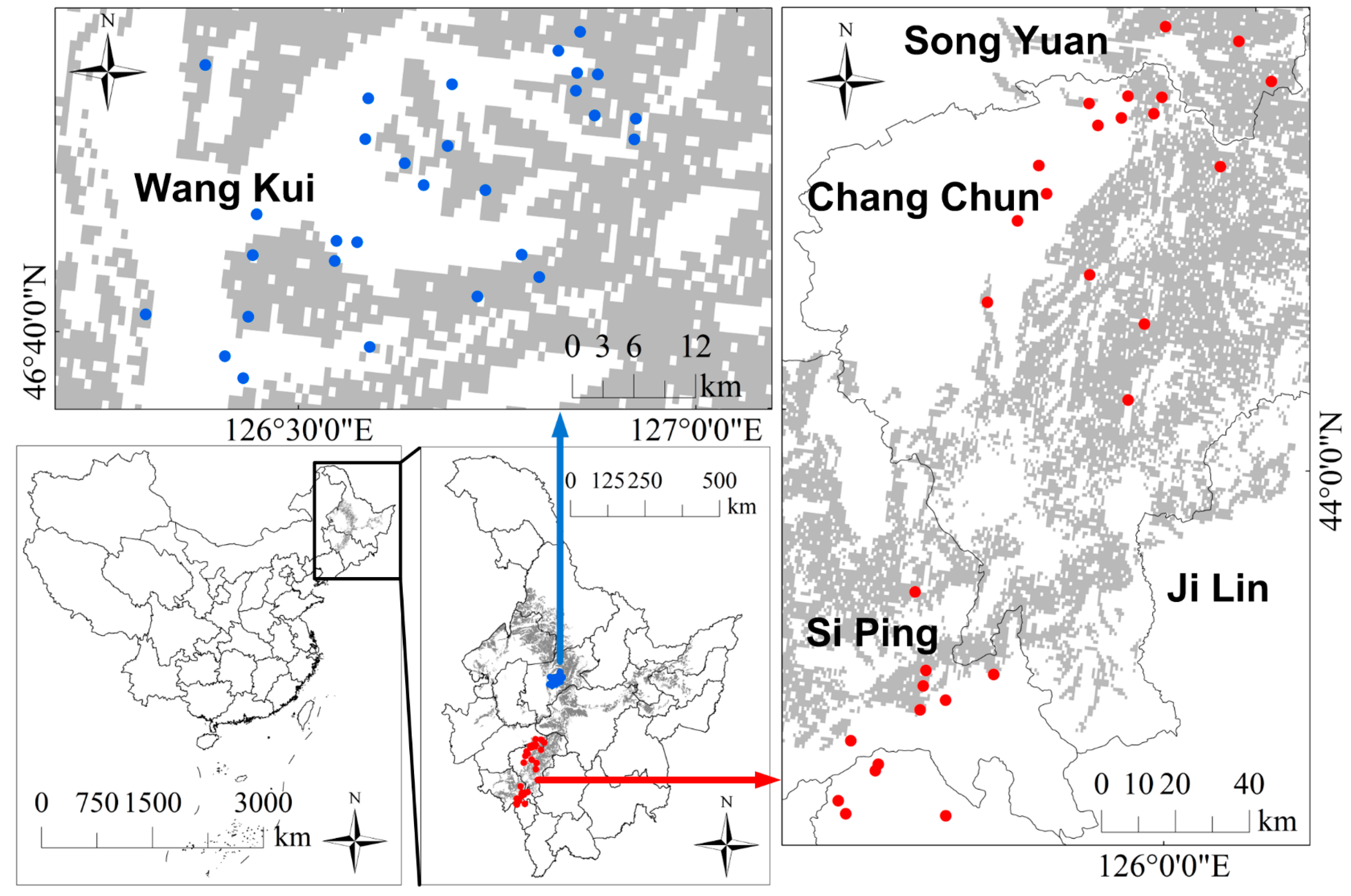
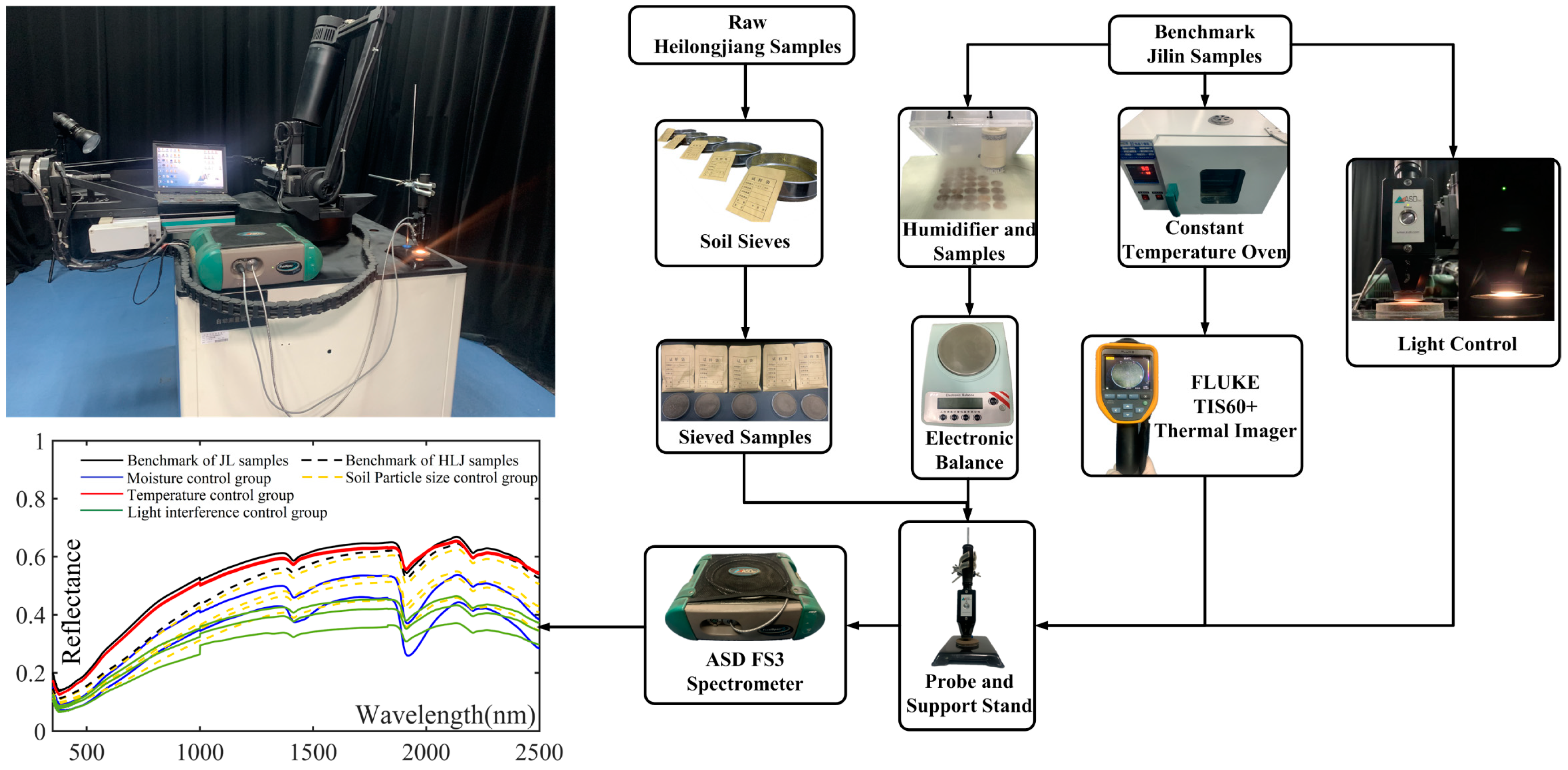
To this aim, we designed and performed four groups of control experiments in the standard spectral laboratory at Jilin University, China, to illustrate the spectral response under the influence of four independent variables: light interference, soil temperature, soil moisture, and soil particle size. Moreover, we chose the soil organic carbon (SOC) content, which is an important property of soil, as an indicator when performing the partial least squares regression (PLSR) calibration–validation to show the estimation ability of the spectra obtained from different groups of control experiments. Moreover, our study also considered employing spectral transformations, which have been applied in previous studies [31,32,33,34,35,36,37], for PLSR calibration–validation to provide conclusions that could be employed in future comparisons.

2. Materials and Methods

2.1. Basic Materials

2.1.1. Sampling Sites

Thirty soil samples collected from the typical black soil-covered (Haplic Phaenozems) [38] farmlands in Jilin province (124°55′5.71″E to 126°04′51.21″E, 43°03′5.04″N to 45°01′45.47″N) in October 2018 were used to perform light interference, soil temperature, and soil moisture control experiments (Figure 1 red points). Additionally, 30 soil samples for the soil particle size control experiment were collected in the typical black-soil-covered farmlands in Wangkui County, Heilongjiang province (42°33′19.51″N to 45°11′4.82″N, 124°55′45.07″E to 126°8’47.57″E) in July 2017 (Figure 1 blue points). At each sampling point, 2–3 kg of topsoil sample (0–20 cm) was collected for further spectral and geochemical testing, and each sampling point was recorded with WGS84 coordinates.

2.1.2. Soil Samples Pretreatment

Our Jilin (JL) soil samples were already processed in a course of air drying, crushing, and sieving through a 0.075 mm sieve and a soil organic carbon test. An analysis of soil organic carbon (SOC) content was carried out in the laboratory with the potassium dichromate volumetric method [39]. We fortunately obtained the other 30 Heilongjiang (HLJ) soil samples from Jilin Jianzhu University. These samples had not been finely sieved and retained field characteristics, which allowed us to design the control group with the single variable of soil particle size. Descriptions of the two datasets are listed in Table 1.

2.1.3. Basic Laboratory Materials

All soil samples were processed and spectrally measured in a standard spectral laboratory in Jilin University (JLU), China, which has constant laboratory environment and devices to support the control experiments: The darkroom was lined with a light-absorbing solid black cloth background; it contained a constant-temperature oven to control the temperature of the soil sample; a humidifier (mist maker) to adjust soil moisture; standard diameter metal mesh soil sieves; a thermal imager; high-precision electronic balance; support stand; Petri dishes, etc. The laboratory conditions and experimental materials are shown in Figure 2. An ASD Fieldspec® 3 high-resolution spectrometer with a high-intensity contact probe was used for soil sample spectral reflectance measurement. This spectrometer had the following characteristics: a spectral region of 350–2500 nm; a spectral resolution of 3 nm at the visible spectral region, 8.5 nm at the near-infrared, and 6.5 nm at the shortwave infrared spectral region; a 1 nm spectra sampling interval.

2.2. Sample Treatment and Control Experiments

A single-variable control method was used to perform the experiments in this study. Figure 2 shows the flowchart of this procedure. Experiments were performed in a constant-temperature environment (20 °C). The 0.075 mm-sieved JL samples and the HLJ samples were all oven-dried at 50 °C for 24 h and placed in the constant-temperature lab for cooling to room temperature; they were spectrally measured as benchmarks. During the spectral measurement course, the spectrometer and probe were warmed up for 60 min, the spectrometer was calibrated by white reference measuring standard per 10 min, and the soil sample was placed in a Petri dish and its surface was flattened for probe-contacted measuring five times for each experiment (except for the light interference control experiment). Based on these benchmarks, we, respectively, controlled the light interference, soil temperature, soil moisture, and the soil particle size as the single variables to design the four control groups to investigate the spectral reflectance response and the SOC estimation difference under their influence.

2.2.1. Light Interference Control Group

The first experiment was performed to control the light interference in the spectral measurement process. We fixed the probe on a support stand. The distances between the top of the probe and the surface of the soil sample in the Petri dish were set at 0.3 and 1 cm. Under each condition, the standard spectral measurement process (darkroom) was performed on the 30 Jilin samples to determine whether the probe–sample distance would disturb the spectra results (Figure 3b,c). Moreover, the spectral measurement at the 0.3 cm gap was replicated in an illuminated room condition to investigate the spectra variation under the interference of the light noise (Figure 3a).

2.2.2. Soil Temperature Control Group

In the second control experiment, the soil temperature was set as the single variable to detect its influence on the spectral reflectance and subsequent estimation accuracy. Each of the JL samples in Petri dishes were put in the constant-temperature (50 °C) oven for 10 min, heated successively, and then removed for surface temperature measurement. The surface temperature of each sample was recorded with a FLUKE TiS60 thermal imager (Figure 4). Furthermore, the spectral reflectance of each sample at 50 (usually lower), 40, and 30 °C was measured to analyze the variation in the spectra and their capacity for SOC content estimation modeling, comparing them with the results of the benchmark (20 °C). It should be explained that in order to protect and recover the soil samples, we set the heating temperature to no higher than 50 °C; what is more, the temperature of the soil samples removed from the oven for next spectral measurement were usually lower than 50 °C because they cooled down quickly in the low-room-temperature environment.

2.2.3. Soil Moisture Control Group

The third control experiment set the soil moisture as the single variable. The humidifier (mist maker) was infused with distilled water and put into a transparent box to create a wet space. All JL samples in Petri dishes were placed in the box and humidified for 5 min to simulate slightly wet conditions (Figure 5). The masses of all samples were recorded by the balance before and after humidification to determine the change in soil moisture. The steps were replicated for another 25 min of humidification to simulate severely wet conditions. Samples were spectrally measured simultaneously to determine the difference in obtained spectra and their capacity for SOC content estimation compared with the results of the benchmark.

2.2.4. Soil Particle Size Control Group

The raw Heilongjiang samples we obtained from Jilin Jianzhu University were already sieved through the 1 mm standard soil sieve. These soil samples were further sieved through 0.5, 0.25, 0.1, and 0.075 mm sieves to derive the 5 groups of samples for the spectral measurement. Figure 6 shows an example of the sieved soil samples. We observed that the sample sieved through the 1 mm sieve retained many impurities. The number and the size of impurities decreased with the reduction in mesh size. Impurities were visually imperceptible after sieving through a mesh size below 0.1 mm (Figure 6d). The spectral measurements of the 5 groups of samples were performed using the standard process, and the obtained spectra were applied in the investigation of the spectra difference and their capacity for SOC content estimation modeling.

2.3. Methodology

2.3.1. Spectra Pre-Processing

The spectra recorded by the spectrometer were smoothing processed using the Savitzky–Golay algorithm [40] and exported into ASCII by ViewSpec Pro software. The average of the 5 replicated measurements of each sample was calculated to represent its spectral reflectance (R). Studies usually carry out the spectral transformation procedure to enhance the spectral characteristics for improving the quantitative estimation accuracy in calibration–validation modeling [31,32,33,34,35,36,37]. This study employed three often-used forms, the first derivative of the reflectance (R’), the absorbance (A) [32], and the continuum removal (C) [41], to perform the spectral transformation. The original spectral reflectance and the results of the three forms of spectral transformation of the samples were considered in SOC estimation modeling. Overall, based on the design of the control experiments with different sample treatments, a total of 56 PLSR models were developed with different groups of spectra for comparative analysis (Table 2).

2.3.2. Partial Least Squares Calibration and Validation

Partial least squares regression (PLSR) was employed for calibration–validation modeling for SOC content estimation. The PLSR procedure has been demonstrated to be the most robust modeling method in solving high-dimensional collinear independent hyperspectral data modeling for soil properties, especially for SOC content estimation [5,42,43,44,45]. For the computations, we employed the SIMPLS algorithm in MATLAB (MathWorks, Inc. USA), which constructs the original independent variables (spectra) into orthogonal PLS components (also known as the latent variables) that represent linear combinations of them and further relates the dependent variables with the new PLS components by linear regression [46]. The number of the PLS components used in modeling is commonly determined by maximizing the percentage of variance explained in variables (PCTVAR) by the PLS components or minimizing the root mean square error (RMSE) in n-fold validation [36]. In this study, we defined an index, the normalized ratio of PCTVAR and RMSE (NRPR), in a 10-fold cross validation to determine the optimum number of PLS components for calibration by maximizing it. The RMSE values of estimation in calibration (RMSEc) and in 10-fold validation (RMSEv), as well as the coefficients of determination in calibration and validation (R2c and R2v), were employed to quantify the accuracy of estimation in this study.

3. Results

3.1. The PLSR Modeling Benchmarks

The normalized ratios of PCTVAR and RMSE (NRPR) of the PLS models that were developed with the spectral reflectance of Jilin (JL) and Heilongjiang (HLJ) benchmarks and their three forms of spectral transformation (R’, A, and C) are shown in Figure 7. The maximum NRPR indicates the optimum number of PLS components (PCs) for modeling. The subsequent PLS models developed with corresponding spectra derived from different control experiments should refer to the benchmarks to keep the PCs consistent.

3.2. Spectral Response and Estimation Results under Light Interference

The average spectral reflectance and corresponding three forms of spectral transformation of the JL samples in different light interference control experiments are presented in Figure 8a–d (the corresponding results of all samples are shown in Supplementary Figures S1–S4). It is seen in Figure 8a that from the benchmark to the darkroom 1 cm gap condition, the spectral reflectances had similar spectral shapes yet showed a generally reduced whole VNIR-SWIR spectral region. Benchmark spectra were apparently higher than other three treatments, no matter whether just considering the average or all cases. Figure 8c illustrates that the variation tendency of spectral absorbance was almost symmetric about the x-axis with the corresponding spectral reflectance. The spectral variations were not noticeably different in R’ and C spectral forms, yet it was easily distinguished in Figure 8a,c,d that the spectral discontinuity at the 1000 nm internal detector splice [9] was obviously magnified in light-intervening conditions.
SOC content estimation accuracy rates using PLSR based on the spectra of different light interference control groups with different spectral forms are listed in Table 3 (the corresponding scatterplots of the estimation results are shown in Supplementary Figure S5). Regarding the estimation accuracy of different forms of spectra, although the calibration accuracy was enhanced perfectly (R2c = 0.994) when applying the R’ spectra, the validation accuracy was relatively poor (R2v = 0.518). The models developed with the C spectra reached the lowest levels of both calibration and validation accuracies. In contrast, the models developed with the original spectral reflectance and spectral absorbance reached ideal validation accuracies (R2v = 0.873 and R2v = 0.720, respectively). As far as the controlled light interference was concerned, the three groups of control experiments reached lower R2v and higher RMSEv in most statistics. The 1 cm darkroom measured spectra showed the lowest estimation accuracies, no matter what form of spectral transformation was employed, which demonstrated that the illumination of the halogen bulb on the soil sample was severely weakened when the contact measuring was not performed [15]; subsequently, the derived spectral reflectance and certain subsequent estimation results were obviously influenced. The 0.3 cm darkroom and 0.3 cm illuminated measured spectra showed comparable validation accuracies that were slightly lower than the benchmarks.

3.3. Spectral Response and Estimation Results under Soil Temperature Interference

The average spectral reflectance and corresponding three forms of spectral transformation of the JL samples under different soil temperature control experiments are presented in Figure 9a–d (the corresponding results of all samples are shown in Supplementary Figures S6–S9). In most cases (Figure 9a,c, Figures S6 and S8), the higher temperature samples showed lower spectral reflectance (or higher absorbance), yet this variation was not noticeable. The average reflectance of samples at 30, 40 and 50 °C did not show a noticeable difference. The difference in spectra between the higher temperature samples and the benchmark was narrowed by R’ spectral transformation (Figure 9b). However, the variation in the absorption region in the ranges 350–560, 1360–1540, and 1820–2140 nm was obviously distinguished by continuum removal (Figure 9d).
Table 4 provides the estimation accuracies of PLSR models based on the spectra of different soil temperature control groups with different spectral forms (the corresponding scatterplots of estimation results are shown in Supplementary Figure S10). The original spectral reflectance provided the best validation accuracies. Although the accuracies were lower than the R results, the models developed with A spectra also presented acceptable results. The validation accuracies of models based on R’ and C spectra were relatively poor, which is consistent with previous studies reporting that, although the spectral transformation of the first derivative and the continuum removal of spectral reflectance could effectively enhance the calibration accuracies of statistical models [31,32,33,34,35,36,37], the characteristic spectral bands of certain specific soil attributes show obvious discontinuous and unstable variation on the whole VNIR-SWIR spectral region when the R’ and C spectra are employed, which can distinctly influence validation accuracies [47]. Regarding the influence of soil temperature on the spectra variation and corresponding estimation ability, the results showed no distinct regularities between the estimation accuracy and the variation in soil temperature: In most cases, the benchmark models developed with soil spectra measured at a soil temperature of 20 °C showed the best estimation accuracies; however, the model TaR’ (30 °C) obtained the highest R2v = 0.538 of the treatments in its group (Table 4 green zone). Moreover, the model TcR (50 °C) obtained the highest R2c = 0.947 of the models developed with spectral reflectance, even higher than the benchmark model (JLBR) (Table 4 red zone). In conclusion, the results showed that, although the variation of soil temperature had an effect on the estimation accuracy, the effect was slight and not certainly averse.

3.4. Spectral Response and Estimation Results under Soil Moisture Interference

We illustrated the mass change of all humidified JL samples to demonstrate their moisture change instead of calculating the water contents because the humidifying method in our experiment cannot always completely and evenly humidify the soil samples in a relatively short time. Therefore, using the calculated water content to represent the soil moisture change would not yield accurate results. As shown in Figure 10, the benchmark samples obtained an average mass gain of 1.644 g after 5 min of humidification, which was regarded as a slightly wet condition. Furthermore, soil samples had an average mass gain of 2.546 g after another 25 min of humidification, which was regarded as a severely wet condition.
The average spectral reflectance and corresponding three forms of spectral transformations of JL samples in different soil moisture control experiments are presented in Figure 11a–d (the corresponding results of all samples are shown in Supplementary Figures S11–S14). Figure 11a and Figure S11 show a common decrease in spectral reflectance with increasing moisture content [21,22,48]. In contrast, the spectral absorbance showed a tendency to increase with the soil moisture increase (Figure 11c and Figure S11). Moreover, it can be seen that the water absorption range in the SWIR domain was enhanced with the increase in soil moisture in the results of R, A and C spectra (Figure 11a,c,d, Figures S11, S13 and S14) [49,50,51]. The variations were not distinguished in R’ spectra.
Table 5 provides estimation accuracies of PLSR models based on the spectra of different soil moisture control groups with different spectral forms (the corresponding scatterplots of estimation results are shown in Supplementary Figure S15). Models developed with original spectral reflectance and spectral absorbance showed the ideal estimation abilities with a higher R2 and a lower RMSE. The validation accuracies of models based on R’ and C spectra were relatively poor. Regarding the influence of soil moisture on the spectra variation and corresponding SOC estimation ability, two groups of control experiments showed a decline in R2 and increase in RMSE in most statistics with the increase in soil moisture.

3.5. Spectral Response and Estimation Results under Soil Particle Size Interference

The average spectral reflectance and corresponding three forms of spectral transformation of the HLJ samples under different treatments of soil particle size control experiment are presented in Figure 12a,d (the corresponding results of all samples are shown in Supplementary Figures S16–S19). Figure 12a indicates that, ranging from the 0.075 mm (benchmark) sieved treatment to the 1 mm sieved treatment, the spectral reflectance of soil samples shared a similar spectral shape yet showed a general reduction in the whole VNIR-SWIR spectral region; this tendency is shown for all samples in Figure S16. Furthermore, as shown in Figure S16, in most cases the 0.075 and 0.1 mm sieved samples presented spectral reflectance at nearly the same level. The spectral reflectance values of soil samples in the 0.25 and 0.5 mm sieved treatments were also close. The 1 mm sieved samples all presented low-level results. Figure 12c and Figure S17 demonstrate the symmetric results of the A spectra and the R spectra, which shared consistent variation tendencies. Moreover, it was hard to observe the spectral variation of different soil samples from different particle size treatments in R’ and C spectral forms. The variation in the particle size of soil samples also did not cause distinct variations in the absorption region in the ranges 1360–1540 and 1820–2140 nm in R’ and C spectra, which was not consistent with the results of the moisture and temperature control experiments; however, the absorption peaks vibrated noticeably in the 350–560 nm range, as shown in Figure S19.
SOC content estimation accuracy using PLSR based on the spectra of different soil particle size control groups with different spectral forms is listed in Table 6 (the corresponding scatterplots of estimation results are shown in Supplementary Figure S20). PLSR models developed with four forms of spectra all reached ideal calibration accuracies; however, the validation accuracies of the R’ and C models were relatively poor. As far as the controlled variables for soil particle size are concerned, three groups of control experiments reached lower R2v and higher RMSEv than the benchmarks in all statistics. Excepting special cases (R2v = 0.909 of model PdR and R2v = 0.386 of model PdC were higher than the other three controlled cases), the validation accuracies of the models had a decreasing tendency with the increase in the particle size.

3.6. Observation of the Temperature of the Spectrometer and Probe

Considering that the soil temperature control experiment did not find a distinct correlation between the soil temperature and the corresponding estimation results, on the basis of the original experiment, we further monitored the temperature change of the spectrometer and the bulb under working conditions to determine the reason for the instability of the results.
As shown in Figure 13a, we directly measured the temperature of the bulb with the thermal imager during its working period. Because of the instrument body enclosure, it was difficult to directly obtain the working temperature of the spectrometer; hence, we recorded the temperature of the air outlet of the spectrometer as a representative value. We recorded the temperature with a one-minute interval from the start to stop of the device until it cooled to room temperature. As shown in Figure 13b, the temperature of the probe bulb sharply increased in the first minute, experienced a relatively slow increase from the 2nd to 24th minute, and then stabilized at around 50 °C. Meanwhile, the temperature of the spectrometer increased relatively rapidly up to about 26 °C before the 6th minute, experienced a sluggish increase from the 7th to 30th minute, and then stabilized at around 28 °C. We shut down the spectrometer at the 40th minute. We noted that the temperature of the bulb fell sharply to 34.5 °C in 2 min, cooled to 28.2 °C after 7 min, then experienced a long, sluggish cooling-down time to room temperature. Meanwhile, the temperature of the spectrometer experienced a stable decrease in about 20 min to room temperature.

4. Discussions

First, as a well-accepted method of soil spectral measurement in most laboratories over the world [15], measurements with a high-intensity contact probe usually require close probe–soil contact conditions [6,8,10,15]. This was consistent with the results of our study, where the close contact measurement indeed obtained the optimum estimation accuracy in validation (Table 3 and 
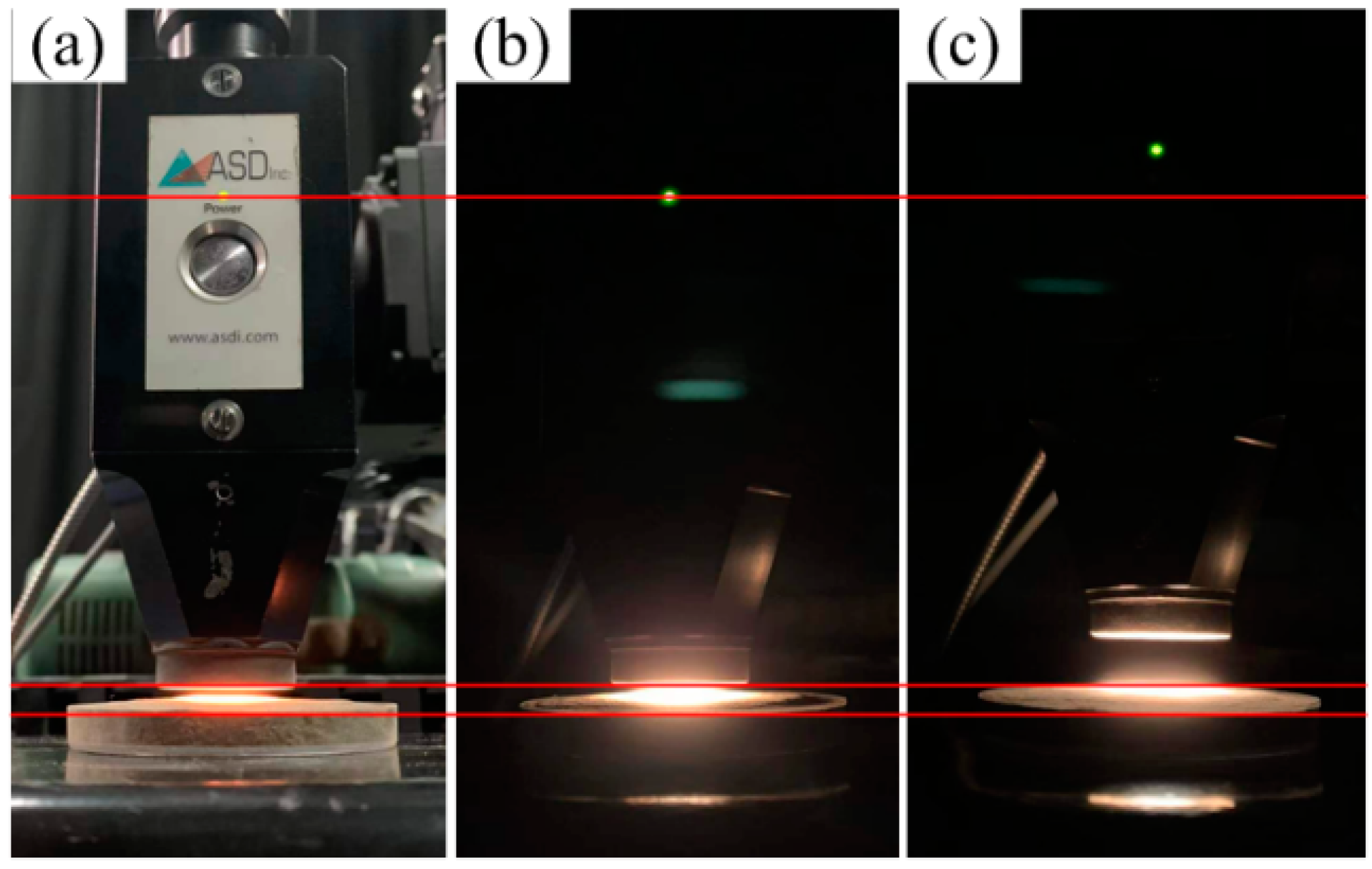
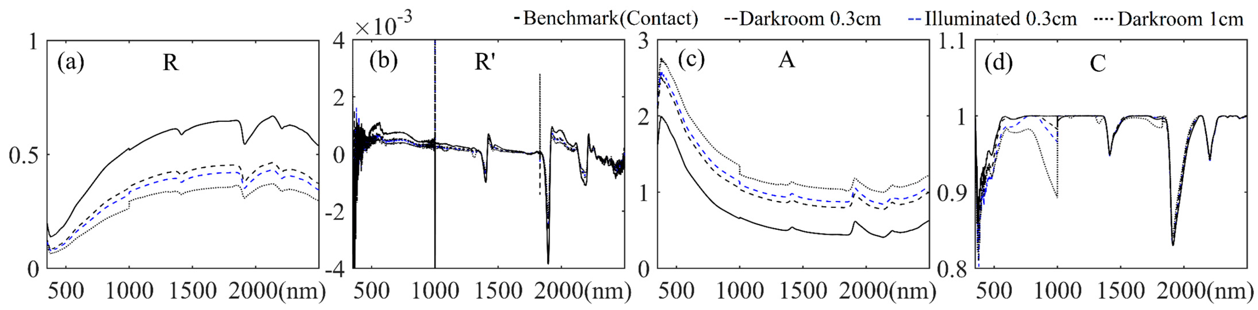
Figure S5). However, the different laboratory conditions and the special requirements of different operators (e.g., some laboratories prohibit the probe coming into contact with soil samples to avoid cross-contamination between samples and instruments) introduced the possibility of light interference in the measuring course. Correspondingly, our study presented a theoretical response to this problem by demonstrating that the close-non-contact measurement could also obtain a relatively lower but acceptable accuracy, even if under the illuminating interference environment. We also demonstrated that the large gap non-contact measurement could lead to a serious reduction in the spectra quality as well as the estimation accuracy. Hence, if there are no special requirements for experiments, we recommend using contact measurement to obtain the optimal spectra quality as far as possible.
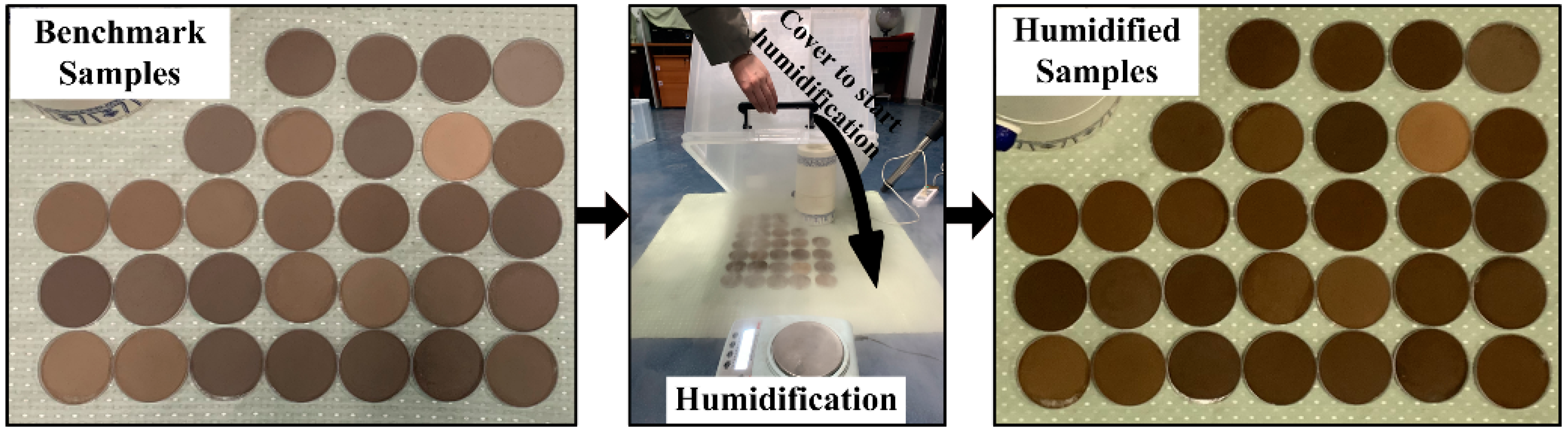
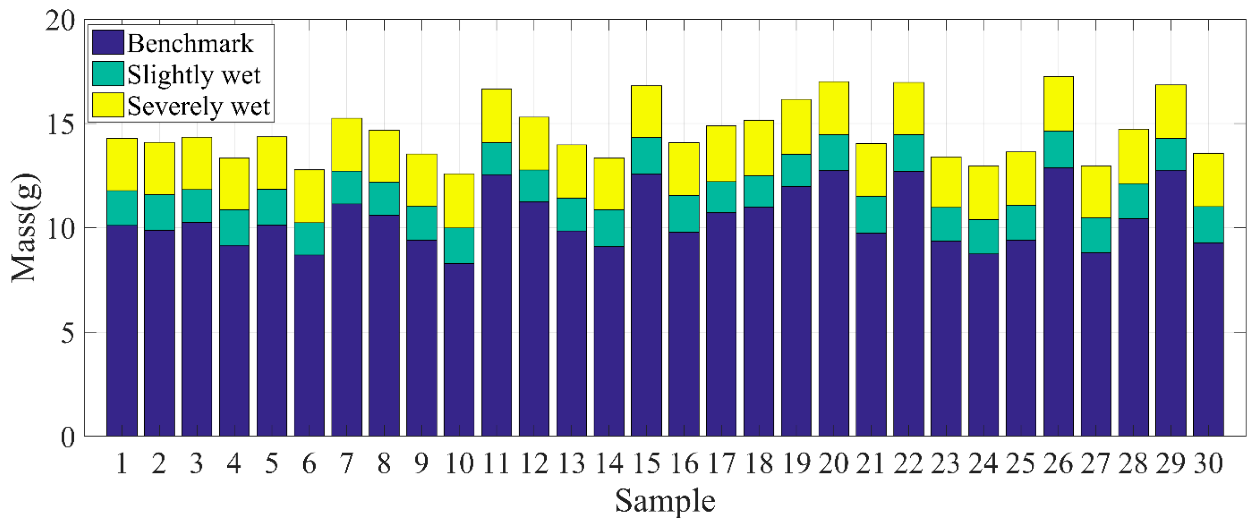
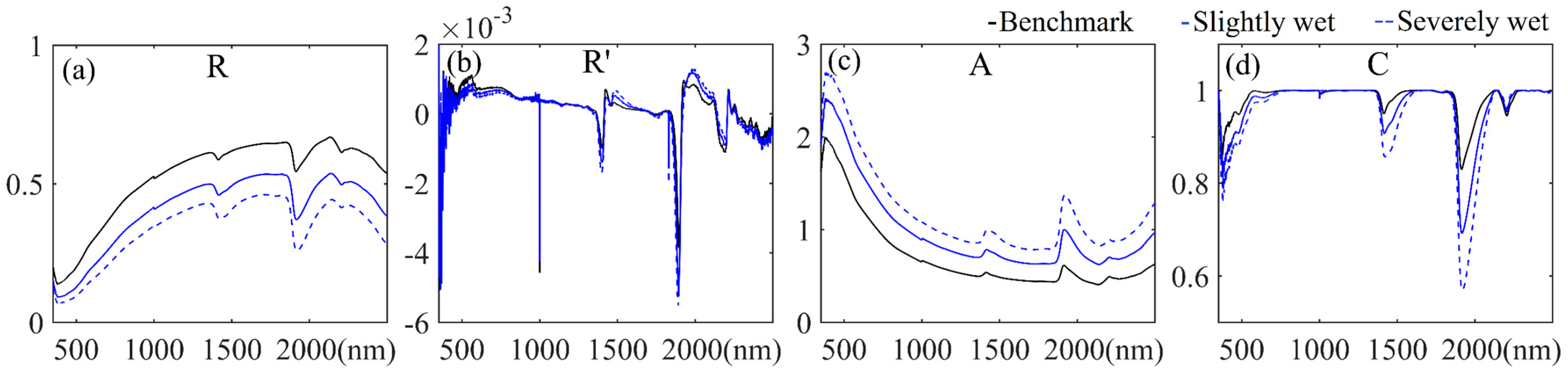
Second, the soil moisture control experiment demonstrated that soil moisture interferes the most significantly in the soil spectra quality of the four factors: The result showed a common decrease in spectral reflectance with increasing moisture content, which was consistent with previous studies [21,22,48]. Moreover, enhancement of the water absorption range in the SWIR domain with the increasing soil moisture [49,50,51] was distinctly detected in our experiment. The estimation accuracy significantly declined with the increase in soil moisture, which was consistent with most cases in previous studies [48,52]. Water in soil has been demonstrated to have a significant effect on the H2O expression spectral bands, which masks the major chemical chromophores in soils [3,53] and leads to unstable statistical characteristics of the modeling spectra. Moreover, this leads to poor accuracies in estimation results. Hence, we suggest that complete drying of soil samples is necessary in standard laboratory-based proximal spectral measurements.
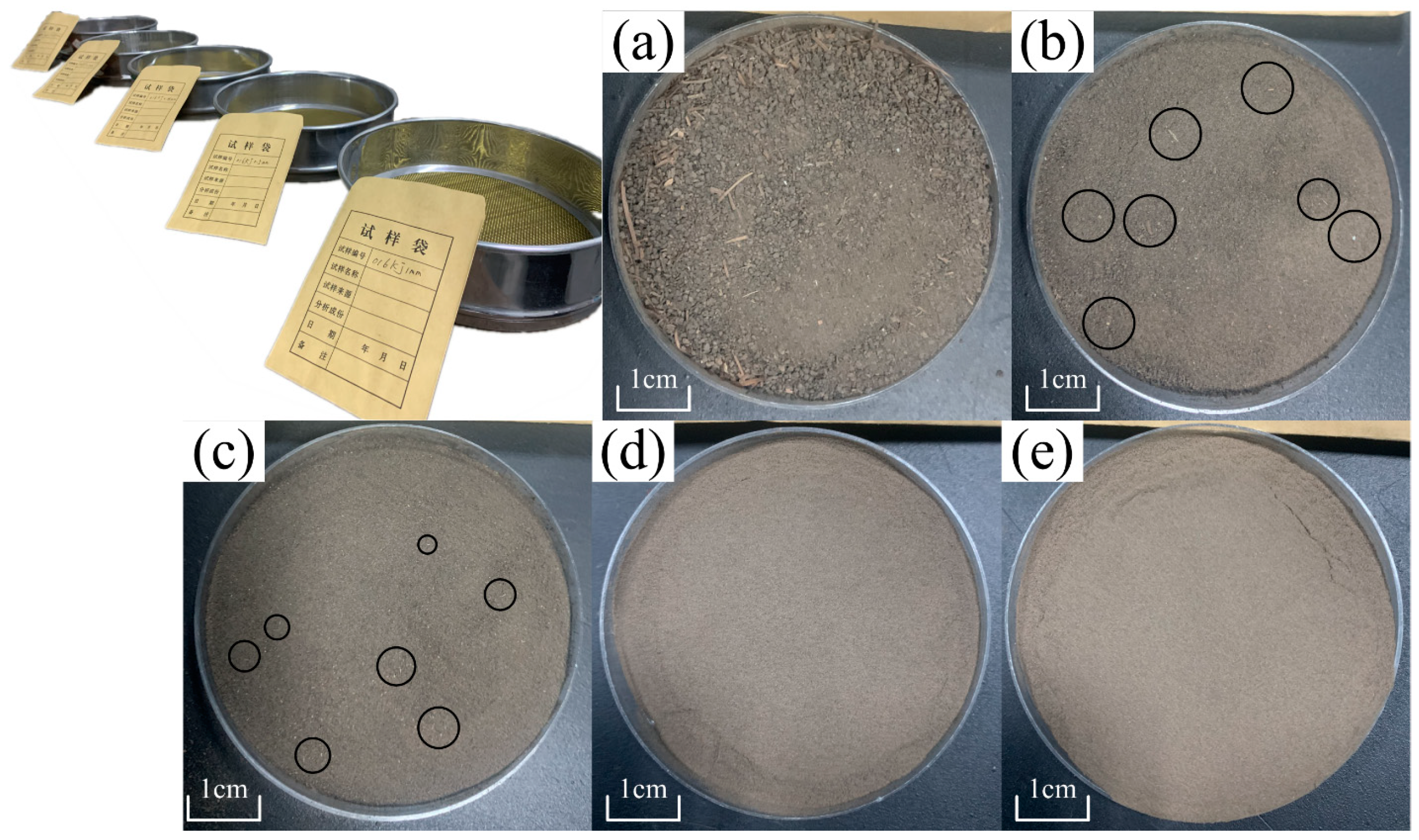
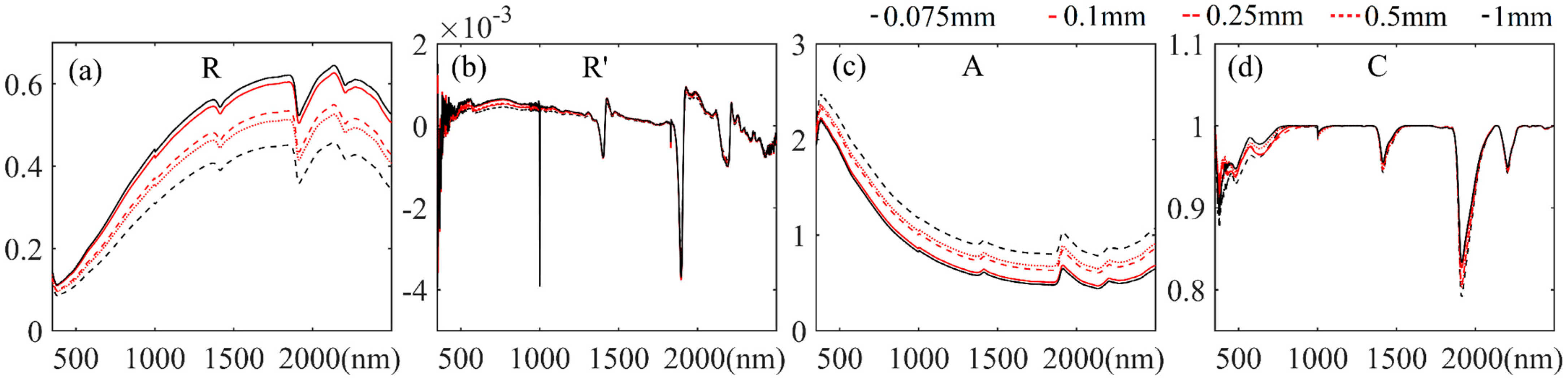
Third, the spectral reflectance of soil samples showed a general increase in the whole VNIR-SWIR spectral region with the decrease in soil particle size, a stable tendency observed in Figure 12 and Figure S16. Moreover, we demonstrated that the validation accuracies of the models were effectively enhanced by finely sieving, which was consistent with previous reports that indicated the transmission of light through soil samples would be affected and derived different spectral reflectance characteristics when the particle size changed, which can lead to significant variations in the estimation accuracies [54,55,56]. However, the optimum particle size suggested in previous reports differed (ranging from 0.88 to 2 mm) from our result [5,15,26,27,28]. One reason for this difference might be the effects of the different test methods used to obtain the modeling parameters. For instance, the laboratory methods for testing the SOC content are different, ranging from the dry combustion [9,16,18,56] to Walkley’s rapid method [54]. Different test methods require different soil particle sizes. For instance, this study employed the potassium dichromate volumetric method, which required the particle size of the employed soil sample to be less than 0.8 mm [39], which could explain why the particle sizes of soil samples that produced the optimum estimation accuracies were consistent with previous studies (less than 0.1 mm) employing the same methods [28,57]. In other words, the principles of existing modeling methods almost all depend on establishing the statistical relationship between the soil spectra and corresponding properties. Employing the same sieving level for geochemical tests and spectral measurement of the soil samples, in the meantime, helps to maintain the consistency of the target when establishing statistical relations. Hence, we suggest that preparing soil samples with a particle size under 1 mm can be accepted. Moreover, it is not necessary to require a particular unified sieving level in the development of a laboratory-based proximal spectral measurement protocol, but this should depend on different targets and methods.
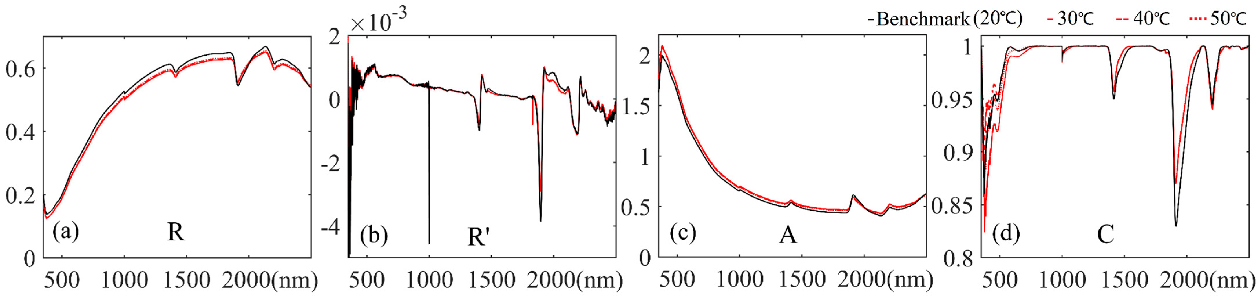
Last, the soil temperature control experiment did not establish a distinct correlation between the soil temperature and the corresponding estimation results. In most statistics, the estimation accuracy showed a lower R2 and a higher RMSE with the increase in soil temperature. However, this result was not obvious. We did not obtain consistent extension in the group of models developed with the spectral reflectance (R), in which the soil samples at 50 °C reached an even higher R2c with an ideal R2v than the other three controlled conditions (20, 30, and 40 °C) (Table 4 and Figure S10), as the previous study demonstrated [18]. According to the results of the additional experiment in our study (
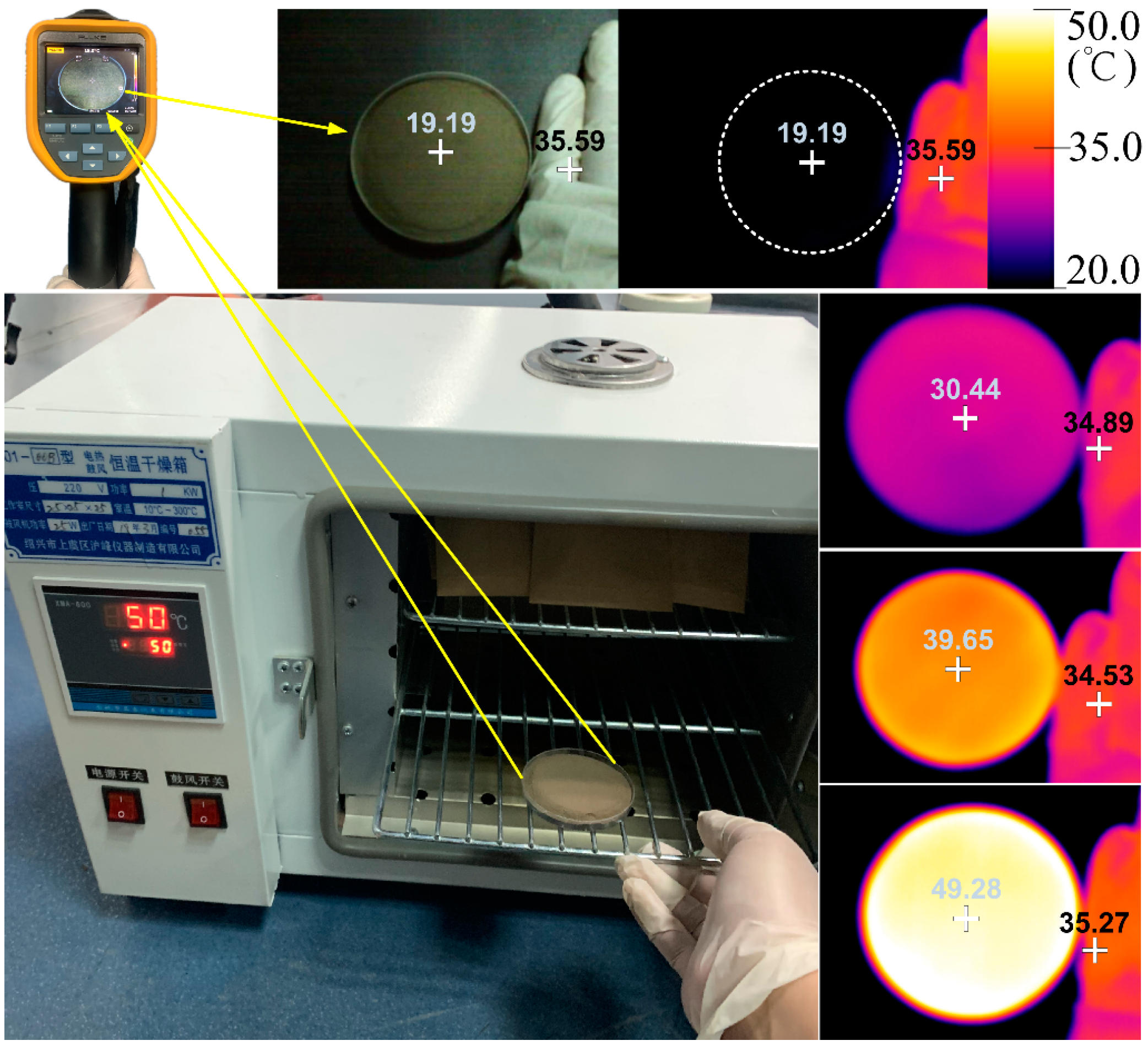
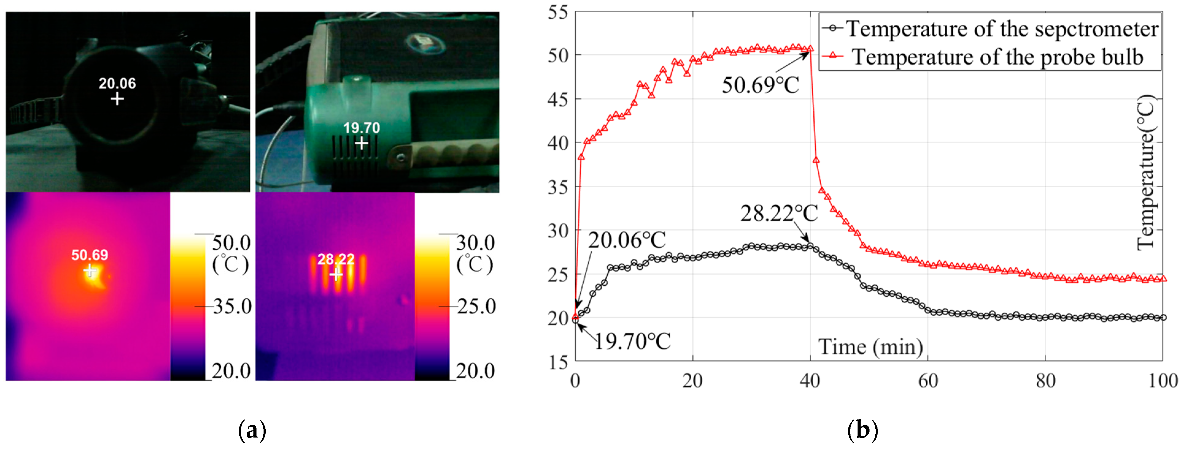
Section 3.6), we suppose that one factor causing the varying results might be the temperature disturbance by the contact probe. Figure 13b shows that the probe kept a 50 °C working temperature after 24 min of warming up. This means that even though the soil samples were processed to a uniform temperature for measurement, when the sample came into contact with the probe, the surface was heated by the 50 °C bulb, resulting in an uncontrollable temperature gain that might lead to the unstable variation in the obtained spectra. Overall, the estimation results did not demonstrate obvious regular variation with the change in the soil temperature; the estimation accuracies of the models developed with the spectral reflectance of soil samples under four temperature conditions (20–50 °C) were all acceptable (0.902 ≤ R2c ≤ 0.947; 0.798 ≤ R2v ≤ 0.873). Hence, we suggest that in order to ensure the efficiency of the spectral measurement procedure, the method of employing the room temperature samples for spectral measurement should continue to be popularized when developing standard laboratory protocol and future studies [10,11,15]. Moreover, the results of the additional experiment also demonstrated that the spectrometer and the contact probe bulb reached the stable working temperature in about 30 min, which also presents a guideline for specifying the warm-up time of the devices from the perspective of users.

5. Conclusions

For this study, we designed and performed control experiments to investigate the influence on the soil spectra quality and subsequent estimation accuracy of four key factors in a proximal spectral measurement procedure in a laboratory setting. Control experiments were performed in the standard spectral laboratory at Jilin University (JLU), China, which has a constant laboratory environment and devices needed to support the control experiments. Among the four key factors, light interference, soil moisture, and soil particle size demonstrated obvious influences on soil spectral characteristics and subsequent estimation accuracies. Furthermore, soil moisture interfered the most significantly in the soil spectra quality, with an evident decrease in spectral reflectance and significant decline in the estimation accuracy with increasing moisture content. However, the soil temperature control experiment did not obtain the ideal result and could not determine a distinct correlation between the soil temperature and the corresponding estimation results. From the results of the control experiments and comparative analysis, the conclusions presented below can be drawn to guide optimizing the process of laboratory-based proximal soil spectral measurements to derive a higher spectra quality and corresponding ideal estimation accuracies.
The soil–probe contact measurement derives the optimum spectra quality and estimation accuracy; however, close-non-contact measurement can also obtain a relatively lower but acceptable accuracy, even if under the illuminating interference environment. The complete drying procedure of soil samples is necessary in soil sample processing. Sieving below 1 mm particle size can produce soil samples with a high spectra quality and ideal estimation accuracy; moreover, specific sieving levels in further studies should be designed based on the different research objects and the referenced geochemical test methods. The method of employing the room temperature samples for spectral measurement can continue to be promoted in future studies; moreover, a 30-min warm-up time for the spectrometer and contact probe was demonstrated to be effective by the additional temperature observation experiment.
Despite carrying out this investigation and optimizing the four key factors in soil proximal spectral measurement, there is still room for further research to comprehensively investigate additional factors in the spectral measurement procedure that will influence the spectra quality and subsequent soil property estimation. Furthermore, as we mentioned in Section 3.4, the geochemical references are usually derived from different laboratory methods, and further comparative study to characterize their influence on the corresponding estimation accuracies can also promote the development of spectral measurement protocols. Moreover, although the reference factor used in this research, the SOC content, is an important soil property, the estimation results might be different when other soil properties are employed. Hence, the conclusions of this study must be confirmed by further detailed applications.

Supplementary Materials

Supplementary Materials are available online at https://www.mdpi.com/article/10.3390/rs14071558/s1, Text S1: Spectral response and estimation results of all JL samples under light interference (including Figures S1–S5); Text S2: Spectral response and estimation results of all JL samples under soil temperature influence (including Figures S6–S10); Text S3: Spectral response and estimation results of all JL samples under soil moisture influence (including Figures S11–S15); Text S4: Spectral response and estimation results of all HLJ samples under soil particle size influence (including Figures S16–S20).

Author Contributions

Conceptualization, Z.X. and S.C.; Methodology, Z.X.; Software, Z.X., Z.W., A.L. and L.C.; Validation, Z.X. and S.C.; Formal Analysis, Z.X.; Investigation, Z.X., Z.W. and Q.Z.; Resources, S.C. and P.L.; Data Curation, Z.X. and S.C.; Writing—Original Draft Preparation, Z.X.; Writing—Review and Editing, Z.X.; Visualization, Z.X.; Supervision, S.C.; Project Administration, S.C. and P.L.; Funding Acquisition, S.C. and P.L. All authors have read and agreed to the published version of the manuscript.

Funding

This research was supported by National Key Research and Development Program of China (No. 2020YFA0714103), Jilin Province Science and technology development plan (20210201138GX), Jilin Province Science and technology development plan (20210203016SF) and the Land Resource Evolution Mechanism and Its Sustainable Use in Global Black Soil Critical Zone (IGCP665) funded by IUGS and UNESCO.

Data Availability Statement

Due to confidentiality agreements, supporting data is not available in this study.

Acknowledgments

The HLJ soil samples and part of the experimental materials were provided by the College of Surveying and Exploration Engineering, Jilin Jianzhu University, Changchun, China. We would like to thank the researchers at the Heilongjiang Provincial Geology and Mineral Resources Test and Application Institute, China, as well as the laboratory in Liaoning Research Institute of Geology and Mineral Resources, China, who provided the materials and interpretation of the geochemical test methods.

Conflicts of Interest

We declare that we do not have any commercial or associative interest representing a conflict of interest in connection with the submitted manuscript.

References

  1. Bengera, I.; Norris, K.H. Determination of moisture content in soybeans by direct spectrophotometry. Isr. J. Agric. Res. 1968, 18, 124–132. [Google Scholar]
  2. Ben-Dor, E.; Banin, A. Visible and near-infrared (0.4–1.1 μm) analysis of arid and semiarid soils. Remote Sens. Environ. 1994, 48, 261–274. [Google Scholar] [CrossRef]
  3. Ben-Dor, E. Quantitative remote sensing of soil properties. Adv. Agron. 2002, 75, 173–243. [Google Scholar] [CrossRef]
  4. Pasquini, C. Near Infrared Spectroscopy: Fundamentals, practical aspects and analytical applications. J. Braz. Chem. Soc. 2003, 14, 198–219. [Google Scholar] [CrossRef] [Green Version]
  5. Viscarra Rossel, R.A.; Walvoort, D.J.J.; McBratney, A.B.; Janik, L.J.; Skjemstad, J.O. Visible, near infrared, mid infrared or combined diffuse reflectance spectroscopy for simultaneous assessment of various soil properties. Geoderma 2006, 131, 59–75. [Google Scholar] [CrossRef]
  6. Stenberg, B.; Viscarra-Rossel, R.A.; Mouazen, A.M.; Wetterlind, J. Visible and Near Infrared Spectroscopy in Soil Science. Adv. Agron. 2010, 107, 163–215. [Google Scholar] [CrossRef] [Green Version]
  7. Gholizadeh, A.; Boruvka, L. Common Chemometric Indicators for Prediction of Soil Organic Matter Content and Quality from Soil Spectra: A Review and Research Perspectives. In Proceedings of the International Workshop “Soil Spectroscopy: The Present and Future of Soil Monitoring”, Rome, Italy, 4 December 2013. [Google Scholar] [CrossRef]
  8. Chabrillat, S.; Ben-Dor, E.; Cierniewski, J.; Gomez, C.; Schmid, T.; Van Wesemael, B. Imaging Spectroscopy for Soil Mapping and Monitoring. Surv. Geophys. 2019, 40, 361–399. [Google Scholar] [CrossRef] [Green Version]
  9. Ge, Y.; Morgan, C.L.; Grunwald, S.; Brown, D.J.; Sarkhot, D.V. Comparison of soil reflectance spectra and calibration models obtained using multiple spectrometers. Geoderma 2011, 161, 202–211. [Google Scholar] [CrossRef]
  10. Kopačková, V.; Ben-Dor, E. Normalizing reflectance from different spectrometers and protocols with an internal soil standard. Int. J. Remote Sens. 2016, 37, 1276–1290. [Google Scholar] [CrossRef]
  11. Gholizadeh, A.; Carmon, N.; Klement, A.; Ben-Dor, E.; Borůvka, L. Agricultural Soil Spectral Response and Properties Assessment: Effects of Measurement Protocol and Data Mining Technique. Remote Sens. 2017, 9, 1078. [Google Scholar] [CrossRef] [Green Version]
  12. Chodak, M.; Ludwig, B.; Khanna, P.; Beese, F. Use of near infrared spectroscopy to determine biological and chemical char-acteristics of organic layers under spruce and beech stands. J. Plant Nutr. Soil Sci. 2002, 165, 27–33. [Google Scholar] [CrossRef]
  13. Udelhoven, T.; Emmerling, C.; Jarmer, T. Quantitative analysis of soil chemical properties with diffuse reflectance spectrometry and partial least-square regression: A feasibility study. Plant Soil 2003, 251, 319–329. [Google Scholar] [CrossRef]
  14. Brown, D.J. Using a global VNIR soil-spectral library for local soil characterization and landscape modeling in a 2nd-order Uganda watershed. Geoderma 2007, 140, 444–453. [Google Scholar] [CrossRef]
  15. Ben Dor, E.; Ong, C.; Lau, I.C. Reflectance measurements of soils in the laboratory: Standards and protocols. Geoderma 2015, 245, 112–124. [Google Scholar] [CrossRef]
  16. Reeves, J.; McCarty, G.; Mimmo, T. The potential of diffuse reflectance spectroscopy for the determination of carbon inventories in soils. Environ. Pollut. 2002, 116, S277–S284. [Google Scholar] [CrossRef]
  17. Nduwamungu, C.; Ziadi, N.; Parent, L.-É.; Tremblay, G.F.; Thuriès, L. Opportunities for, and limitations of, near infrared reflectance spectroscopy applications in soil analysis: A review. Can. J. Soil Sci. 2009, 89, 531–541. [Google Scholar] [CrossRef]
  18. Miltz, J.; Don, A. Optimising Sample Preparation and near Infrared Spectra Measurements of Soil Samples to Calibrate Organic Carbon and Total Nitrogen Content. J. Near Infrared Spectrosc. 2012, 20, 695–706. [Google Scholar] [CrossRef]
  19. Xiao, S.; He, Y. Application of Near-infrared Spectroscopy and Multiple Spectral Algorithms to Explore the Effect of Soil Particle Sizes on Soil Nitrogen Detection. Molecules 2019, 24, 2486. [Google Scholar] [CrossRef] [Green Version]
  20. Nie, P.; Dong, T.; He, Y.; Qu, F. Detection of Soil Nitrogen Using Near Infrared Sensors Based on Soil Pretreatment and Algorithms. Sensors 2017, 17, 1102. [Google Scholar] [CrossRef]
  21. Bowers, S.A.; Hanks, R.J. Reflection of radiant energy from soils. Soil Sci. 1965, 100, 130–138. [Google Scholar] [CrossRef] [Green Version]
  22. Neema, D.L.; Shah, A.; Patel, A.N. A statistical optical model for light reflection and penetration through sand. Int. J. Remote Sens. 1987, 8, 1209–1217. [Google Scholar] [CrossRef]
  23. Aurelien, B.; Vu, P.V.H.; Stéphane, J.; Françoise, V.; Sophie, F.; Xavier, B.; Morteza, S.; Michael, L.W.; Frédéric, B.; Jia, T. Marmit: A multilayer radiative transfer model of soil reflectance to estimate surface soil moisture content in the solar domain (400–2500 nm). Remote Sens. Environ. 2018, 217, 1–17. [Google Scholar]
  24. Waiser, T.H.; Morgan, C.L.S.; Brown, D.J.; Hallmark, C.T. In Situ Characterization of Soil Clay Content with Visible Near-Infrared Diffuse Reflectance Spectroscopy. Soil Sci. Soc. Am. J. 2007, 71, 389–396. [Google Scholar] [CrossRef]
  25. Fontán, J.M.; Calvache, S.; López-Bellido, R.J.; López-Bellido, L. Soil carbon measurement in clods and sieved samples in a Mediterranean Vertisol by Visible and Near-Infrared Reflectance Spectroscopy. Geoderma 2010, 156, 93–98. [Google Scholar] [CrossRef]
  26. Disla, J.S.; Janik, L.J.; Rossel, R.V.; Macdonald, L.; McLaughlin, M.J. The Performance of Visible, Near-, and Mid-Infrared Reflectance Spectroscopy for Prediction of Soil Physical, Chemical, and Biological Properties. Appl. Spectrosc. Rev. 2013, 49, 139–186. [Google Scholar] [CrossRef]
  27. Hou, Y.; Lv, C.; Xiang, H.; Wang, H. Treatment effects on soil hyperspectral stability in laboratory test. Chin. J. Soil Sci. 2013, 46, 287–291. (In Chinese) [Google Scholar]
  28. Wu, C.; Zheng, Y.; Yang, H.; Yang, Y.; Wu, Z. Effects of different particle sizes on the spectral prediction of soil organic matter. Catena 2020, 196, 104933. [Google Scholar] [CrossRef]
  29. Fearn, T. Standardisation and Calibration Transfer for near Infrared Instruments: A Review. J. Near Infrared Spectrosc. 2001, 9, 229–244. [Google Scholar] [CrossRef]
  30. Feudale, R.N.; Woody, N.A.; Tan, H.; Myles, A.J.; Brown, S.D.; Ferré, J. Transfer of multivariate calibration models: A review. Chemom. Intell. Lab. Syst. 2002, 64, 181–192. [Google Scholar] [CrossRef]
  31. Liu, H.; Yu, W.; Zhang, X.; Ma, Q.; Zhou, H.; Jiang, Z. Study on the main influencing factors of black soil spectral characteristics. Spectrosc. Spectr. Anal. 2009, 29, 3019–3022. [Google Scholar] [CrossRef]
  32. Rinnan, Å.; van den Berg, F.; Engelsen, S.B. Review of the most common pre-processing techniques for near-infrared spectra. TrAC Trends Anal. Chem. 2009, 28, 1201–1222. [Google Scholar] [CrossRef]
  33. Gholizadeh, A.; Borůvka, L.; Saberioon, M.; Kozák, J.; Vašát, R.; Němeček, K. Comparing different data preprocessing methods for monitoring soil heavy metals based on soil spectral features. Soil Water Res. 2016, 10, 218–227. [Google Scholar] [CrossRef] [Green Version]
  34. Nawar, S.; Buddenbaum, H.; Hill, J.; Kozak, J.; Mouazen, A.M. Estimating the soil clay content and organic matter by means of different calibration methods of vis-NIR diffuse reflectance spectroscopy. Soil Tillage Res. 2016, 155, 510–522. [Google Scholar] [CrossRef] [Green Version]
  35. Dotto, A.C.; Dalmolin, R.S.D.; Caten, A.T.; Grunwald, S. A systematic study on the application of scatter-corrective and spectral-derivative preprocessing for multivariate prediction of soil organic carbon by Vis-NIR spectra. Geoderma 2018, 314, 262–274. [Google Scholar] [CrossRef]
  36. Vašát, R.; Kodešová, R.; Klement, A.; Borůvka, L. Simple but efficient signal pre-processing in soil organic carbon spectroscopic estimation. Geoderma 2017, 298, 46–53. [Google Scholar] [CrossRef]
  37. Soltani, I.; Fouad, Y.; Michot, D.; Bréger, P.; Dubois, R.; Cudennec, C. A near infrared index to assess effects of soil texture and organic carbon content on soil water content. Eur. J. Soil Sci. 2018, 70, 151–161. [Google Scholar] [CrossRef] [Green Version]
  38. Liu, X.; Burras, C.L.; Kravchenko, Y.; Duran, A.; Huffman, T.; Morras, H.; Studdert, G.A.; Zhang, X.; Cruse, R.M.; Yuan, X. Overview of Mollisols in the world: Distribution, land use and management. Can. J. Soil Sci. 2012, 92, 383–402. [Google Scholar] [CrossRef]
  39. DZ/T 0279. 27-2016: Analysis Methods for Regional Geochemical Sample-Part 27: Determination of Organic Carbon Contents by Potassium Dichromate Volumetric Method. Available online: http://www.doc88.com/p-7724868306719.html (accessed on 17 January 2022).
  40. Savitzky, A.; Golay, M.J.E. Smoothing and Differentiation of Data by Simplified Least Squares Procedures. Anal. Chem. 1964, 36, 1627–1639. [Google Scholar] [CrossRef]
  41. Clark, R.N.; Roush, T.L. Reflectance spectroscopy: Quantitative analysis techniques for remote sensing applications. J. Geophys. Res. Solid Earth 1984, 89, 6329–6340. [Google Scholar] [CrossRef]
  42. Wold, S.; Sjöström, M.; Eriksson, L. PLS-regression: A basic tool of chemometrics. Chemom. Intell. Lab. Syst. 2001, 58, 109–130. [Google Scholar] [CrossRef]
  43. Castaldi, F.; Palombo, A.; Santini, F.; Pascucci, S.; Pignatti, S.; Casa, R. Evaluation of the potential of the current and forthcoming multispectral and hyperspectral imagers to estimate soil texture and organic carbon. Remote Sens. Environ. 2016, 179, 54–65. [Google Scholar] [CrossRef]
  44. Vaudour, E.; Gomez, C.; Fouad, Y.; Lagacherie, P. Sentinel-2 image capacities to predict common topsoil properties of temperate and Mediterranean agroecosystems. Remote Sens. Environ. 2019, 223, 21–33. [Google Scholar] [CrossRef]
  45. Biney, J.K.M.; Blöcher, J.R.; Borůvka, L.; Vašát, R. Does the limited use of orthogonal signal correction pre-treatment approach to improve the prediction accuracy of soil organic carbon need attention? Geoderma 2021, 388, 114945. [Google Scholar] [CrossRef]
  46. De Jong, S. SIMPLS: An alternative approach to partial least squares regression. Chemom. Intell. Lab. Syst. 1993, 18, 251–263. [Google Scholar] [CrossRef]
  47. Xu, Z.; Chen, S.; Zhu, B.; Chen, L.; Ye, Y.; Lu, P. Evaluating the Capability of Satellite Hyperspectral Imager, the ZY1–02D, for Topsoil Nitrogen Content Estimation and Mapping of Farmlands in Black Soil Area, China. Remote Sens. 2022, 14, 1008. [Google Scholar] [CrossRef]
  48. Nocita, M.; Stevens, A.; Noon, C.; van Wesemael, B. Prediction of soil organic carbon for different levels of soil moisture using Vis-NIR spectroscopy. Geoderma 2013, 199, 37–42. [Google Scholar] [CrossRef]
  49. Curcio, J.A.; Petty, C.C. The Near Infrared Absorption Spectrum of Liquid Water. J. Opt. Soc. Am. 1951, 41, 302. [Google Scholar] [CrossRef]
  50. Stoner, E.R.; Baumgardner, M.F. Physiochemical, Site and Bidirectional Reflectance Factor Characteristics of Uniformly Moist Soils; Purdue University: West Lafayette, IN, USA, 1979. [Google Scholar]
  51. Bedidi, A.; Cervelle, B.; Madeira, J.; Pouget, M. Moisture effects on visible spectral characteristics of lateritic soils. Soil Sci. 1992, 153, 129–141. [Google Scholar] [CrossRef]
  52. Tekin, Y.; Tumsavas, Z.; Mouazen, A.M. Effect of Moisture Content on Prediction of Organic Carbon and pH Using Visible and Near-Infrared Spectroscopy. Soil Sci. Soc. Am. J. 2012, 76, 188–198. [Google Scholar] [CrossRef]
  53. Barthès, B.G.; Brunet, D.; Ferrer, H.; Chotte, J.-L.; Feller, C. Determination of Total Carbon and Nitrogen Content in a Range of Tropical Soils Using near Infrared Spectroscopy: Influence of Replication and Sample Grinding and Drying. J. Near Infrared Spectrosc. 2006, 14, 341–348. [Google Scholar] [CrossRef]
  54. Krishnan, P.; Alexander, J.D.; Butler, B.J.; Hummel, J.W. Reflectance Technique for Predicting Soil Organic Matter. Soil Sci. Soc. Am. J. 1980, 44, 1282–1285. [Google Scholar] [CrossRef]
  55. Dalal, R.C.; Henry, R.J. Simultaneous Determination of Moisture, Organic Carbon, and Total Nitrogen by Near Infrared Reflectance Spectrophotometry. Soil Sci. Soc. Am. J. 1986, 50, 120–123. [Google Scholar] [CrossRef]
  56. Chang, C.-W.; Laird, D.A.; Mausbach, M.J.; Hurburgh, C.R., Jr. Near-Infrared Reflectance Spectroscopy-Principal Components Regression Analyses of Soil Properties. Soil Sci. Soc. Am. J. 2001, 65, 480–490. [Google Scholar] [CrossRef] [Green Version]
  57. Li, D.; Chen, X.; Peng, Z.; Chen, S.; Chen, W.; Han, L.; Li, Y. Prediction of soil organic matter content in a litchi orchard of South China using spectral indices. Soil Tillage Res. 2012, 123, 78–86. [Google Scholar] [CrossRef]
Figure 1. The geographic extent of the sampling sites: dark background indicates the typical black soil area in northeast China. Blue and red points indicate sampling points in Heilongjiang and Jilin.
Remotesensing 14 01558 g001
Figure 2. The standard spectral laboratory in JLU: darkroom environment (top left), device interaction flow chart (right), and the average spectral reflectance of each control group (bottom left).
Remotesensing 14 01558 g002
Figure 3. (a) Probe setup with 0.3 cm gap in illuminated room condition; (b) probe setup with 0.3 cm gap in darkroom condition; (c) probe setup with 1 cm gap in darkroom condition; three red lines of reference indicate the position change of the probe.
Remotesensing 14 01558 g003
Figure 4. Sample heating and surface temperature recording. The surface temperature of the benchmark sample is represented as the visible light image (top left) and infrared image (top right). The heated samples are represented as infrared images on the right. The fingers of the researcher are depicted as references.
Remotesensing 14 01558 g004
Figure 5. The humidification box and samples.
Remotesensing 14 01558 g005
Figure 6. Standard diameter metal mesh soil sieves and sieved samples: (a) 1 mm sieved sample; (b) 0.5 mm sieved sample; (c) 0.25 mm sieved sample; (d) 0.1 mm sieved sample; and (e) 0.075 mm sieved sample.
Remotesensing 14 01558 g006
Figure 7. The NRPRs of different numbered PLS components (PCs) of eight benchmark models. As explained in detail in Table 2, the model names in Figure 7 correspond to: JLB: JL Benchmark; HB: HLJ Benchmark; R, R’, A and C in model names correspond to four forms of spectra.
Remotesensing 14 01558 g007
Figure 8. Average spectra of JL samples in light interference control experiments: (a) spectral reflectance (R); (b) the first derivative of the reflectance (R’); (c) the spectral absorbance (A); and (d) the spectra of continuum removal (C).
Remotesensing 14 01558 g008
Figure 9. Average spectra of JL samples in soil temperature control experiments: (a) spectral reflectance (R); (b) the first derivative of the reflectance (R’); (c) the spectral absorbance (A); (d) the spectra of continuum removal (C).
Remotesensing 14 01558 g009
Figure 10. The mass changes of all Jilin benchmark samples after 5 and 30 min of humidification.
Remotesensing 14 01558 g010
Figure 11. Average spectra of JL samples in soil moisture control experiments: (a) spectral reflectance (R); (b) the first derivative of the reflectance (R’); (c) the spectral absorbance (A); and (d) the spectra of continuum removal (C).
Remotesensing 14 01558 g011
Figure 12. Average spectra of HLJ samples in soil particle size control experiments: (a) spectral reflectance (R); (b) the first derivative of the reflectance (R’); (c) the spectral absorbance (A); (d) the spectra of continuum removal (C).
Remotesensing 14 01558 g012
Figure 13. (a) Temperature measurement of the spectrometer and the bulb in the probe; (b) temperature variation during the working period.
Remotesensing 14 01558 g013
Table 1. Soil datasets for this research.
DatasetsSOC Content (%)SDCV
MinQ1MedianQ3MaxMean
JL0.912.502.632.473.702.600.520.20
HLJ1.782.622.512.173.762.550.410.16
Q1: the first quartile; Q3: the third quartile; SD: standard deviation; CV: coefficient of variation.
Table 2. A list of the PLSR models developed with different sample sets under different treatments and four forms of spectral transformations.
Sample SetControl ExperimentTreatmentSpectra FormModel
JilinBenchmarkStandardR/R’/A/CModel JLBR/JLBR’/JLBA/JLBC
LightDarkroom 0.3 cmR/R’/A/CModel LaR/LaR’/LaA/LaC
Illuminated 0.3 cmR/R’/A/CModel LbR/LbR’/LbA/LbC
Darkroom 1 cmR/R’/A/CModel LcR/LcR’/LcA/LcC
Temperature30 °CR/R’/A/CModel TaR/TaR’/TaA/TaC
40 °CR/R’/A/CModel TbR/TbR’/TbA/TbC
50 °CR/R’/A/CModel TcR/TcR’/TcA/TcC
Moistureslightly wetR/R’/A/CModel MaR/MaR’/MaA/MaC
severely wetR/R’/A/CModel MbR/MbR’/MbA/MbC
HeilongjiangParticle size0.075 mm sievedR/R’/A/CModel HBR/HBR’/HBA/HBC
0.1 mm sievedR/R’/A/CModel PaR/PaR’/PaA/PaC
0.25 mm sievedR/R’/A/CModel PbR/PbR’/PbA/PbC
0.5 mm sievedR/R’/A/CModel PcR/PcR’/PcA/PcC
1 mm sievedR/R’/A/CModel PdR/PdR’/PdA/PdC
Table 3. Estimation accuracy of PLS models in the light interference control experiment.
ModelJLBRLaRLbRLcRJLBR’LaR’LbR’LcR’
R2c0.938 0.944 0.929 0.914 0.994 0.984 0.990 0.981
R2v0.873 0.852 0.823 0.789 0.518 0.156 0.276 −0.351
RMSEc0.128 0.122 0.137 0.150 0.041 0.065 0.050 0.071
RMSEv0.182 0.197 0.216 0.235 0.356 0.470 0.436 0.595
ModelJLBALaALbALcAJLBCLaCLbCLcC
R2c0.893 0.931 0.927 0.921 0.748 0.861 0.801 0.694
R2v0.720 0.665 0.656 0.650 0.285 0.130 0.200 −0.265
RMSEc0.167 0.135 0.139 0.144 0.257 0.191 0.229 0.283
RMSEv0.271 0.296 0.300 0.303 0.433 0.477 0.458 0.576
As explained in detail in Table 2, the model names in Table 3 correspond to: JLB: Jilin Benchmark (contact measurement); a, b, and c in model names refer to Darkroom 0.3 cm treatment, Illuminated 0.3 cm treatment, and Darkroom 1 cm treatment, respectively; R, R’, A, and C in model names refer to the four forms of spectra.
Table 4. Estimation accuracy of PLS models in the soil temperature control experiment.
ModelJLBRTaRTbRTcRJLBR’TaR’TbR’TcR’
R2c0.938 0.902 0.934 0.947 0.994 0.993 0.984 0.995
R2v0.873 0.798 0.867 0.857 0.518 0.538 0.296 0.344
RMSEc0.128 0.160 0.132 0.118 0.041 0.043 0.064 0.035
RMSEv0.182 0.230 0.187 0.194 0.356 0.347 0.430 0.415
ModelJLBATaATbATcAJLBCTaCTbCTcC
R2c0.893 0.854 0.875 0.885 0.748 0.719 0.921 0.896
R2v0.720 0.574 0.673 0.689 0.285 −0.500 0.100 −0.008
RMSEc0.167 0.196 0.181 0.174 0.257 0.272 0.144 0.166
RMSEv0.271 0.334 0.293 0.285 0.433 0.627 0.486 0.514
As explained in detail in Table 2, the model names in Table 4 correspond to: JLB: Jilin Benchmark (20 °C); a, b, and c in model names refer to 30, 40, and 50 °C, respectively; R, R’, A, and C in model names refer to four forms of spectra.
Table 5. Estimation accuracy of PLS models in the soil moisture control experiment.
ModelJLBRMaRMbRJLBR’MaR’MbR’JLBAMaAMbAJLBCMaCMbC
R2c0.938 0.884 0.857 0.994 0.973 0.990 0.893 0.880 0.865 0.748 0.603 0.730
R2v0.873 0.721 0.587 0.518 −0.293 0.180 0.720 0.621 0.533 0.285 −0.390 0.146
RMSEc0.128 0.175 0.194 0.041 0.085 0.051 0.167 0.178 0.188 0.257 0.322 0.266
RMSEv0.182 0.270 0.329 0.356 0.582 0.464 0.271 0.315 0.350 0.433 0.604 0.473
As explained in detail in Table 2, the model names in Table 5 correspond to: JLB: Jilin Benchmark (20 °C); a and b in model names refer to lightly wet and severely wet, respectively; R, R’, A, and C in model names refer to four forms of spectra.
Table 6. Estimation accuracy of PLS models in the soil particle size control experiment.
ModelHBRPaRPbRPcRPdRHBR’PaR’PbR’PcR’PdR’
R2c0.980 0.968 0.961 0.959 0.971 0.973 0.972 0.952 0.961 0.957
R2v0.919 0.876 0.853 0.850 0.909 0.603 0.702 0.347 0.279 0.231
RMSEc0.057 0.072 0.079 0.081 0.068 0.066 0.067 0.087 0.079 0.083
RMSEv0.114 0.141 0.153 0.155 0.120 0.252 0.218 0.323 0.339 0.350
ModelHBAPaAPbAPcAPdAHBCPaCPbCPcCPdC
R2c0.999 0.999 0.998 0.999 0.999 0.987 0.989 0.979 0.983 0.980
R2v0.925 0.801 0.758 0.741 0.743 0.431 0.312 0.300 0.296 0.386
RMSEc0.010 0.012 0.016 0.014 0.014 0.045 0.042 0.058 0.052 0.057
RMSEv0.109 0.179 0.197 0.203 0.202 0.301 0.331 0.334 0.335 0.313
As explained in detail in Table 2, the model names in Table 6 correspond to: JLB: Jilin Benchmark (0.075 mm particle size); a, b, c and d in model names refer to particle sizes of 0.1, 0.25, 0.5, and 1 mm, respectively; R, R’, A, and C in model names refer to the four forms of spectra.
Publisher’s Note: MDPI stays neutral with regard to jurisdictional claims in published maps and institutional affiliations.

