Article

Mapping Forest Aboveground Biomass Using Multisource Remotely Sensed Data

1
Department of Geography, University of North Carolina at Chapel Hill, Chapel Hill, NC 27599, USA
2
Department of Earth, Marine and Environment Sciences, University of North Carolina at Chapel Hill, Chapel Hill, NC 27599, USA
3
Eastern Forest Environmental Threat Assessment Center, USDA Forest Service, Raleigh, NC 27709, USA
4
Institute for a Secure and Sustainable Environment, University of Tennessee at Knoxville, Knoxville, TN 37996, USA
5
Carolina Population Center, University of North Carlina at Chapel Hill, Chapel Hill, NC 27599, USA
6
Department of Sociology, University of North Carolina at Chapel Hill, Chapel Hill, NC 27599, USA
7
Department of Earth and Environment, Boston University, Boston, MA 02215, USA
*
Author to whom correspondence should be addressed.
Remote Sens. 2022, 14(5), 1115; https://doi.org/10.3390/rs14051115
Submission received: 6 February 2022 / Revised: 19 February 2022 / Accepted: 22 February 2022 / Published: 24 February 2022
(This article belongs to the Special Issue Remote Sensing of Carbon Cycle Science)

Abstract

:
The majority of the aboveground biomass on the Earth’s land surface is stored in forests. Thus, forest biomass plays a critical role in the global carbon cycle. Yet accurate estimate of forest aboveground biomass (FAGB) remains elusive. This study proposed a new conceptual model to map FAGB using remotely sensed data from multiple sensors. The conceptual model, which provides guidance for selecting remotely sensed data, is based on the principle of estimating FAGB on the ground using allometry, which needs species, diameter at breast height (DBH), and tree height as inputs. Based on the conceptual model, we used multiseasonal Landsat images to provide information about species composition for the forests in the study area, LiDAR data for canopy height, and the image texture and image texture ratio at two spatial resolutions for tree crown size, which is related to DBH. Moreover, we added RaDAR data to provide canopy volume information to the model. All the data layers were fed to a Random Forest (RF) regression model. The study was carried out in eastern North Carolina. We used biomass from the USFS Forest Inventory and Analysis plots to train and test the model performance. The best model achieved an R2 of 0.625 with a root mean squared error (RMSE) of 18.8 Mg/ha (47.6%) with the “out-of-bag” samples at 30 × 30 m spatial resolution. The top five most important variables include the 95th, 85th, 75th, and 50th percentile heights of the LiDAR points and their standard deviations of 85th heights. Numerous features from multiseasonal Sentinel-1 C-Band SAR, multiseasonal Landsat 8 imagery along with image texture features from very high-resolution imagery were selected. But the importance of the height metrics dwarfed all other variables. More tests of the conceptual model in places with a broader range of biomass and more diverse species composition are needed to evaluate the importance of other input variables.

Graphical Abstract

1. Introduction

1.1. Importance of Forests in Global Carbon Cycle

Forests provide essential ecosystem goods and services upon which human welfare depends. Removing CO2 from the atmosphere through photosynthesis and storing the carbon as organic matter are among the most critical services forest ecosystems provide. CO2 in the atmosphere is the major greenhouse gas that causes global warming [1]. The current concentration of CO2 in the atmosphere is the highest in the past 800,000 years [2]. Since the Industrial Revolution, the extra CO2 released into the atmosphere has contributed to 2/3 of the extra energy that all greenhouse gases have trapped [3]. The majority of the increased CO2 in the atmosphere comes from fossil fuel burning, while land-use change, primarily deforestation, also contributed a significant amount of CO2 to the atmosphere [4,5]. Reducing emissions from deforestation and forest degradation, plus sustainable forest management, conservation, and enhancement of forest carbon stocks (REDD+), has been recognized as a major mechanism for global warming mitigation (http://un-redd.org, accessed on 5 February 2022). REDD+ projects are primarily implemented in developing countries in the tropical region, with funding donated from developed countries. However, deforestation and forest degradation can happen anywhere in the world as a result of both natural and anthropogenic disturbances. In contrast, forest growth could significantly offset the carbon emissions from fossil fuel burning. Removing CO2 from the atmosphere by forests is one of the most economically efficient nature-based solutions for global warming mitigation [6]. In fact, the vast majority of the Earth’s aboveground carbon is stored in forests as biomass. Therefore, forests play a critical role in the global carbon cycle. According to the most recent accounting, we still cannot balance the global carbon budget [7]. One of the critical limitations in balancing the global carbon budget is the lack of accurate information about forest biomass and its dynamics over time. Without accurate forest biomass information, we do not know the amount of carbohydrates produced in photosynthesis and accumulated through time in the forests. Consequently, we do not know how much carbon is released from the forest ecosystem due to natural and anthropogenic disturbances, such as deforestation from timber harvesting or shifting agriculture, wildfires, forest destruction from hurricanes, mass mortality from droughts [8,9,10] or insect infestations [11]. Therefore, knowledge about where forest biomass is located and how it is changing with time is vital for global carbon cycle science and, consequently, global climate change in the future.

1.2. Biomass Estimation on the Ground

Forest biomass is the total dry weight of all live parts of every tree in a unit area, including the parts both aboveground (leaves, branches, and stems) and belowground (fine and coarse roots) [12]. Forest Aboveground Biomass (FAGB) is the total forest biomass minus the belowground components, which have to be estimated through excavation [13]. FAGB is relatively easy to obtain and thus is often sought after instead of the total biomass that includes both above- and belowground components. The most reliable approach to estimate biomass on the ground is through destructive sampling, in which standard trees are cut, and their biomass is estimated from drying samples of the fresh components (e.g., leaves, branches, and stems). Then a species-specific allometric relationship of biomass is derived based on the tree height and diameter at breast height (DBH). The allometry is then applied to all the standing trees to estimate their biomass by species within a sampling plot. Summarizing the biomass from all trees within the sampling plot provides an area-based biomass estimation [12]. Tremendous efforts had been dedicated to developing the species-specific allometric relationships for forest biomass [14,15]. These allometric relationships can be re-used in the place where they were developed. Despite the availability of allometric equations for biomass for nearly all the major species in the U.S. and possibly most countries in the world, they cannot be directly used over large areas as we cannot obtain DBH, height, and species continuously in space for each tree. Although the existing allometric relationships for biomass cannot be used with remote sensing data, the variables used for estimating biomass with allometry should guide the selection of remotely sensed features for accurate biomass estimation, i.e., we need information related to species, DBH, and height to estimate forest biomass accurately over space and time. Many forest biomass products exist [16,17,18], but they are not produced based on such a principle. Consequently, accurate estimation of forest biomass over large areas remains elusive [19].

1.3. Challenges in Estimating Forest Aboveground Biomass with Remote Sensing

Remotely sensed data from nearly all types of sensors have been used to estimate FAGB because remotely sensed data can be used to derive a biomass surface. Optical remotely sensed data can be used to effectively estimate the gross primary production of the terrestrial ecosystem [20,21,22]. Gross primary production is the total carbon flux from the atmosphere to the terrestrial ecosystem through photosynthesis. A large portion of gross primary production is consumed by vegetation via autotrophic respiration [23]. The balance of gross primary production after autotrophic respiration is the net primary production, which shows up in plant growth. Not all the net primary production is accumulated through time due to litterfall and mortality [24]. Disturbances from both natural and anthropogenic origins also significantly alter FAGB almost instantaneously. Thus, the dynamics of FAGB are jointly controlled by forest growth and disturbances [25]. Forest biomass dynamics through time are critical information for future global carbon cycle prediction.
Nearly all the optical remotely sensed data currently available had been used for biomass mapping [19]. Spectral reflectance, transformed spectral reflectance (e.g., principal components, Tasseled Cap components, and vegetation indices), and the spatial information (e.g., image texture) have been used as independent variables for biomass estimation [26]. Song [12] identified three primary approaches used to estimate biomass from optical images, including k-nearest neighbor imputation, multiple regression, and machine learning algorithms. More recently, Pflugmacher et al. [27], took advantage of the long-term record of Landsat imagery and developed an algorithm to map FAGB using disturbance and recovery history.
Although tremendous efforts have been dedicated to mapping FAGB with remotely sensed data, the margin of error remains too big to help close the global carbon budget gap. The major challenge in mapping FAGB is that there is no direct remotely sensed biomass signal, unlike the leaf area index. We can only estimate biomass through remotely sensed signals that are correlated to biomass. For example, the leaf area index was used to estimate biomass [28]. However, these signals only work when the biomass is low. Forest leaf area index reaches its asymptote early in its successional stage [29], while the biomass of a forest continues to increase for centuries [30]. Remotely sensed signals that are correlated to forest aboveground biomass, such as vegetation indices or surface reflectance in a particular wavelength, saturate when biomass reaches a threshold of 100–200 mg/ha. Signal saturation from optical and RaDAR sensors is the primary reason why remote sensing-based approaches mapping FAGB do not work well when the FAGB is beyond that threshold from these sensors [19,31,32,33].
Similarly, extensive research had been conducted on mapping FAGB with RaDAR data, recently reviewed by [19]. There are consistent findings that the backscatter intensity from the longer wavelength (L- or P-band) is better correlated with FAGB than that from the shorter wavelength (C-band) because the longer wavelength RaDAR waves penetrate deeper into the canopy [34,35,36,37], and the cross-polarization (HV or VH) backscatters are more sensitive to biomass than the co-polarization returns (HH or VV) [38,39]. However, a major obstacle for mapping biomass with RaDAR imagery remains—signal saturation, i.e., the remotely sensed signal no longer changes after the aboveground biomass reaches ~100–200 Mg/ha [19,32].
LiDAR is a relatively new revolutionary technology that provides information about the vertical structure of vegetation [40]. LiDAR data can be obtained from two types of sensors, discrete-return LiDAR and full-return (also known as waveform) LiDAR [41]. Discrete-return LiDAR provides one or a small number of major signal peaks from the objects, while full-return LiDAR records the returns of the photons continuously along the laser illumination path. Waveform LiDAR provides more detailed information on vegetation structure compared with discrete LiDAR. Most of the LiDAR data currently available were collected by airborne sensors [42,43,44], although data from ICESat were used to map FAGB [45]. Hyde et al. [46] compared LiDAR and RaDAR data in mapping forest biomass, and they found that the performance of LiDAR far exceeds that of RaDAR. Although forest height derived from LiDAR data does not suffer from signal saturation problem, no universal relationship between height and biomass exists due to variation of species [42]. Therefore, variables related to DBH and species from other sensors are needed for accurate biomass mapping [47].
Although many aboveground biomass products had been produced, such as the National Biomass and Carbon Dataset 2000 for the U.S. [16,48] and tropical biomass [45,49,50], these biomass maps are usually made as a snapshot of biomass at a particular time or with coarse spatial resolution. Moreover, there is significant room for accuracy improvement. For example, the U.S. aboveground biomass produced by Blackard et al. [16] only has a correlation coefficient of 0.31 with the FIA biomass in the southern region of the U.S. As a result, there are large discrepancies between biomass maps [49]. Moreover, none of the existing biomass maps can be reproduced in a timely manner with sufficient spatial detail to monitor the dynamics of FAGB change as a result of natural and anthropogenic disturbances. The objective of this study is to develop a new algorithm to map FAGB using remotely sensed data from multiple sensors that are related to forest height, DBH, and species, including LiDAR for canopy height, multispectral for vegetation composition, RaDAR for canopy structure, and texture from high-resolution optical images. Image texture from high-resolution optical images is highly correlated to tree crown size, which in turn relates to DBH [24,51]. These remotely sensed data capture information about height, DBH, and species composition for the forests. The new algorithm has the potential to overcome the limitations in existing FAGB mapping algorithms, enhancing the accuracy of FAGB mapping.

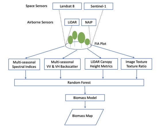
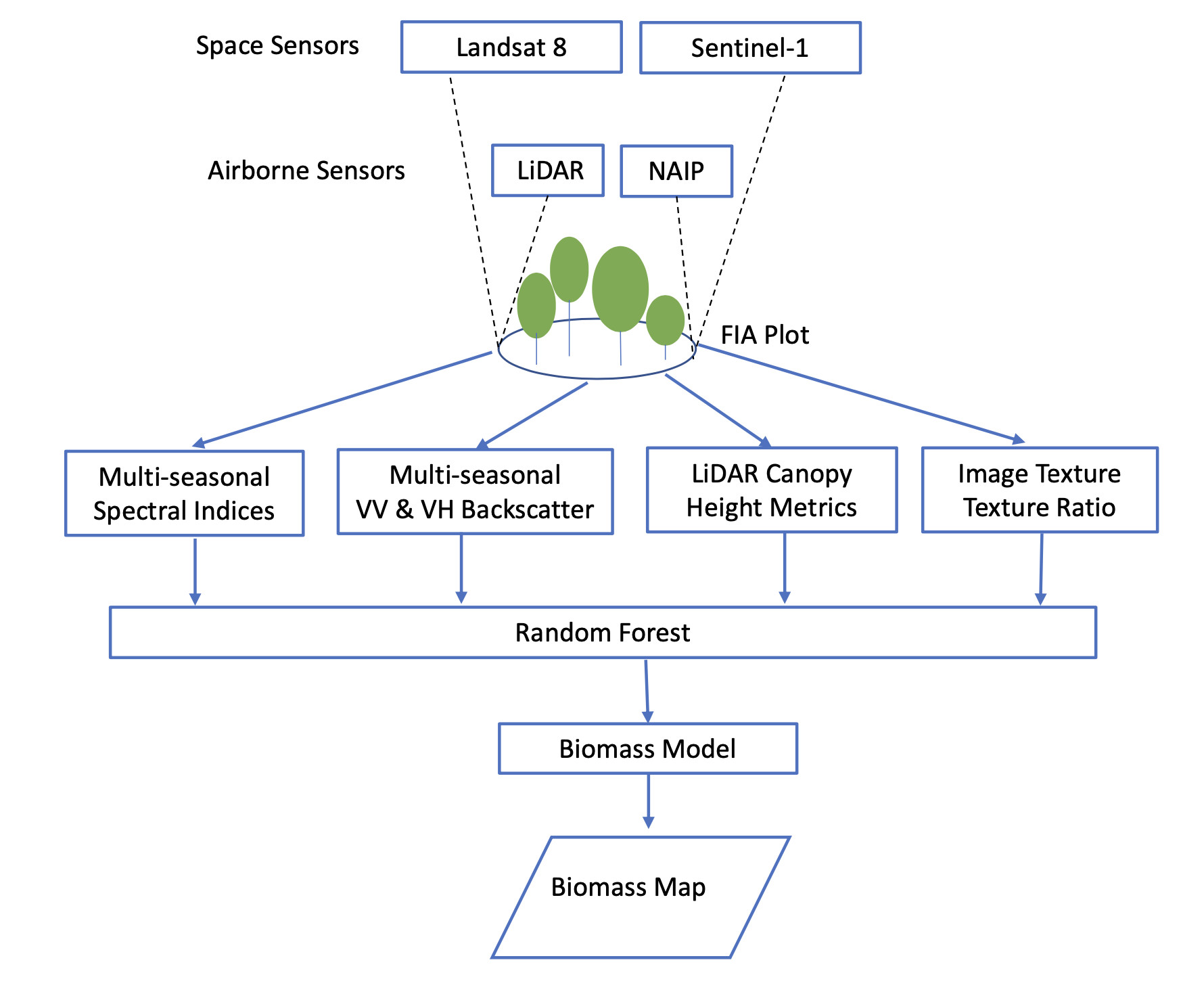
2. Materials and Methods
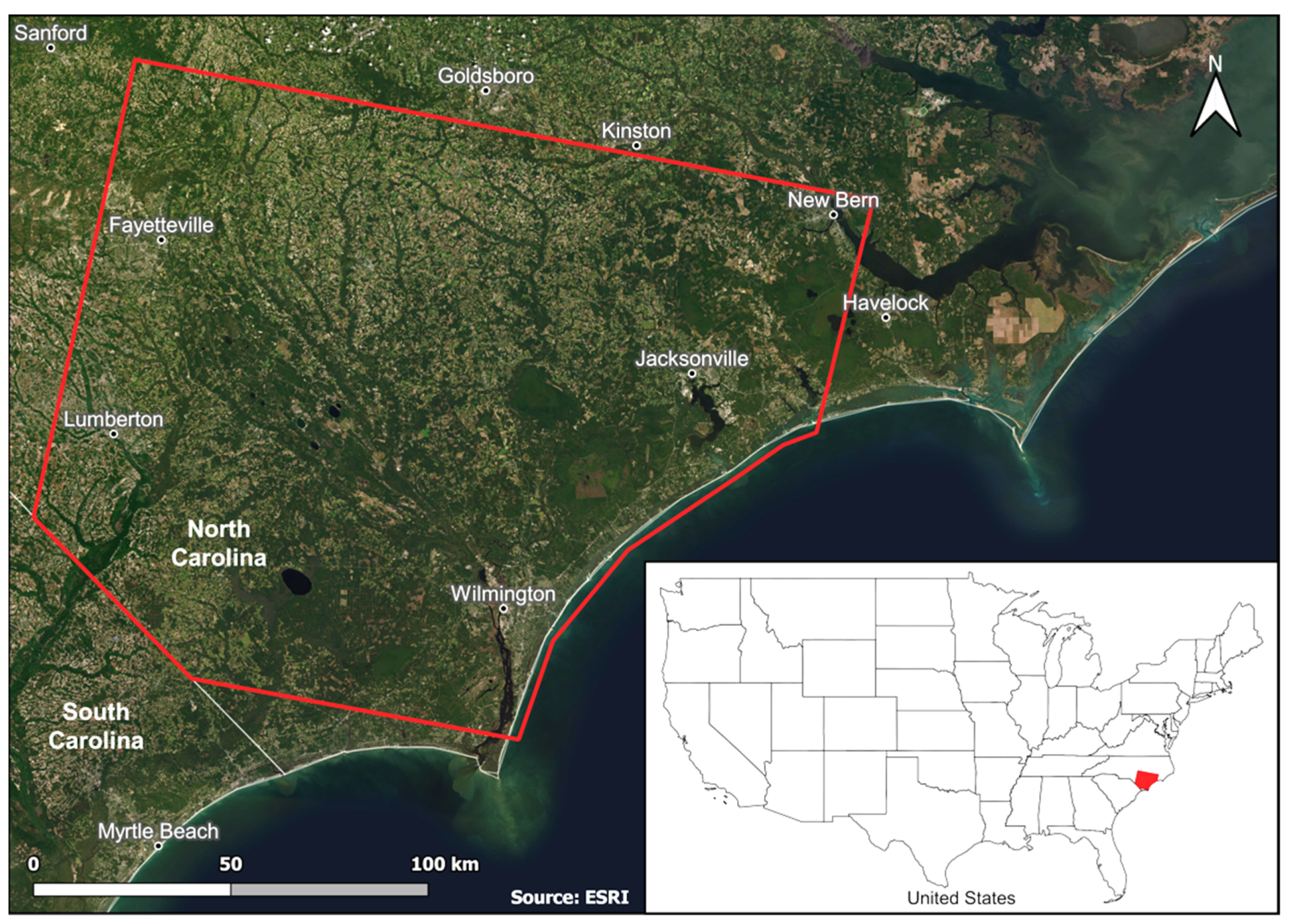
2.1. Study Area

The study area is located in eastern North Carolina (NC), USA, spanning approximately 23,000 km2 covered by a Landsat scene of WGS path = 15, row = 36 (Figure 1). This region belongs to the Southern Coastal Plain, with most vegetation being classified as coniferous forest, dominated by Loblolly pine (Pinus taeda). The majority of counties within this region are over 70% timberland by area, making it an important forest resource. Being most severely hit by Hurricane Florence in 2018, we selected this region to pave the way for an eventual estimation of the impact of the Hurricane on forest biomass. We currently focus on pre-hurricane forest biomass estimation as the post hurricane LiDAR is not yet available.

2.2. Forest Inventory and Analysis Data

We used FAGB derived from U.S. Forest Service Forest Inventory and Analysis (FIA) data. The FIA program collects, analyzes, and reports the status of American Forests for all 50 states of the U.S. and its territories and possessions (http://fia.fs.fed.us, accessed on 5 February 2022). The FIA program designed a national hexagon grid covering 50 states with each hexagon spanning 5937 acres (~2404 ha) in area and contain a randomly located plot [52]. Each FIA plot consists of four 7.3 m radius subplots, with one located in the plot center, and the centers of the other three subplots are 120 ft (36 m) away from the center plot distributed 120 degrees from each other [53]. Because our LiDAR data were collected in 2014, plots that were sampled in 2013, 2014, and 2015 within the study area were used as the reference for model development and evaluation. The sum of the aboveground biomass for all trees within a sampling plot with DBH greater than 5 inches (i.e., 12.7 cm) makes up the total FAGB for the plot. We selected the FIA sampling plots in this study that fall into the forest land cover based on the USGS National Land Cover Dataset [54] with aboveground forest biomass carbon greater than zero and the 95th percentile height greater than ten feet (~3 m). After applying these exclusion criteria, the remaining 227 plots in the study area are available for model training and testing.
To ensure the privacy of private landowners and to protect plots from vandalism, the locations of the plots within the publicly available FIA database are fuzzed and swapped. To overcover the confidentiality of the accurate FIA plot locations, our USFS collaborators helped extract the multisource remotely sensed data for plot locations using the accurate plot coordinates and then provided us a table that contains the plot attributes (including biomass) and the extracted remotely sensed data without the accurate plot coordinates to the rest of the research team. This essentially provided this study with access to the data with their precise locations without anyone outside of USFS accessing the confidential information [51].

2.3. Remote Sensing Data

2.3.1. LiDAR Data

We used airborne LiDAR to provide canopy height information. The statewide discrete return LiDAR data used in this study were collected as part of a joint project by the NC Risk Management Office, NC Department of Transportation, and other state collaborators (available for download at https://sdd.nc.gov/, accessed on 5 February 2022). The LiDAR data were collected in the Spring of 2014 in the leaf-off condition with no snow on the ground. The data were collected using a combination of airborne Leica ALS70HP-II and Optech Pegasus HA500 sensors at a resolution of 2 points per square meter. The NC Risk Management Office provided the LiDAR data in the LAS version 1.3 standard format with associated 5-foot resolution DEMs in a 5000-foot by 5000-foot tiling scheme or ~1.5 × 1.5 km.
Using the 5-foot (~1.5 m) DEMs, the LiDAR data were first normalized to the ground, i.e., the height measurements in the LiDAR data are heights from the ground. The normalized LiDAR data were then used to calculate a set of height metrics, each representing height at 25, 50, 75, 85, and 95% of points within the 30 m spatial resolution. These height metrics represent the vertical canopy structure, which are used as variables associated with FAGB. The percentiles used for analysis were chosen to characterize the upper canopy containing the majority of biomass and to eliminate extreme height values due to sensor errors and undesirable interactions.

2.3.2. RaDAR Data

The European Space Agency’s (ESA) Sentinel-1 mission comprises two polar-orbiting satellites with a relative azimuth angle of 180° from each other, Sentinel-1A and Sentinel-1B, each of which is equipped with the Synthetic Aperture Radar (SAR) instrument for collecting surface backscatter in the C-band in multiple modes and in dual-polarization (VV + VH, HH + HV). The use of the C-band allows the acquisition of imagery day and night and in all weather conditions. Two Sentinel-1 scenes were acquired for this study, one dated 3 March 2015, representing winter leaf-off conditions, and one dated 18 August 2015, representing summer leaf-on conditions. The Sentinel-1 scenes were retrieved as the Level-1 High Resolution (roughly 10-m) Ground Range Detected (GRD) Interferometric Wide (IW) Swath mode data product in the VV and VH polarizations from ESA’s Copernicus Open Access Hub (https://scihub.copernicus.eu/, accessed on 5 February 2022).
A standard Sentinel-1 GRD preprocessing workflow was applied to process the images acquired for this study. All Sentinel-1 preprocessing was conducted in the ESA’s own Sentinel Applications Platform (SNAP). Accurate orbit information was applied, thermal noise was removed, digital pixel values were converted into radiometrically calibrated SAR backscatter, a Lee-Sigma speckle filter was applied, range-doppler terrain correction was performed, and the unitless backscatter was converted to backscatter coefficient in decibels using a logarithmic transformation. Border noise removal performed through SNAP does not adequately work on Sentinel-1 images captured before March 2018. As a result, border noise was manually cropped from the images where needed.

2.3.3. Multispectral Data

Landsat 8 Analysis Ready Data (ARD) data, retrieved from the USGS Earth Explorer data portal (https://earthexplorer.usgs.gov/, accessed on 5 February 2022), were used in this study. We used two images representing the leaf-on and leaf-off conditions similar to the RaDAR data. These images capture species composition information for image classification [55,56]. The leaf-off condition image was acquired on 6 February 2015, and the leaf-on condition image was on 30 June 2015. Both images were almost cloud-free, but any clouded or nonclear pixels were masked out using the pixel quality assessment band. The bands used for this analysis include Band 2 (Visible Blue), Band 3 (Visible Green), Band 4 (Visible Red), Band 5 (Near-Infrared), Band 6 (Shortwave Infrared 1), and Band 7 (Shortwave Infrared 2). We first conducted the Tasseled Cap (TC) transformation for each image and used the brightness, greenness, and wetness components in the biomass model, instead of the six original bands. Three vegetation indices were further derived, including Normalized Difference Vegetation Index (NDVI, Equation (1)), Enhanced Vegetation Index (EVI, Equation (2)), and Structural Index (SI, Equation (3)) [57]. These vegetation indices, along with the TC brightness, greenness, and wetness, represent the data input from the optical sensor.
N D V I = ρ N I R ρ R e d ρ N I R + ρ R e d   ,
E V I = G ( ρ N I R ρ R e d ) ρ N I R 6.0 ρ B l u + 7.5 ρ R e d + 1   ,
S I = ρ M I R ρ N I R   ,
where ρ B l u , ρ R e d , ρ N I R , ρ M I R are surface reflectance for blue, red, near-infrared, and mid-infrared bands, respectively.

2.3.4. Very High-Resolution Optical Imagery

The Very-High-Resolution (VHR) imagery for this study was derived from the National Agriculture Imagery Program (NAIP) under the USDA Farm Service Agency (https://www.fsa.usda.gov/programs-and-services/aerial-photography/, accessed on 5 February 2022). The VHR imagery provided image texture for this study. We used the 4-band visible-infrared aerial imagery collected in the Spring of 2014 with a 1-m spatial resolution to cover the study area. All NAIP imagery was acquired as compressed county mosaics from the USDA’s geospatial data gateway (https://datagateway.nrcs.usda.gov/GDGHome_DirectDownLoad.aspx, accessed on 5 February 2022).
We first conducted a principal component transformation of the NAIP imagery and selected the first principal component, which represents a brightness feature that contains information from all bands. The first principal component contains more information in the image than any of the original bands or other principal components. Second, the first principal component image was further resampled to 2 m and 3 m spatial resolutions, and the local texture was calculated for the 1, 2 and 3 m spatial resolution first principal component images. Third, the local variance calculated at 1, 2 and 3 m spatial resolutions were downscaled to 30 m spatial resolution with simple averaging. Fourth, we calculated the ratio (i.e., Equation (4)) of degraded image texture at 30 m spatial resolution with initial image texture derived at the 2 m spatial resolution to that at the 3 m spatial resolution because this ratio correlates with mean stand crown diameter, which in turn strongly relates to DBH [51,58].
R 2 / 3 = T 2   ×   2 T 3   ×   3 ,
where T2×2 is the image texture calculated at 2 m spatial resolution and downscaled to 30 m spatial resolution with simple average; T3×3 is the image texture calculated at 3 m spatial resolution and downscaled to 30 m spatial resolution with simple average. R2/3 is the ratio of T2×2 to T3×3. Eventually, we derived two layers of spatial data both at 30 m spatial resolution as the model inputs, i.e., the image texture initially calculated at the 1 m spatial resolution, and the ratio of image variance at 2 m to that of 3 m.

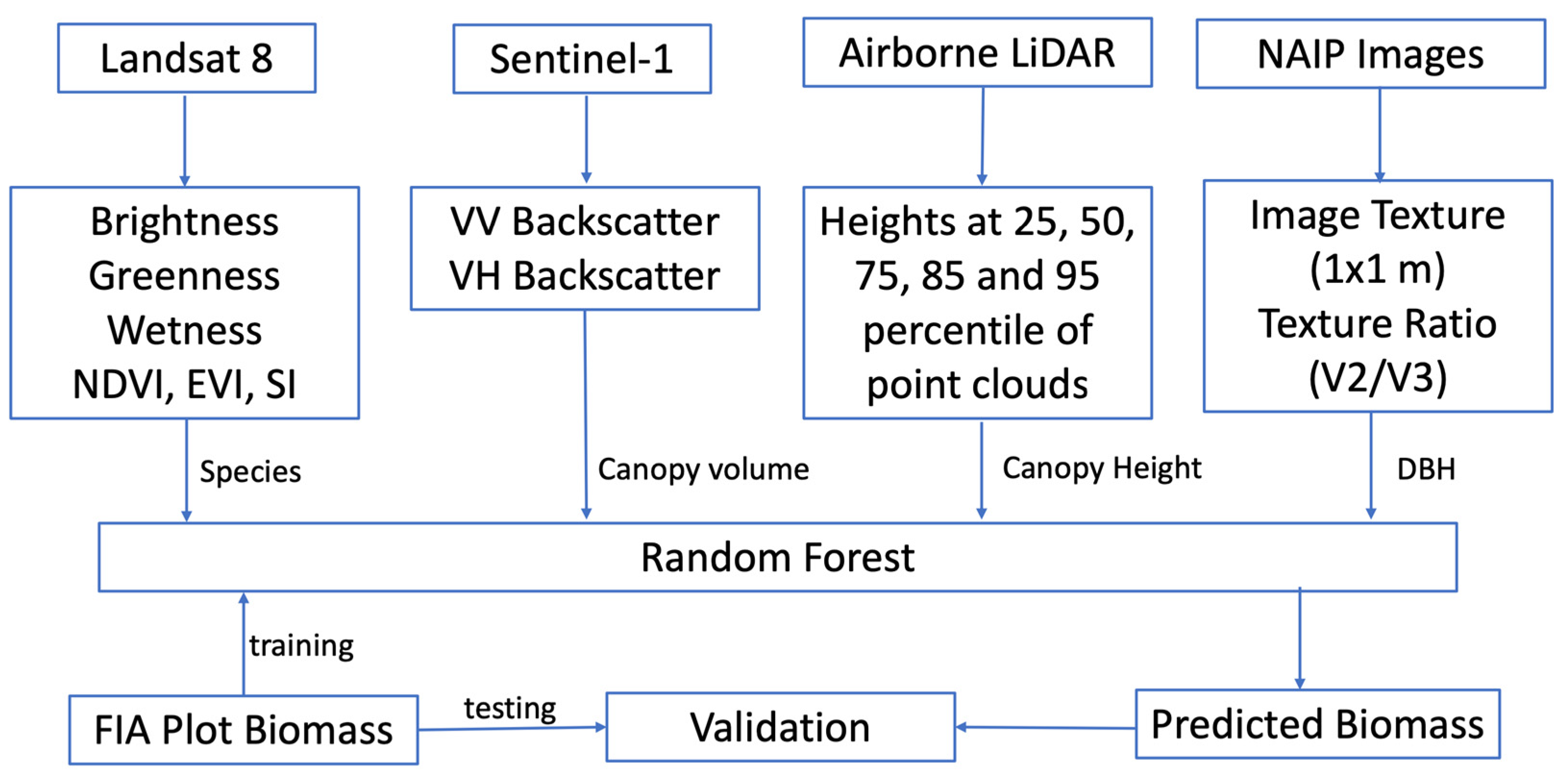
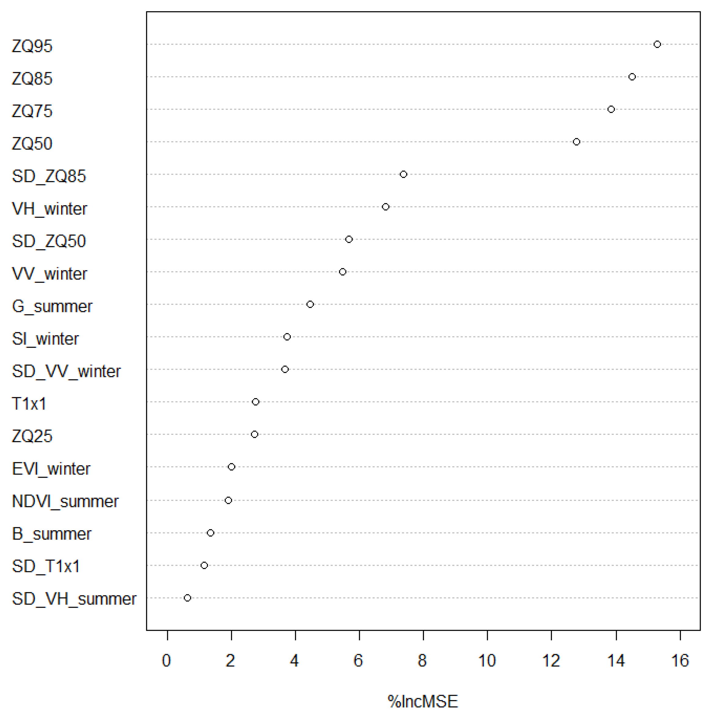
2.4. Biomass Model with Random Forest
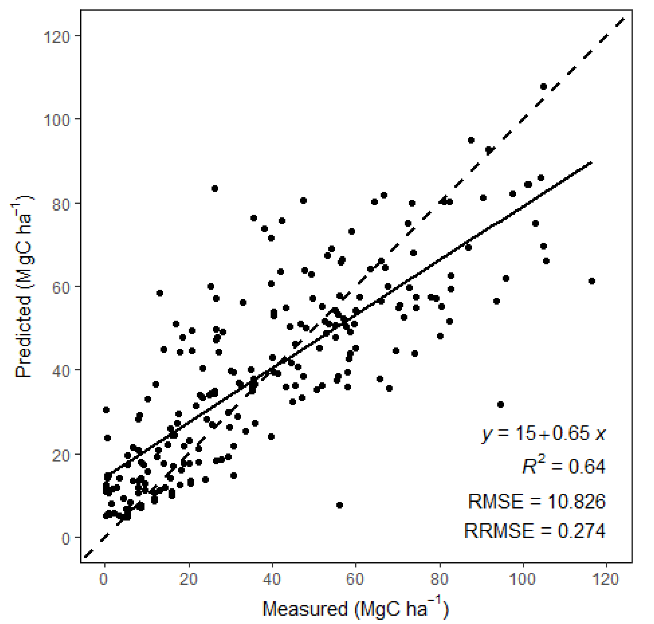
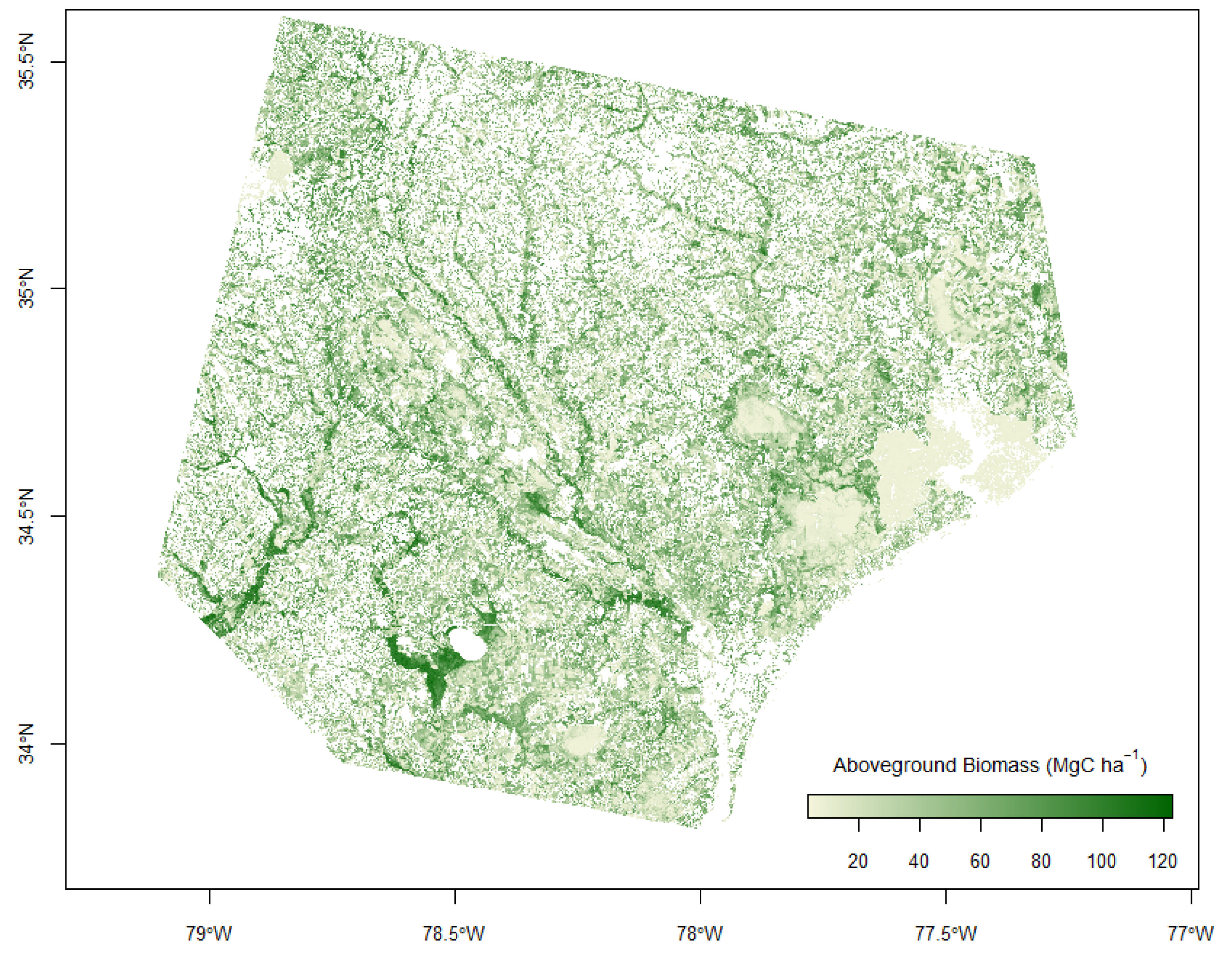
We developed our biomass model based on Random Forest (RF), a machine learning algorithm that can be used for both classification and regression [59]. A “tree” in the “forest” is established from a bootstrapped sample from the reference data with the remaining reference data left “out-of-bag”, which are used to derive the relative importance of each of the input features, making it easy to compare predictor variables and determine the most useful set for regression. RF is not as susceptible to overfitting as an individual tree [59,60], and it is especially effective in capturing nonlinearity and interactions among the predictive variables [61]. In addition, RF models are relatively robust to noise in training data. For this implementation of random forest, variable importance is measured as the percent increase in mean squared error that results in the exclusion of the given variable. The general workflow is shown in Figure 2.
We tested many RF models, each with a different set of independent variable combinations. Each model run produces a degree of fitness, i.e., R2, and the root mean squared error (RMSE) based on the “out-of-bag” samples. We selected the model that predicts the aboveground biomass with the highest R2 and smallest RMSE. Finally, we evaluated the selected RF model with a predicted FAGB map and the biomass from all FIA plots within the study area.
Table 1 lists all remote sensing features derived from LiDAR, RaDAR (Sentinel-1), multispectral (Landsat 8), and very high-resolution (NAIP) data that were used for biomass mapping with RF. Due to the large number of feature variables, we implemented an automatic feature selection with KnowGRRF, which is an R package developed by Guan and Liu [62] for statistical computation, to identify the most important remotely sensed predictors for biomass estimation. In order to use KnowGRRF, we first need to generate a regularization coefficient for each variable by running the RF to map FAGB with all variables included. The regularization coefficient for each variable is calculated using Equation (5) based on the variable importance value from the initial RF run.
C j = 0.5 + 0.5   ( I j I m a x ) ,
where Cj is the regularization coefficient for the jth variable; Ij is the importance value of jth variable generated by the initial RF model, and Imax is the maximum importance value from the initial RF model. After we generated the regularization coefficient for each variable, we used KnowGRRF to eliminate the least important variable following a stepwise model based on the Akaike Information Criterion (AIC). Due to the randomness of bootstrapping in RF, there will be some variations in the outputs from different model runs. To produce a robust feature selection, the KnowGRRF was run 100 times. Based on the frequency of feature selection in the 100 runs, the variables were added sequentially from the most frequently selected ones and gradually adding the less frequently selected variables from the 100 model runs, and the final set of features was selected based on the smallest AIC values [62]. We also tested the effect of the sample size on the robustness of the model output. We tested the final model with two-thirds, half, and one-third of the FIA biomass data. We ran the model 50 times for each subset of the samples, and each time we randomly selected the desired subset of plot samples as input to the model. We analyzed the out-of-bag R2 and RMSE from these model outputs to evaluate the model performance.
In addition to automatic feature selection using KnowGRRF for the final biomass mapping model, we tested the performance of various subsets of the remotely sensed data with RF. Sub-datasets included data from each sensor, i.e., LiDAR, RaDAR, multispectral, and very-high resolution aerial imagery, as well as the combination of the RaDAR and multispectral data split by the season they were acquired. The overall performance of each model was evaluated based on selected features that maximized accuracy while reducing the overall number of inputs. The number of trees contained in each RF model was set to 300, sufficiently high to allow all input rows to be used multiple times in model development and to produce a stable output.

3. Results

The automatic feature selection R package, KnowGRRF, selected 18 variables from Table 1 based on AIC. Figure 3 shows the importance order of these 18 variables. The top five most important variables are all from the lidar height metrics, including ZQ95, ZQ85, ZQ75, ZQ50, and SD_ZQ85. In addition, ZQ25 and SD_ZQ50 from the LiDAR sensor also made it to the model, although they were not as important. For multispectral remotely sensed features from Landsat 8, the selected features include G_summer, SI_winter, EVI_winter, NDVI_summer, and B_summer. Thus, the multiseasonal optical images are valuable for biomass mapping. For features from the RaDAR sensor, VH_winter, VV_winter, SD_VV_winter, and SD_VH_summer were selected into the model. Moreover, VH_winter is the most important variable not from the LiDAR sensor in the model. It is understandable why VH_winter, not VH_summer, was selected because the short wavelength C-band from Sentinel-1 cannot penetrate much into the canopy in the summer when the forest canopies are dense. Variables from the VHR image include T1×1 and SD_T1×1, which are related to tree crown size. Therefore, all four types of data made it into the final model, indicating the validity of our conceptual model.
The variable importance values provided by RF (Figure 3) indicate the top four most important variables are the ZQ95, ZQ85, ZQ75, and ZQ50 canopy height of total LiDAR returns, followed by SD_ZQ85 of LiDAR points. Among the height metrics, the height of the 95th percentile LiDAR points is the most important height metric. The subsequent highly important feature after the height metrics is RaDAR backscatter intensity from the VH polarization in the wintertime. Although VV_winter and SD_VV_winter also enter the model, they are not important as VH_winter. Summer backscatter intensity do not enter the model, but only SD_VH_summer is selected, ranking last in its importance among the variables selected. The features from the Landsat 8 imagery include G_summer, SI_winter, EVI_winter, NDVI_summer, and B_summer in order of importance. Variables selected from NAIP include T1×1 and SD_T1×1 with relatively low importance ranking. Surprisingly R2/3 do not enter the model. This may be because of the relatively low aboveground forest biomass (Figure 4) with relatively small trees. Thus, the spatial information is not very helpful in mapping the biomass. For this model, the parameter ‘mtry’, the number of variables considered at each split within a tree, was tested to produce the highest accuracy. By testing every possible value of ‘mtry’ for the highest model accuracy, we find that the model leads to the most accurate prediction when ‘mtry’ is set to five.
The selected model yields an R2 of 0.625 with an RMSE of 18.8 Mg/ha (47.6%) based on the “out-of-bag” samples. When using the selected model to produce the biomass map and validated with the biomass from all the FIA plots, the R2 increased to 0.64 with the regression RMSE = 10.8 Mg/ha (Figure 4), which is smaller than the RMSE based on the “out-of-bag” samples. The R2 for the whole sample was slightly higher than the out-of-bag sample because each plot would be “seen” by some of the trees in the RF, increasing the R2. The out-of-bag samples are not seen by any of the “trees” in the training process; thus, it is a more rigorous validation. Figure 4 shows that the predicted biomass and the FIA biomass distribute well along the 1:1 line. There is a slight overestimation of biomass for plots with low biomass and an underestimation for plots with high biomass.
To understand the contribution of each sensor to biomass mapping, we tested its respective predictive power with the data (Table 2). When all variables are included, the model performance is not as good as the parsimonious model after eliminating the less important variables. Among all the different types of data, the performance of features from the LiDAR sensor dwarfed all other sensors. It is not surprising that the top five most important variables are all from the LiDAR sensor. The performances of multiseasonal features from RaDAR and multispectral sensors are similar, with an R2 of 0.065. It is interesting to notice that the Tasseled Cap transformation components have much higher R2. Vegetation indices alone performed much poorer than the Tasseled Cap components.
The effects of sample size with our final model on mapping FAGB is shown in Table 3, which shows basic statistics of the 50 model runs for each subset of the samples. As expected, the models with the smaller subsamples have a lower R2, larger variation in R2 among different model runs, and consequently produced a larger out-of-bag RMSE and larger variation in RMSE. As demonstrated in Table 3, the model is very robust to the variation in sample sizes. The out-of-bag R2 decreased only 0.044 using only one-third of the whole sample, and the RMSE increased by 1.0 Mg/ha. Therefore, we can safely say that our model results are robust.
Using the selected RF model, we produced the forest aboveground biomass map as shown in Figure 5, on which we masked out nonforest areas based on the 2016 land-cover map from the National Land Cover Dataset [54]. The area is dominated by agricultural land, and we do not see a large expanse of land with high biomass. We can see that the highest biomass is distributed in the riparian zones, partly because these areas are strictly protected from logging and partly because the abundance of nutrients and water that favorably supports forest growth over the areas that are further away from the riparian zones.

4. Discussion

This study used remotely sensed data from multiple sensors, including Landsat 8, airborne LiDAR, Sentinel-1 RaDAR, and very high-resolution optical imagery from the National Agriculture Imagery Program. Multiseasonal Landsat 8 imagery was intended to capture the species variation in space; LiDAR height metrics to describe vertical canopy structure; Sentinel-1 RaDAR backscatter in the C-band in dual-polarization (VV and VH) for both winter and summer seasons to capture the canopy volume; the image texture from very high-resolution optical imagery to provide texture measures of forest canopies as well as the ratio of the image texture of 2 m to that of 3 m spatial resolution. However, the importance ranking information provided by the RF model showed the height metrics dominate all other variables. Moreover, it is not the height at a single energy level, but the entire height profile. This finding is different from a previous study that found the height of the median energy, i.e., the height where the 50th percentile of LiDAR data points from the ground, was the most important variable [42]. The forests in the study area here are primarily Loblolly pine stands with relatively simple canopy structures, making ZQ95 the most important canopy height metric in biomass mapping, but heights at other energy levels are also important for biomass mapping. The height metrics alone capture 59.5% of the variance in biomass, compared to 62.5% from the full model. The importance of canopy height in biomass mapping is consistent with findings in the literature [41,42,63,64,65]. The performance of our model is equivalent to other studies using RF with multiple sources of data mapping biomass [63,66]. Despite the robust model performance, there remains some systemic bias in the biomass estimation, i.e., a slight overestimation at the lower end and an underestimation at the higher end of biomass. Such a bias pattern is a common issue for remotely sensed biomass estimation in other studies [50,66].
Unlike other land surface biophysical parameters, such as leaf area or canopy height, that can be measured directly from remotely sensed signals, there is no direct remotely sensed signal for biomass [32]. Remote sensing only measures biomass proxies that are imperfectly related to biomass, such as canopy height and species composition. The leaf area index in the canopy had been used to measure biomass fairly effectively [28]. However, the leaf area index of forest canopies saturates within a couple of decades, whereas forest biomass can continue to increase for centuries [24]. Among the biomass proxy variables measured remotely, the relationship of vegetation canopy height does not saturate with FAGB. Therefore, canopy height from LiDAR sensors has proved to be the most important variable for biomass mapping [67]. However, the height–biomass relationship is species-dependent, as is a well-known fact in allometry [14,15,68]. Although reports used optical sensors alone that produced reliable biomass maps, these studies are generally based on coarse resolution remotely sensed data [50,69,70]. The relative success of using the optical sensors in mapping forest biomass over a large area using coarse resolution imagery is primarily driven by the vegetation cover effect. Such an approach may not apply to higher spatial resolution applications. Many localized studies found that optical sensors alone cannot accurately map biomass beyond 150 Mg/ha [33], and the Root Mean Squared Error (RMSE) for biomass mapping can be as high as 50% or higher [28,71]. As a result, many studies used remotely sensed data from multiple sensors.
Tremendous efforts were also dedicated to mapping forest aboveground biomass using RaDAR data because RaDAR signals can penetrate clouds, which are a constant impediment to biomass mapping using optical images, particularly in the tropics. An early attempt to map forest aboveground biomass with RaDAR was conducted with NASA/JPL SAR data [35,36], and they found that RaDAR backscatter intensity of P-band best correlated with biomass, and the relationship decreases with increasing frequencies. Moreover, they found that the cross-polarized backscatter intensity best explains the forest biomass variation [36,39]. However, RaDAR signals saturate with biomass at about 200 Mg/ha for P-band, 100 Mg/ha for L-band, and C-band backscatter is much less sensitive to forest aboveground biomass variation. Soil and vegetation moisture can have a stronger influence on high frequency (X or C-band) backscatter RaDAR signals than FAGB [37,72]. These findings were later confirmed by Luckman et al. [73]. Recently, Liao et al. [74] compared coherence magnitude, interferometric phase, and backscatter signals of P-band PolInSAR from TropiSAR to map forest aboveground biomass and found the volume backscatter from the forest canopy best predicts tropical FAGB. Two promising RaDAR instruments, BIOMASS with a full polarimetric P-band SAR to be launched by the European Space Agency in 2023 and NISAR with L- and S-band SAR also to be launched in 2023 by a joint U.S.-India effort [75], will bring new momentum in mapping FAGB with RaDAR data in the near future.
Given the complexity of remotely sensed signal interactions with land surface conditions, it seems no single sensor can provide data that can reliably map FAGB. Most recent efforts in mapping forest aboveground biomass almost all engage with remotely sensed data from multiple sensors. Blackard et al. [16] produced the nationwide forest biomass for the U.S. using MODIS remote sensing data and data products as well as topographic, climatic variables, and other ancillary data. However, this biomass map tends to overestimate low biomass and underestimate high biomass. Animi and Sumantyo [76] found that biomass estimation accuracy based on a multilayer perceptron neural network model was significantly better when using both RaDAR and optical data than either alone. Huang et al. [66] and Cutler et al. [77] found that RaDAR image texture significantly improved biomass mapping with Landsat TM data. Image texture for both optical and RaDAR sensors, SD_VV_winter, SD_VH_Summer, and T1×1_ were selected into our final model using an automatic feature selection algorithm, KnowGRRF, based on AIC in this study. Similarly, synergistic use of optical and LiDAR data also improves the accuracy of biomass mapping [78,79,80]. More recently, Brovkina et al. [81] used airborne hyperspectral and LiDAR data to map FAGB in central Europe and found that the biomass maps estimated using both data simultaneously were much more accurate than using either datum alone. Andersen et al. [82] and Babcock et al. [67] found that stratifying LiDAR data based on land cover derived from optical sensors improved the biomass mapping accuracy in interior Alaska, USA. There is strong evidence in the literature that using remotely sensed data from multiple sensors enhances the accuracy of biomass mapped. This paper proposes to use data from multiseasonal optical, multiseasonal RaDAR, LiDAR, and very high-resolution data to map FAGB. These data provide information related to forest species, canopy volume, canopy height, and DBH, which are the key data needed to estimate individual tree biomass on the ground. Therefore, the use of data from multiple sensors that provide information on these factors should be the theoretical basis for mapping FAGB with remote sensing. Its potential has not been fully demonstrated in this study. More studies are needed to test this mapping algorithm in areas with a higher biomass density and more heterogeneity species variation because the variables accounting for the effects of tree crown size and species variation did not fully realize their potential in this study.

5. Conclusions

This study proposes a conceptual model to map aboveground forest biomass using remotely sensed data. The new conceptual model posits that we need remotely sensed data to provide information about species composition, canopy height, and diameter at breast height. We test the conceptual model by fusing optical medium resolution data from Landsat, very high-resolution images from USDA NAIP, airborne LiDAR, and RaDAR images from Sentinel-1 to map aboveground forest biomass. Our final model is able to explain 62.5% of the biomass variation and the RMSE of the model is 18.5 Mg/ha (47.6%) calculated from out-of-bag samples. We find that the LiDAR height metrics are the most important variables. We need the height profile for the 95th, 85th, 75th, 50th, and 25th percentile canopy heights of the LiDAR points in mapping the biomass, rather than a single height metric. The importance of height metrics dwarfs all other variables, although the inclusion of Landsat, very high-resolution imagery, and the RaDAR data from Sentinel-1 only marginally improves the performance of the model. The lack of importance from multiseasonal optical imagery in aboveground forest biomass mapping in this study is likely due to the dominance of evergreen pine forests in the region. The lack of significant contribution from Sentinel-1 C-band SAR backscatter is consistent with the literature because C-band has a limited capacity to penetrate the canopy. The limited contribution from the image texture from USDA NAIP imagery deserves further investigation because biomass for these FIA plots is relatively low. In addition, we find that our model is robust because its performance is not sensitive to minor changes in training sample size. More studies are needed to further test the conceptual model for aboveground biomass mapping in areas with a broader biomass range and a more diverse species composition.

Author Contributions

Conceptualization, C.S., J.C. and C.W. (Curtis Woodcock); Data curation, D.E. and J.C.; Formal analysis, D.E., C.S., C.W. (Chao Wang); Funding acquisition, T.P., E.F. and C.S.; Methodology, D.E., C.W. (Chao Wang) and C.S.; Resources, C.S., C.W. (Chao Wang); Validation, D.E. and J.C.; Writing—original draft, C.S., D.E.; Writing—review & editing, D.E., C.W. (Chao Wang), J.C., Y.Z. and E.F. All authors have read and agreed to the published version of the manuscript.

Funding

This work is partly supported by a NASA grant (NNX17AE69G), an internal Creativity Hub grant from the University of North Carolina at Chapel Hill awarded to Carolina Population Center, and an NSF Growing Convergence Research Grant (NSF 2021086).

Institutional Review Board Statement

Not applicable.

Data Availability Statement

The biomass data and the corresponding remote sensing data for the FIA plots are downloadable at http://csong.web.unc.edu, accessed on 5 February 2022. The locations for the FIA plots are confidential data, not available to the public.

Acknowledgments

We thank GIS Analyst, John Lay, at the North Carolina Floodplain Mapping Program for providing the 2014 LiDAR data used in this study.

Conflicts of Interest

The authors declare no conflict of interest.

References

  1. IPCC. Summary for Policymakers. In Climate Change 2021: The Physical Science Basis. Contribution of Working Group I to the Sixth Assessment Report of the Intergovernmental Panel on Climate Change; MassonDelmotte, V., Zhai, P., Pirani, A., Connors, S.L., Péan, C., Berger, S., Caud, N., Chen, Y., Goldfarb, L., Gomis, M.I., et al., Eds.; IPCC: Geneva, Switzerland, 2021. [Google Scholar]
  2. Luthi, D.; Le Floch, M.; Bereiter, B.; Blunier, T.; Barnola, J.; Siegenthaler, U.; Raynaud, D.; Jouzel, J.; Fischer, H.; Kawamura, K.; et al. High-resolution carbon dioxide concentration record 650,000–800,000 years before present. Nature 2008, 453, 379–382. [Google Scholar] [CrossRef] [PubMed]
  3. Lindsey, R. Climate Change: Atmospheric Carbon Dioxide. 2020. Available online: http://www.climate.gov/news-features/understanding-climate/climate-change-atmospheric-carbon-dioxide (accessed on 5 February 2022).
  4. Houghton, R.A. Land-use change and the carbon cycle. Glob. Chang. Biol. 1995, 1, 275–287. [Google Scholar] [CrossRef]
  5. Tian, H.; Lu, Q.; Ciais, P.; Michalak, A.M.; Canadell, J.G.; Saikawa, E.; Huntzinger, D.N.; Gurney, K.R.; Sitch, S.; Zhang, B.; et al. The terrestrial biosphere as a net source of greenhouse gases to the atmosphere. Nature 2016, 531, 225–228. [Google Scholar] [CrossRef] [PubMed] [Green Version]
  6. Cohen-Shacham, E.; Walters, G.; Janzen, C.; Maginnis, S. (Eds.) Nature-Based Solutions to Address Global Societal Challenges; IUCN: Gland, Switzerland, 2016; Volume xiii, p. 97. ISBN 978-2-8317-1812-5. [Google Scholar] [CrossRef] [Green Version]
  7. Le Quere, C.; Andrew, R.M.; Friedlingstein, P.; Sitch, S.; Hauck, J.; Pongratz, J.; Pickers, P.A.; Korsbakken, J.I.; Peters, G.P.; Canadell, J.G.; et al. Global carbon budget 2018. Earth Syst. Sci. Data 2018, 10, 2141–2194. [Google Scholar] [CrossRef] [Green Version]
  8. Allen, C.D.; Macalady, A.K.; Chenchouni, H.; Bachelet, D.; McDowell, N.; Vennetier, M.; Kitzberger, T.; Rigling, A.; Breshears, D.D.; Hogg, E.T.; et al. A global overview of drought and heat-induced tree mortality reveals emerging climate change risks for forests. For. Ecol. Manag. 2010, 259, 660–684. [Google Scholar] [CrossRef] [Green Version]
  9. Choat, B.; Jansen, S.; Brodribb, T.J.; Cochard, H.; Delzon, S.; Bhaskar, R.; Bucci, S.J.; Feild, T.S.; Gleason, S.M.; Hacke, U.G.; et al. Global convergence in the vulnerability of forests to drought. Nature 2012, 491, 751–756. [Google Scholar] [CrossRef] [Green Version]
  10. Ciais, P.; Reichstein, M.; Viovy, N.; Granier, A.; Ogee, J.; Allard, V.; Aubinet, M.; Buchmann, N.; Bernhofer, C.; Carrara, A.; et al. Europe-wide reduction in primary productivity caused by the heat and drought in 2003. Nature 2005, 437, 529–533. [Google Scholar] [CrossRef]
  11. Kurz, W.A.; Dymond, C.C.; Stinson, G.; Rampley, G.J.; Neilson, E.T.; Carroll, A.L.; Ebata, T.; Safranyik, L. Mountain pine beetle and forest carbon feedback to climate change. Nature 2008, 452, 987–990. [Google Scholar] [CrossRef]
  12. Song, C. Optical remote sensing of forest leaf area index and biomass (invited progress report). Prog. Phys. Geogr. 2013, 37, 98–113. [Google Scholar] [CrossRef]
  13. Zhai, B.; Song, C.; Zhang, H.; Wang, W. Studies on Biomass and productivity of Pinus Tabulaeformis plantation at a Permanent Ecosystem Plot in Taiyue forest region Shanxi Province. J. Beijing For. Univ. 1992, 14, 156–163, (In Chinese with English Abstract). [Google Scholar]
  14. Gholz, H.L.; Grier, C.C.; Campbell, A.G.; Brown, A.T. Equations for Estimating Biomass and Leaf Area of Plants in the Pacific Northwest; Forest Research Laboratory, School of Forestry, Oregon State University: Corvallis, OR, USA, 1979; Available online: https://ir.library.oregonstate.edu/concern/technical_reports/bn999796n?locale=en (accessed on 5 February 2022).
  15. Jenkins, J.C.; Chojnacky, D.C.; Heath, L.S.; Birdsey, R.A. Comprehensive Database of Diameter-Based Biomass Regressions for North America Tree Species; General Technical Report NE-319; USDA Forest Service: Washington, DC, USA, 2004.
  16. Blackard, J.A.; Finco, M.V.; Helmer, E.H.; Holden, G.R.; Hoppus, M.L.; Jacobs, D.M.; Lister, A.J.; Moisen, G.G.; Nelson, M.D.; Riemann, R.; et al. Mapping US forest biomass using nationwide forest inventory data and moderate resolution information. Remote Sens. Environ. 2008, 112, 1658–1677. [Google Scholar] [CrossRef]
  17. Nelson, R.; Margolis, H.; Montesano, P.; Sun, G.; Cook, B.; Corp, L.; Anderson, H.; deJong, B.; Pellat, F.P.; Fickel, T.; et al. Lidar-based estimates of aboveground biomass in the continental US and Mexico using ground, airborne, and satellite observations. Remote Sens. Environ. 2017, 188, 127–140. [Google Scholar] [CrossRef] [Green Version]
  18. Saatchi, S.S.; Harris, N.L.; Brown, S.; Lefsky, M.; Mitchard, E.T.; Salas, W.; Zutta, B.R.; Buermann, W.; Lewis, S.L.; Hagen, S.; et al. Benchmark map of forest carbon stocks in tropical regions across three continents. Proc. Natl. Acad. Sci. USA 2011, 108, 9899–9904. [Google Scholar] [CrossRef] [PubMed] [Green Version]
  19. Lu, D.; Chen, Q.; Wang, G.; Liu, L.; Li, G.; Moran, E. A survey of remote sensing-based aboveground biomass estimation methods in forest ecosystems. Int. J. Digit. Earth 2016, 9, 63–105. [Google Scholar] [CrossRef]
  20. Potter, C.S.; Randerson, J.T.; Field, C.B.; Matson, P.A.; Vitousek, P.M.; Mooney, H.A.; Klooster, S.A. Terrestrial ecosystem production: A process model based on global satellite and surface data. Glob. Biogeochem. Cycles 1993, 7, 811–841. [Google Scholar] [CrossRef]
  21. Running, S.W.; Nemani, R.R.; Heinsch, F.A.; Zhao, M.; Reeves, M.; Hashimoto, H. A continuous satellite-derived measure of global terrestrial primary production. BioScience 2004, 54, 547–560. [Google Scholar] [CrossRef]
  22. Zhang, Y.; Song, C.; Band, L.E.; Sun, G. No proportional increase of terrestrial gross carbon sequestration from the greening Earth. J. Geophys. Res.-Biogeosci. 2019, 124, 2540–2553. [Google Scholar] [CrossRef]
  23. Waring, R.H.; Landsberg, J.J.; Williams, M. Net primary production of forests: A constant fraction of gross primary production? Tree Physiol. 1998, 18, 129–134. [Google Scholar] [CrossRef]
  24. Song, C.; Woodcock, C.E. Estimating Tree crown size from multiresolution remotely sensed imagery. Photogramm. Eng. Remote Sens. 2003, 69, 1263–1270. [Google Scholar] [CrossRef]
  25. Kennedy, R.E.; Ohmann, J.; Gregory, M.; Roberts, H.; Yang, Z.; Bell, D.M.; Kane, V.; Hughes, M.J.; Cohen, W.B.; Powell, S.; et al. An empirical, integrated forest biomass monitoring system. Environ. Res. Lett. 2018, 13, 025004. [Google Scholar] [CrossRef]
  26. Lu, D. The potential and challenge of remote sensing-based biomass estimation. Int. J. Remote Sens. 2006, 27, 1297–1328. [Google Scholar] [CrossRef]
  27. Pflugmacher, D.; Cohen, W.B.; Kennedy, R.E.; Yang, Z. Using Landsat-derived disturbance and recovery history and lidar to map forest biomass dynamics. Remote Sens. Environ. 2014, 151, 124–137. [Google Scholar] [CrossRef]
  28. Zhang, X.; Kondragunta, S. Estimating forest biomass in the USA using generalized allometric models and MODIS land products. Geophys. Res. Lett. 2006, 33, L09402. [Google Scholar] [CrossRef] [Green Version]
  29. Song, C.; Woodcock, C.E.; Li, X. The spectral/temporal manifestation of forest succession in optical imagery: The potential of multitemporal imagery. Remote Sens. Environ. 2002, 82, 285–302. [Google Scholar] [CrossRef]
  30. Luyssaert, S.; Schulze, E.; Borner, A.; Knohl, A.; Hessenmoller, D.; Law, B.E.; Ciais, P.; Grace, J. Old-growth forests as global carbon sinks. Nature 2008, 455, 213–215. [Google Scholar] [CrossRef]
  31. Sader, S.A.; Waide, R.B.; Lawrence, W.T.; Joyce, A.T. Tropical forest biomass and successional age class relationships to a vegetation index derived from Landsat TM data. Remote Sens. Environ. 1989, 28, 143–156. [Google Scholar] [CrossRef]
  32. Song, C.; Dannenberg, M.P.; Hwang, T. Optical Remote Sensing of Terrestrial Primary Productivity (invited progress report). Prog. Phys. Geogr. 2013, 37, 834–854. [Google Scholar] [CrossRef]
  33. Steininger, M.K. Satellite estimation of tropical secondary forest above-ground biomass: Data from Brazil and Bolivia. Int. J. Remote Sens. 2000, 21, 1139–1157. [Google Scholar] [CrossRef]
  34. Chaparro, D.; Duveiller, G.; Piles, M.; Cescatti, A.; Vall-Llossera, M.; Camps, A.; Entekhabi, D. Sensitivity of L-band vegetation optical depth to carbon stocks in tropical forests: A comparison to higher frequencies and optical indices. Remote Sens. Environ. 2019, 232, 111303. [Google Scholar] [CrossRef]
  35. Dobson, M.C.; Ulaby, F.T.; LeToan, T.; Beaudoin, A.; Kasischke, E.S.; Christensen, N. Dependence of Radar Backscatteron Coniferous Forest Biomass. IEEE Trans. Geosci. Remote Sens. 1992, 30, 412–415. [Google Scholar] [CrossRef]
  36. Le Toan, T.; Beaudoin, A.; Riom, J.; Guyon, D. Relating Forest Biomass to SAR Data. IEEE Trans. Geosci. Remote Sens. 1992, 30, 403–411. [Google Scholar] [CrossRef]
  37. Pulliainen, J.T.; Heiska, K.; Hyyppa, J.; Hallikainen, M.T. Backscattering Properties of Boreal Forests at C- and X-Bands. IEEE Trans. Geosci. Remote Sens. 1994, 32, 1041–1050. [Google Scholar] [CrossRef]
  38. Cartus, O.; Santoro, M.; Kellndorfer, J. Mapping forest aboveground biomass in the Northeastern United States with ALOS PALSAR dual-polarization L-band. Remote Sens. Environ. 2012, 124, 466–478. [Google Scholar] [CrossRef]
  39. Hussin, Y.A.; Reich, R.M.; Hoffer, R.M. Estimating Slash Pine Biomass Using Radar Backscatter. IEEE Trans. Geosci. Remote Sens. 1991, 29, 421–425. [Google Scholar] [CrossRef]
  40. Dubayah, R.; Drake, J.B. Lidar Remote Sensing for Forestry. J. For. 2000, 98, 44–46. [Google Scholar]
  41. Lefsky, M.A.; Cohen, W.B.; Acker, S.A.; Parker, G.G.; Spies, T.A.; Harding, D. Lidar Remote Sensing of the Canopy Structure and Biophysical Properties of Douglas-Fir Western Hemlock Forests. Remote Sens. Environ. 1999, 70, 330–361. [Google Scholar] [CrossRef]
  42. Drake, J.B.; Knox, R.G.; Dubayah, R.O.; Clark, D.B.; Condit, R.; Blair, J.B.; Hofton, M. Above-ground biomass estimation in closed canopy Neotropical forests using lidar remote sensing: Factors affecting the generality of relationships. Glob. Ecol. Biogeogr. 2003, 12, 147–159. [Google Scholar] [CrossRef]
  43. Hakkenberg, C.R.; Song, C.; Peet, R.K.; White, P.S. Forest Structure as a Predictor of Tree Species Diversity in the North Carolina Piedmont. J. Veg. Sci. 2016, 27, 1151–1163. [Google Scholar] [CrossRef]
  44. Harding, D.J.; Lefsky, M.A.; Parker, G.G.; Blair, J.B. Laser altimeter canopy height profiles: Methods and validation for closed-canopy broadleaf forests. Remote Sens. Environ. 2001, 76, 283–297. [Google Scholar] [CrossRef]
  45. Baccini, A.; Goetz, S.J.; Walker, W.S.; Laporte, N.T.; Sun, M.; Sulla-Menashe, D.; Hackler, J.; Beck, P.S.A.; Dubayah, R.; Friedl, M.A.; et al. Estimated carbon dioxide emissions from tropical deforestation improved by carbon-density maps. Nat. Clim. Chang. 2012, 2, 182–185. [Google Scholar] [CrossRef]
  46. Hyde, P.; Nelson, R.; Kimes, D.; Levine, E. Exploring LiDAR–RaDAR synergy—Predicting aboveground biomass in a southwestern ponderosa pine forest using LiDAR, SAR and InSAR. Remote Sens. Environ. 2007, 106, 28–38. [Google Scholar] [CrossRef]
  47. Qi, W.; Saarela, S.; Armston, J.; Stahl, G.; Dubayah, R. Forest biomass estimation over three distinct forest types using TanDEM-X, InSAR data and simulated GEDI lidar data. Remote Sens. Environ. 2019, 232, 111283. [Google Scholar] [CrossRef]
  48. Kellndorfer, J.; Walker, W.; Kirsch, K.; Fiske, G.; Bishop, J.; LaPoint, L.; Hoppus, M.; Westfall, J. NACP Aboveground Biomass and CarbonBaseline Data, V. 2 (NBCD 2000), USA 2000; ORNL DAAC: Oak Ridge, TN, USA, 2013. [CrossRef]
  49. Avitabile, V.; Herold, M.; Heuvelink, G.B.M.; Lewis, S.L.; Phillips, O.L.; Asner, G.P.; Armston, J.; Ashton, P.S.; Banin, L.; Bayol, N.; et al. An integrated pan-tropical biomass map using multiple reference datasets. Glob. Chang. Biol. 2016, 22, 1406–1420. [Google Scholar] [CrossRef] [PubMed] [Green Version]
  50. Baccini, A.; Laporte, N.; Goetz, S.J.; Sun, M.; Dong, H. A first map of tropical Africa’s above-ground biomass derived from satellite imagery. Environ. Res. Lett. 2008, 3, 045011. [Google Scholar] [CrossRef] [Green Version]
  51. Song, C. Estimating Tree Crown Size with Spatial Information of High Resolution Optical Remotely Sensed Imagery. Int. J. Remote Sens. 2007, 28, 3305–3322. [Google Scholar] [CrossRef]
  52. Bechtold, W.A.; Patterson, P.L. (Eds.) The Enhanced Forest Inventory and Analysis Program—National Sampling Design and Estimation Procedures; U.S. Department of Agriculture, Forest Service, Southern Research Station: Asheville, NC, USA, 2005; 85p.
  53. McRoberts, R.E.; Bechtold, W.A.; Patterson, P.L.; Scott, C.T.; Reams, G.A. The enhanced forest inventory and analysis program of the USDA Forest Service: Historical perspective and announcement of statistical documentation. J. For. 2005, 103, 304–408. [Google Scholar]
  54. Yang, L.; Jin, S.; Danielson, P.; Homer, C.; Gass, L.; Bender, S.M.; Case, A.; Costello, C.; Dewitz, J.; Fry, J.; et al. National Land Cover Database: Requirements, research priorities, design, and implementation strategies. ISPRS J. Photogramm. Remote Sens. 2018, 146, 108–123. [Google Scholar] [CrossRef]
  55. Dannenberg, M.P.; Hakkenberg, C.R.; Song, C. A long-term, consistent land cover history of the southeastern United States. Photogramm. Eng. Remote Sens. 2018, 84, 35–44. [Google Scholar] [CrossRef]
  56. Sexton, J.O.; Urban, D.L.; Donodue, M.J.; Song, C. Long-term land cover dynamics by multi-temporal classification across the Landsat-5 record. Remote Sens. Environ. 2013, 128, 246–258. [Google Scholar] [CrossRef]
  57. Fiorella, M.; Ripple, W.J. Analysis of conifer forest regeneration using Landsat Thematic Mapper data. Photogr. Eng. Remote Sens. 1993, 59, 1383–1388. [Google Scholar]
  58. Song, C.; Dickinson, M.B.; Su, L.; Zhang, S.; Yaussy, D. Estimating Average Tree Crown Size Using Spatial Information from Ikonos and QuickBird Images: Across-Sensor and Across-Site Comparisons. Remote Sens. Environ. 2010, 114, 1099–1107. [Google Scholar] [CrossRef]
  59. Breiman, L. Random forests. Mach. Learn. 2001, 45, 5–32. [Google Scholar] [CrossRef] [Green Version]
  60. Prasad, A.M.; Iverson, L.R.; Liaw, A. Newer classification and regression tree techniques: Bagging and random forests for ecological prediction. Ecosystems 2006, 9, 181–199. [Google Scholar] [CrossRef]
  61. Cutler, D.R.; Edwards, T.C., Jr.; Beard, K.H.; Cutler, A.; Hess, J.G.; Lawler, J.T. Random forests for classification in ecology. Ecology 2007, 88, 2783–2792. [Google Scholar] [CrossRef]
  62. Guan, X.; Liu, L. KnowGRRF. Knowledge-Based Guided Regularized Random Forest, R package version 1.0; 2019. Available online: https://rdrr.io/cran/KnowGRRF/ (accessed on 5 February 2022).
  63. Campbell, M.J.; Dennison, P.E.; Kerr, K.L.; Brewer, S.C.; Anderegg, W.R.L. Scaled biomass estimation in woodland ecosystems: Testing the invidual and combined capacities of satellite multispectral and lidar data. Remote Sens. Environ. 2021, 262, 112511. [Google Scholar] [CrossRef]
  64. Chen, Q. Modeling aboveground tree woody biomass using national-scale allometric methods and airborne lidar. ISPRS J. Photogramm. Remote Sens. 2015, 106, 95–106. [Google Scholar] [CrossRef]
  65. Coops, N.C.; Tompalski, P.; Goodbody, T.R.H.; Queinnec, M.; Luther, J.E.; Bolton, D.K.; White, J.C.; Wulder, M.A.; van Lier, O.R.; Hermosilla, T. Modelling lidar-derived estimates of forest attributes over space and time: A review of approaches and future trends. Remote Sens. Environ. 2021, 260, 112477. [Google Scholar] [CrossRef]
  66. Huang, H.; Li, C.; Wang, X.; Zhou, X.; Gong, P. Integration of multi-resource remotely sensed data and allometric models for forest aboveground biomass estimation in China. Remote Sens. Environ. 2019, 221, 225–234. [Google Scholar] [CrossRef]
  67. Babcock, C.; Finley, A.O.; Andersen, H.; Pattison, R.; Cook, B.D.; Morton, D.C.; Alonzo, M.; Nelson, R.; Gregoire, T.; Ene, L.; et al. Geostatistical estimation of forest biomass in interior Alaska combining Landsat-derived tree cover, sampled airborne lidar and field observations. Remote Sens. Environ. 2018, 212, 212–230. [Google Scholar] [CrossRef] [Green Version]
  68. Grier, C.C.; Logan, R.S. Old-growth Psudotsuga menziesii of a western Oregon watershed: Biomass distribution and production budgets. Ecol. Monogr. 1977, 47, 373–400. [Google Scholar] [CrossRef]
  69. Dong, J.; Kaufmann, R.K.; Myneni, R.B.; Tucker, C.J.; Kauppi, P.; Liski, J.; Buermann, W.; Alexeyev, V.; Hughes, M.K. Remote sensing of boreal and temperate forest woody biomass: Carbon pools, sources, and sinks. Remote Sens. Environ. 2003, 84, 393–410. [Google Scholar] [CrossRef] [Green Version]
  70. Piao, S.L.; Fang, J.Y.; Zhu, B.; Tan, K. Forest biomass carbon stocks in China over the past 2 decades: Estimation based on integrated inventory and satellite data. J. Geophys. Res. 2005, 110, G01006. [Google Scholar] [CrossRef] [Green Version]
  71. Powell, S.L.; Cohen, W.B.; Healey, S.P.; Kennedy, R.E.; Moisen, G.G.; Pierce, K.B.; Ohmann, J.L. Quantification of live aboveground forest biomass dynamics with Landsat time-series and field inventory data: A comparison of empirical modeling approaches. Remote Sens. Environ. 2010, 114, 1053–1068. [Google Scholar] [CrossRef]
  72. Rignot, E.; Way, J.; Williams, C.; Viereck, L. Radar estimates of aboveground biomass in Boreal forest of Interior Alaska. IEEE Trans. Geosci. Remote Sens. 1994, 32, 1117–1124. [Google Scholar] [CrossRef] [Green Version]
  73. Luckman, A.; Baker, J.; Kuplich, T.M.; da Costa Freitas Yanasse, C.; Frery, A.C. A Study of the relationship between Radar backscatter and regenerating tropicl forest biomass for spaceborne SAR instruments. Remote Sens. Environ. 1997, 60, 1–13. [Google Scholar] [CrossRef]
  74. Liao, Z.; He, B.; Quan, X.; van Jijk, A.I.J.M.; Qiu, S.; Yin, C. Biomass estimation in dense tropical forest using multiple information from single-baseline P-band PolInSAR data. Remote Sens. Environ. 2019, 221, 489–507. [Google Scholar] [CrossRef]
  75. Quegan, S.; Le Toan, T.; Cave, J.; Dall, J.; Exbrayat, J.; Minh, D.H.T.; Lomas, M.; D’alessandro, M.M.; Paillou, P.; Papathanassiou, K.; et al. The European Space Agency BIOMASS mission: Measuring forest aboveground. Remote Sens. Environ. 2019, 227, 44–60. [Google Scholar] [CrossRef] [Green Version]
  76. Amini, J.; Sumantyo, J.T.S. Employing a Method on SAR and Optical Images for Forest Biomass Estimation. IEEE Trans. Geosci. Remote Sens. 2009, 47, 3026–4020. [Google Scholar] [CrossRef]
  77. Cutler, M.E.J.; Boyd, D.S.; Foody, G.M.; Vetrivel, A. Estimating tropical forest biomass with a combination of SAR image texture and Landsat TM data: An assessment of predictions between regions. ISPRS J. Photogramm. Remote Sens. 2012, 70, 66–77. [Google Scholar] [CrossRef] [Green Version]
  78. Duncanson, L.I.; Niemann, K.O.; Wulder, M.A. Integration of GLAS and Landsat TM data for aboveground biomass estimation. Can. J. Remote Sens. 2010, 36, 129–141. [Google Scholar] [CrossRef]
  79. Nelson, R.; Ranson, K.J.; Sun, G.; Kimes, D.S.; Kharuk, V.; Montesano, P. Estimating Siberian timber volume using MODIS and ICESat/GLAS. Remote Sens. Environ. 2009, 113, 691–701. [Google Scholar] [CrossRef]
  80. Phua, M.; Johari, S.A.; Wong, O.C.; Ioki, K.; Mahali, M.; Nilus, R.; Coomes, D.A.; Maycock, C.R.; Hashim, M. Synergistic use of Landsat 8 OLI image and airborne LiDAR data for aboveground biomass estimation in tropical lowland rainforests. For. Ecol. Manag. 2017, 406, 163–171. [Google Scholar] [CrossRef]
  81. Brovkina, O.; Novotny, J.; Cienciala, E.; Zemek, F.; Russ, R. Mapping forest aboveground biomass using airborne hyperspectraland LiDAR data in the mountainous conditions of Central Europe. Ecol. Eng. 2017, 100, 2019–2230. [Google Scholar] [CrossRef]
  82. Andersen, H.; Strunk, J.; Temesgen, H.; Atwood, D.; Winterberger, K. Using multilevel remote sensing and ground data to estimate forest biomass resources in remote regions: A case study in the boreal forests of interior Alaska. Can. J. Remote Sens. 2011, 37, 596–611. [Google Scholar] [CrossRef]
Figure 1. The study area in eastern North Carolina is enclosed by the red line. This area is the extent of one Landsat scene of WGS path = 15, row = 36.
Remotesensing 14 01115 g001
Figure 2. Flow chart for biomass model development. The predictive accuracy by Random Forest is based on the “out-of-bag” samples. Although the biomass used for calibration and validation are both from the FIA sampling plots, the validated samples are not used in the calibration.
Remotesensing 14 01115 g002
Figure 3. The ranking of feature importance for the Random Forest model. Feature importance is measured as the percent increase in mean-square error (MSE) (%IncMSE) after exclusion of the feature.
Remotesensing 14 01115 g003
Figure 4. The scatter plot of predicted forest aboveground biomass with that derived from FIA plots.
Remotesensing 14 01115 g004
Figure 5. Spatial distribution of biomass estimated with the best model for the study area in eastern North Carolina. Nonforest areas are masked out based on the 2016 National Land Cover Data.
Remotesensing 14 01115 g005
Table 1. Summary of all the remotely sensed predictor variables tested for biomass estimation.
PredictorDescription
LiDAR
ZQ2525th Percentile Height of the LiDAR point cloud
ZQ5050th Percentile Height of the LiDAR point cloud
ZQ7575th Percentile Height of the LiDAR point cloud
ZQ8585th Percentile Height of the LiDAR point cloud
ZQ9595th Percentile Height of the LiDAR point cloud
SD_ZQ25Standard Deviation of ZQ25 within 3 × 3 window
SD_ZQ50Standard Deviation of ZQ50 within 3 × 3 window
SD_ZQ75Standard Deviation of ZQ75 within 3 × 3 window
SD_ZQ85Standard Deviation of ZQ85 within 3 × 3 window
SD_ZQ95Standard Deviation of ZQ95 within 3 × 3 window
RaDAR-Sentinel-1C
VV_winterVV Polarization, Leaf-off Conditions
VH_winterVH Polarization, Leaf-off Conditions
VV_summerVV Polarization, Leaf-on Conditions
VH_summerVH Polarization, Leaf-on Conditions
SD_VV_winterStandard Deviation of the VV Polarization, Leaf-off Conditions
SD_VH_winterStandard Deviation of the VH Polarization, Leaf-off Conditions
SD_VV_summerStandard Deviation of the VV Polarization, Leaf-on Conditions
SD_VH_summerStandard Deviation of the VH Polarization, Leaf-on Conditions
Multispectral-Landsat 8
B_winterBrightness TCT Component, Leaf-off Conditions
G_winterGreenness TCT Component, Leaf-off Conditions
W_winterWetness TCT Component, Leaf-off Conditions
EVI_winterEnhanced Vegetation Index, Leaf-off Conditions
NDVI_winterNormalized Difference Vegetation Index, Leaf-off Conditions
SI_winterStructural Index, Leaf-off Conditions
B_summerBrightness TCT Component, Leaf-on Conditions
G_summerGreenness TCT Component, Leaf-on Conditions
W_summerWetness TCT Component, Leaf-on Conditions
EVI_summerEnhanced Vegetation Index, Leaf-on Conditions
NDVI_summerNormalized Difference Vegetation Index, Leaf-on Conditions
SI_summerStructural Index, Leaf-on Conditions
Very High Resolution-NAIP
T1×1Local texture at 1 m spatial resolution
R2/3Ratio of the local texture at 2 m to that at 3 m resolution
SD_T1×1Standard deviation of T1×1
SD_R2/3Standard deviation of R2/3
Table 2. Accuracy summary of sub-dataset testing.
DatasetR2RMSE (Mg/ha)
All Data0.59819.5
LiDAR0.59519.6
RaDAR0.06529.7
Multispectral0.06529.7
Very High Resolution−0.027-
Tasseled Cap Components0.12328.8
Spectral Indices0.04330.1
Table 3. Statistical summary of sample size manipulation.
Sample SizeMean R2Min R2Max R2Std. Dev. R2
One-Third (75)0.5670.3960.7250.08894
Half (113)0.5860.4130.6690.05041
Two-Thirds (150)0.5980.5130.6790.03585
All Data Points (227)0.6110.5980.6260.00625
Sample SizeMean RMSEMin RMSEMax RMSEStd. Dev. RMSE
One-Third (75)20.214.524.52.60506
Half (113)19.815.623.01.89259
Two-Thirds (150)19.416.721.81.22976
All Data Points (227)19.218.819.50.15180
Publisher’s Note: MDPI stays neutral with regard to jurisdictional claims in published maps and institutional affiliations.

