
An Efficient UD Factorization Implementation of Kalman Filter for RTK Based on Equivalent Principle
by
 ,
,
Jian Liu
1, 
Bing Zhang
1,
Tong Liu
1,
Guochang Xu
1,*,
Yuanfa Ji
2,
Mengfei Sun
1,
Wenfeng Nie
3 and
Yufang He
1 1
Institute of Space Science and Applied Technology, Harbin Institute of Technology (Shenzhen), Shenzhen 518055, China
2
Guangxi Key Laboratory of Wireless Broadband Communication and Signal Processing, Guilin 541004, China
3
Institute of Space Science, Shandong University, Weihai 264209, China
*
Author to whom correspondence should be addressed.
Remote Sens. 2022, 14(4), 967; https://doi.org/10.3390/rs14040967
Submission received: 7 December 2021
/
Revised: 13 February 2022
/
Accepted: 14 February 2022
/
Published: 16 February 2022
Abstract
:Real-time kinematic (RTK) is a technique frequently utilized to provide real-time highly precise positioning services for mobile Internet-of-Things (IoT)-embedded terminals from intelligence appliances and smartphones to autonomous drones and self-driving vehicles. To fully utilize hardware resources, the internal GNSS chips or modules equipped in IoT terminals should satisfy the traits of energy efficiency and low computational complexity. As the number of global navigation satellite system (GNSS) increases, the continuous accumulation of high-dimensional rounding errors, the rough system model, and seriously distorted observations will result in divergence and considerable processing burden in the conventional Kalman filter (KF) process. Computational efficiency is significant in the reduction in the power consumption and intensifies the positioning performance of GNSS receivers. Here, a new filter strategy based on UD factorization, where U stands for the unit upper-triangular factor and D indicates the diagonal factor, is proposed for RTK positioning to enhance the numerical stability and reduce the computational effort. The equivalent principle was applied to turn double-difference (DD) observations into zero-difference (ZD) observations. Then, the UD-factorization-based Kalman filter (UD-KF) is proposed as a way to sequentially provide accurate real-time estimations of the filter states and variance–covariance (VC) matrix. Both static and dynamic tests were carried out with single-frequency data from a GPS to evaluate the performance of UD-KF. The results of the zero-baseline test show that UD-KF can obtain smaller RMS of the estimated parameters as the noise of DD observations was twice that of the ZD observations. A short baseline test showed that, compared to the regular filter approach with DD observations, UD-KF achieved a shorter computation time with a higher data utilization rate for both filtering and fixing stages, with an average improvement of 32% and 18%. Finally, a dynamic test showed that the UD-KF can avoid the undesirable effect of satellite changes. Therefore, compared to KF with DD observations, the UD-KF with equivalent ZD observations can enhance the robustness as well as improve the positioning accuracy of RTK positioning.
1. Introduction
At present, the continuous improvement of GNSS, i.e., GPS, Galileo, BDS, and GLONASS, and regional navigation systems including NavIC, QZSS, etc., has promoted the application of positioning services in various fields, such as dynamic navigation [1], engineering survey [2,3], and space and atmospheric science [4]. GNSS data processing and analysis software has become an essential focus among scientists and engineers worldwide. Many famous software packages have been released, including GAMIT/GLOBK [5], Bernese [6], PANDA [7], RTKLIB [8], gLab [9], and PPPH [10], to name but a few [8,9,11,12,13,14]. Recently, new developments have been aimed at parallel programming routines on cluster platforms and cloud computing based on multinode and multicore processors [15,16]. These investigations made significant contributions to the efficient processing of massive GNSS data. However, the traditional processing models based on DD are highly complex and increase the noise of observation models but have low data utilization [1,17].
Battery-operated IoT positioning sensors, smartphones [18], and autonomous vehicles [19] often employ GNSS due to its coverage and ease of use. However, GNSS chipsets are power-hungry, incurring a considerable decrease in the IoT sensor battery lifetime, an aspect that vendors are trying to tackle through the development of low-powered GNSS chipsets [20]. A large number of on-chip resources (i.e., CUP and RAM) were allocated for the RTK positioning solution in GNSS receivers. Mass-produced IoT sensors must develop an efficient and less-complicated mathematical model to ensure the real-time and persistence of RTK services [21].
Differencing and zero-differencing algorithms have been algebraically proved to be equivalent [17]. The equivalence principle can now be easily explained and accepted. The equivalence principle has been developed by leaps and bounds since then, and its unique advantages in improving data utilization have attracted continuous attention.
Least square (LS) and KF are two frequently applied approaches for positioning, navigation, and timing (PNT) functions embedded in GNSS receivers. The trade-off between accuracy and time consumption is the priority of navigation devices due to the limited storage capacity. KF suffers from numerical deterioration as the underlying assumptions about prior knowledge of state noise and infinite precision arithmetic are not necessarily met in practice [22,23]. Actually, due to the effects of high-dimensional accumulated round-off and the differential operation, there is no guarantee that the VC matrix maintains positive definiteness [24,25]. Benefiting from sequentially processing, UD-factorization-based KF (UD-KF) is the most computationally economic among all square-root decomposition methods adopted to keep the VC matrix’s positive definiteness. UD factorization can provide accurate real-time estimations for system states, and their VC matrix has improved computation efficiency as well numerical stability [22]. It has been widely used in deep-space navigation, high-dynamic target tracking, and other applications [26,27,28]. However, it is difficult to directly apply UD-KF to RTK since it is limited by the correlation of the DD stochastic model [29].
In this paper, a filter strategy based on UD factorization with a low computation burden for RTK is proposed for the first time. The equivalent ZD measurements with a lower noise level are sequentially used by UD-KF to accelerate the filter progress and ensure positioning accuracy.
The following sections are organized as follows: In Section 2, the conventional DD observation equations are outlined, followed by the analysis of its stochastic model. Furthermore, the equivalence ZD model is formulated, and the UD-KF strategy is derived for efficient and numerical stable computations. Moreover, the algorithm implementation is discussed. As described in Section 3, to demonstrate the accuracy and efficiency of the presented methodology for single-frequency RTK, the GPS L1 datasets collected from the Curtin GNSS Research Center and the Hongkong GNSS continuously operating reference stations’ (CORS) network were used for static tests, and a dataset collected by a vehicle experiment was also processed. Finally, some concluding remarks are given in Section 4.
2. Methods
2.1. RTK Mathematic Model
The original ZD carrier phase measurements φ (in cycles) and code measurements P (in meters) for n common-in-view satellites can be defined as [30]:
where i is the index of satellites, r and b denote the rover and base receiver, respectively, λ is the carrier wavelength, ρ is the geometric range between receiver and satellite, c0 = 299,792,458 m/s is the speed of light, t denotes the receiver and clock errors, N and δ are the phase ambiguity and initial receiver and satellite phase biases, T and I are the tropospheric and ionospheric delay on the signal propagation path, and e and ε are the remaining unmodeled errors on phase and code, including multipath noise, system noise, etc. The hardware code delay lumps into the clock errors and is therefore omitted here. Additionally, the phase hardware delay diminishes when DD equations are built. The stochastic model of Equation (1) is expressed as follows:
where σ2 = a2/sin2E is based on satellite-elevation-dependent weight model with empirical coefficient a = 3 mm for carrier phase and a = 0.3 m for code [31], E = 15° is the cut-off elevation, and observations with elevation less than 15° are discarded, and RZD denotes the observation covariance matrix of ZD observations. Taking i-th satellite as a reference, the functional model of DD can be expressed as:
where ∇Δ is the DD operator and the effect of T, and I can be ignored for a short baseline. The single-difference (SD) transformation matrix can be defined as:
The DD transformation matrix can be defined as:
The stochastic model can be expressed as:
where PSD and PDD are the weight matrix of the SD and DD model, respectively. RSD and RDD are the stochastic models for SD and DD measurements. Equation (4) only holds for the phase measurements, and the stochastic model of code can be obtained by analogy. Equation (4) shows that the correlation is introduced into RDD by adding the SD variance of the i-th satellite on off-diagonal elements of the CV matrix [32], which aggravates the computation burden and memory intensity [33]. The sequential KF is usually used to conquer these challenges in applications such as GNSS/INS integration and multi-GNSS precise-point positioning (PPP) [34,35,36] to enhance computational efficiency. These cases prove that sequential operation takes the mutual independence of observation (or combined observation) as a precondition [37,38]. Therefore, observations’ decorrelation is needed for the DD model of RTK.
2.2. Proposed Methodology
2.2.1. Measurement Decorrelation
The linearization of Equation (1) is expressed as [39]:
where is the weight matrix of ZD measurements, and x is the coordinate vector of the kinematic rover, which will be calculated in each epoch. is ZD ambiguity vector, trec is the receiver clock error vector including base and rover, tsat is the clock error vector of satellites, L is the observation minus computation (OMC) residual vector, and observational vector V is the residual vector of ZD measurements. A, B, C, and D are coefficient matrices [40]. The transformation matrix M1 is employed to eliminate tsat according to equivalence principle [41]:
where I is an identity matrix. The equivalent SD form of Equation (5) is:
where, V′ = M1V, A′ = M1A, B′ = M1B and C’ = M1C, L′ = M1L. x′ and N′ are the equivalent SD coordinate corrections and ambiguities. Furthermore, to eliminate trec, the transformation matrix M2 can be denoted as:
Equation (6) can be transformed into equivalent DD form as:
where V″ = M2V′, A″ = M2A′, B″ = M2B′, and L″ = M2L′, x″ and N″ are the equivalent DD baseline correction vector and equivalent DD ambiguities. The ambiguities of the base receiver and the reference satellite should be set to 0 as the rank deficiency of M1 and M2 is n and 1, respectively. Then, the number of parameters that need to be estimated can be kept consistent before and after equivalent transformation. Advantages can be found for the formulated equivalence model: (1) More measurements can be retained for adjustment; and (2) PZD remains unchanged after equivalent transformation, which ensures the independence of measurements.
The parameters can be estimated by KF with the following state vector:
Defining the VC matrix of the system state, system noise, measurement noise, and design matrix as P, Q, R, and H, the KF equations can be expressed as:
where K is the Kalman gain, and Φ is the state transform matrix, and Zk is the specific measurement vector at epoch k. The roundoff errors and extremely noisy measurements can lead to a negative-definite Pk|k−1, which can lead to the result of being wrong or unsolvable and eventually introduce huge errors into the estimation of K and X. According to the independent and identically distributed property of Equation (7), the recursion of P and K can be optimized through UD factorization to form an enhanced filter strategy.
2.2.2. UD-KF Strategy
Assuming that there are m measurements, and that g states need to be estimated at a certain epoch, a measurement–covariance set can be expressed as Z~R = diag(r1,…, rm). Additionally, the prior state–covariance pair can be expressed as . An upper-triangular matrix U with all 1 on diagonal elements and a diagonal matrix D are applied to realize U-D factorization. The special structure of U and D ensures P will always be positive-definite by defining mnemonics as [42]:
Once U and D are determined, P can be determined accordingly. To illustrate this purpose, the one-step prediction of P is rewritten as:
where r is the scalar diagonal element of R. is defined as the data vector and as the residual vector. Equation (11) can be factorized into U-D factorization as:
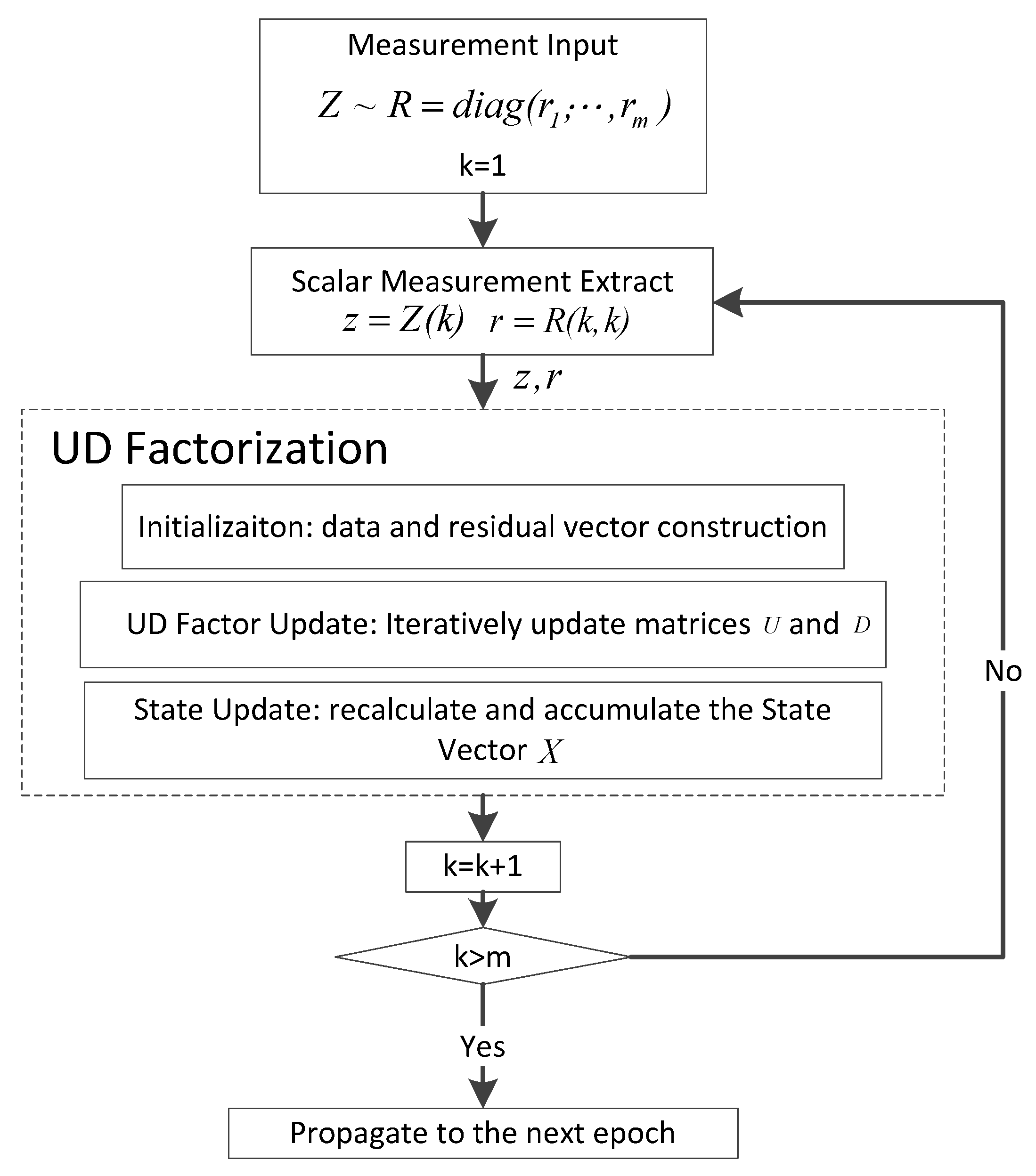
where , . As the differential operation is canceled in Equation (12), the recursion of avoids numerical instability [43]. The process of UD-KF is shown in Figure 1, and the specific implementation of UD factorization is given in Table 1 step by step.
As shown in Figure 1, the scalar element of R is sequentially imported, and the following superiorities can be drawn [44]: (1) X and K are implicitly obtained without an additional computational burden; (2) because 0 ≤ αj − 1/αj≤ 1 and is iteratively obtained by multiplication with its former values, the numeric accuracy is enhanced and cancellation-type errors are avoided [45]; and (3) computation efficiency is improved, as Z is proposed in a component-wise manner, and the updating of αj requires sequential multiplication and superposition of newly constructed f and v.
Figure 2 summarizes the flow of UD-KF, and the positioning solution is divided into the filtering stage and the fixing stage [46]. The filter is initialized by LS based on conventional DD measurements to form the VC matrix and weighting matrix of X at the first epoch [47]. Φ can be defined as an identity matrix without cycle slip. Q can be defined as a zero matrix. A real-time cycle slip detection strategy is applied for data preprocessing [48]. While cycle slip is detected on i-th satellite, adequately large process noise (1000 cycles is a reasonable empirical value) must be added to Qii to guarantee stability and sensitivity [8,49]. To verify the proposed UD-KF, KF and DD measurements (DD-KF) are simultaneously implemented to obtain the float solution [30]. The least-square ambiguity decorrelation adjustment (LAMBDA) is applied to fix ambiguities [50].
3. Results and Discussion
To explore the effect of the UD-KF, a zero-baseline test, a test with different stationary baselines, and a vehicular dynamic experiment were conducted utilizing single-frequency GPS data. All results were obtained through postprocessing performed on an Intel Core i7 2.30 GHz notebook PC with 16 GB RAM running Windows 10.
3.1. Zero-Baseline Test
A dataset with 30 s intervals and E = 15° collected by station CUT00 on 1 January 2021, at Curtin University, Australia was analyzed. As shown in Figure 3, two zero-baselines (CUT0-CUT2, CUT0-CUT3) were formed, as a common antenna (TRM 59,800.00 SCIS) connects to three receivers, CUT0(Trimble NETR9), CUT2(Trimble NETR9), and CUT3(JAVAD TRE_G3TH_8). Figure 4 depicts the available number of satellites and relative dilution of precision (RDOP) in the partial observation period. The average of visible satellites and RDOP were 8 and 0.7, respectively, indicating an ideal environment for relative positioning.
The positioning error on the east (E), north (N), and up (U) components is illustrated in Figure 5. A rapid convergence appeared as the preset Q was tuned at the initial stage. The RMS and STD for the positioning error are summarized in Table 2.
For UD-KF, the mean RMS of the ENU components for baselines CUT0-CUT2 and CUT0-CUT3 was (0.5 mm, 0.2 mm, 0.3 mm) and (0.3 mm, 0.6 mm, 0.5 mm). For DD-KF, the mean RMS of CUT0-CUT2 and CUT0-CUT3 was (3.5 mm, 1.0 mm, 1.8 mm) and (13.0 mm, 2.3 mm, 7.6 mm). The mean STD of UD-KF for CUT0-CUT2 and CUT0-CUT3 was (0.3 mm, 0.2 mm, 0.3 mm) and (0.3 mm, 0.5 mm, 0.5 mm), respectively, while the mean STD of DD-KF was (1.9 mm, 0.7 mm, 1.7 mm) and (6.2 mm, 1.6 mm, 6.2 mm). The results show that the UD-KF is more accurate than the DD-KF in all three directions.
A conclusion can also be drawn that UD-KF converges significantly faster than DD-KF. In the CUT0-CUT2 test, UD-KF quickly converged within 2 mm, while DD-KF failed to converge within 2 mm in the first ten hours. In the CUT0-CUT3 test, UD-KF converged after a short period of fluctuation, while DD-KF converged only after the 15th hour and retained a bias in the eastward direction. The reason CUT0-CUT2 achieved smaller RMS and STD than CUT0-CUT3 for both processing models is mainly due to the similarities and differences in receiver types used at both ends of different baselines.
As UD-KF limited position error to the millimeter level as expected, it is an effective substitute for DD-KF. Despite similar positioning accuracy obtained by both models, UD-KF performed better than conventional DD-KF [50].
3.2. Static Test
3.2.1. Position Accuracy Analysis
As shown in Figure 6, the GPS L1 datasets with E = 15° were collected by 7 GNSS CORS stations located in Hongkong during 00 h−01 h on 1 January 2021. Six baselines with various distances were used; the processing schemes are listed in Table 3.
As shown in Figure 7, the RMS and STD of position error on ENU for UD-KF and DD-KF were all within 10 cm, which implies they performed similarly. Table 4 provides corresponding statistics. Negative values represent performance degradation, while positive values represent an improvement.
UD-KF performed better for short baselines (HKSC-HKST/HKSC-HKLM/HKSC-HKOH/HKSC-HKPC). Taking HKSC-HKOH as an example, when a switch was made from DD-KF to UD-KF, the RMS of the 1 s interval dataset was improved by (+2.38 cm, +1.12 cm, +0.39 cm), while the RMS of the 5 s interval dataset was improved by (+1.7 cm, +1.45 cm, +0.69 cm). For HKSC-HKPC, the positioning accuracy was improved on E and U components, but a 0.7% degradation appeared on N. Similarities can also be found in HKSC-HKKT/HKSC-HKLM. It should be noted that the RMS and STD in the upwards direction of baseline HKSC-HKLM were twice as large as in the DD-KF scheme, indicating a larger residual assignment. A reasonable explanation is that UD-KF cannot only enhance the positioning accuracy but also redistribute the positioning residual in different directions.
For the longer baselines, the position accuracy of the 5 s interval dataset degraded by (−0.94 cm, −0.44 cm, −1.46 cm) for HKSC-HKKS and improved by (+2.2 cm, +3.026 cm, +0.93 cm) for HKSC-HKKT. The possible reason for this discrepancy is that although UD-KF benefits positioning accuracy by removing the correlation of the measurements, the ZD observation may still be affected by atmospheric errors that have not been eliminated equivalently [38]. As a consequence, UD-KF achieved better positioning accuracy without distance correlation.
3.2.2. Redundancy and Ambiguity Dilution of Precision (ADOP) Analysis
To provide sufficient test data, the 1 s interval dataset used in the former section is analyzed here. The filtering and ambiguity fixing efficiency are also analyzed.
In Equation (6), the matrix M1 has a rank deficit of n. This implies that to convert the unknown parameters of the rover to the relative parameters, we should set the coordinate parameters, ZD ambiguities, and clock error of the base receiver to zero. In Equation (7), the matrix M2 has a rank deficit of 1. This means that the SD ambiguities of the reference satellite should be set to zero to keep the parameters independent, and the other equivalent SD ambiguities can be converted to equivalent DD ambiguities. This means that the number of states that need to be estimated for UD-KF and DD-KF should be the same [1,51].
The computational efficiency is closely related to model redundancy. Higher redundancies mean higher data utilization. Here, the redundancy is expressed as the difference between observations and unknown states. Taking phase and code measurements of n satellites into account, according to Equations (6) and (7), the proof can be summarized as follows:
For UD-KF: The number of observation equations is: 4n. The number of the unknown parameters is 3 + (n − 1).
For DD-KF: The number of observation equations is 2(n − 1). The number of unknown parameters is 3 + (n − 1).
As a result, the redundancies for UD-KF and DD-KF are 3n − 2 and n − 4, respectively.
ADOP is introduced to evaluate the GNSS model strength for ambiguity resolution, and is defined as [52]:
where ν is the number of ambiguities to be estimated, |·| is the determinant operator, and is formed by design matrix and noise matrix:
According to Equations (13) and (14), the ADOP is determined by the satellite geometric distribution H and measurement noise R. Compared to DD-KF, UD-KF maintained superiority in the following two aspects: (1) the noise level of ZD measurements applied in UD-KF was not enlarged by difference operation, and (2) the higher redundancy of UD-KF can improve the geometric distribution.
Figure 8 shows the ADOP of each baseline with more than six satellites stably observed. An ADOP less than 1 cycle implies a good observation environment. For DD-KF, the ADOP showed a downward trend and converged near 0.4 cycles as time increased. For UD-KF, ADOP changed under different baselines with a consistent trend, rapidly dropping down and stably converging near 0.05 cycles. The ADOP performance of UD-KF was better than that of DD-KF. This is mainly because of the high data utilization and the lower noise level due to employing the equivalent ZD measurements.
3.2.3. Computation Efficiency Analysis
The time consumption of the filtering and fixing stage at each epoch is shown in Figure 9 and Figure 10, respectively. Here, the 1-h observation data with a 1 s sample rate was adopted (a total of 3600 epochs). The ‘Total Filter Time’ and ‘Total Fix Time’ were the time consumption at the ‘filter stage’ and ‘fix stage’ for the whole hour, respectively. The blue and red dots represent the calculation time of UD-KF and DD-KF, respectively. Although the time burden of filtering and fixing was on the order of milliseconds, UD-KF took significantly less time than DD-KF [53].
Table 5 gives the total time consumption for 3600 epochs of each baseline. The total filtering time was within 600 ms for UD-KF, with an average of 541.385 ms, while the filtering time was more than 700 ms, with an average of 818.26 ms, for DD-KF. The proposed strategy improved the computational efficiency, especially the time burden of HKSC-HKKT is reduced by 51.06%.
The total fixing time of UD-KF was less than 3100 ms, for which the minimum was 2729.49 ms and the maximum was 3037.49 ms. However, the minimum of DD-KF was 3189.85 ms, and the maximum was 3715.58 ms. UD-KF achieved efficiency improvement of (18.25%, 21.95%, 24.91%, 12.10%, 15.82%, 16.59%) on each baseline. Additionally, the success rate of the ambiguity fixing of UD-KF and DD-KF remained at a high level, although more ambiguities needed to be fixed by UD-KF.
3.3. Kinematic Test
The dynamic efficiency and accuracy of the UD-KF were statistically analyzed by conducting a test in the urban environment of Wuhan, China, on 29 July 2021, from 6:04 to 8:55 UTC, along the trajectory shown in Figure 11.
A temporary base station was set up nearby the terminal, whose coordinate was determined through PPP with 2 h static data. The rover with a 1 Hz output rate was mounted on the roof of the experimental vehicle. During the test, 6–10 satellites were stably available. Furthermore, the postprocessing results of DD-KF were treated as reference coordinates. If the three-dimensional error of positioning was less than 20 cm, this epoch was regarded as a successful positioning [54].
Figure 12a shows the resulting trajectory in an open-sky environment. The vehicle motion will change due to acceleration and deceleration. Figure 12b shows the result in the street scene, in which the signal was seriously blocked by buildings and vegetation. The yellow dots and red dots denote the trajectory of UD-KF and DD-KF, respectively. The positioning difference between the two models is shown in Figure 13. Apart from a few epochs, the difference was less than 20 cm for the U component and 10 cm for the E and N component. The interrelating RMS and STD in ENU were (1.14 cm, 1.06 cm, 1.48 cm) and (1.12 cm, 1.05 cm, 1.48 cm), respectively. This implies that UD-KF maintained consistency with DD-KF under dynamic conditions. The calculation time burden of UD-KF and DD-KF for filtering was (1063.51 ms, 1424.24 ms) and (2969.69 ms, 3413.47 ms) for fixing ambiguities, respectively, an improvement of (25.33%, 13.00%).
A change in satellites leads to the change of model redundancy, which can cause different calculation burdens. We further evaluated whether the UD-KF could provide robust efficiency improvement when satellites change; the top and middle of Figure 14 show the results of (DD-KF time burden minus UD-KF time burden) at each epoch for different stages. The corresponding number of satellites is shown at the bottom of Figure 14.
There were seven to nine satellites that could be observed by the base receiver and rover receiver separately, but common-view satellites vary greatly due to obstacles and blockage. The position of the rover relies entirely on the time update of KF when less than four satellites are available.
The positive values of the time difference in Figure 14 (top and middle) imply that UD-KF experienced a smaller computation burden at each epoch than DD-KF. At each epoch, the time consumption was reduced on average by 0.11 ms at the filtering stage and 0.13 ms at the fixing stage. Meanwhile, the UD-KF was insensitive to satellite change, remaining stable during the time difference of each stage while the number of satellites changed drastically. It can be inferred that UD-KF can steadily improve efficiency and avoid the impact on the environment, which further shows its robustness in the urban environment [55].
4. Conclusions
In order to tackle the dilemma of a restricted processing capacity of GNSS IoT devices, in this contribution we proposed a new and efficient equivalent ZD algorithm for RTK. First of all, conventional DD measurements were decorrelated to equivalent ZD measurements by the equivalent principle. Additionally, the sequential strategy for RTK was constructed by the UD factorization implementation. The most outstanding feature of UD-KF is that it has a rigorous model that can enhance numeric stability and efficiency with high data utilization and availability. The results show that the proposed method can achieve faster convergence and higher positioning accuracy efficiently compared with the conventional DD-KF. The following conclusions were obtained:
- (1)
- For the zero-baseline test, UD-KF achieved a better positioning accuracy than DD-KF, which validates the reliability and feasibility of the new proposed algorithm. If the same type of receivers is used at both ends of the baseline, UD-KF can reduce the RMS of the position error by 86% on E, 80% on N, and 83% on U, as compared to the conventional DD-KF.
- (2)
- For the static test, UD-KF achieved better position accuracy for short baselines. The increase in baseline distance does not affect the positioning performance of UD-KF. The average performance improvement of RMS for six baselines was 69% on E and 27% on N, and more errors occurred on the U component. The computational efficiency was improved by 25–50% at the filtering stage and 15–25% at the fixing stage.
- (3)
- For the dynamic test, the robustness of UD-KF was verified by the reduction in time consumption, which kept stable when satellites in view changed dramatically. The UD-KF achieved an accurate position in typical urban environments and accelerated the filtering and fixing process by (0.11 ms, 0.13 ms), respectively, for each epoch.
Our future work will extend the proposed method to multifrequency and multi-GNSS positioning, considering the computational efficiency and exploring its application in the field of deep combination with vector tracking to improve the precision and reliability of dynamic positioning in the urban environment.
Author Contributions
Conceptualization, J.L.; methodology, J.L.; software, J.L., T.L. and B.Z.; investigation, B.Z., Y.J., M.S. and Y.H.; data curation, J.L. and W.N.; writing—original draft preparation, J.L.; writing—review and editing, B.Z., T.L., W.N. and G.X.; supervision, Y.J. and G.X. All authors have read and agreed to the published version of the manuscript.
Funding
This study was supported by the Shenzhen Science and Technology Program (Grant No. KQTD20180410161218820); the Opening Project of Guangxi Wireless Broadband Communication and Signal Processing Key Laboratory (No. GXKL06200217); the Guangdong Basic and Applied Basic Research Foundation (No: 2021A1515012600); the National Nature Science Foundation of China (No. 42004012); the Natural Science Foundation of Shandong Province (No. ZR2020QD048); the State Key Laboratory of Geodesy and Earth’s Dynamics, Innovation Academy for Precision Measurement Science and Technology, Chinese Academy of Sciences (No. SKLGED2021-3-4), and the State Key Laboratory of Geo-Information Engineering (No. SKLGIE2019-Z-2-2).
Data Availability Statement
The authors are grateful to the Curtin GNSS Research Center of Curtin University and the Survey and Mapping Office Lands Department of Hong Kong for publicly sharing their GNSS data.
Acknowledgments
We are grateful to the anonymous reviewers and editors for their helpful and constructive suggestions, which significantly improved the paper quality. Figure 6 was edited using the public domain Generic Mapping Tools GMT, and Figure 11 and Figure 12 were edited using Google Earth, which is also acknowledged.
Conflicts of Interest
The authors declare no conflict of interest.
References
- Wang, J.; Xu, T.; Nie, W.; Xu, G. A Simplified Processing Algorithm for Multi-baseline RTK Positioning in Urban Environments. Measurement 2021, 179, 109446. [Google Scholar] [CrossRef]
- Liu, T.; Xu, T.; Nie, W.; Li, N. Optimal Independent Baseline Searching for Global GNSS Networks. J. Surv. Eng. 2020, 147, 05020010. [Google Scholar] [CrossRef]
- Krasuski, K.; Savchuk, S. Determination of the Precise Coordinates of the GPS Reference Station in of a GBAS System in the Air Transport. Komunikacie 2020, 22, 11–18. [Google Scholar] [CrossRef]
- Liu, T.; Yu, Z.; Ding, Z.; Nie, W.; Xu, G. Observation of Ionospheric Gravity Waves Introduced by Thunderstorms in Low Latitudes China by GNSS. Remote Sens. 2021, 13, 4131. [Google Scholar] [CrossRef]
- Cetin, S.; Aydin, C.; Dogan, U. Comparing GPS positioning errors derived from GAMIT/GLOBK and Bernese GNSS software packages: A case study in CORS-TR in Turkey. Surv. Rev. 2019, 51, 533–543. [Google Scholar] [CrossRef]
- Mao, X.; Arnold, D.; Girardin, V.; Villiger, A.; Jäggi, A. Dynamic GPS-based LEO orbit determination with 1 cm precision using the Bernese GNSS Software. Adv. Space Res. 2021, 67, 788–805. [Google Scholar] [CrossRef]
- Xu, P.; Du, F.; Shu, Y.; Zhang, H.; Shi, Y. Regularized reconstruction of peak ground velocity and acceleration from very high-rate GNSS precise point positioning with applications to the 2013 Lushan Mw6.6 earthquake. J. Geod. 2021, 95, 1–22. [Google Scholar] [CrossRef]
- Takasu, T.; Yasuda, A. Development of the Low-Cost RTK-GPS Receiver with an Open Source Program Package RTKLIB; International Symposium on Gps/gnss: Jeju, Korea, 2009; Volume 1, pp. 1–6. [Google Scholar]
- Jiang, X.; Gu, S.; Li, P.; Ge, M.; Schuh, H. A Decentralized Processing Schema for Efficient and Robust Real-time Multi-GNSS Satellite Clock Estimation. Remote Sens. 2019, 11, 2595. [Google Scholar] [CrossRef] [Green Version]
- Berkay, B.; Metin, N. PPPH: A MATLAB-based software for multi-GNSS precise point positioning analysis. GPS Solut. 2018, 22, 113. [Google Scholar]
- Tondaś, D.; Kapłon, J.; Rohm, W. Ultra-fast near real-time estimation of troposphere parameters and coordinates from GPS data. Measurement 2020, 162, 107849. [Google Scholar] [CrossRef]
- Aragon-Angel, A.; Garcia, A.R.; Arcediano-Garrido, E.; Ibáñez, D. Galileo Ionospheric correction algorithm integration into the open-source GNSS Laboratory Tool Suite (gLAB). Remote Sens. 2021, 13, 191. [Google Scholar] [CrossRef]
- Li, Y. Analysis of GAMIT/GLOBK in high-precision GNSS data processing for crustal deformation. Earthq. Res. Adv. 2021, 1, 100028. [Google Scholar] [CrossRef]
- Lyros, E.; Kostelecky, J.; Plicka, V.; Vratislav, F.; Sokos, E.; Nikolakopoulos, K. Detection of tectonic and crustal deformation using GNSS data processing: The case of ppgnet. Civ. Eng. J. 2021, 7, 14–23. [Google Scholar] [CrossRef]
- Jiang, C.; Xu, T.; Du, Y.; Sun, Z.; Xu, G. A parallel equivalence algorithm based on MPI for GNSS data processing. J. Spat. Sci. 2021, 66, 513–532. [Google Scholar] [CrossRef]
- Li, L.; Lu, Z.; Chen, Z.; Cui, Y.; Sun, D.; Wang, Y.; Kuang, Y.; Wang, F. GNSSer: Objected-oriented and design pattern-based software for GNSS data parallel processing. J. Spat. Sci. 2021, 66, 27–47. [Google Scholar] [CrossRef]
- Xu, G.; Xu, Y. Applications of GPS theory and algorithms. In GPS; Springer: Berlin/Heidelberg, Germany, 2016. [Google Scholar]
- Szot, T.; Specht, C.; Specht, M.; Dabrowski, P.S. Comparative analysis of positioning accuracy of Samsung Galaxy smartphones in stationary measurements. PLoS ONE 2019, 14, e0215562. [Google Scholar] [CrossRef]
- Stateczny, A.; Kazimierski, W.; Burdziakowski, P.; Motyl, W.; Wisniewska, M. Shore Construction Detection by Automotive Radar for the Needs of Autonomous Surface Vehicle Navigation. ISPRS Int. J. Geo-Inf. 2019, 8, 80. [Google Scholar] [CrossRef] [Green Version]
- Lucas-Sabola, V.; Seco-Granados, G.; López-Salcedo, J.A.; García-Molina, J.A.; European Space Agency. GNSS IoT Positioning From Conventional Sensors to a Cloud-Based Solution. Inside GNSS 2018, 13, 53–62. [Google Scholar]
- Mayer, P.; Magno, M.; Berger, A.; Benini, L. RTK-LoRa: High-Precision, Long-Range, and Energy-Efficient Localization for Mobile IoT Devices. IEEE Trans. Instrum. Meas. 2020, 70, 1–11. [Google Scholar] [CrossRef]
- Duan, B.; Wang, J. Factorization Method for GNSS Parameter Estimation. In Proceedings of the International Symposium on Satellite Mapping Technology and Application (ISSMTA2013), Nanjing, China, 6–8 November 2013. [Google Scholar]
- Zarchan, P. Progress in Astronautics and Aeronautics: Fundamentals of Kalman Filtering: A Practical Approach; AIAA: Reston, VI, USA, 2005; Volume 208. [Google Scholar]
- Vaclavovic, P.; Dousa, J. Backward smoothing for precise GNSS applications. Adv. Space Res. 2015, 56, 1627–1634. [Google Scholar] [CrossRef]
- Evangelidis, A.; Parker, D. Quantitative verification of numerical stability for Kalman filters. In International Symposium on Formal Methods; Springer: Berlin/Heidelberg, Germany, 2019. [Google Scholar]
- Wang, G.; Xue, R.; Zhao, J. Switching criterion for sub-and super-Gaussian additive noise in adaptive filtering. Signal Proc. 2018, 150, 166–170. [Google Scholar] [CrossRef]
- Wang, G.; Zhang, Y.; Wang, X. Maximum correntropy Rauch–Tung–Striebel smoother for nonlinear and non-Gaussian systems. IEEE Trans. Autom. Control 2020, 66, 1270–1277. [Google Scholar] [CrossRef]
- Kulikova, M.V. Factored-form Kalman-like implementations under maximum correntropy criterion. Signal Proc. 2019, 160, 328–338. [Google Scholar] [CrossRef]
- Cilden-Guler, D.; Hajiyev, C. SVD-aided EKF attitude estimation with UD factorized measurement noise covariance. Asian J. Control 2019, 21, 1423–1432. [Google Scholar] [CrossRef]
- Realini, E.; Reguzzoni, M. goGPS: Open source software for enhancing the accuracy of low-cost receivers by single-frequency relative kinematic positioning. Meas. Sci. Technol. 2013, 24, 115010. [Google Scholar] [CrossRef]
- Miao, W.; Li, B.; Zhang, Z.; Zhang, X. Combined BeiDou-2 and BeiDou-3 instantaneous RTK positioning: Stochastic modeling and positioning performance assessment. J. Spat. Sci. 2020, 65, 7–24. [Google Scholar] [CrossRef]
- Borko, A.; Even-Tzur, G. Stochastic model reliability in GNSS baseline solution. J. Geod. 2021, 95. [Google Scholar] [CrossRef]
- Jiang, Y.; Gao, Y.; Zhou, P.; Gao, Y.; Huang, G. Real-time cascading PPP-WAR based on Kalman filter considering time-correlation. J. Geod. 2021, 95, 1–15. [Google Scholar] [CrossRef]
- Liu, M.; Chang, G. Numerically and statistically stable Kalman filter for INS/GNSS integration. Proc. Inst. Mech. Eng. Part G J. Aerosp. Eng. 2016, 230, 321–332. [Google Scholar] [CrossRef]
- Cao, X.; Li, J.; Zhang, S.; Pan, L.; Kuang, K. Performance assessment of uncombined precise point positioning using Multi-GNSS real-time streams: Computational efficiency and RTS interruption. Adv. Space Res. 2018, 62, 3133–3147. [Google Scholar] [CrossRef]
- Khamseh, H.B.; Ghorbani, S.; Janabi-Sharifi, F. Unscented Kalman filter state estimation for manipulating unmanned aerial vehicles. Aerosp. Sci. Technol. 2019, 92, 446–463. [Google Scholar] [CrossRef]
- Dong, Y.; Wang, D.; Zhang, L.; Li, Q.; Wu, J. Tightly coupled GNSS/INS integration with robust sequential kalman filter for accurate vehicular navigation. Sensors 2020, 20, 561. [Google Scholar] [CrossRef] [PubMed] [Green Version]
- Tu, R.; Lu, C.; Zhang, P.; Zhang, R.; Liu, J.; Lu, X. The study of BDS RTK algorithm based on zero-combined observations and ionosphere constraints. Adv. Space Res. 2019, 63, 2687–2695. [Google Scholar] [CrossRef]
- Schaffrin, B.; Grafarend, E. Generating classes of equivalent linear models by nuisance parameter. Manuscr. Geod. 1986, 11, 262–271. [Google Scholar]
- Wang, J.; Xu, T.; Nie, W.; Xu, G. GPS/BDS RTK Positioning Based on Equivalence Principle Using Multiple Reference Stations. Remote Sens. 2020, 12, 3178. [Google Scholar] [CrossRef]
- Xu, Y. GNSS Precise Point Positioning with Application of the Equivalence Principle; Technische Universitaet Berlin (Germany): Berlin, Germany, 2016. [Google Scholar]
- Yongyuan, Q.; Hongyue, Z.; Shuhua, W. Kalman Filter and Principle of Integrated Navigation; The Publishing Company of Northwestern Polytechnical University: Xi’an, China, 2015; Volume 182, p. 187. [Google Scholar]
- Kulikova, M.V.; Tsyganova, J.V. The UD-based approach for designing pairwise Kalman filtering algorithms. IFAC-Pap. 2017, 50, 1619–1624. [Google Scholar] [CrossRef]
- Bierman, G.J. Measurement updating using the UD factorization. Automatica 1976, 12, 375–382. [Google Scholar] [CrossRef]
- Wang, G.; Chen, B.; Yang, X.; Peng, B.; Feng, Z. Numerically stable minimum error entropy Kalman filter. Signal Proc. 2021, 181, 107914. [Google Scholar] [CrossRef]
- Pang, C.; Long, F.; Liang, J.; Chen, H.; Yuan, M. Algorithm of rapid integer ambiguity resolution for single frequency GPS receivers based on improved UDVT decomposition. Acta Aeronaut. Astronaut. Sin. 2012, 33, 102–109. [Google Scholar]
- Xie, G. Principles of GPS and Receiver Design; Publishing House of Electronics Industry: Beijing, China, 2009; Volume 7, pp. 61–63. [Google Scholar]
- Li, B. Single-frequency GNSS cycle slip estimation with positional polynomial constraint. J. Geod. 2019, 93, 1781–1803. [Google Scholar] [CrossRef]
- Gelen, A.G.; Atasoy, A. A New Method for Kalman Filter Tuning. In Proceedings of the 2018 International Conference on Artificial Intelligence and Data Processing (IDAP), Malatya, Turkey, 28–30 September 2018; IEEE: Piscataway, NJ, USA, 2018. [Google Scholar]
- Zhao, S.; Cui, X.; Guan, F.; Lu, M. A Kalman filter-based short baseline RTK algorithm for single-frequency combination of GPS and BDS. Sensors 2014, 14, 15415–15433. [Google Scholar] [CrossRef] [PubMed]
- Shen, Y.; Xu, G. Simplified equivalent representation of GPS observation equations. GPS Solut. 2008, 12, 99–108. [Google Scholar] [CrossRef]
- Teunissen, P.J.; Odijk, D. Ambiguity dilution of precision: Definition, properties and application. In Proceedings of the 10th International Technical Meeting of the Satellite Division of The Institute of Navigation (ION GPS 1997), Kansas, MO, USA, 16–19 September 1997. [Google Scholar]
- Chang, G.; Chen, C.; Zhang, Q.; Zhang, S. Variational Bayesian adaptation of process noise covariance matrix in Kalman filtering. J. Frankl. Inst. 2021, 358, 3980–3993. [Google Scholar] [CrossRef]
- Furones, A.M.; Julián, A.B.A.; Dimas-Pages, A.; Cos-Gayón, F. Computational time reduction for sequential batch solutions in GNSS precise point positioning technique. Comput. Geosci. 2017, 105, 34–42. [Google Scholar] [CrossRef] [Green Version]
- Kulikova, M.V. Sequential maximum correntropy Kalman filtering. Asian J. Control 2020, 22, 25–33. [Google Scholar] [CrossRef]
Figure 1.
Flow chart of UD-KF Strategy.

Figure 2.
Flow chart of UD-Factorization implementation for KF based on equivalent principle.

Figure 3.
(a) Location of station CUT00; red lines represent the spacing distance from other stations; (b) manufacturer and type for three receivers (CUT0, CUT2, and CUT3). (http://saegnss2.curtin.edu/ldc/CU-GNSS-receivers-setup.pdf, accessed on 1 December 2021).
Figure 3.
(a) Location of station CUT00; red lines represent the spacing distance from other stations; (b) manufacturer and type for three receivers (CUT0, CUT2, and CUT3). (http://saegnss2.curtin.edu/ldc/CU-GNSS-receivers-setup.pdf, accessed on 1 December 2021).

Figure 4.
RODP and available satellites of station CUT00.

Figure 5.
ENU position error for zero-baseline test of CUT00.

Figure 6.
The information of 6 baselines for the static test.

Figure 7.
RMS and STD for different baselines.

Figure 8.
ADOP of UD-KF and DD-KF.

Figure 9.
Filter computation efficiency.

Figure 10.
Fix computation efficiency.

Figure 11.
(a) The trajectory of the kinematic test; (b) sky plot of the kinematic test.

Figure 12.
The positioning result for UD-KF (a) and DD-KF (b) for different scenes.

Figure 13.
Position result difference for ENU for the kinematic test.

Figure 14.
Filter and fix time difference and the corresponding satellite number.


Table 1.
A stepwise implementation of UD factorization.
| Step | Stage | Implementation |
|---|---|---|
| 1 | Initialization | |
| 2 | U-D factor Update | for j = 2:n for i = 1: j − 1 , end end |
| 3 | State Update | for j = 1:g end |
Table 2.
The RMS and STD of the positioning error.
| Processing Model | CUT0-CUT2 | CUT0-CUT3 | |||||
|---|---|---|---|---|---|---|---|
| E | N | U | E | N | U | ||
| RMS (mm) | UD-KF | 0.5 | 0.2 | 0.3 | 0.3 | 0.6 | 0.5 |
| DD-KF | 3.5 | 1.0 | 1.8 | 13.0 | 2.3 | 7.6 | |
| STD (mm) | UD-KF | 0.3 | 0.2 | 0.3 | 0.3 | 0.5 | 0.5 |
| DD-KF | 1.9 | 0.7 | 1.7 | 6.2 | 1.6 | 6.2 | |
Table 3.
The processing schemes for different baselines.
| No. | Baseline | Distance (km) | Interval | Processing Model | |
|---|---|---|---|---|---|
| Base | Rover | ||||
| 1 | HKKT | HKSC | 15.613 | 1 s, 5 s | UD-KF, DD-KF |
| 2 | HKKS | HKSC | 18.303 | 1 s, 5 s | UD-KF, DD-KF |
| 3 | HKLM | HKSC | 11.634 | 1 s, 5 s | UD-KF, DD-KF |
| 4 | HKOH | HKSC | 12.211 | 1 s, 5 s | UD-KF, DD-KF |
| 5 | HKPC | HKSC | 11.418 | 1 s, 5 s | UD-KF, DD-KF |
| 6 | HKST | HKSC | 9.232 | 1 s, 5 s | UD-KF, DD-KF |
Table 4.
RMS and STD improvement rate on ENU.
| Baseline | Interval | E | N | U | |||||||
|---|---|---|---|---|---|---|---|---|---|---|---|
| UD | DD | Improvement | UD | DD | Improvement | UD | DD | Improvement | |||
| RMSE (cm) | HKSC-HKKT | 1 s | 2.73 | 6.02 | 54.65% | 2.34 | 2.82 | 17.02% | 8.07 | 4.54 | −77.75% |
| 5 s | 1.19 | 3.39 | 64.90% | 1.314 | 4.34 | 69.72% | 2.61 | 3.54 | 26.27% | ||
| HKSC-HKKS | 1 s | 0.67 | 0.74 | 9.46% | 0.88 | 1.87 | 52.94% | 2.43 | 1.251 | −94.24% | |
| 5 s | 1.69 | 0.75 | −125.33% | 2.09 | 1.65 | −26.67% | 2.70 | 1.24 | −117.74% | ||
| HKSC-HKLM | 1 s | 1.14 | 3.50 | 67.43% | 0.93 | 0.81 | −14.81% | 2.89 | 1.24 | −133.06% | |
| 5 s | 1.07 | 2.92 | 63.36% | 1.06 | 1.01 | −4.95% | 2.80 | 1.12 | −150% | ||
| HKSC-HKOH | 1 s | 0.69 | 3.07 | 77.52% | 1.07 | 2.19 | 51.14% | 2.40 | 2.79 | 13.98% | |
| 5 s | 0.65 | 2.35 | 72.34% | 0.78 | 2.23 | 65.02% | 1.75 | 2.44 | 28.28% | ||
| HKSC-HKPC | 1 s | 1.12 | 3.83 | 70.76% | 1.37 | 1.36 | −0.73% | 3.51 | 3.95 | 11.14% | |
| 5 s | 1.01 | 4.72 | 78.60% | 1.19 | 1.09 | −9.17% | 3.36 | 4.39 | 23.46% | ||
| HKSC-HKST | 1 s | 1.15 | 0.91 | −26.37% | 1.14 | 0.89 | −28.09% | 4.012 | 6.08 | 34.01% | |
| 5 s | 1.21 | 1.18 | −2.54% | 1.43 | 0.71 | −101.41% | 4.16 | 6.58 | 36.78% | ||
| STD (cm) | HKSC-HKKT | 1 s | 2.61 | 4.83 | 45.96% | 2.28 | 2.52 | 9.52% | 7.97 | 4.35 | −83.22% |
| 5 s | 0.96 | 2.52 | 61.90% | 1.01 | 4.32 | 76.62% | 2.58 | 3.34 | 22.75% | ||
| HKSC-HKKS | 1 s | 0.64 | 0.54 | −18.52% | 0.82 | 1.51 | 45.70% | 2.43 | 0.74 | −228.38% | |
| 5 s | 1.69 | 0.49 | −244.90% | 1.60 | 1.12 | −42.86 | 2.70 | 0.77 | −250.65% | ||
| HKSC-HKLM | 1 s | 1.14 | 1.72 | 33.72% | 0.84 | 0.77 | −9.09% | 2.82 | 0.73 | −286.30% | |
| 5 s | 1.05 | 1.37 | 23.36% | 0.96 | 0.93 | −3.23% | 2.76 | 0.71 | −288.73% | ||
| HKSC-HKOH | 1 s | 0.65 | 1.48 | 56.08% | 0.94 | 1.79 | 47.49% | 2.25 | 1.12 | −100.89% | |
| 5 s | 0.65 | 1.15 | 43.48% | 0.72 | 1.77 | 59.32% | 1.75 | 1.66 | −5.42% | ||
| HKSC-HKPC | 1 s | 1.04 | 3.53 | 70.54% | 1.35 | 1.07 | −26.17% | 3.45 | 3.812 | 9.50% | |
| 5 s | 1.01 | 3.88 | 73.97% | 1.18 | 0.85 | −38.82% | 3.36 | 4.09 | 17.85% | ||
| HKSC-HKST | 1 s | 1.13 | 0.90 | −25.56% | 1.099 | 0.88 | −24.89% | 3.94 | 4.611 | 14.55% | |
| 5 s | 1.06 | 1.00 | −6.00% | 1.42 | 0.69 | −105.80% | 4.06 | 4.54 | 10.57% | ||
Table 5.
Total time consumption statistics.
| Baseline | Total Filer Time (ms) | Improvement | Total Fix Time(ms) | Fix Rate | Improvement | |||
|---|---|---|---|---|---|---|---|---|
| UD-KF | DD-KF | UD-KF | DD-KF | UD-KF | DD-KF | |||
| HKSC-HKST | 599.37 | 844.83 | 29.05% | 3037.49 | 3715.58 | 98.47% | 100% | 18.25% |
| HKSC-HKKT | 525.31 | 1073.34 | 51.06% | 2801.20 | 3589.02 | 93.14% | 94.42% | 21.95% |
| HKSC-HKPC | 518.57 | 777.03 | 33.26% | 2729.49 | 3634.99 | 98.25% | 98.92% | 24.91% |
| HKSC-HKLM | 541.10 | 741.99 | 27.07% | 2803.85 | 3189.85 | 83.58% | 84.47% | 12.10% |
| HKSC-HKOH | 535.73 | 746.97 | 28.28% | 2858.32 | 3395.42 | 98.56% | 100% | 15.82% |
| HKSC-HKKS | 528.23 | 725.42 | 27.18% | 2798.22 | 3354.70 | 98.39% | 100% | 16.59% |
Publisher’s Note: MDPI stays neutral with regard to jurisdictional claims in published maps and institutional affiliations. |
© 2022 by the authors. Licensee MDPI, Basel, Switzerland. This article is an open access article distributed under the terms and conditions of the Creative Commons Attribution (CC BY) license (https://creativecommons.org/licenses/by/4.0/).
Share and Cite
MDPI and ACS Style
Liu, J.; Zhang, B.; Liu, T.; Xu, G.; Ji, Y.; Sun, M.; Nie, W.; He, Y. An Efficient UD Factorization Implementation of Kalman Filter for RTK Based on Equivalent Principle. Remote Sens. 2022, 14, 967. https://doi.org/10.3390/rs14040967
AMA Style
Liu J, Zhang B, Liu T, Xu G, Ji Y, Sun M, Nie W, He Y. An Efficient UD Factorization Implementation of Kalman Filter for RTK Based on Equivalent Principle. Remote Sensing. 2022; 14(4):967. https://doi.org/10.3390/rs14040967
Chicago/Turabian StyleLiu, Jian, Bing Zhang, Tong Liu, Guochang Xu, Yuanfa Ji, Mengfei Sun, Wenfeng Nie, and Yufang He. 2022. "An Efficient UD Factorization Implementation of Kalman Filter for RTK Based on Equivalent Principle" Remote Sensing 14, no. 4: 967. https://doi.org/10.3390/rs14040967
Note that from the first issue of 2016, this journal uses article numbers instead of page numbers. See further details here.