Article

Unsupervised Optical Classification of the Seabed Color in Shallow Oligotrophic Waters from Sentinel-2 Images: A Case Study in the Voh-Koné-Pouembout Lagoon (New Caledonia)

1
Interdisciplinary Laboratory for Research in Education, EA 7483, University of New Caledonia, Avenue James Cook, Noumea 98800, New Caledonia
2
Mediterranean Institute of Oceanography (MIO), Aix-Marseille Université, CNRS/INSU, Université de Toulon, IRD, UM 110, 13288 Marseille, France
3
Centre IRD Noumea, Noumea 98848, New Caledonia
4
Institut de Minéralogie, de Physique des Matériaux et de Cosmochimie (IMPMC), ERL IRD 206, UMR CNRS 7590, MNHN, Sorbonne Université, 75005 Paris, France
*
Author to whom correspondence should be addressed.
Remote Sens. 2022, 14(4), 836; https://doi.org/10.3390/rs14040836
Submission received: 22 December 2021 / Revised: 31 January 2022 / Accepted: 7 February 2022 / Published: 10 February 2022
(This article belongs to the Special Issue Satellite Mapping and Monitoring of the Coastal Zone)

Abstract

:
Monitoring chlorophyll-a concentration or turbidity is crucial for understanding and managing oligo- to mesotrophic coastal waters quality. However, mapping bio-optical components from space in such shallow settings remains challenging because of the strong interference of the complex bathymetry and various seabed colors. Correcting the total satellite reflectance signal from the seabed reflectance in ocean color with high resolution sensors is promising. This article shows how unsupervised clustering approaches can be applied to Sentinel-2 images to classify seabed colors in shallow waters of a tropical oligotrophic lagoon in New Caledonia. Data processing included Lyzenga correction for estimating the water column reflectance, optical spectra standardization for attenuating water absorption effects and clustering using the unsupervised k-means method. This methodological approach was applied on the 497, 560, 664 and 704 nm optical bands of the selected Sentinel-2 image. When applied on non-standardized data, our unsupervised classification retrieved three seafloor clusters, whereas five seafloor clusters could be retrieved using standardized data. For each of these two trials, the computed membership values explained more than 75% of the inertia in each Sentinel-2 wavelength band used for the clustering. However, the accuracy of the method was slightly improved when applied on standardized data. Confusion index mapping of the unsupervised clustering retrieved from these data emphasized the relevance and robustness of our methodological approach. Such an approach for seabed colors classification in optically complex shallow settings will be particularly helpful to improve remote sensing of biogeochemical indicators such as chlorophyll-a concentration and turbidity in fragile coastal environments.

Graphical Abstract

1. Introduction

In the context of global environmental changes, there is still a tremendous need for indicators of oceanic coastal vulnerability in shallow waters of tropical lagoons, due to the economic importance of these areas [1,2,3]. A high variety of bio-optical and biogeochemical parameters can be derived [4,5] from empirical or semi-analytical algorithms for environmental monitoring by ocean color satellite imagery [6]. In the lagoon of New Caledonia, previous studies demonstrated the capacity of satellite-based data to estimate turbidity or chlorophyll-a concentration for waters deeper than 20 m [7,8]. However, similar approaches for oligotrophic shallow waters failed because of the strong influence of the seabed type on satellite reflectance [9,10]. In such coastal settings, recent studies using Support Vector Machine (SVM) relying on the introduction of environmental variables such as bathymetry and seabed color approach were successfully employed to remotely assess chlorophyll-a concentration [11] and turbidity [12]. Although bathymetry is an environmental variable easily accessible from satellite images, remote mapping of seabed color is more challenging. Seabed reflectance determination in shallow coastal waters is usually based on model inversion equations from forward models for reflectance (HydroLight-EcoLight) [13] or other semi-analytical models using look-up tables (LUT) for water column optical properties at different depths [14]. As an illustration, field estimation of the water attenuation coefficient in the Southern lagoon of New Caledonia allowed to map the bathymetry from a clear MERIS image [15], while supervised clustering helped to classify the seabed into three categories (white sand, grey sand and mud) [16]. However, such supervised clustering approaches rely on the availability of field data to be compared with computed parameters. In situations where such field data are missing, unsupervised classification might represent an option, as suggested by recent studies that successfully used this approach with side-scan sonar imagery and multibeam bathymetry data [17] or acoustic backscattering imagery generated from a multibeam sounder [18]. The very low confusion indices (CI) obtained in these studies emphasizes the great potential of unsupervised classification to unravel seabed classification in shallow oligotrophic coastal waters based on satellite images.
The objective of this study was to apply unsupervised classification of seabed reflectance on a selected area from the Northern lagoon of New Caledonia that is characterized by shallow oligotrophic waters. Our leading hypothesis was that the various seabed colors at the investigated area could be discriminated based on their specific spectral signatures, knowing the bathymetry. The processed spectral signatures were extracted from a Sentinel-2 multispectral image. Such high-resolution sensors were already used to map water quality [19], turbidity [20] or bathymetry and coral reefs in tropical environments similar to the one investigated in this study [21,22]. In the present study, the processing steps used to cluster the seabed spectral reflectance at the investigated area are described and the strengths and shortcomings of the approach are discussed. This approach is expected to be widely reproducible whatever the in situ data available, provided the environmental context is similar (i.e., oligotrophic shallow coastal waters).

2. Materials and Methods

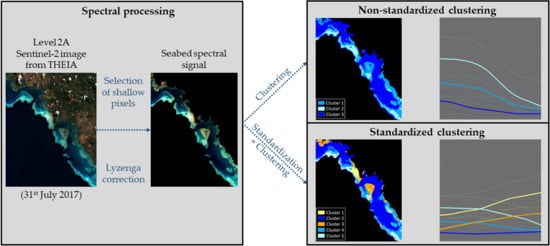
2.1. General Conception of the Study

Figure 1 provides an overview of the process used for conducting this study. The aim of this study was to cluster the seabed spectral signal in the Voh-Koné-Pouembout (VKP) area of the North-Western lagoon from New Caledonia. For that purpose, a Sentinel-2 image was selected and the Lyzenga correction was applied in order to get the seabed spectral signal by withdrawing the water column contribution [15,16,23]. Then, an unsupervised clustering of the corrected pixels of the image was performed in order to cluster pixels with similar seabed spectral signal (i.e., hereafter referred to as “non-standardized clustering”). In addition, we also attempted to cluster the pixels of the image after standardization of the spectral signal (i.e., hereafter referred to as “standardized clustering”). Finally, the pixels clustered with both the “non-standardized clustering” and “standardized clustering” approaches were used to build seabed color maps that could further be implemented in the satellite-based model using unsupervised classification to depict the spatial distribution of environmental parameters in the investigated shallow coastal waters.

2.2. Study Area

The Voh-Kone-Pouembout (VKP) lagoon is a small part (West Coast, Northern Province) of the New Caledonia lagoon, a south Pacific archipelago located between 162–169° E longitude and 19–23° S latitude (Figure 2A) which covers a total surface of 20,000 km2 and holds a large diversity of habitats (Figure 2B). Considering the bathymetric data extracted from the 100 m resolution file of the New Caledonia administration database [24], depth in the VKP lagoon is usually less than 5 m (around 70% of the lagoon surface; Figure 2C). However, it can exceed 30 m in passes and around, with an average value of around 20 m (Figure 2C). During a 2010–2015 environmental survey performed at 54 stations in the VKP lagoon, about 85% of in situ measurements revealed turbidity values below 2.0 NTU, and more than 70% values were below 1.0 NTU. These values are in agreement with the known oligotrophic characteristics of the lagoon waters in New Caledonia [7,25,26,27]. Except for the muddy areas close to coastal bays [12], the water of the studied area is thus very clear. For this area, 11 biotopes were defined [12] from about 80 field stations in a previous study: white and grey sands, mud, sea grass, mangrove, pass, open ocean and reef-flats (external and internal barrier reef, fringing and reticulated reefs).

2.3. Sentinel-2 Image Selection and Pre-Processing

Level-2A Sentinel-2 (©ESA) images from the THEIA platform (https://theia.cnes.fr/atdistrib/rocket/#/home, accessed on 1 December 2017) are already geometrically rectified, processed for atmospheric corrections, and pixel values are converted into surface reflectance (Level 2) using the multi-sensor atmospheric correction and cloud screening algorithm (MAACS) [28]. The 31 July 2017 image was retained for this study because it showed very clear waters at the studied area, which is a major condition of the methodological approach (i.e., see §2.5 on Lyzenga correction). The archives downloaded from the THEIA platform contain numerous files arranged by spectral bands and processing (https://www.theia-land.fr/sites/default/files/imce/produits/SENTINEL-2A_L2A_Products_Description.pdf, accessed on 1 December 2017). The Sentinel-2 image used for this study included four spectral bands (i.e., blue b2 at 497 nm, green b3 at 560 nm, red b4 at 664 nm and near-infrared (NIR) b8 at 835 nm) at a 10m spatial resolution [29]. This image also included six spectral bands (i.e., red b5 at 704 nm, red b6 at 740 nm, red b7 at 782 nm, near-infrared (NIR) b8a at 865 nm, and short-wave infrared SWIR b11 at 1614 nm and b12: 2202 nm) at a 20m spatial resolution [29] (with the three b1, b9 and b10 atmospheric bands excluded from our analysis). For homogenization, the spatial resolution of the 10m-resolution bands (i.e., 497, 560, 664 and 835 nm) was degraded to 20 m by the mean aggregation method. Only reflectance files including correction of the slope effects (FRE files) and files of cloud mask (CLM files) were used. The selected image was cut in order to fit the bounding box of the study area. Finally, the land and clouds pixels were removed from the selected image, as well as the deepest pixels of the lagoon (>30 m depth) where the seabed signal cannot be properly detected because of absorption by the water column.

2.4. Reflectance Decomposition Equations

Equation (1) [10] gives the surface reflectance ρ s ( λ ) as a function of the bottom (seabed) reflectance ρ b ( λ ) , the deep-water reflectance ρ w ( λ ) , the attenuation coefficient K d ( λ ) and the seabed depth z of the whole study area:
ρ s ( λ ) = [ ρ b ( λ ) ρ w ( λ ) ]   e 2 K d ( λ ) z + ρ w ( λ )
Inversion of this equation allows to express the bottom reflectance ρ b ( λ ) , assumed to be constant, as shown in Equation (2):
ρ b ( λ ) = [ ρ s ( λ ) ρ w ( λ ) ] e 2 K d ( λ ) z + ρ w ( λ )
In this equation where all parameters, but z, are wavelength-dependent, K d ( λ ) stands for the attenuation coefficient (in m1), the reflectance is unitless and the water depth z is given in m.

2.5. Lyzenga Correction on the Image

The Lyzenga correction algorithm was applied following the three-steps method depicted in [16] to assess all wavelength-dependent parameters in Equation (2). By using this method, we expected simulation of water column removal and thus getting the seabed signal noted ρ b in Equation (2). In a first step, the attenuation coefficient of water K d ( λ ) was assessed by assuming a constant value for the whole selected image. Indeed, the attenuation coefficient must be assessed with pixel samples for the same seabed at different depths [15]. The surface reflectance was extracted at all the stations with a known depth (i.e., 18 stations with a “grey sand” and 13 “white sand” biotopes) and for each biotope. The reflectance median value by depth was then computed, which enabled to depict the regression of reflectance as a function of depth that provided an assessment of the attenuation coefficient for each biotope [12]. Finally, the attenuation coefficients computed for these two biotopes were averaged to yield a constant attenuation coefficient for the whole selected image.
In a second step, the deep-water reflectance (i.e., no seabed contribution) ρ w ( λ ) was assessed. In this step, a strong hypothesis assumed by the Lyzenga method is that the deep-water reflectance ρ w ( λ ) is constant for the whole image. As reported in [15], this deep-water reflectance was estimated at pixels where the water depth was so high that the seabed influence on the remote-sensing signal could be neglected. In these conditions, the term e 2 K d ( λ ) z in Equation (1) is very low and Equation (1) transforms to Equation (3):
ρ s ( λ )   ρ w ( λ )
The deep-water reflectance ρ w ( λ ) was thus approximated by the surface reflectance ρ s ( λ ) measured at pixels of high water depth on the selected image.
In a third step, the attenuation coefficient K d ( λ ) , the deep-water reflectance ρ w ( λ ) , the depth z (known at each pixel of the selected image [23]) and the sea surface reflectance ρ s ( λ ) previously determined were used to assess the seabed reflectance ρ b ( λ ) according to Equation (2).
In our study, the first and third steps of the method were applied only on the pixels of the selected image with a water depth lower than 30 m, whereas the second step was applied on all the pixels of the selected image. Four successive analyses of the selected image following this procedure were performed with the spectral bands at 497, 560, 664 and 704 nm.

2.6. Reflectance Standardization

Water absorption is stronger for long wavelength bands (red) than for shorter ones (blue) [30]. As a consequence, the Lyzenga correction is not adapted for pixels related to relatively deep water [31] because the seabed signal is strongly attenuated for long wavelengths. This wavelength-dependent attenuation yields a distortion of the remote-sensed signal that can strongly influence the retrieved values of the environmental parameters being analyzed. In our study, a reflectance standardization was used to overcome such a signal distortion. This standardization consists of centering and scaling to unit standard deviation the signal computed with all the pixels in each spectral channel. The results obtained with standardized data were then compared with those obtained with non-standardized data, in order to emphasize the efficiency of such a normalization.

2.7. Clustering

The k-means algorithm provides optimal clustering by minimizing the variance within each defined cluster. This algorithm is thus particularly adapted to obtain an optimal clustering of similar pixels on a selected image so that the added variances of each group explain the total variance of the pixels in the most satisfactory manner. Clustering is considered unsupervised because there is no label for the resulting groups during the space partition. In our study, unsupervised clustering was performed on non-standardized and standardized Sentinel-2 reflectance (497–704 nm) of the pixels. The number of groups needed for clustering the seabed colors (spectral signal) was not previously known. This number was determined on the basis of the inertia explained by the partition in the pixel space and the Calinski–Harabasz index.
Once the clustering was performed, membership values were mapped in order to show the group prevalence at each pixel [17,32,33]. Assuming that n groups are needed for optimal clustering, the membership value µ i k of the pixel i to the group k is given by Equation (4) (with d i k the Euclidian distance between a pixel i and the center of the group k):
  μ i k = 1 d i k 2 × 1 k = 1 n 1 d i k 2  
For each pixel, a membership value was determined for each group. According to Equation (4), the sum of the membership values is equal to 1 ( i   : k = 1 n μ i k = 1 ).
From this feature, the clustering uncertainty can be assessed using the confusion index (CI) associated with a pixel i following Equation (5):
C I i = μ ( m a x 2 ) i μ m a x i
In this equation, μ m a x i = max 1 k n μ i k corresponds to the greatest membership value on pixel i and μ ( m a x 2 ) i = max 1 k n ,   k K μ i k is the second greatest value of the membership values associated with the pixel i and K = max 1 k n μ 1 i k . A CI close to 0 means that only one group k prevails at the pixel, with a high membership value associated with this group k. This situation corresponds to a weak uncertainty. On the contrary, a CI close to 1 means that uncertainty is high between at least two groups at the pixel.

2.8. Software for Processing

All data processing was performed with R 3.1.0 [34]. The k-means clustering was performed with the “kmeans” function from the “stats” library which uses the algorithm of Hartigan and Wong [35] and the ‘kmeansruns” function from the “fpc” library which enables computing of the Calinski–Harabasz index.

3. Results

3.1. Parameter Values Retrieved from the Lyzenga Correction

The values of the attenuation coefficient K d ( λ ) (mean and standard deviation) at 497, 560, 664 and 704 nm retrieved from the Lyzenga correction on the selected image are depicted in Table 1, together with the deep-water reflectance ρ w ( λ ) measured at a deep-water station not influenced by seabed, turbidity and colored dissolved organic matter and therefore showing low reflectance values.
Figure 3 shows the histograms of the bottom reflectance ρ b ( λ ) values calculated with these parameters on the selected image for the four corrected wavelengths used. At 497 nm, bottom reflectance values extended up to 0.44 and 95% of the pixels returned values below 0.15 with a maximum in the 0.02–0.06 range. At 560 nm, values extended up to 0.43 and 95% of the pixels returned values below 0.14 with a maximum in the 0.00–0.002 range. At 664 nm, values extended up to 0.38 and 95% of the pixels returned values below 0.06 with a maximum in the 0.00–0.002 range. Finally, at 704 nm, values extended up to 0.38 and 95% of the pixels returned values below 0.05 with a maximum in the 0.00–0.002 range.
Figure 4 compares the selected image of the VKP lagoon on 31 July 2017 before and after the Lyzenga correction with the attenuation coefficient K d ( λ ) and the deep-water reflectance ρ w ( λ )   values at 497, 560, 664 and 704 nm reported in Table 1 and the bottom reflectance ρ b ( λ ) values retrieved from the unsupervised clustering performed at the same wavelengths (Figure 3). Color images presented are RGB composites of the three 497, 560 and 664 nm (b2, b3 and b4) channels (Figure 4).

3.2. Classification with Non-Standardized Data

According to the Calinski–Harabasz index, classifying the pixels of the selected image with non-standardized data yields three clusters. This option explains more than 75% of the inertia of these data. Associated densities of the CI are shown at Figure 5A. Globally, the CI values are clustered around 0, with a width distribution lower than 0.1 and very few pixels close to 1 (i.e., 2.4% of the pixels have a CI > 0.9).
The membership values for the three clusters retrieved from this unsupervised classification with non-standardized data are depicted in Figure 6A,B,C, together with a map of CI (Figure 6D). This figure shows that there are very few pixels with medium values (i.e., around 0.5) of membership values. Moreover, these pixels are only located at cluster boundaries. These pixels are located around coastal zones (in Pouembout bays, in front of the Koniène reef-flat, coastal reef-flat close to the Chasseloup Bay) (Figure 2B).
Cluster 3 is the largest in size with 58% of the total pixels (Table 2). These pixels are generally close to passes and to river discharges, which correspond, respectively, to deep areas or to areas of high terrestrial inputs (Figure 6C and Figure 2B). Cluster 1 is the second largest with 31% of the total pixels (Figure 6A, Table 2). These pixels are located in the northern part of the Chasseloup Bay, on the Gatope Great Reef, in front of the Vavouto Bay between coast and barrier reef, on the major part of the Koniène reef-flat, along the Franco beach and the White Bay and along the barrier reef in front of the White Bay (Figure 6A and Figure 2B). Finally, cluster 2 represents 11% of the total pixels (Table 2). These pixels are located in the shallow area in front of Oundjo and along the barrier reef in front of the Vavouto Bay (Figure 6B and Figure 2B).
Figure 7 shows the satellite reflectance as a function of the wavelength for the three clusters retrieved from the unsupervised classification with non-standardized data. Mean values are reported in Table 3. Cluster 2 shows the highest non-standardized reflectance values, which indicates that pixels within this cluster have the highest reflectivity on the selected image (Figure 7B). Cluster 1 shows medium non-standardized reflectance (Figure 7A) and cluster 3 shows the lowest values (Figure 7C; Table 3). The pixels included in this cluster are thus expected to be the darkest on the selected image.
The results of this unsupervised classification with non-standardized data indicate a well explained inertia for the 497 and 560 nm (i.e., 78% and 85%, respectively; Table 3). However, the explained inertia falls to 46% for the 664 nm and 25% for the 704 nm. This suggests a lower performance of the unsupervised classification with non-standardized data in the red part of the visible range and in the NIR region.

3.3. Classification with Standardized Data

According to the Calinski–Harabasz index, classifying the pixels of the selected image with standardized data yields five clusters. This option explains more than 80% of the inertia of these data. Associated densities of the CI depicted in Figure 5B show that CI values are still clustered around 0 with a width distribution lower than 0.1. The membership values of the five clusters are depicted in Figure 8A–E as individual maps, together with a map of the CI (Figure 8F). As for non-standardized data, there are very few pixels with medium membership values and these pixels are only located at cluster boundaries. The pixels with a CI value close to 1 are located either close to coastal zones or at reef-flats and they represent only a small fraction of the studied image (i.e., only 2.3% of the pixels have a CI > 0.9).
Clusters 1, 3 and 5 are the smallest in size with 3%, 12% and 8% of the total pixels, respectively (Table 4). Cluster 1 pixels are often located at the shallowest areas in front of Oundjo and in the inner part of the Koniène reef-flat (Figure 8A and Figure 2B). Cluster 3 pixels are most commonly found around the reef-flat out of the Chasseloup Bay, along the Oundjo coast, on the major part of the Koniène reef-flat and sporadically around the Franco beach and the barrier reef in front of the Pindai beach (Figure 8C and Figure 2B). Cluster 5 pixels are most commonly located on the Gatope Great Reef, in the shallow area in front of Oundjo, in the barrier reef inner margin, in the area in front of the Franco beach and in the area close to barrier reef in front of the Pindai beach (Figure 8E and Figure 2B). Clusters 2 and 4 represent 56% and 21% of the total pixels, respectively (Table 4). Cluster 2 pixels are generally close to passes and to river discharges, which correspond, respectively, to deep areas or to areas of high terrestrial inputs. Cluster 4 pixels are located in the inner part of the Gatope Great Reef, in front of Oundjo between the coast and the barrier reef, between the Koniène reef-flat, along the White Bay and in front of the Pindai beach (Figure 8D and Figure 2B). These pixels usually connect cluster 1 and cluster 5 (Figure 8A,E).
Figure 9 shows the satellite standardized reflectance as a function of the wavelength for the five clusters retrieved from the unsupervised classification with standardized data. Mean values are reported in Table 5. Clusters 1 and 5 show the highest standardized reflectance values, which indicates that pixels within these clusters have the highest reflectivity on the selected image. Both clusters show an opposite wavelength‐dependent variation of standardized reflectance, with the highest values in the 664 and 704 nm bands for cluster 1 and in the 497 and 560 nm bands for cluster 5 (Figure 9A,E; Table 5).
In the same way, clusters 3 and 4 show medium standardized reflectance values with opposite variation (i.e., higher values at 664 and 704 nm for cluster 3 and at 497 and 560 nm for cluster 4; Figure 9A,D; Table 5). Finally, cluster 2 shows very low and almost constant standardized reflectance values across the whole spectral range (Figure 9B; Table 5). The pixels included in this cluster are thus expected to be the darkest on the selected image. The results of this unsupervised classification with standardized data can be considered as satisfying since the lowest explained inertia (i.e., 497 nm band) is 77% (Table 5).

3.4. Maps of the Seabed Clusters with Both Non-Standardized and Standardized Data

Comparison of the clusters retrieved from unsupervised classification with non-standardized data (i.e., 3 clusters; Figure 6) and standardized data (i.e., 5 clusters; Figure 8) yields the maps displayed in Figure 10. Despite some differences in these two maps, cross-tabulation of the clusters retrieved by both classifications shows similar patterns (Table 6).
Most of the pixels grouped in cluster 2 with the standardized data are grouped in cluster 3 with non-standardized data. Conversely, 96% of the pixels grouped in cluster 3 with non-standardized data are grouped in cluster 2 with standardized data. Similarly, 92% of the pixels grouped in cluster 4 and 82% of those grouped in cluster 3 with standardized data are grouped in cluster 1 with non-standardized data. Conversely, around 95% of the pixels grouped in cluster 1 with non-standardized data are grouped in clusters 3 and 4 with standardized data. Finally, 92% of the pixels grouped in cluster 5 and a half of those grouped in cluster 1 with standardized data are grouped in cluster 2 with non-standardized data. Conversely, around 88% of the pixels grouped in cluster 2 with non-standardized data are grouped in clusters 1 or 5 with standardized data. These similarities between unsupervised classification with non-standardized or standardized data support the stability and consistency of our methodological approach.

4. Discussion

4.1. Addressing the Possible Issues Related to the Lyzenga Correction

The methodological approach proposed in this study to classify the seabed in shallow lagoon waters with Sentinel-2 images strongly relies on the Lyzenga correction to remove the seabed contribution from satellite images. The main assumptions are that (i) differences in radiances between different pixels for the same substrate are due to differences in depth and (ii) the attenuation coefficient is constant for each band. However, several issues related to this procedure had to be addressed.
First, the Lyzenga correction is in principle not applicable on deep pixels because the satellite reflectance is too strongly absorbed by the water column. The deepest pixels in the analyzed image thus have to be masked and they are neither processed nor clustered during the unsupervised classification. However, these pixels corresponding to the deepest water depth could represent an additional cluster of “dark pixels”. This issue can be addressed by quantifying the actual number of dark pixels that have to be masked. In our study, these dark pixels represented less than 3% of the total pixels on the selected image and it can thus be considered that they would not have represented a significant additional cluster.
Second, the algorithm used for the Lyzenga correction assumes vertical and horizontal homogeneity in the optical properties of water. This procedure is thus expected to be applicable for pixels corresponding to very clear waters and its performance depends on the wavelength used [31]. In the visible range, the procedure yields accurate results until 5 m depth and it is considered to remain suitable until 15 m depth for bands in the blue and green wavelengths [15]. Application of the Lyzenga correction would thus require filtering the analyzed image in order to remove all pixels that correspond to a water depth higher than 15 m. In our study, we chose to extend the range of the Lyzenga correction to pixels with a water depth of 30 m, in order to avoid excluding the very few pixels corresponding to the passes at the studied area in our unsupervised clustering approach (Figure 2).
Third, a limitation of the Lyzenga correction might arise from the heterogeneity of the mapped area. Indeed, while testing the efficiency of the procedure for mapping biotopes in Florida Keys with hyperspectral imagery of Airborne Visible/Infrared Imaging Spectrometer (AVIRIS), [32] found no improvement compared to a similar mapping on an uncorrected image. The authors suggested that this low performance of the Lyzenga correction was due to the high variability of the seabed at the study site. This procedure might thus be irrelevant for highly heterogeneous lagoon environments [31]. In addition, the major assumption of the Lyzenga correction is that the attenuation coefficient and deep-water reflectance are constant across the whole analyzed image [31]. This procedure has thus to be applied on an image with very homogeneous and clear water. Although the image processed in our study showed no clouds, some parts of the studied area appeared more or less colored by suspended particulate matter due to river inputs. This was notably the case in the shallow Vavouto Bay (Figure 2). Since the Lyzenga correction was also applied in these areas, the resulting clustering might be not fully reliable. However, these areas correspond either to very colored water pixels for which seabed contribution to the satellite surface water can be neglected and they were clustered with deep-water pixels (close to passes) for which seabed has low or no influence on satellite surface water reflectance. Clustering these few pixels in groups with low or no influence on satellite surface water reflectance is thus consistent.

4.2. Extensions of the Method with Fuzzy Clustering

For clustering the seabed pixels, we used the classical hard clustering k-means method that assigns only one label to each pixel. Then, we used the membership concept and CI in order to check the confidence in the output clustering. As done in Ismail et al. [17], a CI close to 0 means that only one cluster dominates the location, inducing a low confusion. Conversely, a CI close to 1 means a high confusion. This confusion may be due to uncertainty from clustering, or this can represent transition areas from a specific spectral class to another one [36]. However, this study focused on seabed pixels that are not expected to be highly time-dependent compared to water pixels.
The clustering step proposed in this study could be improved in future studies by using a real fuzzy-C means (FCM) clustering approach relying on the tuning of the fuzziness parameter [36,37]. The fuzzy maximum likelihood estimation (FMLE) clustering is another method that uses posterior conditional probability instead of Euclidian distance when computing the membership values [33]. This method was refined in Lucieer and Lucieer in order to take into account the spatial information [33].

4.3. Tentative Interpretation of Clusters from Their Reflectance

Despite the low number of visible bands provided by Sentinel-2 images, the five well-defined clusters (Figure 10) retrieved from our unsupervised classification with standardized data allowed to depict the various seabed classes. The stability and consistency of our methodological approach is attested for by the strong similarities between unsupervised classification with non-standardized or standardized data.
Actual knowledge of the seabed type in the VKP lagoon is related to diving observations, which do not correspond to color or reflectance reference. Among the 11 biotopes defined [12], white and grey sands could correspond to a high reflectance, while mud would be brown colored and seagrass would be more likely dark-green colored. On the other hand, pass and open ocean biotopes are characterized by deep-water reflectance. Since these definitions of biotopes do not correspond to an actual reflectance, they are not directly related to the clusters retrieved from the current study. For instance, the “reef-flat” class is quite heterogeneous (external and internal barrier reef, fringing and reticulated reefs) and no single seabed color can be associated with these different biotopes, as it strongly depends on their actual coral species and benthic organism coverage.

5. Conclusions

This study aimed at providing a clustering of the seabed colors in a tropical lagoon with shallow oligotrophic waters by using open data from Sentinel-2. The satellite surface reflectance was corrected by using the Lyzenga approach in order to obtain the seabed reflectance. The method was applied only on the pixels with a depth below 30 m, since the seabed does not influence surface reflectance for higher depth. Retrieved clusters represent optical seabed classes and their relevance was demonstrated through statistical considerations. The use of a Sentinel-2 image with a high resolution (i.e., 10–20 m depending on the band considered) allowed to obtain well spatially defined clusters. Such images seem thus particularly well-suited for remote sensing analysis of shallow and optically complex waters. Moreover, the frequency of Sentinel-2 acquisitions (i.e., 5 days) gives access to a large set of images that can be further sorted (cloud cover, water clearance) to get the most suited one for such analysis purposes. However, Sentinel-2 images are limited to three visible bands (i.e., 497–664 nm) and one near infrared band (i.e., 704 nm). Since this latter band is affected by strong water absorption, the spectral accuracy for water reflectance in the visible range is not optimal. This is the reason why we tentatively performed our unsupervised classification (i.e., k-means) on both non-standardized and standardized data. This approach allowed identifying five clusters when using standardized data and three clusters when using non-standardized data. Despite this difference in the number of clusters, the common patterns found for the distribution of the pixels at the study area with the two sets of data support the robustness of the methodological approach used. However, inertia of the dataset was better explained with standardized data, which suggests that this latter approach is better suited. Moreover, handling of unitless variables resulting from standardization is more convenient for spatial or time-dependent comparison purposes. Despite the low number of visible bands provided by the Sentinel-2 image, the five well-defined clusters (Figure 10) retrieved from our unsupervised classification with standardized data allowed to depict the various seabed classes that can be seen on the true color RGB image. The unsupervised classification depicts a totally new vision of the bottom color at the studied area, which must be validated by dedicated field observations of the seabed using radiometers. Although this vision might appear slightly different and it could potentially be improved by using other clustering methods, such as FCM or FMLE clustering, the current results provide strong evidence of the robustness of the methodological approach proposed.
Beyond the single case of the investigated area (i.e., the VKP lagoon in New Caledonia), this study emphasizes the gain offered by the proposed approach for clustering seabed colors from Sentinel-2 images. A strength of this original approach is that it does not require a lot of in situ data for validation. Moreover, it could be applicable to a large number of shallow oligotrophic coastal settings, as long as an image with very clear water is available in order to fulfill the Lyzenga condition of a similar attenuation coefficient over the whole Sentinel-2 processed area. The results obtained suggest that implementation in satellite-based models of seabed unsupervised clustering on a color basis could greatly improve the assessment of water quality indicators in oligotrophic shallow coastal waters. Further studies should thus now be engaged to assess the efficiency of implementing this approach in optical models to improve remote sensing of biogeochemical indicators such as chlorophyll-a concentration or turbidity in optically complex coastal areas.

Author Contributions

Conceptualization, G.W., F.J., C.D.; methodology, G.W.; software, G.W.; validation, C.D., F.J.; formal analysis, G.W.; investigation, C.D., F.J.; resources, C.D., F.J.; data curation, G.W.; writing—original draft preparation, G.W.; writing—review and editing, C.D., F.J.; visualization, G.W.; supervision, C.D., F.J.; project administration, C.D., F.J.; funding acquisition, F.J. All authors have read and agreed to the published version of the manuscript.

Funding

This research received external funding by the Centre de Recherche pour le Nickel et son Environnement (CNRT) as a part of the DYNAMINE project (Dynamics of metals from mine to lagoon in New Caledonia: Dynamique des métaux de la mine au lagon en Nouvelle-Calédonie—Projet CSF n°3PS2013-CNRT.IRD/DYNAMINE) and by the Institut de Recherche pour le Développement (IRD).

Data Availability Statement

Satellite data are available on the THEIA platform (https://catalogue.theia-land.fr/, accessed on 9 February 2022).

Acknowledgments

We would like to thank the European Spatial Agency (ESA), the Centre National d’Etudes Spatiales (CNES) and the Theia data and services center (https://www.theia-land.fr/en/homepage-en/, accessed on 21 December 2021) that produce and provide Sentinel-2 images and satellite products. We especially thank Jérôme Lefèvre who provided access to the IRD’s computing cluster that enabled efficient processing of the data. We finally thank Anthony Bourdenet, Visual Brand & Digital Designer, who helped to design the graphical abstract.

Conflicts of Interest

The authors declare no conflict of interest.

References

  1. David, G.; Leopold, M.; Dumas, P.S.; Ferraris, J.; Herrenschmidt, J.B.; Fontenelle, G. Integrated Coastal Zone Management Perspectives to Ensure the Sustainability of Coral Reefs in New Caledonia. Mar. Pollut. Bull. 2010, 61, 323–334. [Google Scholar] [CrossRef] [PubMed]
  2. Leopold, M.; Sourisseau, J.-M.; Cornuet, N.; David, C.; Bonmarchand, A.; Le Meur, P.-Y.; Lasseigne, L.; Poncet, E.; Toussaint, M.; Fontenelle, G.; et al. La gestion d’un lagon en mutation: Acteurs, enjeux et recherche-action en Nouvelle-Calédonie (Pacifique sud). Vertigo 2013, 13. [Google Scholar] [CrossRef] [Green Version]
  3. Pelletier, D.; Selmaoui-Folcher, N.; Bockel, T.; Schonn, T. Regionally scalable habitat typology for assessing benthic habitats and fish communities: Application to New Caledonia reefs and lagoons. Ecol. Evol. 2020, 10, 7021–7049. [Google Scholar] [CrossRef] [PubMed]
  4. IOCCG. Remote sensing of ocean color in coastal, and other optically-complex waters. In Reports of the International Ocean-Colour Coordinating Group, No. 3; Sathyendranath, S., Ed.; IOCCG: Dartmouth, NS, Canada, 2000; 140p. [Google Scholar]
  5. IOCCG. Minimum requirements for an operational, ocean-colour sensor for the open ocean. In Reports of the International Ocean-Colour Coordinating Group, No. 1; Morel, A., Ed.; IOCCG: Dartmouth, NS, Canada, 1998; 50p. [Google Scholar]
  6. Melet, A.; Teatini, P.; Le Cozannet, G.; Jamet, C.; Conversi, A.; Benveniste, J.; Almar, R. Earth Observations for Monitoring Marine Coastal Hazards and Their Drivers. Surv. Geophys. 2020, 41, 1489–1534. [Google Scholar] [CrossRef]
  7. Dupouy, C.; Neveux, J.; Ouillon, S.; Frouin, R.; Murakami, H.; Hochard, S.; Dirberg, G. Inherent optical properties and satellite retrieval of chlorophyll concentration in the lagoon and open waters of New Caledonia. Mar. Pollut. Bull. 2010, 61, 503–518. [Google Scholar] [CrossRef] [PubMed]
  8. Ouillon, S.; Douillet, P.; Petrenko, A.; Neveux, J.; Dupouy, C.; Froidefond, J.-M.; Andréfouët, S.; Muñoz-Caravaca, A. Optical Algorithms at Satellite Wavelengths for Total Suspended Matter in Tropical Coastal Waters. Sensors 2008, 8, 4165–4185. [Google Scholar] [CrossRef]
  9. Hochberg, E.J.; Andréfouët, S.; Tyler, M.R. Sea surface correction of high spatial resolution Ikonos images to improve bottom mapping in near-shore environments. IEEE Trans. Geosci. Remote Sens. 2003, 41, 1724–1729. [Google Scholar] [CrossRef]
  10. Maritorena, S.; Morel, A.; Gentili, B. Diffuse reflectance of oceanic shallow waters: Influence of water depth and bottom albedo. Limnol. Oceanogr. 1994, 39, 1689–1703. [Google Scholar] [CrossRef]
  11. Wattelez, G.; Dupouy, C.; Mangeas, M.; Lefèvre, J.; Frouin, R. A statistical algorithm for estimating Chlorophyll Concentration in the New Caledonian lagoon. Remote Sens. 2016, 8, 45. [Google Scholar] [CrossRef] [Green Version]
  12. Wattelez, G.; Dupouy, C.; Juillot, F.; Fernandez, J.M.; Lefèvre, J.; Ouillon, S. Remotely-sensed assessment of turbidity with MODIS in the oligotrophic lagoon of Voh-Koné-Pouembout area, New Caledonia. Water 2017, 9, 737. [Google Scholar] [CrossRef] [Green Version]
  13. Lee, Z.; Carder, K.L.; Mobley, C.D.; Steward, R.G.; Patch, J.S. Hyperspectral remote sensing for shallow waters: 2. Deriving bottom depths and water properties by optimization. Appl. Opt. 1999, 38, 18. [Google Scholar] [CrossRef] [PubMed] [Green Version]
  14. Dekker, A.G.; Phinn, S.R.; Anstee, J.; Bissett, P.; Brando, V.E.; Casey, B.; Fearns, P.; Hedley, J.; Klonowski, W.; Lee, Z.P.; et al. Intercomparison of shallow water bathymetry, hydro-optics, and benthos mapping techniques in Australian and Caribbean coastal environments. Limnol. Oceanogr. Methods 2011, 9, 396–425. [Google Scholar] [CrossRef] [Green Version]
  15. Lyzenga, D. Remote sensing of bottom reflectance and water attenuation parameters in shallow water using aircraft and LANDSAT data. Int. J. Remote Sens. 1981, 2, 71–82. [Google Scholar] [CrossRef]
  16. Minghelli-Roman, A.; Dupouy, C. Correction of the water column attenuation: Application to the seabed mapping of the lagoon of New Caledonia using MERIS images. IEEE J. Sel. Top. Appl. Earth Obs. Remote Sens. 2014, 7, 2617–2629. [Google Scholar] [CrossRef] [Green Version]
  17. Ismail, K.; Huvenne, V.A.I.; Masson, D. Objective automated classification technique for marine landscape mapping in submarine canyons. Mar. Geol. 2015, 362, 17–32. [Google Scholar] [CrossRef] [Green Version]
  18. Lucieer, V.; Lamarche, G. Unsupervised fuzzy classification and object-based image analysis of multibeam data to map deep water substrates, Cook Strait, New Zealand. Cont. Shelf Res. 2011, 31, 1236–1247. [Google Scholar] [CrossRef]
  19. Toming, K.; Kutser, T.; Laas, A.; Sepp, M.; Paavel, B.; Nõges, T. First experiences in mapping lake water quality parameters with Sentinel-2 MSI imagery. Remote Sens. 2016, 8, 640. [Google Scholar] [CrossRef] [Green Version]
  20. Pahlevan, N.; Sarkar, S.; Franz, B.A.; Balasubramanian, S.V.; He, J. Sentinel-2 multispectral instrument (MSI) data processing for aquatic science applications: Demonstrations and validations. Remote Sens. Environ. 2017, 201, 47–56. [Google Scholar] [CrossRef]
  21. Hedley, J.D.; Roelfsema, C.; Koetz, B.; Phinn, S. Capability of the Sentinel-2 mission for tropical coral reef mapping and coral bleaching detection. Remote Sens. Environ. 2012, 120, 145–155. [Google Scholar] [CrossRef]
  22. Hedley, J.; Roelfsema, C.; Brando, V.; Giardino, C.; Kutser, T.; Phinn, S.; Mumby, P.J.; Barrilero, O.; Laporte, J.; Koetz, B. Coral reef applications of Sentinel-2: Coverage, characteristics, bathymetry and benthic mapping with comparison to Landsat 8. Remote Sens. Environ. 2018, 216, 598–614. [Google Scholar] [CrossRef]
  23. Minghelli-Roman, A.; Dupouy, C. Influence of water column chlorophyll concentration on bathymetric estimations in the lagoon of New Caledonia, using several MERIS images. IEEE J. Sel. Top. Appl. Earth Obs. Remote Sens. 2013, 6, 739–745. [Google Scholar] [CrossRef] [Green Version]
  24. Shom-IRD. MNT Bathymétrique de Façade de la Nouvelle-Calédonie (Projet TSUCAL). 2021. Available online: http://dx.doi.org/10.17183/MNT_NC100m_TSUCAL_WGS84 (accessed on 6 February 2022).
  25. Neil, C.E.; Spyrakos, E.; Hunter, P.D.; Tyler, A.N. A global approach for chlorophyll-a retrieval across optically complex inland waters based on optical water types. Remote Sens. Environ. 2019, 229, 159–178. [Google Scholar] [CrossRef]
  26. Ouillon, S.; Douillet, P.; Lefébvre, J.P.; Le Gendre, R.; Jouon, A.; Bonneton, P.; Fernandez, J.M.; Chevillon, C.; Magand, O.; Lefevre, J.; et al. Circulation and suspended sediment transport in a coral reef lagoon: The south-west lagoon of New Caledonia. Mar. Pollut. Bull. 2010, 61, 269–296. [Google Scholar] [CrossRef] [PubMed] [Green Version]
  27. Fichez, R.; Chifflet, S.; Douillet, P.; Gérard, P.; Gutierrez, F.; Jouon, A.; Ouillon, S.; Grenz, C. Biogeochemical typology and temporal variability of lagoon waters in a coral reef ecosystem subject to terrigeneous and anthropogenic inputs (New Caledonia). Mar. Pollut. Bull. 2010, 61, 309–322. [Google Scholar] [CrossRef] [PubMed]
  28. Hagolle, O.; Huc, M.; Villa Pascual, D.; Dedieu, G. A Multi-temporal and multispectral method to estimate aerosol optical thickness over land, for the atmospheric correction of FormoSat-2, LandSat, VENμS and Sentinel-2 images. Remote Sens. 2015, 7, 2668–2691. [Google Scholar] [CrossRef] [Green Version]
  29. Rapinel, S.; Mony, C.; Lecoq, L.; Clément, B.; Thomas, A.; Hubert-Moy, L. Evaluation of Sentinel-2 time-series for mapping floodplain grassland plant communities. Remote Sens. Environ. 2019, 223, 115–129. [Google Scholar] [CrossRef]
  30. Kirk, J.T.O. Light and Photosynthesis in Aquatic Ecosystems. Marine Optics; Cambridge University Press: Cambridge, UK, 1991. Available online: https://catalogue.nla.gov.au/Record/229672 (accessed on 6 February 2022).
  31. Zoffoli, M.L.; Frouin, R.; Kampel, M. Water Column Correction for Coral Reef Studies by Remote Sensing. Sensors 2014, 14, 16881–16931. [Google Scholar] [CrossRef]
  32. Zhang, C.; Xien, Z. Data fusion and classifier ensemble techniques for vegetation mapping in the coastal Everglades. Geocarto Int. 2014, 29, 228–243. [Google Scholar] [CrossRef]
  33. Lucieer, V.; Lucieer, A. Fuzzy clustering for seafloor classification. Mar. Geol. 2009, 264, 230–241. [Google Scholar] [CrossRef]
  34. R Core Team. R: A Language and Environment for Statistical Computing; R Foundation for Statistical Computing: Vienna, Austria, 2014. [Google Scholar]
  35. Hartigan, J.A.; Wong, M.A. Algorithm AS 136: A K-means clustering algorithm. Appl. Stat. 1979, 28, 100–108. [Google Scholar] [CrossRef]
  36. Bi, S.; Li, Y.; Xu, J.; Liu, G.; Song, K.; Mu, M.; Lyu, H.; Miao, S.; Xu, J. Optical classification of inland waters based on an improved Fuzzy C-Means method. Opt. Express 2019, 27, 34838–34856. [Google Scholar] [CrossRef] [PubMed]
  37. Schwämmle, V.; Jensen, O.N. A simple and fast method to determine the parameters for fuzzy c-means cluster analysis. Bioinformatics 2010, 26, 2841–2848. [Google Scholar] [CrossRef] [PubMed]
Figure 1. Schematic view of the different steps used for processing Sentinel-2 data for seabed clustering.
Remotesensing 14 00836 g001
Figure 2. Location (A), Google image (B) and bathymetry map (C) of the Voh-Kone-Pouembout lagoon in New Caledonia. The thin barrier reef, main reef-flats and bays are shown in yellow, while the Oundjo, Kone, Pouembout villages are indicated in white on the Google image. The bathymetry map was built from data in [24]. Land and pixels corresponding to emerged areas are masked in black.
Remotesensing 14 00836 g002
Figure 3. Distributions of the bottom reflectance values ρ b ( λ ) calculated from the Lyzenga correction (water column contribution subtracted) on the selected image for the (A) 497, (B) 560, (C) 664 and (D) 704 nm band. values are unitless.
Remotesensing 14 00836 g003
Figure 4. Color composite of the Sentinel-2 image of the VKP lagoon on 31 July 2017 before (A) and after (B) the Lyzenga correction (water column contribution subtracted).
Remotesensing 14 00836 g004
Figure 5. Distribution of the confusion index (CI) for (A) non-standardized data and (B) standardized data.
Remotesensing 14 00836 g005
Figure 6. Confidence indicators of the unsupervised clustering with non-standardized data showing membership values for clusters 1 (A), 2 (B) and 3 (C) and confusion index (D) of the whole selected area in the VKP lagoon. A confusion index close to 0 means that only one group k prevails at the pixel, with a high membership value associated with this group k.
Remotesensing 14 00836 g006
Figure 7. Mean spectra with 90% envelope of non-standardized reflectance data for (A) cluster 1, (B) cluster 2 and (C) cluster 3. Solid line: mean; dashed line: 5% quantile for lower line and 95% quantile for upper line.
Remotesensing 14 00836 g007
Figure 8. Confidence indicators of the unsupervised clustering with standardized data showing membership values for clusters 1 (A), 2 (B), 3 (C), 4 (D) and 5 (E) and confusion index (F) of the whole selected area in the VKP lagoon. A confusion index close to 0 means that only one group k prevails at the pixel, with a high membership value associated with this group k.
Remotesensing 14 00836 g008
Figure 9. Mean spectra with 90% envelope of standardized reflectance data for (A) clusters 1, (B) 2, (C) 3, (D) 4 and (E) 5. Solid line: mean; dashed line: 5% quantile for lower line and 95% quantile for upper line.
Remotesensing 14 00836 g009
Figure 10. Maps of the three clusters (A) from the unsupervised classification with non-standardized data and of the five clusters (B) retrieved with standardized data, respectively, in the VKP lagoon.
Remotesensing 14 00836 g010
Table 1. Values of the attenuation coefficients K d ( λ ) (mean [standard deviation]) and deep-water reflectance ρ w ( λ ) retrieved from the selected Sentinel-2 image (31 July 2017) for the VKP lagoon.
λ K d ( λ ) ρ w ( λ )
4970.04 [0.02]0.0180
5600.07 [0.02]0.0033
6640.15 [0.08]0.0003
7040.18 [0.13]0.0002
Table 2. Number of pixels and percentages of the total number of pixels in the selected image in the three clusters retrieved from the unsupervised classification with non-standardized data.
Cluster123
Numbers (%)445,850 (31%)156,754 (11%)837,747 (58%)
Table 3. Mean reflectance values at the four wavelengths for each cluster retrieved from the unsupervised classification with non-standardized data. The inertia explained for each of the different spectral bands is also reported.
λ497 nm560 nm664 nm704 nm
Cluster 10.08680.07710.02420.0187
Cluster 20.15360.14480.04520.0282
Cluster 30.03940.02060.00330.0024
Inertia (%)78.1084.5646.2525.66
Table 4. Numbers of pixels and percentages of the total number of pixels in the selected image in the five clusters retrieved from the unsupervised classification with standardized data.
Cluster12345
Pixels (%)42,576 (3%)802,882 (56%)175,647 (12%)300,408 (21%)118,838 (8%)
Table 5. Mean reflectance values at the four wavelengths for each cluster retrieved from the unsupervised classification of standardized data. The inertia explained for each of the different spectral bands is also reported.
λ497 nm560 nm664 nm704 nm
Cluster 11.341.863.373.71
Cluster 2−0.65−0.71−0.56−0.46
Cluster 3−0.0020.501.341.49
Cluster 40.710.52−0.16−0.29
Cluster 52.122.0731.050.36
Inertia (%)76.9483.0683.5883.11
Table 6. Cross-tabulation of the clusters retrieved from the unsupervised classification with non-standardized and standardized data.
Non-Standardized Data—3 ClustersStandardized Data—5 Clusters
12345
114,05784144,636277,7799,294
228,51904,89913,792109,544
30802,79826,1128,8370
Publisher’s Note: MDPI stays neutral with regard to jurisdictional claims in published maps and institutional affiliations.

