Article

Comparison of GHRSST SST Analysis in the Arctic Ocean and Alaskan Coastal Waters Using Saildrones

1
Jet Propulsion Laboratory, California Institute of Technology, Pasadena, CA 91109, USA
2
Colorado Center for Astrodynamics Research, University of Colorado, Boulder, CO 80309, USA
3
Polar Science Center, Applied Physics Laboratory, University of Washington, Seattle, WA 98105, USA
4
Farallon Institute, Petaluma, CA 94952, USA
5
Physical Oceanography Department, Center for Scientific Research and Higher Education at Ensenada, Baja California 22860, Mexico
*
Author to whom correspondence should be addressed.
Remote Sens. 2022, 14(3), 692; https://doi.org/10.3390/rs14030692
Submission received: 11 December 2021 / Revised: 27 January 2022 / Accepted: 27 January 2022 / Published: 1 February 2022
(This article belongs to the Special Issue Remote Sensing Data Sets)

Abstract

:
There is high demand for complete satellite SST maps (or L4 SST analyses) of the Arctic regions to monitor the rapid environmental changes occurring at high latitudes. Although there are a plethora of L4 SST products to choose from, satellite-based products evolve constantly with the advent of new satellites and frequent changes in SST algorithms, with the intent of improving absolute accuracies. The constant change of these products, as reflected by the version product, make it necessary to do periodic validations against in situ data. Eight of these L4 products are compared here against saildrone data from two 2019 campaigns in the western Arctic, as part of the MISST project. The accuracy of the different products is estimated using different statistical methods, from standard and robust statistics to Taylor diagrams. Results are also examined in terms of spatial scales of variability using auto- and cross-spectral analysis. The three products with the best performance, at this point and time, are used in a case study of the thermal features of the Yukon–Kuskokwim delta. The statistical analyses show that two L4 SST products had consistently better relative accuracy when compared to the saildrone subsurface temperatures. Those are the NOAA/NCEI DOISST and the RSS MWOI SSTs. In terms of the spectral variance and feature resolution, the UK Met Office OSTIA product appears to outperform all others at reproducing the fine scale features, especially in areas of high spatial variability, such as the Alaska coast. It is known that L4 analyses generate small-scale features that get smoothed out as the SSTs are interpolated onto spatially complete grids. However, when the high-resolution satellite coverage is sparse, which is the case in the Arctic regions, the analyses tend to produce more spurious small-scale features. The analyses here indicate that the high-resolution coverage, attainable with current satellite infrared technology, is too sparse, due to cloud cover to support very high resolution L4 SST products in high latitudinal regions. Only for grid resolutions of ~9–10 km or greater does the smoothing of the gridding process balance out the small-scale noise resulting from the lack of high-resolution infrared data. This scale, incidentally, agrees with the Rossby deformation radius in the Arctic Ocean (~10 km).

1. Introduction

Warming sea surface temperatures in the Arctic Seas have resulted from several factors, including earlier sea ice retreat in the presence of downward atmospheric heat fluxes [1]. This heat is then released to the lower atmosphere in the fall [2], although some of it can remain below the deepening winter mixed layer and influence surface conditions through the following months [2,3,4]. Warming in the cold Arctic Seas has even started to impact the density structure of the oceanic mixed layer, with a potential impact on ocean circulation [5]. Finally, ocean surface warming affects ecosystems in profound ways [6]. Work performed by [7] has shown that discharge from the six largest Eurasian rivers that enter the Arctic Ocean increased by 7% from 1936 to 1999. Such an increase has had a substantial impact on coastal ecosystems and biodiversity in the polar coastal regions. Thus, there is a substantial need for accurate and precise satellite-derived SST products in this critical part of the world’s oceans.
The Arctic, however, is also one of the most challenging areas for monitoring and validating remote sensing data. Within the Group for High-Resolution Sea Surface Temperature (GHRSST), a significant number of Level 4 (analyzed, gap-free, and gridded) SST products include coverage of the Arctic Ocean. These products are able to provide full SST maps by combining data from multiple satellites, with sensors operating at multiple frequencies, such as the infrared and microwave. Studies [8,9] found negligible differences among the L4 global statistics but substantial differences (>1 K) for coastal and polar regions. Castro et al. [10] evaluated the performance of various L4 SST products in the Arctic Ocean by comparing them against in situ SST observations collected by UpTempO buoys. At the time of that study, even greater differences existed among the L4s in the polar regions because the study period coincided with the loss of the only microwave satellite operating at the time that had high latitudinal coverage, AMSR-E. The loss of AMSR-E severely impacted SST product performance, especially in the Arctic Ocean, as microwave radiometers are “all weather” sensors, whereas their counterpart, infrared sensors, is “good weather” sensors only. Since then, new satellite sensors that have improved the resolution of SST products have been launched. These are the Advanced Microwave Scanning Radiometer 2 (AMSR2) onboard the Global Change Observation Mission-Water (GCOM-W) and the Visible Infrared Imaging Radiometer Suite (VIIRS) on Suomi National Polar-Orbiting Partnership (Suomi NPP) and National Oceanic and Atmospheric Administration-20 (NOAA-20). It is advisable to revise the performance of the L4 products periodically, as changes in satellite instruments over time have substantial impacts on the SST analyses.
Level 4 satellite SST products are used in this comparison because they are the most used among the research and applications community, based on usage metrics at the Jet Propulsion Laboratory’s (JPL) Physical Oceanography Distributed Active Archive Center (PO.DAAC). The fact that they are provided in spatially complete (gap-free) grids or maps makes them particularly user-friendly.
Many of these products provide SST as a “foundation temperature”, the value at the base of the diurnal thermocline, which should be free of diurnal variability. This is estimated operationally by different methods such as using nighttime data only, or by ingesting day and night data, but excluding daytime SSTs retrieved at low winds (<6 m/s), when diurnal heating is likely to occur. Another method uses a diurnal warming model to bring satellite SST retrievals from different wavelengths and penetration depths to a common depth.
One of the questions we attempt to answer here is: what is the impact of using in situ SST-at-depth references that might be subject to diurnal warming in validating a foundation L4 SST analysis? A previous high-latitude SST study, using UpTempO buoys with multiple thermistors at different depths spanning two consecutive Arctic summers (2012–2013) [10], found that the ocean surface was mostly isothermal in the top 10 m, and the only evidence of diurnal heating detected from these buoys was during the melting season near the ice-edge. Castro et al. [11] compared estimates of diurnal warming from the Argo array, with satellite estimates derived from the SEVIRI geostationary platform and found diurnal warming to be commonly present to depths of 5 m. Another study using satellite and moored buoy data found significant diurnal warming events in June and July, more frequently in shallow waters than deep waters [12]. However, if more observations indicate the presence of shallow summertime thermal stratification, then this might cause a problem, as there is only a very small diurnal cycle to reset the foundation temperature.
In this paper, two specific objectives are pursued: (1) the validation and comparison of GHRSST L4 SST products in the Arctic Ocean against saildrone-derived SSTs from an onboard SBE37 CTD sensor; and (2) the development of a set of recommendations for future improvements on high latitude characterization of satellite-derived SST analyses. We will use two NASA saildrone deployments off Alaska’s western and northern coastlines in 2019 to examine the performance of eight L4 SST products in the Alaskan Arctic Seas (i.e., the Bering, Chukchi, and Beaufort Seas). These are described in Section 2. Validation methodologies, described in Section 3, include computation of standard and robust statistics of the satellite SST differences, with respect to the saildrone. Taylor diagrams and wavenumber spectra are also evaluated to highlight differences in performance among the satellite products. Specific attention will be focused on the possible impact, due to the type of SST they represent, i.e., a diurnally varying value or a true foundation temperature. We then apply the statistical analysis of the GRHSST L4s to make an informed decision about the most relevant products to choose from, in order to study river discharge into the Arctic Ocean. This study case is presented in Section 4. We focus on the Yukon–Kuskokwim (Y–K) delta region, given its importance to the marine environment and its rapid change. In a previous study using the same saildrones employed here, [13] were able to establish a connection between satellite-derived sea surface salinity (SSS) and the freshening from Yukon–Kuskokwim rivers. In this latest iteration, we focus on the thermal signal associated with the Y–K river delta and examine climatologies for SST and SSS to determine if both signals are consistent with the river discharge. The major point of the paper includes correlations of approximately 0.90, which indicate the satellite products perform fairly well at high latitudes, except in coastal regions, where substantial differences still exist. Along the coast, CMC and OSTIA products showed warmer temperatures. Spectral slopes, of approximately-2.0, were consistent with mesoscale–submesoscale variability.
The paper is organized as follows. Section 2 presents an overview of the data sets used, followed by a description of the methodology used in application of robust statistics. Section 3 presents the results of the application of the statistics, as well as also the Fourier spectra. Section 4 discusses a case study applied to the Y–K delta. We conclude with a discussion and summary Section 5, where we provide some recommendations for future improvements in Arctic SST analyses from the lessons learned in this study.

2. Materials and Methods

2.1. Data Sets

Eight GHRSST L4 products were compared directly with SSTs measured by the temperature sensor (Sea-Bird Scientific 37 or SBE37) that is part of a conductivity–temperature–pressure (CTD) instrument onboard the two 2019 NASA saildrone (SD1036 and SD1037) vehicles deployed to the Arctic. All the data sets are available through PO.DAAC. Co-locations between the saildrone derived SST and the GHRSST L4 products applied the same algorithm as that used in [13]. Each co-located value is an average of all the saildrone values within the GHRSST L4 pixel. Spatial and temporal values were then assigned based on the mean saildrone values.
The eight SST products used in the study are: (1) the Canadian Meteorological Center (CMC), (2) the Danish Meteorological Institute (DMI), (3) the Operational Sea Surface Temperature and Sea Ice Analysis (OSTIA), (4) the K10 SST, produced by the Naval Oceanographic Office (NAVO), (5) the microwave-infrared optimally interpolated (MWIR OI) SST product by REMSS, (6) the Daily Optimally Interpolated (OI) AVHRR SST product (DOISST), produced by the National Centers for Environmental Prediction (NCEI), (7) the Multi-Scale Ultra-High Resolution Sea Surface Temperature (MUR), produced by NASA, and (8) the GHRSST Median Product Ensemble (GMPE), produced by the UK Met Office. Table 1 summarizes links to additional information on data access.

2.1.1. CMC

This SST product is produced daily on an operational basis at the Canadian Meteorological Center (CMC). This product merges infrared (IR) and microwave (MW) satellite SSTs in its analysis system via an optimal interpolation (OI) scheme. IR sensors included in the OI are the Advanced Very High-Resolution Radiometer (AVHRR), onboard NOAA-18 and 19, the European Meteorological Operational-A (METOP-A), and the Operational-B (METOP-B). MW SSTs are taken from AMSR2. Additionally, in-situ SST observations are used from both drifting buoys and ships from the International Comprehensive Ocean Atmosphere Data Set (ICOADS). The latest version of the CMC was produced on a global 0.01° latitude–longitude grid (there is also a 0.02° grid version not used in this analysis) and is consistent with a foundation SST. This is not based on the exclusion of nighttime data but the integration of in-situ data. Thus, the definition of being free from diurnal signal modeling does not imply the SST is referenced to a particular depth; however, that is not influenced by diurnal changes. An L4 ice mask from CMC is provided, together with the SSTs. More details on the CMC product may be found in [14].

2.1.2. DMI

This product is produced daily by the Danish Meteorological Institute (DMI). The satellite sensors used in the analysis include nighttime-only SSTs, i.e., it is a foundation SST product, from AVHRR, AMSR2, the Spinning Enhanced Visible and Infrared Imager (SEVIRI), the VIIRS, and the moderate resolution imaging spectroradiometer (MODIS) on the NASA Aqua satellite. An ice field, generated by EUMETSAT Ocean and Sea Ice Satellite Application Facility (OSI SAF), is provided to mask out the presence of ice. The final optimally interpolated foundation SST analysis is provided on a global 0.05° grid. More details on the product may be found in [15].

2.1.3. OSTIA

The Operational Sea Surface Temperature and Sea Ice Analysis (OSTIA) product is produced, operationally, at the UK Met Office. The sensors used in the analysis include the AVHRR, VIIRS, SEVIRI, the Geostationary Operational Environmental Satellite (GOES) West Advanced Baseline Imager (ABI), AMSR2, and in situ data from ships, drifting, and moored buoys. This analysis used OI until recently, but it currently uses the NEMOVAR data assimilation scheme [16]. The final product is gridded onto a global 1/20° (~6 km) grid. The SST retrievals are filtered based on wind speed to guarantee a product representative of the foundation temperature. More information on this product may be found at [17].

2.1.4. K10

This data set (K10) is produced operationally daily by the Naval Oceanographic Office (NAVO). The analysis uses SST observations from AVHRR, VIIRS, and SEVIRI. The AVHRR data ingested in this analysis comes from the MetOp-A, MetOp-B, and NOAA-19 satellites; VIIRS data are sourced from the Suomi NPP satellite; SEVIRI data comes from the Meteosat-8 and -11 satellites. The SST product is tuned to be representative of the temperatures at 1-m depth (SST-at-1 m); however, unlike the other products considered here, it uses day and night SST retrievals, so it may be affected by diurnal warming. The final product is distributed on a global 0.1° grid. More information on the product may be found at [10]. There is no ice mask provided with this product. High latitude SSTs are retrieved based on ice extent climatologies.

2.1.5. MWIR OI

The MWIR OI SST product is produced operationally at REMSS. As the name indicates, the product uses OI to merge data from both MW and IR sensors. The former includes, besides TMI and AMSR2, the global precipitation measurement (GPM) microwave imager (GMI), the NASA Advanced Microwave Scanning Radiometer-EOS (AMSR-E), and the US Navy WindSat on the Coriolis satellite. The latter sensors are MODIS on the NASA Aqua and Terra platforms and VIIRS. A diurnal warming model is applied to adjust observations to a foundation temperature. The final product is provided on a global 0.09°-resolution grid. More details on this product, as well as the application of the diurnal model, may be found at the REMSS website: https://www.remss.com/measurements/sea-surface-temperature/oisst-description/ (9 December 2021).

2.1.6. DOISST

This data set is produced operationally at the National Centers for Environmental Prediction (NCEI). Data are optimally interpolated from the AVHRR IR sensor and in situ observations (i.e., ICOADS ships and buoys, as well as Argo float SSTs above 5 m-depth). There is no ice mask provided; however, in the regions with sea-ice concentrations higher than 30%, the freezing point of seawater is used to generate a proxy SST. A preliminary version of this data set is produced in near-real-time (1-day latency) and then replaced with a final version after 2 weeks. The final product is distributed on a global 0.25°-resolution grid. This product ingests day and night satellite SST retrievals, bias-adjusted to represent the in situ SSTs at 0.2-m nominal depth; thus, the product represents a daily mean (uses day and night data) SST and may be affected by diurnal variability. More details may be found at [18].

2.1.7. MUR

NASA’s Multi-Scale Ultra-High Resolution Sea Surface Temperature product (MUR) is processed at JPL and distributed through PO.DAAC. A near-real-time version of this product is produced at 1-day latency, as well as a retrospective version at 4-day latency. Measurements are combined from GHRSST L2P skin and subskin SST observations from instruments including AMSR-E, AMSR2, MODIS on the NASA Aqua and Terra platforms, WindSat AVHRR on several NOAA satellites, and in-situ SST observations from the NOAA iQuam project [19]. Only nighttime data are used to ensure a foundation temperature. A sea ice concentration product from the EUMETSAT OSI SAF is incorporated with the SSTs. The final product is distributed on global 0.01° and 0.25° resolution grids. In this study, we use the 0.01° resolution product. More information on MUR may be found at [20].

2.1.8. GMPE

The GHRSST Multi-Product Ensemble (GMPE) is produced by the UK Met Office. The product consists of the median ensemble of SST from OSTIA (UK), CMC (Canada), FNMOC (USA), GAMSSA (Australia), MGDSST (Japan), K10 (USA), MWIR OI (USA), and MW OI (USA), RTG (USA), DMI (Denmark), and MUR (USA), all regridded to 0.25°-resolution. The GMPE standard deviation (SD) is also evaluated and distributed daily with the global median ensemble. The final products are provided for ice-free pixels only. Although most of the L4 products that enter into the GMPE ensemble are foundation SSTs, there are exceptions, such as K10. Although no specific type of SST should be attached to this product, it is usually interpreted as an unbiased estimate of the foundation SST. However, this must be interpreted with caution, as it is an unbiased estimate based on the input products. The GMPE products are designed to assess the uncertainty of the L4 GHRSST products, as the ensemble median tends to give a more accurate, unbiased estimate of the SST at global scales, more so than the individual contributing analyses. More information on the GMPE product set can be found at [8,21].

2.2. Saildrone

Saildrones SD1036 and SD1037 were deployed from 13 May–11 October 2019 (DOY 133–284). As described in [13], the vehicles were deployed from Dutch Harbor, AK, and sailed through the Bering Sea, heading through the Bering Strait, and continuing into the Chukchi and Beaufort Seas. Both deployments were carried out simultaneously but did not necessarily follow identical tracks. An important difference between saildrones and drifting buoys is the capability to guide them from land. This is critical for sampling fronts, which can move on sub-daily time scales. As the sea ice edge retreated northward, the vehicles explored the Beaufort Sea, until decreasing light (saildrone sensors are solar-powered) forced a return to Dutch Harbor. The vehicles had an assortment of instruments onboard; here, we focus on the temperature measured by the SBE37, which recorded data at 1-min intervals. The saildrones also had four RBR temperature data loggers (installed along the keel) and IR radiometers (mounted on the hull and wing). Data from these other sensors were not used, owing to calibration issues. For more details on the saildrone vehicle, this campaign, and validation results, please refer to [22].
The SBE37 SST measurements correspond to a depth of approximately 0.6 m below the surface (SST-at-0.6 m), where saildrone diurnal heating may occur. Diurnal warming is often associated with clear skies and low winds, conditions rarely found in the generally cloudy Arctic summer. The critical point is that saildrone measures the SST at one depth 0.6 m and, thus, is not guaranteed of measuring a foundation temperature.

2.3. Co-Location Methodology and Measures of Accuracy

Since there is only one L4 SST image per day, but the CTD sampling rate is 1 min, all SBE37 observations co-located with the same L4 pixel were then averaged to derive the mean daily value for that pixel [13]. Thus, the number of co-locations varied with the grid resolution of the particular L4 product. For example, the DOISST and GMPE products with a 0.25°-resolution grid would have the fewest number of co-locations (averaging over more saildrone points), whereas the 0.01° MUR product would have the highest number of co-locations.
Comparisons were then done using standard statistics (mean and SD) and robust statistics (median and robust deviation (RD)), corresponding to various measures of accuracy, such as the bias, root-mean-square error (RMSE), correlation, and signal-to-noise ratio (SNR).
The bias was simply defined as the mean residual difference (i.e., the difference between the satellite-derived SST and the matching saildrone SBE temperatures) (SSTSAIL):
BIAS = 1 / N 1 N SSTSAT SSTSAIL ,
where SSTSAT is one of the eight GHRSST L4 products, and SSTSAIL is the co-located SBE37 SST from the saildrone. N is the number of co-located pairs for each L4 product.
To characterize the variability in the differences, we use the root-mean-square error (RMSE) of the average difference between the two-time series, which is defined as: (2)
RMSE = 1 / N 1 N SSTSAT SSTSAIL 2
and the standard deviation of the errors or residual differences (SDE), defined as:
SDE = 1 / N 1 N SSTSAT SSTSAIL BIAS 2
Note that, while the SDE has the mean bias error (i.e., the systematic errors in the satellite retrievals) removed, the RMSE does not. Thus, the SDE is usually taken as the benchmark for the RMSE, when the bias is 0.
The SNR for a particular L4 gives information on how the satellite-derived SSTs are measured in relation to the natural variations of the satellite systems. It is expressed by:
SNR = SDSAT SDE
with
SDSAT = 1 / N 1 N SSTSAT SSTMEAN 2
where the actual signal component defined in (5) is taken as the SD of the individual satellite products (SDSAT). The SST MEAN is the mean of SSTSAT. The noise metric is taken by the SD of the errors, relative to the saildrone defined in Equation (3).
In terms of robust statistics, RD is defined here in terms of the median absolute deviation (MAD) estimator, which is very resistant to outliers:
RD = k × MAD
and
MAD = median SSTSAT SSTSAIL 2
where k is a scale factor that depends on the statistical distribution of the co-locations (e.g., the inverse of the cumulative distribution function evaluated between ¼ and ¾, so that it covers 50% around the median breaking point). Assuming that the matchups are normally distributed, k = 1/0.6745 = 1.4826 [23]. The median is an unbiased estimate of the “typical error” in the L4 SST estimates, given by the middle value of the ordered satellite SST residuals, with respect to the saildrone SSTs.
The statistics are evaluated for the period in which all the L4s had a matchup with the saildrone. Because the beginning and end times of the time series of co-located pairs vary by a day or two, among all the products, the time series were trimmed to be within the common period of 15 May 2019 (DOY 135) and 10 October 2019 (DOY 283) prior to computing the statistics. In addition to the above metrics, normalized statistics will be used, via Taylor diagrams, to facilitate comparisons between the saildrone and satellite products, all of which have different spatial resolutions and noise characteristics. From a methodological standpoint, the spectral analysis will be performed to compare the spectral slopes of the different data sets. These comparisons reveal possible differences in the different data sets’ resolvability, which depends on the analysis’ spatial resolution and degree of smoothing.

3. Results

The tracks of the SD1036 and the SD1037 are shown in Figure 1a,b, respectively, color-coded by the SBE37 SSTs. The wide temperature range for both deployments is visible, with warmer temperatures detected off the northwestern coast of Alaska. Additionally, a spot of warmer temperatures is also detected as the saildrone deployment crosses to the west of the Y–K delta.
Figure 2a,b shows the time series for the co-located GHRSST L4 SSTs, with the saildrone SBE37 SSTs for both the SD1036 and the SD1037 deployments. A distinctive feature seen in the time series of collocated SSTs is that there are periods for which all the L4 products agree quite well amongst each other, especially during the second half of the field campaign; however, there are also periods of extreme variability, mainly during the first half. Here, we focus our attention on the three-day peak, during which the saildrones crossed the Y–K delta (DOY 150–153), although other peaks exist in the time series saildrone.
Figure 3 zooms in on the time series of SST matches for these 3 days. Panel 3a indicates warming temperatures as the saildrones approach the Y–K delta. Most of the GHRSST L4 products reproduce the peak, but with different amplitudes. In fact, Figure 3b indicates saildrone residual differences from about −8 °C for DMI to −5 °C for MUR and K10 to −2 °C for GMPE and DOISST, to practically no noticeable differences for CMC and MWIR. These differences might arise from spatial and feature resolution in the L4 data sets, differing degrees of smoothing, differences in the type of SST resolved (i.e., skin, foundation, and SST-at-depth), and, finally, uncertainties in the retrievals.
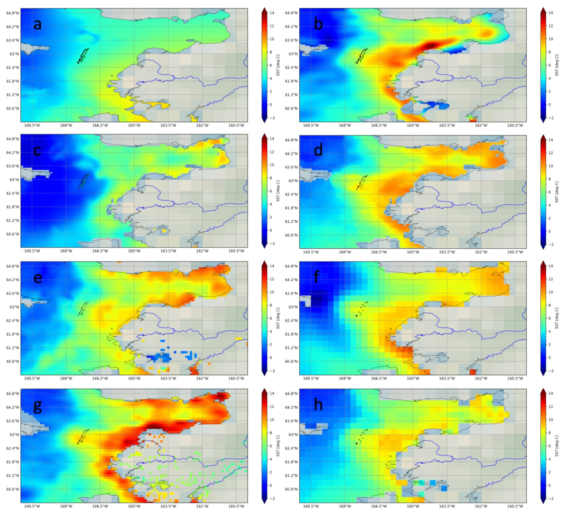
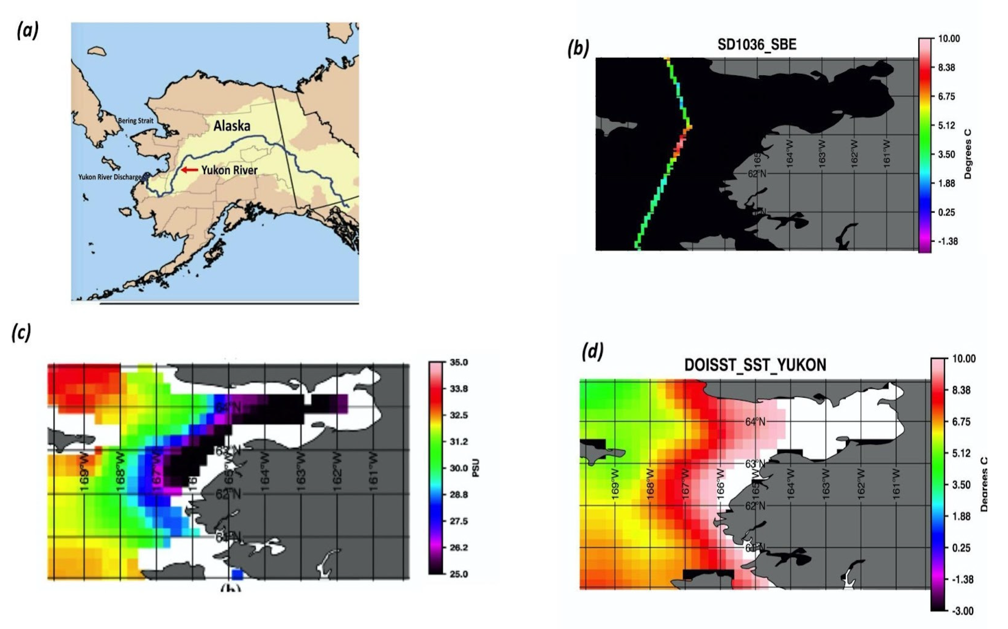
Figure 4 shows images extracted from the different L4 products for the Y–K delta, corresponding to DOY 151. It is notable how the satellite products show substantial differences in the amount of warming near the coast, as well as in the location of these warm features. The coastal variability in SSTs, revealed in Figure 4, is substantial, and it is hard to say which product is more realistic. Relative to the median temperature given by GMPE (Figure 4h), the DOISST, MWIR, OSTIA, and, especially, CMC, retrieve coastal SSTs substantially warmer than the average, whereas MUR, DMI, and K10 are substantially underestimating the warming.
It can be seen that the saildrones navigate across the warm water intrusion that exists between the St. Lawrence Island and the Y–K delta. To get the exact position of thermal fronts from satellite imagery is still very challenging, as the resolution of the L4 grid smears the position of the front. The mesoscale feature, associated with the coastal warmer water, is absent in DMI; it is in a different location in K10 but, as the maps indicate, the saildrones were far enough from the shallow coastal waters of the Y–K delta, missing the highly variable area in the L4 products.

3.1. Statistics

The statistics for the differences between the satellite SST retrievals and SBE temperatures, measured from both saildrone deployments (SD1036 and SD1037), are summarized in Table 2 and Table 3, respectively. The MUR product showed large negative biases for a substantial period of time (DOY 156–212), likely because, in order to produce a foundation SST, this analysis uses satellite nighttime data only, which is a limiting factor during the Arctic summer, as the sun is often above the horizon and nights are often nonexistent. We opted to include another entry in the tables, corresponding to the statistics from the time, where MUR worked well and nighttime data were available. Both time series are used in different comparisons. In those where the trimmed series is used (Taylor diagrams), we will emphasize that the results are for a shorter duration.
The smallest negative biases in Table 2 and Table 3 are observed with the non-foundation products, with the DOISST showing the smallest bias (−0.08 °C) for SD1037, with the second smallest for SD1036 (−0.12 °C) and smallest negative bias with K10 ((−0.11 °C) for SD1036). The DOISST also has the smallest robust unbiased SST estimates (median of the residuals), relative to both saildrone deployments (−0.03 °C and −0.05 °C, respectively). The MWIR OI SSTs also have small residual differences (biased and unbiased (median)), but they are of the opposite sign, suggesting that these MWIR foundation SSTs are slightly warmer than the saildrone measurements (mean biases of 0.05 °C and 0.11 °C, for SD1037 and SD1037, and a median of 0.08 °C and 0.09 °C, respectively). Of the foundation SST products, CMC has the next smallest negative bias (−0.13 °C) for both saildrone deployments. Surprisingly, the GMPE median, established to be a more accurate unbiased estimate of foundation SST than the individual L4 foundation ensemble members (global bias = 0.03 K and SD = 0.4 K relative to Argo floats [8]), had some of the largest mean and median differences, relative to the saildrone observations. This could be due to several factors, which will be discussed later.
It is interesting to note that, despite the fact that all the L4s used in this study are part of the global ensemble (GMPE), the smallest and the largest median error are both observed for SST analyses at the same 0.25°-resolution grid. The large distance between the median DOISST error, with respect to the saildrone and the middle value of the ordered statistics given by GMPE, suggests that the DOISST is more of an outlier in the ensemble. This was quite often the case for DOISST version 2.01, where there was a consistent cold bias for global SSTs and a warm bias for Arctic SSTs; however, existing biases in v.2.0 have been substantially reduced in DOISST v2.1 [18]. The large difference between the DOISST and GMPE might be more in line with the fact that GMPE is an estimator of the foundation whereas the DOISST is a daily mean SST.
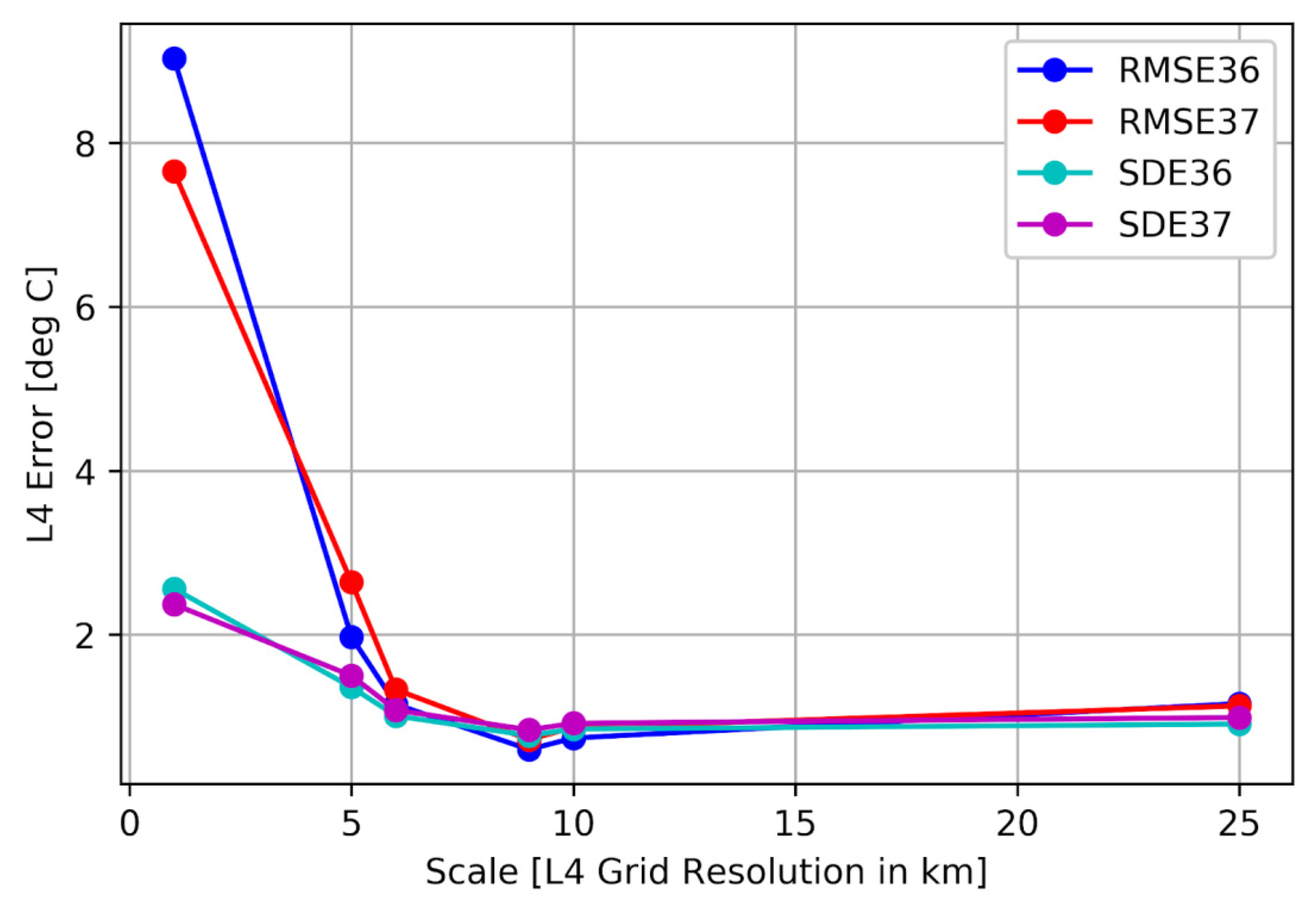
The DOISST minus saildrone SST differences have the smallest variation (SD = 0.74 °C) for SD1036 and the second smallest (SD = 0.88 °C), after the MWIR (SD = 0.84 °C), for SD1037. The SD of the foundation products tends to decrease as the spatial scale (pixel length or/grid spacing) increases (or equivalently, as the sample size/number of co-located pairs decreases with finer product resolution), up to about 9 km, when the SD increases again, as the spatial scale continues to increase (and the sample size continues to decrease), albeit at a slower rate. This issue is illustrated in Figure 5, where the SDs for MUR (1 km), DMI (5 km), and OSTIA (6 km) decrease with scale up to the MWIR 9-km resolution, followed by an increase in SD for CMC, K10 (10 km), and GMPE (25 km). Interestingly, a scale of 9 km is comparable to the local internal Rossby radius of deformation [24]. In the Arctic Ocean, the first Rossby radius increases from ~5–15 km for deep ocean basins, with a typical value of 9–10 km and ~1–7 km for shallow shelf seas [24].
The analyzed pairs incorporate point-to-pixel differences that are influenced by multiple factors. While point to pixel differences can be larger for coarser scales, there is more inherent natural variability at finer spatial scales. It is known that the signal detected from the satellite corresponds to an integration of the surface-emitted radiation over the spatial domain, as determined by the product’s spatial resolution. The signal integration over larger spatial domains/coarser grids smooths out some of the natural variability within the pixel. As the SDE vs. scale trend, shown in Figure 5, suggests, more is not necessarily better for scales < 9 km, as better precision in the estimates (L4 with smaller SDEs) are achieved with smaller sample sizes. This point suggests that caution must be used in interpreting variability at scales less than 10 km, as the noise could be the dominant factor. It is also important to mention that it could also be a natural consequence of increased averaging over the larger spatial scales and thus smoother results. The effects of natural variability and sample variability (sample size) reach a balance at about 9–10 km-spatial resolutions. For scales greater than 9–10 km, the natural smoothing of the gridding process dampens some of the variability and ‘less becomes more’ or at least enough, as the SDEs increase again but at a much slower rate.
The SDE is particularly sensitive to outliers, as large errors are amplified when they are squared in the SDE computation. This tendency is not present in the RD, which is expected, given that this parameter is more effective at handling variability. It is interesting to note that for spatial scales greater than or equal than 10 km, the difference between the SDE and the RD gets smaller (see Table 3). Once again, the convergence of the SDE and the RD at larger scales suggests that the spatial averaging that occurs from increasing the spatial domain/grid resolution of the L4 SSTs is effective at damping the noise (outliers) resulting from natural variability. However, it is important that footprint size alone is not a determining factor in the noise level of satellite products. Other sources of errors exist, including cloud cover, ice contamination (for the Arctic), and possible land contamination in the passive microwave. The L4s with the smallest RD are OSTIA, DOISST, and CMC (with RD of 0.72 °C, 0.73 °C, and 0.80 °C, respectively, for SD1036 and 0.80 °C, 0.87 °C, 0.87 °C, respectively, for SD1037).
The RMSE, while conceptually similar to the SDE, removes some of the randomness in the error estimates and is the standard measure of the accuracy of satellite SST products. Once again, DOISST, MWIR, and CMC are among the products with the smallest RMSE (DOISST: 0.56, MWIR: 0.60, CMC: 0.74 for SD1036, and MWIR: 0.72, DOISST: 0.78, CMC: 0.87 for SD1037). Note that the two products with the better accuracies, DOISST and MWIR, correspond to an SST-at-Depth product and a foundation SST product, respectively. This point suggests that a good precision foundation SST product can perform similarly to a daily mean SST-at-depth product when estimating the Arctic summer SST-at-depth observed from the saildrone.
This result suggests that diurnal variability, although a source of uncertainty, must be considered carefully with respect to other sources of error. Spatial variability, however, seems to have a more substantial effect on L4 foundation accuracy, as the RMSE gets smaller with increasing product spatial resolution, up to a scale of ~9–10 km, after which the RMSE increases, but at a slower rate (see Figure 5). The curves for the two saildrone deployments seem to converge for spatial scales of ~6 km. The separation in mean RMSE amplitudes barely changes as the sample size diminishes from spatial lengths of 10 to 25 km, suggesting that there is a critical scale where the statistical power is associated with the variability of the data and the sample density balances out. The accuracy of the non-foundation products (i.e., DOISST and K10) does seem to follow this trend, as well. This trend is not surprising after the similar behavior observed with the SDs and the known fact that the RMSE is dependent on the scale of the values used. However, Figure 5 shows that, while the SDE dependence on scale appears linear for scales < 10 km, the RMSE dependence, over the same scales, seems to be non-linear convex in shape. Recall from Equations (2) and (3) that the SDE has the mean bias error removed, but the RMSE does not. The nonlinearity of the RMSE curve in Figure 5, hence, is capturing the portion corresponding to the systematic error that is excluded from the SDE and, as is evident in this figure, the RMSE is giving more weight to the largest errors observed at the finest scales. While this newly identified dependence has important implications for gridded satellite products, it remains to be proven that it is universal and is upheld for other products and conditions.
Except for those with the finest resolution, most SST products have an SNR > 2.5. The L4 with the largest SNR is DOISST, with SNR = 3.29 and 3.15 for SD1036 and SD1037, respectively. The statistical correlation between the time series of L4 and saildrone SSTs (final column in Table 2 and Table 3) is very high for all products (>0.90), i.e., the L4 SST products are performing quite well in this region but, once again, the DOISST seems to slightly outperform the others, when it comes to estimating saildrone SSTs.
A possible explanation for the good agreement between the Arctic saildrone-borne SSTs and DOISST retrievals is that the DOISST is highly tied to the available buoy data, which serves as the primary bias correction and calibration of this product. This was made evident, displayed by the DOISST version 2.10, when they stopped feeding a significant percentage of drifting buoys into their system, as the buoy transmissions changed from alpha-numerical to binary form [18]. In-situ measurements, while ingested in some of the other L4 analyses, potentially do not play as critical a role, as they rely more on the multisensor blending aspect of the satellite retrievals.
The DOISST implicitly adjusts all the input data streams that enter into their OI system to coincide with the buoy measurements at approximately 20 cm-depth. It is important to point out, however, that the saildrone is not incorporated in the DOISST correction and, thus, these are truly independent measurements. Both the saildrone and the buoys use sea bird-type thermistors to measure the SST-at-depth.

3.2. Taylor Diagrams

It is clear from the above analysis that the statistics in Table 2 and 
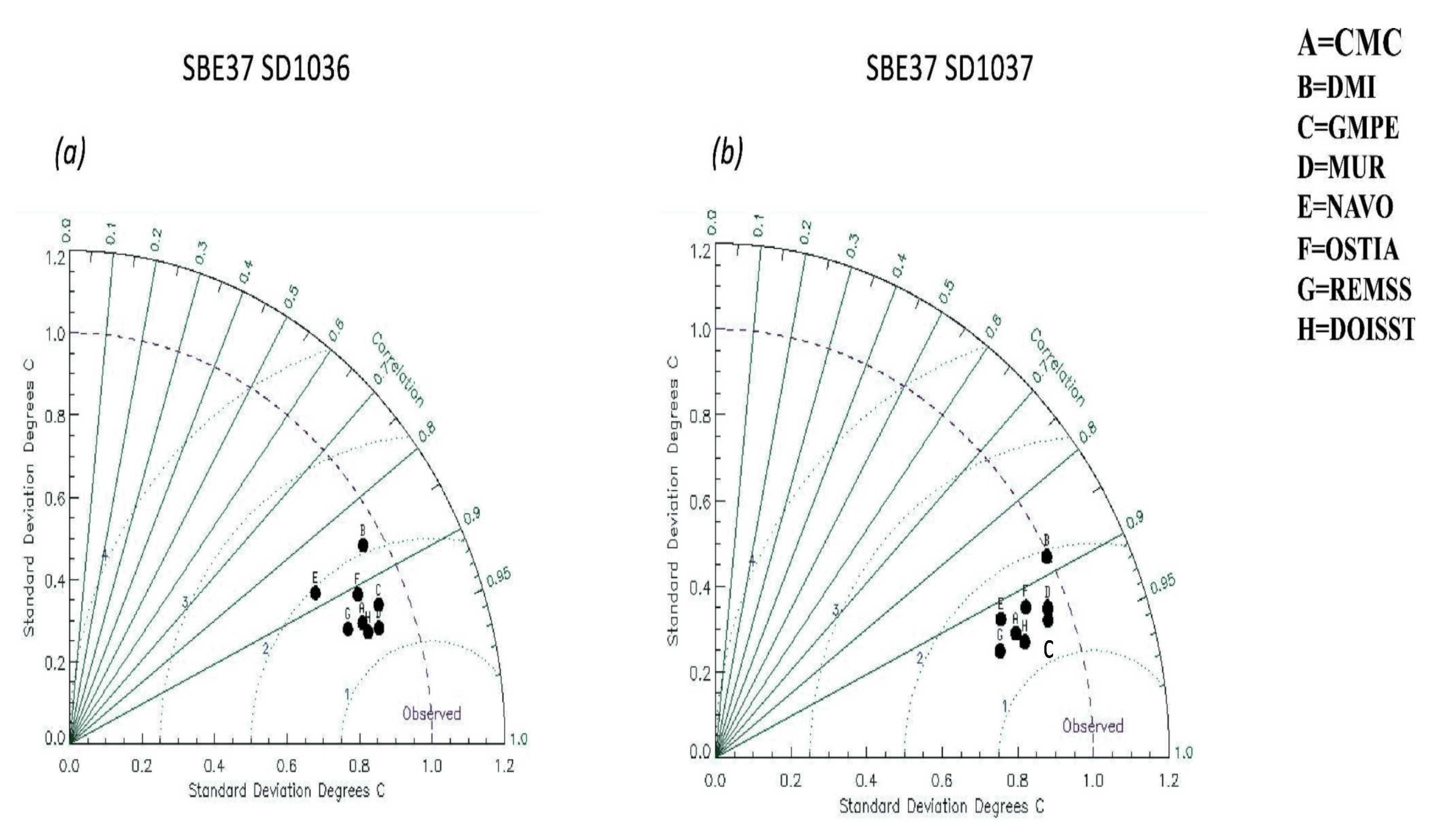
Table 3 are simultaneously constrained by both the disparity in sample sizes of the L4 vs. saildrone SST matchups and the variability of the data itself. In order to facilitate comparisons of L4 products with different scales, normalized statistics were computed using the background variability or SD of the reference SST (i.e., the SDSAIL) as the normalization variable. By using the SDSAIL (via Equation (5)) as the standardizing criterion, we are removing the impact of the variability in the saildrone observations from the interdependence of the statistical measures. We then looked at the simultaneous behavior of the normalized SDs, from both the L4 and observations (i.e., NSDSAT = SDSAT/SDSAIL; NSDSAIL = SDSAIL/SDSAIL = 1), the normalized RMSE (i.e., NRMSE = RMSE/SDSAIL), and their serial correlation, through a normalized Taylor diagram. These are shown in Figure 6a,b for SD1036 and SD1037, respectively. A detailed explanation of how to interpret these diagrams for comparing the performance of different L4 SST products can be found at [10].
The normalized standard deviation (NSD) of the observations is represented in the diagram by the point where the x-axis equals 1, labeled “observed.”. The NSDSAT for the different L4s is given in the y-axis. The dashed circle of unit radius also gives an indication of where the products being compared stand, in relation to the ‘denoised’ observations. The NRMSE is represented by the concentric circles, centered at the observation point (x = 1). The correlations are given by the radial lines departing from the origin (x = 0). The objective is to quickly determine which products, represented by the dots labeled A through H, are closer to the point/dash circle representing the observations. The closer an L4 is to the observations, the smaller the SD and the RMSE and the higher the correlation.
As it can be seen from these diagrams that all the L4 products, represented by the dots, labeled A: CMC, B: DMI, C: GMPE, D: trimmed MUR, E: K10, F: OSTIA, and G: MWIR, H: DOISST, have similar performances and are in overall good agreement with the saildrone, given that all the dots cluster together close to the observations and there is no spread in the radial direction. The products less affected by the variability/noise in the observations, i.e., closer to the dashed circle of the denoised observations, are GMPE, trimmed MUR, and DMI (C, D, and B). Products more affected by systematic errors (i.e., farther from the unit circle) are K10 and MWIR (E and G). The products with better accuracy (closer to the smallest NRMSE circle), and the highest correlations (smallest azimuthal angle between the L4 dot and the x-axis), are the DOISST and the trimmed MUR (H and D) for SD1036 and DOISST and GMPE (H and C) for SD1037. The products with degraded accuracy are K10 for SD1036 and DMI for SD1036 and SD1037. The fact that DMI is closest to the dashed unit circle but has the largest azimuthal spread (correlation less than 0.9) suggests the product is getting the right SST amplitudes but has issues with the phasing of the SST patterns.
The products that have the best overall performance, based on the smallest absolute distance to the observations, are GMPE, DOISST, and the trimmed MUR (C, D, and H). As the Taylor diagram illustrates, the DOISST remains a top performer, regardless of the normalization of the statistics, but two of the L4 products that were more impacted by noise in the saildrone observations before (e.g., GMPE and the untrimmed MUR in Table 2 and Table 3), perform substantially better relative to the saildrone observations. The GMPE result confirms previous analyses reported in the literature [8], indicating that it was the noise in the saildrone observations driving the spread in the statistics. When nighttime data are available, the MUR L4 could be a leading performer. The MUR product is currently being analyzed to include daytime observations for the estimation of the foundation SST, which will take effect in the next version of MUR (M. Chin, personal communication, 2021).
Among the products with slightly diminished skill after the normalization are DMI, K10, and MWIR (C, E, and G). After taking the saildrone variability out, the K10 and the MWIR, which had a leading edge according to the statistics of Table 2 and Table 3, are now further to the left from the actual SD given by the unit circle, NSDSAIL = 1. In other words, the NSD is decreasing with noise in these two products, which suggests that they are under-predicting the observed saildrone variability (i.e., they are a bit smooth). The K10 in particular was singled out before as being the same type of SST as the SBE37 SST, which was thought to be advantageous for comparisons with the saildrone. It is known that the lack of an ice mask slightly undermines the K10 predictions, when in close proximity to the ice edge. The K10 product is currently being modified to include an ice mask in a new future version [J.F. Cayula, personal communication, 2021]. In previous comparisons involving the MWIR SST, the product appeared to have too much small-scale noise [10]. In its current version (version 5), however, Figure 6 suggests that this analysis is under-predicting the actual saildrone variability. The NRMSE and correlation, however, are not perturbed enough by the noise, since the MWIR dot is part of the general cluster.

3.3. Wavelength Spectra

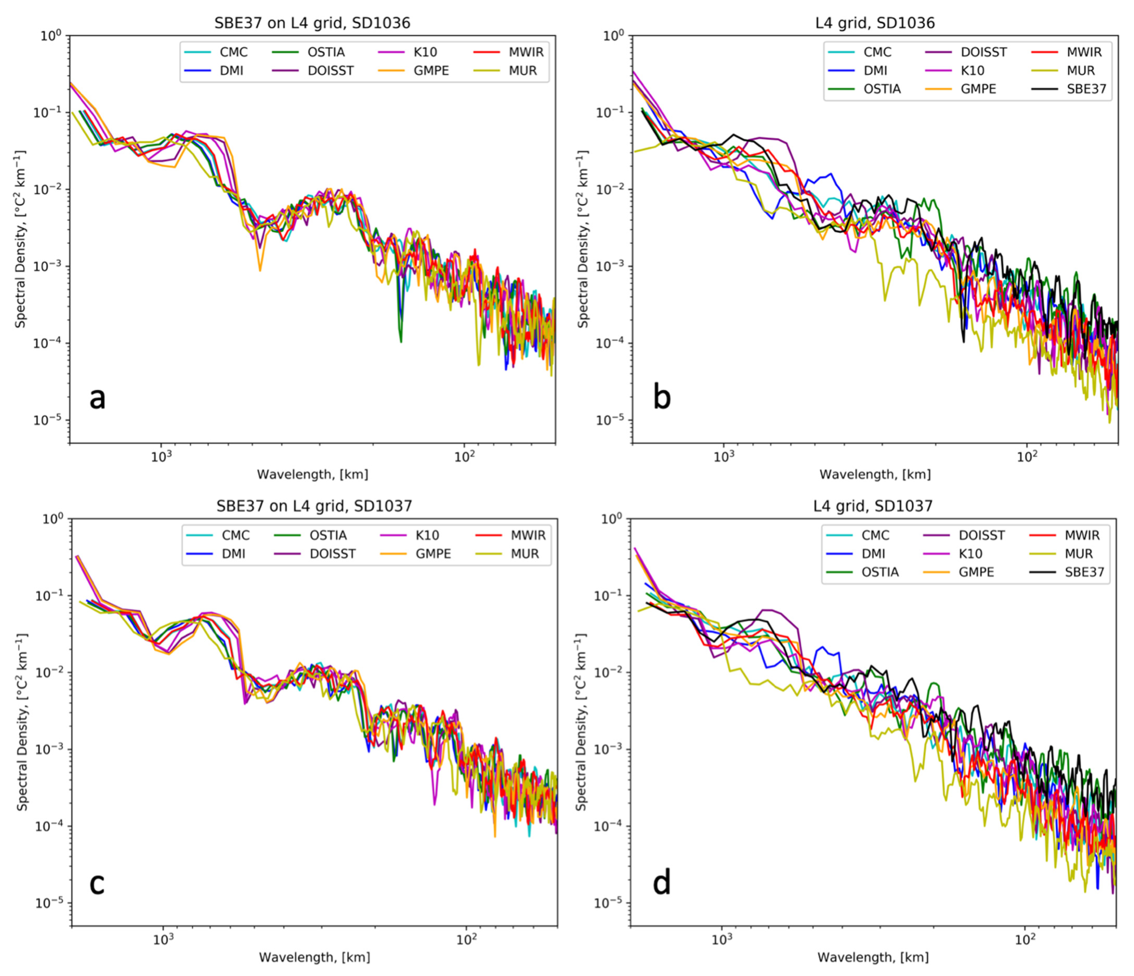
In order to further explore the dependence of spatial variability on spatial scales, spectral analysis was performed on each of the L4 products and the saildrone SSTs. Wavelength spectra were calculated based on the co-located data, which means that there is a saildrone power spectrum for each of the satellite products (only the grid resolution varies). The entire time series of the products were used, DOY 135–283. Thus, the saildrone power spectra are reflective of the resolution of the GHRSST L4 product. For the MUR product, the whole length of the time series was considered in the spectral analysis. The resulting plots are shown in Figure 7 for both SD1036 and SD1037 with the saildrone Fourier autospectra on the left panel, and the L4 SST on the right.
The saildrone SST spectra shown on the left were computed from the SBE37 collocations with the different SST analyses. That is, the only thing that is changing is the spatial resolution of the subsampling of the saildrone SBE37 SSTs. The spectra are plotted only for wavelengths greater than 50 km to reflect the Nyquist wavelength associated with the DOISST and GMPE products, which have the coarser spatial resolution of the L4s used in this spectral analysis. The saildrone-derived power spectral density, shown in black with the L4 autospectra of Figure 7b,d, is based on the co-locations with OSTIA. This particular subsampling of the saildrone spectrum was chosen because, as it will be explained in more detail in the analysis of spectral slope below, only OSTIA appears to have the same scaling relation observed with the saildrone-derived SSTs.
The most visible feature of the spectra shown in Figure 7 is the power law behavior (i.e., the log-log linearity as the log of the spectral power decreases with the log of the decreasing wavelength) exhibited by all the autospectra over the whole range of measurement scales (between 2000 km and 50 km). Additionally, the rate of decrease (given by the spectral slope or, in this case, the scaling exponent) appears quite similar for the individual autospectra, suggesting scale invariance. The saildrone spectra in Figure 7a,c show peaks at approximately 1000 and 500 km. One possible explanation is these arise when a saildrone changes trajectory. However, this would require further research to confirm and is only speculative.
Overall, for wavelengths < 100 km, the spectral densities of the L4s are lower than those derived from the SBE37 SSTs, reflective of the higher spatial sampling of the in-situ instruments deployed on the saildrone. It is important to note that spectra < 100 km were found to be statistically different from zero, based on the derivation of error bars. Note that for this mesoscale regime, only OSTIA matches saildrone, with the others showing a slight drop in power density.
For scales > 200 km, the saildrone spectra flattened slightly, indicating white noise. The saildrone deployment takes place over several months and, thus, over the larger spatial scales the assumption of a synoptic scale is not valid. The L4 power density spectra in general show increasing power for scales > 200 km, indicating that the satellite products are resolving the large-scale fluctuations better than saildrone. However, this must be interpreted with caution as the spectra were derived assuming a synoptic-scale over the entire saildrone deployment. Overall, results are encouraging indicating that the GHRSST L4 SST products are replicating the power spectral density associated with the saildrone SBE37 SSTs.

3.4. Spectral Slopes

The power spectral density slopes (or scaling exponent of the power-law suggested by the log-log linearity of the Fourier power spectra) were determined for each of the individual autospectrum shown in Figure 7. The slope was determined by a simple linear regression fit to the log(power spectral density) versus the log(wavelengths). Slopes for the SBE37 SST autospectra from both the SD1036 and the SD1037, sampled on the different L4 grids, are shown on the left column of Table 4. Slopes for the GHRSST L4 autospectra are shown on the right.
Spectral slopes are tabulated and sorted by the size of the L4 grid. It can be seen from Table 4 that the saildrone slope becomes increasingly negative (i.e., the drop in power becomes slightly steeper) with increasing spatial resolution of the L4 product in which it is subsampled. In fact, the increase in negative slope appears to be roughly 0.01 °C 2 km−1 per kilometer increase in satellite grid length used to subsample the saildrone-derived SSTs. This appears to be the case for both saildrone deployments, but with SD1037 showing more transparently the dependence just described. Taking DMI as the reference, L4 slope = −1.76 + 0.01 × (5 km − grid size [in km]).
Overall, the log-log negative slopes associated with the co-located saildrone data are less negative (shallower) than those associated with the GHRSST L4 SST products, with an average slope of −1.84 (Table 4, left column). This is in very good agreement with the SST scaling exponent of −1.80 reported by [25] using a 2-D power spectrum and a direct scaling moment function on MODIS Aqua SST images to characterize fluctuations of velocity and SST [25]. The log-log slopes of the different L4 wavelength spectra (Table 4, right column), on the other hand, vary approximately between −2.12 for SD1036 and −2.23 for SD1037. These values are also in good agreement with previous slopes of Fourier power spectrum of satellite-derived SSTs reported in the literature. [25,26] reported a slope of −2.44. Note that the DOISST had a slope of −2.39 for the SD1037). This difference between the saildrone and L4 spectra is seen across all the grids in which the saildrone spectrum is subsampled, with the exception of OSTIA. The OSTIA spectral slope is the only one that coincides with that of the saildrone when subsampled on its grid (see Table 4. OSTIA slope ~1.8 vs. saildrone on OSTIA grid ~1.78). This result suggests that only the OSTIA SST product is reproducing the small-scale spatial variability observed from in situ instruments more accurately than the other satellite products.
The saildrone exponent of −1.8 is slightly steeper but closer to the −5/3 spectral slope of the Kolmogorov power law for temperature fluctuations in the inertial range, displaying characteristics of passive scalar (temperature is advected with the flow) fully developed turbulence. The SST spectral slopes of −2 are consistent with the presence of submesoscale processes at the ocean surface in the Arctic Ocean and other oceanic regions [27,28,29].

4. The Arctic River Discharge in the Yukon–Kuskokwim (Y–K) Delta: A Case Study

Previous work [13] compared SSS from NASA’s Soil Moisture Active Passive (SMAP) satellite and saildrone-derived SSS and concluded that both the saildrone and the SMAP were observing freshening, associated with the Y–K delta (Figure 8c). Figure 8b shows that similarly, saildrone-derived SSTs show an increase in temperature near the delta. We focus now on further evaluating whether the observed warming in the Y–K delta is consistent with the freshening due to the rivers’ discharge.
We focus on three data sets: DOISST, OSTIA, and the MWIR SSTs. OSTIA appears to have more spectral power than the other data sets for scales < 100 km and is able to better resolve the fine-scale fluctuations according to the spectra plots in Figure 7b,d. This is further supported by visual inspection of Figure 4b, where the warm SST coastal features in the OSTIA image are directly located at the mouths of both the Yukon and Kuskokwim rivers. The warm water from the Kuskokwim River is also evident in DOISST (Figure 4f), but the signature from the Yukon River is less defined. Further, the spectral slope of OSTIA (1.78 and 1.82 for SD1036 and SD1037 in Table 4) is closer to the theoretical slope of −2, where submesoscale processes are suspected to be present at the surface. Being able to resolve the submesoscales is of critical importance for the study of estuarine processes e.g., [27].
Although the statistics for the MWIR were a bit mixed, the time series of SST around the Y–K delta shows very good agreement with the saildrone. Figure 3a,b shows that, at the peak of the Y–K delta warming, during day 151, only the MWIR and the CMC captured the right amplitude and location of the warming observed by the saildrones. This resulted in ~zero biases for these two products during the period of 150–153, as seen in Figure 3b. Further, the MWIR thermal spatial variability (Figure 4d) is similar to OSTIA’s (Figure 4b).
The DOISST composite over the Y–K delta region (60° N to 65° N and 167° W to 170° W) and entire saildrone campaign (150 days) is shown in Figure 8d. Comparing Figure 8c,d, one can see that there is a freshening (local minima) in SSS coinciding with the warmer (local maxima) SSTs, associated with river discharge from the Yukon and the Kuskokwim rivers.
Next, an SMAP-derived SSS climatology is compared to the Y–K delta, against SST climatology’s, for the same time period from DOISST and OSTIA (Figure 9).
Seasonal freshening in the ocean west of the Y–K delta is generally associated with warmer temperature, as opposed to normal coastal upwelling conditions, where cooler temperatures are associated with saltier waters. Additionally, if one examines the cross-correlation between the two time series (not shown), the maxima correlation occurs at 0-lag, indicative of both the freshening and warming occurring simultaneously. These facts provide additional support to the hypothesis that the thermal signal, seen by the satellite and the saildrones SSTs off the Y–K delta, is, indeed, associated with river discharge.

5. Summary and Discussion

The purpose of the research is not to determine the best GHRSST SST analysis for Arctic applications, but to show results in such a way that can lead to further improvements in satellite-derived SST products at high latitudes, where they play a critical role in monitoring changes in this part of the world’s oceans.
The results of this L4 inter-comparison, with respect to saildrones, are encouraging because they show substantial improvements in the high-latitude SST analyses, at least in open waters, compared to their performance six years ago (see Figure 5 and Figure 6 from [10]). There are still substantial differences among products in coastal areas and dynamic regions-like river outlets, as the SST maps of the Y–K delta, shown in Figure 4a–h, suggest. Limitations of the study include that the wavenumber Fourier spectra assume a synoptic scale over the duration of the saildrone deployments. This is obviously not the case. Additionally, the comparison is restricted to one year, so conclusions about data sets could be specific to 2019. Thus, caution should be taken in generalizing results to other years.
The extreme warming differences observed in coastal regions brings into question the meaning of a foundation SST for shallow coastal regions, in particular for the Arctic Seas, where there is an extended period of warming during the Arctic summer. If warming penetrates all the way to the bottom of the ocean, what is the meaning of the foundation SST under those conditions?
Of all the L4 foundation SSTs considered here, it is hard to say, judging by the wide range of warm SST amplitudes in shallow coastal waters, which one is giving a more realistic foundation estimate. Relative to the median ensemble GMPE, then there are L4 products that are underestimating coastal warming (i.e., MUR, DMI, and K10) and others that are substantially overestimating this warming (i.e., DOISST, MWIR, OSTIA, and CMC). Of the three products that are underestimating coastal warming, two, MUR and DMI, estimate foundation SSTs based solely on nighttime observations. This reduces the data availability of the single sensor SSTs that are being ingested into the analysis systems; thus, alternative foundation estimate techniques should be considered; however, at a minimum, daytime data must be included for high latitude SST retrievals. Of the products that are producing warmer foundation SSTs in coastal regions, the MWIR appears to be the most consistent with GMPE. As it happens, this is the only L4 product that uses a diurnal warming model in its estimate of the foundation. Clearly, SST analyses would benefit from exploring the inclusion of a diurnal warming model, at least for coastal regions.
The global statistics are shown in Table 2 and Table 3, as well as the Taylor diagrams (Figure 6), which pointed to the DOISST product as the candidate with a leading edge in these comparisons. This is a product that relies entirely on IR and in situ data and, as a result, should be at a disadvantage in the Arctic, due to increased cloudiness in the region. The main difference between the DOISST and other L4s considered here is its stronger reliance on in situ data from buoys and Argo floats. Thus, it appears that products that rely more heavily on in situ observations do better in the Arctic oceans.
The accuracy of SST analyses depends on using as much high-resolution data as possible. The high-resolution data are provided by the IR sensors, but IR SST retrievals are limited to clear skies and good weather conditions. When the IR coverage is poor, the analyses are prone to generate high-frequency noise [10,30,31,32]. The high-resolution data are particularly important near the ice edge and coastal regions, since the coarser MW SSTs are not retrieved within 75 km of ice or land. These same regions happen to be areas of enhanced natural variability [27]. The disparity in MW vs. IR resolution makes the analyses extremely susceptible to the availability of fine-resolution IR data, which is not always attainable, due to increased cloudiness in the Arctic region. Improvements in coastal areas, however, can be achieved by using adaptive correlation scales, with shorter length scales in highly variable regions [33], as seems to be shown here with OSTIA.
It is clear that there is substantial spatial SST variability at high latitudes. This implies that not only the availability but also the abundance of high-resolution data is particularly important for high-resolution SST analyses. A key finding from Figure 5 is the suggested dependence between spatial variability and sample density variability or, equivalently, between product accuracy and L4 grid resolution. This dependence was observed for the SDE and the RMSE, with the former appearing linear and the latter nonlinear. The gap between robust statistics and standard statistics (Table 2 and Table 3) also narrowed for scales ≥10 km. This would also be consistent with the Rossby number in the Arctic, which is < ~10 km. The dependence plot suggests that, for spatial resolutions < ~9–10 km, the noise in the analyses tends to dominate over the physical signal (due to small-scale variability and limited high-resolution data availability). This finding implies that to fully resolve the spatial variability associated with the Arctic, increased availability of high-resolution observations with reduced noise is required in the Arctic. In the absence of these data, coarser-resolution SST products may actually provide a more accurate representation at their corresponding scale. This highlights the challenges of producing SST analyses of ultra-high spatial resolution in the Arctic regions with current satellite technology. The L4 analyses that performed best, statistically, with respect to the saildrone, were all on the side of the dependence relationship where the natural smoothing that results from binning the SSTs over coarser resolution grids dumped the noise from spatial variability within the grid cells (e.g., grid resolutions greater or equal than ~6 km).
There is a paradox in Figure 5, in that SST analyses tended to reproduce more small-scale spurious features (noise) the finer the spatial resolution of the product. Similarly, the coarser the spatial resolution of the SST product, the more accurate the product appears to be relative to the saildrone data aggregated over the pixel, presumably because of the more effective smoothing of the inherent natural variability at the larger grid cells. It is important to bear in mind that these are analyzed products that blend multi-resolution products; as such, we can only speculate as to the sources of the observed variability. For a better understanding of the dependence between satellite footprint and SST spatial variability at the subpixel level, see [33].
Of course, there is a difference between spatial resolution and the feature resolution of the satellite product. The L4 product that was most successful, in terms of resolving the fine-scale features associated with the dynamics of the coastal region appears to be OSTIA. This was evidenced in the spectral plots and can be confirmed by looking at the satellite images for DOY 151. This product is the only one that showed evidence of warm patches associated with the river discharge in the Y–K delta and right locations. Other products show warming at one of the river’s mouths, but not the other, or show the entire coast as warm or not warm at all. In the past, this product was known for its smoothness (despite its ~6-km spatial resolution, the product had a feature resolution of 10 km [17]). Starting in 2016, however, the OSTIA system started ingesting the ultra-high resolution VIIRS and made adjustments that improved its feature resolution. This change resulted in an improvement of OSTIA to represent small-scale features, without introducing noise [34], and our analyses certainly gives external validity to this claim for the Arctic coastal regions.
Caution should be exercised when choosing a satellite product to use in a particular application, based on the interpretation of the statistics alone. The outcomes of this study were somewhat different, whether standard or robust statistics were analyzed or the data was standardized by the natural variability of the saildrone. Even spectral analysis gave a different outcome for the L4 analysis that better reproduced the fine-scale variability being resolved by the saildrone. Even though all these products are performing quite well in the open oceans (high correlations and SNR), substantial differences still persist in highly dynamic areas, such in coastal regions. Using global statistics alone, one can get the correct answer for the wrong reasons, or vice versa, if not looking at these comparisons in a more comprehensive way. In the end, nothing beats visual inspection to decide what works best for one’s particular application. Our results also show that regional comparisons are necessary for establishing which product is most suitable for a specific application. Future work needs to extend comparisons to other years, as well as more rigorous analysis of how both the optimal interpolation technique used, as well as input data sets into the L4 analysis, lead to differences in the overall quality in the Arctic. Another area of work would be to determine how possible issues of cloud masking are affecting the quality of SST retrievals in the Arctic. This would be especially critical to resolving the impact of changes in river discharge in coastal regions, such as the Y–K delta, where the higher resolution IR data is critical for the feature resolution needed.

Author Contributions

Conceptualization, J.V.-C., S.L.C.; methodology, J.V.-C., S.L.C.; software, C.G., S.L.C.; writing—original draft preparation, J.V.-C., S.L.C.; writing, S.L.C.—review and editing, all; visualization, all writing and editing, M.S.; writing and editing, W.T., J.G.-V., S.L.C. All authors have read and agreed to the published version of the manuscript.

Funding

This research was supported by NASA, through the Multi-Sensor Improved Sea Surface Temperature (MISST) project. JGV was supported by CICESE and CONACYT, México. Sandra Castro, Michael Steele, and Chelle Gentemann were funded by the MISST3 Project, NASA grant 80NSSC20K0768. M. Steele was also funded by NASA grants NNX16AK43G and 80NSSC20K0134, NSF grant PLR 1603266 and ONR grant N00014-17-1-2545.

Institutional Review Board Statement

The manuscript went through the internal review process at the Jet Propulsion Laboratory/Institute of Technology.

Data Availability Statement

SST products, along with the two saildrone deployments, were downloaded from PO.DAAC. The products from the Remote Sensing System products may be downloaded from: http://podaac.jpl.nasa.gov (from:https://podaac.jpl.nasa.gov/dataset/SMAP_JPL_L3_SSS_CAP_8DAY-RUNNINGMEAN_V43?ids=&values=, accessed on 9 December 2021). Saildrone data can also be downloaded through the PO.DAAC, at: https://podaac.jpl.nasa.gov/dataset/SAILDRONE_ARCTIC?ids=&values= (accessed on 9 December 2021).

Acknowledgments

We would like to thank Rachel Spratt, a NASA postdoctoral at JPL, for editing the manuscript.

Conflicts of Interest

The authors declare no conflict of interest.

References

  1. Steele, M.; Dickinson, S. The phenology of Arctic Ocean surface warming. J. Geophys. Res. Ocean. 2016, 121, 6847–6861. [Google Scholar] [CrossRef] [PubMed]
  2. Screen, J.A.; Simmonds, I. Increasing fall-winter energy loss from the Arctic Ocean and its role in Arctic temperature amplification. Geophys. Res. Lett. 2010, 37, L16707. [Google Scholar] [CrossRef] [Green Version]
  3. Jackson, J.M.; Carmack, E.C.; McLaughlin, F.A.; Allen, S.E.; Ingram, R.G. Identification, characterization, and change of the near-surface temperature maximum in the Canada Basin, 1993–2008. J. Geophys. Res. 2010, 115, C05021. [Google Scholar] [CrossRef]
  4. Jackson, J.M.; Williams, W.J.; Carmack, E.C. Winter sea-ice melt in the Canada Basin, Arctic Ocean. Geophys. Res. Lett. 2012, 39, L03603. [Google Scholar] [CrossRef]
  5. Steele, M.; Ermold, W.; Zhang, J. Modeling the formation and fate of the near-surface temperature maximum in the Canadian Basin of the Arctic Ocean. J. Geophys. Res. 2011, 116, C11015. [Google Scholar] [CrossRef] [Green Version]
  6. Timmermans, M.; Jayne, S.R. The Arctic Ocean Spices Up. J. Phys. Oceanogr. 2016, 46, 1277–1284. [Google Scholar] [CrossRef]
  7. Dean, K.G.; Mcroy, C.P.; Ahlnas, K.; Springer, A. The Plume of the Yukon River in Relation to the Oceanography of the Bering Sea. Rem. Sens. Environ. 1989, 28, 75–89. [Google Scholar] [CrossRef]
  8. Martin, M.; Dash, P.; Ignatov, A.; Vanzon, V.; Beggs, H.; Brasnett, B.; Cayula, J.F.; Cummings, J.; Donlon, C.; Gentemann, C.; et al. Group for High Resolution Sea Surface Temperature (GHRSST) analysis fields inter-comparisons. Part 1: A GHRSST multi-product ensemble (GMPE). Deep Sea Res. Part II 2012, 77–80, 21–30. [Google Scholar] [CrossRef]
  9. Dash, P.; Ignatov, A.; Martin, M.; Donlon, C.; Brasnett, B.; Reynolds, R.W.; Banzon, V.; Beggs, H.; Cayula, J.F.; Chao, Y.; et al. Group for High Resolution Sea Surface Temperature (GHRSST) analysis fields inter-comparisons—Part 2: Near real time web-based level 4 SST Quality Monitor (L4-SQUAM). Deep Sea Res. Part II Top. Stud. Oceanogr. 2012, 77–80, 31–43. [Google Scholar] [CrossRef] [Green Version]
  10. Castro, S.L.; Wick, G.; Steele, M. Validation of sea surface temperature analyses in the Beaufort Sea using UpTempO buoys. Remote Sens. Environ. 2016, 187, 458–475. [Google Scholar] [CrossRef]
  11. Castro, S.L.; Wick, G.; Buck, J.J.H. Comparison of diurnal warming estimates from unpumped Argo data and SEVIRI satellite observations. Remote Sens. Environ. 2014, 140, 789–799. [Google Scholar] [CrossRef] [Green Version]
  12. Eastwood, S.; Le Borgne, P.; Péré, S.; Poulter, D. Diurnal variability in sea surface temperature in the Arctic. Remote Sens. Environ. 2011, 115, 2594–2602. [Google Scholar] [CrossRef]
  13. Vazquez-Cuervo, J.; Gentemann, C.; Tang, W.; Carroll, D.; Zhang, H.; Menemenlis, D.; Gomez-Valdes, J.; Bouali, M.; Steele, M. Using saildrones to Validate Arctic Sea-Surface Salinity from the SMAP Satellite and from Ocean Models. Remote Sens. 2021, 13, 831. [Google Scholar] [CrossRef]
  14. Brasnett, B. The impact of satellite retrievals in a global sea-surface-temperature analysis. Q. J. R. Meteorol. Soc. 2008, 134, 1745–1760. [Google Scholar] [CrossRef]
  15. Hoyer, J.L.; Le Borgne, P.; Eastwood, S. A bias correction method for Arctic satellite sea surface temperature observations. Remote Sens. Environ. 2013, 146, 201–213. [Google Scholar] [CrossRef]
  16. Fiedler, E.K.; Mao, C.; Good, S.A.; Waters, J.; Martin, M.J. Improvements to feature resolution in the OSTIA sea surface temperature analysis using the NEMOVAR assimilation scheme. Q. J. R. Meteorol. Soc. 2019, 145, 3609–3625. [Google Scholar] [CrossRef]
  17. Donlon, C.J.; Martin, M.; Stark, J.; Roberts-Jones, J.; Fiedler, E.; Wimmer, W. The Operational Sea Surface Temperature and Sea Ice Analysis (OSTIA) system. Remote Sens. Environ. 2012, 116, 140–158. [Google Scholar] [CrossRef]
  18. Huang, B.Y.; Liu, C.Y.; Banzon, V.; Freeman, E.; Zhang, H.M. Improvements of the Daily Optimum Interpolation Sea Surface Temperature (DOISST) Version 2.1. J. Clim. 2021, 34, 2923–2939. [Google Scholar] [CrossRef]
  19. Xu, F.; Ignatov, A. In situ SST Quality Monitor (iQuam). J. Atmos. Ocean. Technol. 2014, 3, 164–180. [Google Scholar] [CrossRef]
  20. Chin, T.M.; Vazquez-Cuervo, J.; Armstrong, E.M. A multi-scale high-resolution analysis of global sea surface temperature. Remote Sens. Environ. 2017, 200, 154–169. [Google Scholar] [CrossRef]
  21. Martin, M.; McLaren, A. Product User Manual for Global Ocean GMPE Sea Surface Temperature Multi Product Ensemble SST_GLO_SST_L4_NRT_OBSERVATIONS_010; Version 3.4, CMEMS Version Scope; Met Office: Exeter, UK, 2015. [Google Scholar]
  22. Gentemann, C.L.; Scott, J.P.; Mazzini, P.L.F.; Pianca, C.; Akella, S.; Minnett, P.J.; Cornillon, P.; Fox-Kemper, B.; Cetinic, I.; Chin, T.M.; et al. Saildrone: Adaptively sampling the marine environment. Bull. Am. Meteorol. Soc. 2020, 101, 744–762. [Google Scholar] [CrossRef] [Green Version]
  23. Rousseeuw, P.J.; Croux, C. Alternatives to the Median Absolute Deviation. J. Am. Stat. Assoc. 1993, 88, 1273–1283. [Google Scholar] [CrossRef]
  24. Nurser, A.J.G.; Bacon, S. The Rossby radius in the Arctic Ocean. Ocean. Sci. 2014, 10, 967–975. [Google Scholar] [CrossRef] [Green Version]
  25. Renosh, P.; Schmitt, F.G.; Loisel, H. Scaling Analysis of Ocean Surface Turbulent Heterogeneities from Satellite Remote Sensing: Use of 2D Structure Functions. PLoS ONE 2015, 10, e0126975. [Google Scholar] [CrossRef] [PubMed]
  26. Abraham, E.R.; Bowen, M.M. Chaotic stirring by a mesoscale surface-ocean flow. Chaos 2002, 12, 373. [Google Scholar] [CrossRef] [PubMed] [Green Version]
  27. Castro, S.L.; Emery, W.J.; Wick, G.A.; Tandy, W. Submesoscale Sea Surface Temperature Variability from UAV and Satellite Measurements. Remote Sens. 2017, 9, 1089. [Google Scholar] [CrossRef] [Green Version]
  28. Timmermans, M.; Cole, S.; Tool, J. Horizontal density structure and restratification of the Arctic Ocean surface layer. J. Phys. Oceanogr. 2012, 42, 659–668. [Google Scholar] [CrossRef] [Green Version]
  29. Huang, Y.; Wang, L. Cascade and intermittency of the sea surface temperature in the oceanic system. Phys. Scr. 2019, 94, 014009. [Google Scholar] [CrossRef] [Green Version]
  30. Chelton, D.B.; Wentz, F.J. Global Microwave Satellite Observations of Sea Surface Temperature for Numerical Weather prediction and Climate Research. Bull. Am. Meteorol. Soc. 2005, 86, 1097–1115. [Google Scholar] [CrossRef] [Green Version]
  31. Reynolds, R.W.; Smith, T.M.; Liu, C.; Chelton, D.B.; Casey, K.S.; Schlax, M.G. Daily high-resolution blended analyses for sea surface temperature. J. Clim. 2007, 20, 5473–5496. [Google Scholar] [CrossRef]
  32. Reynolds, R.W.; Chelton, D.B.; Roberts-Jones, J.; Martin, M.J.; Menemenlis, D.; Merchant, C.J. Objective determination of feature resolution in two sea surface temperature analyses. J. Clim. 2013, 26, 2514–2533. [Google Scholar] [CrossRef] [Green Version]
  33. Castro, S.L.; Monzon, L.A.; Wick, G.A.; Lewis, R.D.; Belkin, G. Subpixel variability and quality assessment of satellite sea surface temperature data using a novel High Resolution Multistage Spectral Interpolation (HRMSI) technique. Remote Sens. Environ. 2018, 217, 292–308. [Google Scholar] [CrossRef]
  34. Roberts-Johns, J.; Bovis, K.; Martin, M.J.; McLaren, A. Estimating background error covariance parameters and assessing their impact in the OSTIA system. Remote Sens. Environ. 2016, 176, 117–138. [Google Scholar] [CrossRef]
Figure 1. SST, derived from SBE37, along with the saildrone track for SD1036 (a) and SD1037 (b). The location of Y–K delta and rivers are shown in (c).
Remotesensing 14 00692 g001
Figure 2. Time series of GHRSST L4 SST products, co-located with the SBE37 SSTs, onboard saildrones (a) SD1036 and (b) SD1037.
Remotesensing 14 00692 g002
Figure 3. (ad) SST amplitudes (top (a,b)) and L4 biases, relative to the SBE37 SSTs (bottom, (c,d)), while the saildrones were traversing the Y–K delta on 31 May 2019 (DOY 151). The left column is for SD1036, and the right is for SD1037.
Remotesensing 14 00692 g003
Figure 4. (ah) L4 SST images around the Y–K delta for DOY 151 (31 May 2019) for: (a) MUR, (b) OSTIA, (c) DMI, (d) MWIR, (e) K10, (f) DOISST, (g) CMC, and (h) GMPE. The black dotted line shows the transect of SD1036 for the same day. The green dotted line shows the corresponding track for SD1037. Each saildrone matching position is in the corresponding resolution of the L4 product. For identification of the Yukon river in the image, see Figure 1c.
Remotesensing 14 00692 g004
Figure 5. Dependence of L4 variability on the scale. Comparison of RMSE, with the variability derived directly from saildrone SBE37, measured at 0.2 m below the surface.
Remotesensing 14 00692 g005
Figure 6. Normalized Taylor diagram showing differences for GHRSST L4 SST products (used as reference), relative to the SBE37 SSTs on (a) SD1036 and (b) SD1037. The trimmed MUR is used in these comparisons.
Remotesensing 14 00692 g006
Figure 7. Autospectral comparisons for the saildrone-borne SBE37 SSTs on eight GHRSST L4 grids (left column) (a) SD1036, (c) SD1037, and the L4 SST products themselves (right column) for (b) SD1036 and (d) SD1037. The density spectrum of the SBE37 on the OSTIA grid is also included with the L4 autospectra (panels (b,d)) for comparison purposes.
Remotesensing 14 00692 g007
Figure 8. (a) Map showing the location of the Yukon River discharge into the Y–K delta along with the Bering Strait, (b) SST from SBE37 along the saildrone deployment SD1036, (c) sea surface salinity from the RSS70 km product, averaged over the period of the saildrone deployment, and (d) SST composite derived from the DOISST daily products, averaged over the time of saildrone deployment.
Remotesensing 14 00692 g008
Figure 9. Daily climatologies for over the Y–K delta; (a) SSS, as derived from the RSS70 km SSS product; (b) SST, as derived from the DOISST and the MWIR SST analyses.
Remotesensing 14 00692 g009
Table 1. Characteristics of GHRSST L4 data sets used in the study.
L4Data AvailabilityPO.DAAC Reference URL
CMC1 January 2016-presenthttps://podaac.jpl.nasa.gov/dataset/CMC0.1deg-CMC-L4-GLOB-v3.0?ids=&values=&search=CMC&provider=PODAAC (accessed on 1 December 2021)
DMI30 April 2013-presenthttps://podaac.jpl.nasa.gov/dataset/DMI_OI-DMI-L4-GLOB-v1.0?ids=&values=&search=DMI&provider=PODAAC (accessed on 1 December 2021)
OSTIA31 December 2006-presenthttps://podaac.jpl.nasa.gov/dataset/OSTIA-UKMO-L4-GLOB-v2.0?ids=&values=&search=OSTIA&provider=PODAAC (accessed on 1 December 2021)
K101 October 2018-presenthttps://podaac.jpl.nasa.gov/dataset/K10_SST-NAVO-L4-GLOB-v01?ids=&values=&search=NAVO&provider=PODAAC (accessed on 1 December 2021)
MWIR1 June 2002-presenthttps://podaac.jpl.nasa.gov/dataset/MW_IR_OI-REMSS-L4-GLOB-v5.0?ids=&values=&search=REMSS&provider=PODAAC (accessed on 1 December 2021)
DOISST1 September 1981-presenthttps://podaac.jpl.nasa.gov/dataset/AVHRR_OI-NCEI-L4-GLOB-v2.1?ids=&values=&search=avhrr_oi&provider=PODAAC (accessed on 1 December 2021)
MUR1 June 2002-presenthttps://podaac.jpl.nasa.gov/dataset/MUR-JPL-L4-GLOB-v4.1?ids=&values=&search=MUR&provider=PODAAC (accessed on 1 December 2021)
GMPE16 September 2017-presenthttps://www.copernicus.eu/en/access-data/copernicus-services-catalogue/global-ocean-sea-surface-temperature-multi-product (accessed on 1 December 2021)
Table 2. Statistics for GHRSST L4 vs. saildrone SBE37 on SD1036 deployment.
SD1036
L4 vs. SBE37No. DaysNo. CntsBias °CMedia °CSDE °CRD °CRMSE °CSNRCorr
MUR
(1 km)
13419359−1.57−0.592.562.299.031.170.57
MUR
(trim)
7812896−0.04−0.141.071.121.152.410.92
DMI
(5 km)
1344039−0.34−0.141.361.521.971.940.86
OSTIA
(6 km)
1344063−0.37−0.181.010.721.152.430.91
MWIR
(9 km)
13424550.050.080.770.890.602.980.95
CMC
(10 km)
1342299−0.13−0.190.850.800.742.810.94
K10
(10 km)
1251351−0.11−0.151.061.081.132.050.89
DOISST
(25 km)
1341023−0.12−0.030.740.730.563.290.96
GMPE
(25 km)
1321008−0.59−0.320.910.841.162.840.94
Table 3. Statistics for GHRSST L4 vs. saildrone SBE37 on SD1037 deployment.
SD1037
L4 vs. SBE37No. DaysNo. CntsBias °CMedian °CSDE °CRD °CRMSE °CSNRCorr
MUR
(1 km)
14821277−1.43−0.512.372.357.651.38 0.70
MUR
(trim)
9215491−0.22−0.191.021.271.082.990.95
DMI
(5 km)
1484467−0.63−0.491.501.782.642.120.88
OSTIA
(6 km)
1484369−0.39−0.161.080.801.332.640.93
MWIR
(9 km)
14826750.110.090.840.940.723.030.95
CMC
(10 km)
1482405−0.13−0.160.920.870.872.930.94
K10
(10 km)
1401526−0.21−0.301.011.031.062.620.93
DOISST
(25 km)
1481070−0.08−0.050.880.870.783.150.95
GMPE
(25 km)
1481064−0.58−0.450.991.001.323.020.94
Table 4. Spectral slopes for the GHRSST L4 data and the corresponding sensor on saildrone 1036 and 1037.
SD1036Slope SBE37Slope L4
MUR (1 km)−1.83−2.27
DMI (5 km)−1.85−2.00
OSTIA (6 km)−1.79−1.78
MWIR (9 km)−1.88−2.22
CMC (10 km)−1.81−2.14
K10 (10 km)−1.78−2.06
DOISST (25 km)−1.90−2.28
GMPE (25 km)−1.86−2.19
SD1037Slope SBE37Slope L4
MUR (1 km)−1.75−2.34
DMI (5 km)−1.81−2.35
OSTIA (6 km)−1.77−1.82
MWIR (9 km)−1.81−2.26
CMC (10 km)−1.87−2.17
K10 (10 km)−1.86−2.19
DOISST (25 km)−1.93−2.39
GMPE (25 km)−1.94−2.29
Publisher’s Note: MDPI stays neutral with regard to jurisdictional claims in published maps and institutional affiliations.

