
Fine-Scale Mapping of Natural Ecological Communities Using Machine Learning Approaches


1
College of Forest Resources and Environmental Science, Michigan Technological University, Houghton, MI 49931, USA
2
Scion (New Zealand Forest Research Institute), Rotorua 3020, New Zealand
3
Geology and Geological Engineering, Colorado School of Mines, Golden, CO 80401, USA
*
Author to whom correspondence should be addressed.
Remote Sens. 2022, 14(3), 563; https://doi.org/10.3390/rs14030563
Submission received: 16 December 2021
/
Revised: 19 January 2022
/
Accepted: 20 January 2022
/
Published: 25 January 2022
(This article belongs to the Special Issue Advanced Earth Observations of Forest and Wetland Environment)
Abstract
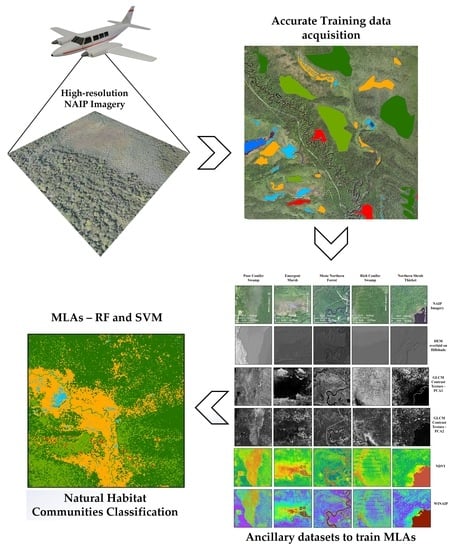
:Remote sensing technology has been used widely in mapping forest and wetland communities, primarily with moderate spatial resolution imagery and traditional classification techniques. The success of these mapping efforts varies widely. The natural communities of the Laurentian Mixed Forest are an important component of Upper Great Lakes ecosystems. Mapping and monitoring these communities using high spatial resolution imagery benefits resource management, conservation and restoration efforts. This study developed a robust classification approach to delineate natural habitat communities utilizing multispectral high-resolution (60 cm) National Agriculture Imagery Program (NAIP) imagery data. For accurate training set delineation, NAIP imagery, soils data and spectral enhancement techniques such as principal component analysis (PCA) and independent component analysis (ICA) were integrated. The study evaluated the importance of biogeophysical parameters such as topography, soil characteristics and gray level co-occurrence matrix (GLCM) textures, together with the normalized difference vegetation index (NDVI) and NAIP water index (WINAIP) spectral indices, using the joint mutual information maximization (JMIM) feature selection method and various machine learning algorithms (MLAs) to accurately map the natural habitat communities. Individual habitat community classification user’s accuracies (UA) ranged from 60 to 100%. An overall accuracy (OA) of 79.45% (kappa coefficient (k): 0.75) with random forest (RF) and an OA of 75.85% (k: 0.70) with support vector machine (SVM) were achieved. The analysis showed that the use of the biogeophysical ancillary data layers was critical to improve interclass separation and classification accuracy. Utilizing widely available free high-resolution NAIP imagery coupled with an integrated classification approach using MLAs, fine-scale natural habitat communities were successfully delineated in a spatially and spectrally complex Laurentian Mixed Forest environment.
1. Introduction
An ecosystem is defined as “a community of organisms and their physical environment interacting as an ecological unit” [1]. Land cover grouped into types and systems by resource managers led Arthur Tansley [2] to coin the term “ecosystem”. Ecosystems with spatially related features are considered higher-order, larger-scale ecosystems, referred to as “macroecosystems” [3]. When ecosystems are viewed as macroscale patterns, they can be divided into ecoregions [4]. The term “ecoregion” was first proposed by Orie Loucks [5], a Canadian forest researcher. Ecoregions play an important role in resource conservation and management by enabling consideration of the natural process and patterns of communities which provide ecosystem sustainability in a particular region [6]. Many different factors (vegetation, soils, spatial and temporal scales, landform and bedrock geology) are utilized to classify these systems, and numerous ecological classification schemes exist. Spatial and temporal dimensions of ecosystem integrity can be addressed using scale (level of detail) and a hierarchical structure approach [7]. Various geographic ordering schemes were developed by Bailey [3,6] to identify and delineate ecoregion boundaries. Additionally, having a hierarchical classification scheme allows ecosystems to be presented at different spatial scales [8,9]. A holistic ecological framework was introduced by Rowe and Barnes [9,10], using a landscape ecosystem or geo-ecosystem approach that incorporates factors such as climate, landforms, soil characteristics, hydrology and biota. An example of a widely used hierarchical classification scheme for wetlands and deep-water habitats for the United States was developed by Cowardin [11]. It divides ecological taxa into hierarchal systems or subsystems to provide mapping uniformity across the United States.
Selecting or developing an appropriate ecological classification scheme is critical for the classification to be useful for the end user. There are numerous existing classification schemes [8,10,11,12], and selection of an inappropriate scheme can limit the end product’s accuracy and utility. To classify a landscape, whether in situ or using remotely sensed data, it is important to have a classification scheme which reduces or eliminates confusion between various landscape features requiring separation [13]. Traditionally, many resource management agencies (federal, state and private) use field-sampled regional vegetation classes focusing on the dominant vegetation species while ignoring associated plants, animals and other organisms which are repeatedly found under similar environmental conditions [14], focusing on describing native ecosystem types minimally impacted by anthropogenic activities [12]. For this study, the hierarchical classification framework of Cohen et al. [12] was utilized. “Natural Communities of Michigan: Classification and Description”, published by the Michigan Natural Features Inventory (MNFI), provides detailed information on separating Michigan’s complex landscape into understandable and describable groups called natural habitat communities. The foundation of this classification is based on the work completed by Chapman [15] and first published by Kost et al. [16]. It is important to understand the difference between a plant community, such as the ones used in the national land cover classification [17], and a natural habitat community [12]. The latter differs from other hierarchical classification schemes in that Cohen et al. [12] regard such a community as “an assemblage of interacting plants, animals, and other organisms that repeatedly occur under similar environmental conditions across the landscape and are predominantly structured by natural processes rather than modern anthropogenic disturbances”.
Along with the classification scheme, it is important to choose appropriate field collection methods and data sources. Commonly used field methods for data collection (e.g., collecting location points via global navigation satellite systems (GNSS) and vegetation sampling) are labor intensive, costly and time consuming. Sampling is confined to small areas due to limited access and safety concerns [18]. With technical advances in geospatial technology, an alternative and/or complementary approach to traditional field data collection techniques is available. Remotely sensed imagery provides a practical, economical approach to monitor and measure biogeophysical factors. Hence, it is efficient for large-area monitoring [19,20,21]. Satellite imagery from multispectral and hyperspectral sensors (Landsat, Sentinel, SPOT, MODIS, and HyMap) as well as LiDAR and RADAR data have been extensively used for land cover mapping at various scales [17,22,23,24,25,26,27,28,29] Fine-scale mapping is critical to locate and map endangered habitats, particularly with escalating global climate change impacts. Hence, high spatial resolution imagery, such as that of the National Agriculture Imagery Program (NAIP), is important. The NAIP program is managed by the Aerial Photography Field Office (APFO) of the United States Department of Agriculture (USDA). It has 8-bit radiometric and 60 cm spatial resolutions, with four spectral bands (near infrared (NIR), red, green and blue). NAIP data are nominally cloud-free and widely available at no cost [30]. They have been used for wetland mapping, land cover classification, forest-cover-type mapping, forest health monitoring and other resource management projects [31,32,33].
Additionally, selection of an appropriate classification algorithm is dependent on the image spatial resolution, chosen classification scheme and landscape complexity. In the last two decades, the remote sensing community has steadily increased its use of machine learning (ML) classification techniques [23,34,35,36,37,38], as the limitations of traditional parametric classification techniques such as maximum likelihood are realized. Machine learning algorithms (MLAs) use a nonparametric approach to model and classify data, and do not require normally distributed data [39]. Numerous land use/cover classification studies have shown the advantages of using MLAs such as random forest (RF) and support vector machine (SVM) [23,40,41,42,43]. MLAs were utilized in the classification of the 2001 National Land Cover Database (NLCD) [17]. They have also been used with NAIP imagery for accurate land cover classification [30,44].
Factors such as training set quality, selection of the optimum number of ancillary datasets and training parameters affect the performance of MLAs [39,45]. Poor-quality training data impact the accuracy of MLAs. The use of image transformations such as principal component analysis (PCA) and independent components analysis (ICA) reduces or eliminates redundant spectral information. Ancillary data such as landform, soil characteristics, hydrography and expert knowledge of the study area are important to create high-quality training sets. The use of valid ancillary datasets also plays a crucial role in the classification of vegetation communities. It is important to understand which ancillary datasets are impacting classification accuracies. Feature selection methods identify the best ancillary data before executing MLAs and reduce the complexity of the method (e.g., the “Hughes phenomenon” [46]) and overall computational time [39]. Researchers have shown the usefulness of feature selection methods and multiple ancillary datasets to improve land cover classification [30,44,47,48].
Northern forests of the Upper Midwest are part of the Laurentian Mixed Forest (LNF) which is an extremely complex landscape in terms of geomorphology and vegetation, due to extensive regional glaciation [49,50]. This has led to unique and complex landforms that dictate the topography, soil characteristics, hydrography and vegetation communities [49]. The LMF occurs between the boreal forest and the broadleaf deciduous forest transition zones [51]. Although there are a number of completed studies using grouped species classifications in this region [14,52,53,54], to the best of our knowledge no study has been performed using a natural-habitat-community-level classification scheme [12] with MLAs.
Hence, the goal of this study was to develop a robust methodological classification approach to identify and accurately classify spectrally similar natural habitat communities of the complex Laurentian Mixed Forest region using the MNFI natural habitat communities classification scheme [12]. To achieve this, we proposed an integrated approach of spectral enhancement techniques coupled with elevation, soils and field data to obtain accurate training data. Classification accuracies were compared between two commonly used MLAs, RF and SVM, using various ancillary data derived from feature selection methods, along with the high spatial resolution NAIP dataset.
2. Study Area, Data and Methods
2.1. Study Area
The study site (Figure 1), is the Sturgeon River watershed (HU5 Id 20207).
(45°50′27″N, 86°40′30″W) located in the western half of the Hiawatha National Forest, adjacent to the head of Big Bay de Noc. The study area encompasses approximately 3151 ha (77,861 ac) and contains a wide variety of natural habitat communities. Dominant vegetation is composed of upland and lowland deciduous, conifer and mixed forest types as well as palustrine wetlands [55]. The influence of the Great Lakes and various landforms creates distinct climatic zones across the area with summer temperatures ranging from 22 °C (71 °F) near the Great Lakes shoreline to a warmer 27 to 29 °C (81 to 85 °F) inland. Winter temperatures range from an average high of −2 °C (28 °F) to an average low of −11 °C (13 °F). Winters are long and snowy, with average snowfall of 142 cm (56 inches) along the Lakes Michigan and Huron shorelines, to 554 cm (218 inches) near Lake Superior. The study area is part of a glacial lake plain and is a nearly level lake plain that was covered with water from the glacial Lake Algonquin. The soils on the landform are derived from predominantly sandy lacustrine deposits [49,56]. Soil drainage classes range from poorly to excessively drained, and soil pH ranges from neutral to extremely acidic. The area contains numerous wetlands with a complex hydrography.
2.2. Imagery
The National Agriculture Imagery Program (NAIP) collects data during the active growing season, also known as “leaf-on” imagery, which is needed for habitat classification. The four-band (red, green, blue and near-infrared) aerial imagery was acquired at approximately 16,000 feet above ground level (AGL) with a Leica ADS100 airborne digital sensor (Leica Geosystems). The image has a spatial resolution of 60 cm with 8-bit radiometric resolution. The spectral range of the 4 bands ranges between 435 and 882 nm (Table 1). The data were preprocessed by the contractor to reduce radiometric and geometric distortions. NAIP imagery tiles dated 25 July 2018 and 11 August 2018 were downloaded from the United States Geological Service (USGS) EarthExplorer website (https://earthexplorer.usgs.gov/, accessed on 14 July 2021). A LiDAR-derived 1 m digital elevation model (DEM) was obtained from the Natural Resources Conservation Service (NRCS). All datasets were registered to the Universal Transverse Mercator (UTM), Zone 16 North, North American Datum of 1983 (NAD83). The spatial resolution for all the datasets is 60 cm. Where resampling was required, the data were reprojected using a two-dimensional affine coordinate transformation using nearest-neighbor resampling, with a fundamental vertical accuracy of ±24.5 cm, meeting all FGDC (Federal Geographic Data Committee) standards.
ERDAS IMAGINE® 2020 (https://www.hexagongeospatial.com/products/power-portfolio/erdas-imagine, accessed on 14 July 2021) and ArcGIS Pro 2.7 (https://www.esri.com/en-us/store/arcgis-pro, accessed on 14 July 2021) were used for image transformation. IMAGINE’s Spatial Model Editor toolbox was used to generate the normalized vegetation index (NDVI) and a modified water index (WINAIP), as well as the gray level co-occurrence matrix (GLCM) textures, aspect and slope (%). ArcGIS Pro tools were used to generate random points (Create Random Points) and to extract multi raster values (Extract Multi Values to Points). The “caret” package [57] of the R programming language [58] was used for MLA implementation.
2.3. Methods
2.3.1. Utility of Image Transformations
Multiple workflows have been developed by the remote sensing community for delineating and mapping vegetation. They are dependent on environmental factors (e.g., soil characteristics (drainage, slope, pH), hydrography, landform and climatic conditions) [59], as well as field collected data, expert image interpretation (manual and computer assisted) and an appropriate classification scheme [11,12,47,48,60,61,62]. The delineation and classification workflow used in this study is presented in Figure 2. Inter-class spectral variability is important to differentiate natural communities. However, locally high variance occurs not only due to changes in vegetation but also due to site conditions and the high spatial resolution of the imagery [63]. When selecting training sets, it is important to understand how these factors influence training set statistics and to generate adequate training data to encompass the variation. Having polygon training sets with well-delineated feature boundaries is critical to generate valid training set point matrices for the machine learning algorithms (MLAs) [39].
To fully utilize spectral reflectance information, and reduce redundant information between bands, an integrated approach to spectral transformation techniques (principal components analysis (PCA) and independent components analysis (ICA)) were utilized. PCA is a widely employed transformation using a linear transformation, and it generates uncorrelated components [64,65]. PCA-derived components have been used to map wetlands vegetation, assess change detection and evaluate vegetation anomalies and identify geological features [66,67,68,69,70]. PCA uses second-order statistics and assumes the data are normally distributed and correlated. PCA has been utilized since the launch of the Landsat 2 Multispectral Scanner which consisted of 4 bands [71]. ICA considers higher-order statistics, and each transformed component is considered to be non-Gaussian [72]. ICA has been shown to identify details in an image even when the feature occupies a small area [73]. However, it has not been extensively used in vegetation and land use/cover classification [70,74,75,76]. Both PCA and ICA were used to draw accurate training classes for the MLA. The components of the PCA transformation were not used in the classification process, as components 3 and 4 contained information critical to delineating the emergent marsh natural habitat communities.
2.3.2. Vegetation and Moisture Indices
Spectral indices have been used extensively to evaluate, monitor and map vegetation both qualitatively and quantitatively [77]. Two spectral indices, the normalized vegetation index (NDVI) and a modified water index (WINAIP), were derived from the NAIP bands. NDVI indicates the biomass abundance and vigor, as well as differentiating vegetation from non-vegetated areas [78,79]. NDVI was generated using NAIP bands 4 (NIR) and 1 (red). The WorldView water index (WV-WI) was proposed by Wolf [80] and uses WorldView satellite band combinations of coastal blue (425 nm) and the second near-infrared channel (NIR2) (950 nm). Previous water indices for satellite imagery were based on NDWI [81] which used NIR and short-wave infrared (SWIR) channels. Based on Wolf’s index, a custom water index was developed for this study by replacing the coastal blue band (425 nm) band with NAIP blue (435 nm) and the NIR2 (950 nm) band with NAIP NIR (882 nm). The modified index is referred to as the WINAIP.
2.3.3. Texture
Plant communities often share similar spectral reflectance characteristics, which leads to confusion and misclassification. In such scenarios, texture differences may be useful, even critical, for correct classification. A gray level co-occurrence matrix (GLCM), originally referred to as a “gray-tone spatial dependence matrix” by Haralick et al. [82], uses second-order metrics to analyze relationships between pairs of pixels and computes both angular relationships and directionality to measure the spectral and physical distance between two neighboring pixels [83]. GLCM texture analysis has been used in numerous studies to classify various features including urban areas, forests, agriculture and wetlands [61,82,83,84].
The GLCM texture was calculated from the first and second NAIP PCA components. These components explained 94% (component 1) to 96.74% (components 1 and 2) of the variability in the image. Three different GLCM measures of texture (contrast, entropy and standard deviation) were calculated with PCAs 1 and 2. GLCM was performed in ERDAS IMAGINE (Hexagon Geospatial, 2020), with a grayscale level of 32 and 3 × 3, 5 × 5 and 7 × 7 processing windows. Two different Euclidean geometry XY offsets (2, 2 and 2, −2) were used. The derived means from the texture measures were used in the classification.
2.3.4. Topographical Characteristics
At fine scales, natural habitat communities are controlled by soils, local topography, lake effect climate zones and, in some instances, past disturbances such as fire and windthrow. Extensive glaciation in the Upper Midwest has created a wide variety of surficial geologic features. These features are made up of interacting landform patterns, which have been described [56,85] as combinations of “relief-topography (surface shape) and geological parent material”. Rowe [10,56,86] stated that “repetitive patterns in vegetation can be traced directly to repetitive patterns of topography associated with specific types of surficial material of landforms”. Drawing on this body of research, a 1 m DEM generated from LiDAR imagery collected in 2015 helped identify important topographic features with high positional accuracy. The DEM was downloaded from the National Resources Conservation Service. Hillshade (multi-directional oblique weighted—MDOW), aspect and slope (%) were generated from the DEM. Aspect and slope were evaluated as input ancillary data into the MLAs and hillshade aided in manual training set delineation.
2.3.5. Selection of Input Ancillary Data Layers
When imagery alone cannot adequately classify the data, the incorporation of ancillary data is important. Once ancillary data layers are selected, understanding their contribution towards classification is important [87], with the goal of optimizing and creating an accurate classification. Variable or ancillary data selection has been used in many applications including data mining and machine learning, network anomaly detection, natural language processing, bioinformatics and image processing [87]. There are many different feature selection methods available [88].
In this study, joint mutual information maximization (JMIM) [89], a filter-based variable selection method, was implemented in R using the “praznik” package [90]. This method uses “mutual information” and “maximum of the minimum” criteria to calculate the contribution of each input variable. This method evaluates each variable’s importance. The JMIM method was performed prior to running the MLA classification. Variables with higher JMIM values were used as ancillary data inputs. Along with the JMIM method, the “varImp” function was used [89] from the “caret” package [57,91], which evaluates the implemented MLA and identifies the best ancillary data layers for improving the classification [88,91]. The varImp method is implemented after the RF classification is performed. The scores produced for each variable helped select various variable combinations for the MLAs classifications.
Based on joint mutual information maximization (JMIM) and “varImp” scores, the following variables were used as inputs in the machine learning algorithms (MLAs):
- Four bands of NAIP imagery;
- Elevation from DEM;
- Contrast texture (C1*7) calculated from PC1 (7 × 7) moving window, C2*7 calculated from PC2 (7 × 7) moving window;
- Normalized vegetation index (NDVI);
- Modified water index (WINAIP) derived from NAIP imagery.
Feature selection methods have been primarily used in geology applications to reduce the complexity of the dataset where there are large numbers of bands (i.e., hyperspectral data) [70]. In this study, both feature selection methods were implemented. However, as this is an uncommon approach for natural resource applications [92,93,94], various combinations of the ancillary data were also manually selected and evaluated, and listed in the results section.
2.3.6. Collection of Training Samples
An adequate number of training samples is crucial to achieve optimum classification results. As a “rule of thumb” in ML, the number of training samples should be 10 times (preferably 100 times) the total number of variables [39,95]. How the training samples are selected also plays a crucial role and requires expert knowledge of the spectral and spatial variation within and between the natural communities [13]. Additionally, the choice of classification algorithm, the number of input variables and the spatial extent of each natural habitat community influences the number of training samples required [39,96]. Researchers have noted that large and accurate training datasets are preferable, regardless of the MLA used [39,97,98]. Training samples were generated within manually delineated training set polygons (Figure 3) using stratified random sampling in ArcMap 10.7.1, with a minimum of 5 m distance between points. Different spectral enhancement techniques (PCA, ICA), soils, elevation data and ground truth data were utilized to delineate the training polygons. Table 2 presents the natural communities within the study area and the number of training and test points collected for each. The points were assigned natural habitat community class names and IDs. Using the X and Y locations of the training sample points, pixel values for the NAIP imagery and the ancillary data layers were extracted for use in the MLAs.
2.3.7. Utilization of MLAs for Natural Communities Classification
The training samples derived from the input ancillary data layers were used to train both random forest (RF) and support vector machine (SVM). Parameter optimization, validation and accuracy assessment were performed for both algorithms. The “caret” package [57] available in the “R” programming language was used to implement the MLAs. RF and SVM classifiers are discussed briefly below.
2.3.8. Random Forest
RF is an ensemble classifier method developed by Brieman [99], which uses a set of nonparametric classification and regression tree (CART) rules to make predictions [100]. Decision trees (DTs) are generated using the values of a random vector sampled independently from the input vector and distributed equally among all the trees in the forest [35,38,101,102]. The algorithm then uses the majority of votes from the tree’s assemblages and assigns that value to each of the unknown vectors [39,47]. Random forest works with a “bagging” (or bootstrap aggregating) approach, which generates training datasets by randomly drawing replacements for the original training set for each selected feature/feature combination [38,99,103]. RF uses two thirds of the data to train the trees and the remaining one third of the data to provide an independent estimate of overall accuracy (OA) [34,39]. The classifier is computationally efficient but can be prone to overfitting [104,105]. The forest can grow to a user-defined largest number of trees (Ntree) by optimizing the number of RF-created trees exhibiting high variance and low bias [34,99]. The mtry parameter controls the number of variables randomly selected at each split in the tree-building process and has a sensitive influence on RF’s performance. It can be adjusted if needed, as part of the tuning process [106,107]. RF’s advantages include its ability to work with spatially large, complex datasets with correlated variables, to rank variable importance and to improve classification accuracies [39,99]. We used the default parameters provided with the “rf” method in the caret package and used “center” and “scale” to standardize the ancillary data [57,108]. RF tends to work robustly without optimization parameters [39].
2.3.9. Support Vector Machine
SVM is a supervised machine learning algorithm developed by Vapnik [109], based on statistical learning theory. The classifier is inherently binary and tries to identify a boundary or a hyperplane which separates two classes that are closest in the feature space. The hyperplanes associated with the class are parallel to the optimal separating hyperplane and the samples located on these hyperplanes are called support vectors [109,110].
However, in the real world, data distributions are often non-linear and noisy, and may not be easily separated, which promotes overfitting. Projecting the input data to a higher dimension feature space helps overcome this issue, assuming that a linear boundary exists in the higher dimensional feature space [39,111]. If a linear higher dimensional feature space does not exist, a kernel function can be used, and for this study a radial basis function (RBF) kernel was used [112]. We used the default “svmRadial” method from the caret package [57]. SVM contains two important model parameters: “cost” (C) and “sigma” (σ). Higher C values can lead to a more complex decision boundary and less generalization [39], whereas a higher σ affects the overall shape of the separating hyperplane and may influence overall accuracy. The “caret” package estimates approximate values for the cost and σ parameters directly [57,108,113]. RBF parameters are determined by a grid search algorithm using an m-fold cross-validation (m-FCV) approach. The grid search method tests different pairs of parameters, and the one with higher cross-validation accuracy is selected [114]. Centering and scaling were performed to standardize the ancillary data [57,108].
2.3.10. Accuracy Assessment and Classification Differences
Thematic accuracy assessment is an important component in evaluating the “correctness” of a classification. Products with low accuracy have limited or no utility to the end user, as they are composed of misinformation. Stratified random sampling was selected for the accuracy assessment points. This sampling approach ensures unbiased sample selection and adequate sampling for each habitat, since a minimum number of samples is specified for each class [117,118]. Using the methodologies developed by Congalton and Green [13], error matrixes, overall accuracies, kappa and Z-scores with 95% confidence limits were calculated.
Differences in the output classifications occur, as the MLA algorithms do not process the data the same way. Processing differences do create different end products. Differences between the two MLA outputs were assessed using ArcGIS Pro 2.7.
2.3.11. Classification Post-Processing
Classified data, including the natural habitat community classifications resulting from the MLAs, manifested a “salt and pepper” appearance due to the spectral variability encountered by the classifier [66,119]. A single pixel, due to its small area, doesn’t provide useful information to a resource manager and may have little or no relation to the actual mapping of a natural habitat community [13,120,121]. It is common practice to remove noise using a majority filter and a specified window size [66] to create homogenous polygons suitable for accuracy assessment. To make the natural habitat community classes easily identifiable, and the final map more useful to the end user, we applied a 7 × 7 moving window majority filter.
3. Results
Natural habitat community classification was evaluated using RF and SVM with various input ancillary datasets including NAIP spectral bands, topographical layers, textural measures and spectral indices, to classify the natural communities (Table 3). The training and testing datasets were split 75% and 25%. The appropriateness of the input datasets was evaluated based on the overall accuracy (OA) and kappa (k) of the test samples (5801 pixels). OA indicates the ratio between the total number of pixels and the total number of accurately classified pixels, and the k (kappa) is a measure of the agreement between the accurately classified data and the reference data [13]. Along with OA and k, the UA and PA for each community class were also evaluated. User’s accuracy (UA) and producer’s accuracy (PA) show the accuracy of each community class, as described by Congalton [13]. UA and PA show the commission and omission errors of individual classes, respectively. Z-scores with a 95% CI were also evaluated. Along with these, a difference map was generated to evaluate the classifier differences.
3.1. Ancillary Data and Feature Selection Methods
A total of 19 ancillary datasets (Figure 4) were evaluated in this study. The contrast texture image provided the most detailed information compared to entropy and SD. Hence, two more images were generated using 3 × 3 and 5 × 5 moving windows to evaluate impact of window size on the natural habitat community MLA classifications. JMIM and varImp scores were calculated for all of these input ancillary datasets from highest to lowest scores. Classifications using RF and SVM were generated using all possible combinations of the above-mentioned ancillary data layers (Table 3) to verify the robustness of the feature selection methods. Ancillary data layers which had lower scores in the feature selection method (Figure 4) showed similarly poor performance in the MLA classifications (Table 3 and Table 4).
3.2. Classifications Results
The lowest accuracy occurred when only the National Agriculture Imagery Program (NAIP) bands were used for classification and supports the need for ancillary data incorporation. Using only the four multispectral NAIP bands (Input 1) led to a low OA (56.02%, k = 0.46) with RF and with SVM (OA = 59.01%, k = 0.49) (Table 3). The addition of slope, aspect, normalized difference vegetation index (NDVI), NAIP water index (WINAIP) and texture improved the OA. The highest classification accuracies included those using all the input ancillary data (Input 3) and those using a combination of derived indices and textures. Table 3 and Table 4 shows the overall accuracy (OA), kappa (k) and confidence intervals (CI) and other supporting statistics the natural habitat community classifications derived from various input variable combinations. RF has OAs and associated k values ranging from 56.02 % (k = 0.46) for Input 1 to 79.96% (k = 0.75) for Input 3. SVM values were between an OA of 59.01% (k = 0.49) for Input 1 and 75.85% (k = 0.70) for Input 4. Using Cohen’s categorization of kappa value ranges, the classifications from Inputs 2, 3 and 4 (Table 4) show substantial agreement.
Incorporating the DEM with the NAIP bands provided a significant improvement in OA (12 to 17% increase) regardless of the MLA. Using slope and aspect with the NAIP bands did not significantly improve the OA. Similarly, vegetation and water indices did not differ significantly compared to those using only the four NAIP bands. When all variables (Table 3), including the four NAIP bands, three topographic layers, ten texture layers and two indices were used, the OA improved to almost 80% for RF and 74% for SVM (Table 3). Figure 5 shows the graphical representation of OA and k for NAIP bands, all ancillary dataset and the final classification approach. Input 4 ancillary data layers were used for the final classification (Figure 6 and Figure 7), giving 79.45% OA for RF and 75.85% for SVM. Between Input 3, which used nineteen ancillary data layers, and Input 4, which used only nine ancillary data layers, no significant statistical differences were observed (Table 3 and Table 4).
Z-scores with a 95% confidence limit were calculated for all k values and are shown in Table 4. The scores for each classification, regardless of input variable combination, show the classification to be meaningful and significantly better than a random classification. Pairwise Z-scores are also presented in Table 4. The scores indicate that all of the classification results for RF and SVM with the same input variables were not statistically different, as all have an absolute value < 1.96.
Figure 6 and Figure 7 present the final classification results from Input 4 data (Table 3) for RF and SVM. There are five natural habitat community classes (Figure 6 and Figure 7), with four non-habitat community classes (Open Land, Impervious, Inland Lake and Open Water) which are not considered natural habitats under the current classification scheme but reflect human influences on the landscape, such as agricultural/open land and roads, and must be included. Input 3 led to a slightly higher OA, but this was not statistically significant (Z-score) compared to Input 4, which had fewer variables. Fewer variables shorten the computing time, which is an important consideration for classification of large areas. However, the kappa and Z-score are only two measures of classification quality; they only consider the overall classification and not the accuracies of the individual natural habitat community classes.
Table 5 presents the error matrix, including user’s accuracies (UA) and producer’s accuracies (PA) for the final RF and SVM natural habitat communities classification. A total of 5,801 randomly selected ground truth points were used for the accuracy assessment (Table 5). Each natural habitat community class had at least the minimum number points to create a 95% confidence interval and was based on the percentage area of each class with respect to the total area.
The PAs and UAs calculations show the accuracies of the natural habitat communities can be split into two groups: those with accuracies above 85% and those with accuracies between 60 and 75% (Table 5). Open Land (OL), Emergent Marsh (EM), Mesic Northern Forest (MNF), Inland Lake (IL), Open Water (OW) and Impervious Surface (IS) have PAs between 84 and 100%. Rich Conifer Swamp (RCS), Poor Conifer Swamp (PCS) and Northern Shrub Thicket (NST) have PAs between 41 and 81%. These lower PA accuracies can be explained by the presence of speckled alder (Alnus incana), red osier dogwood (Cornus sericea), white pine (Pinus strobus) and red maple (Acer rubrum) across all three communities [12]. Sphagnum mosses (Sphagnum spp.), bunchberry (Cornus canadensis), balsam fir (Abies balsamea), paper birch (Betula papyrifera), black spruce (Picea mariana), huckleberry (Gaylussacia baccata) and sensitive fern (Onoclea sensibilis) are found in both Rich and Poor Conifer Swamp communities [12]. The presence of these species in both communities contributes to the lower UA and PA (Table 5). Also contributing to the Northern Shrub Thicket’s lower UA and PA was misclassification between it and Emergent Marsh. This is due to large areas of spatial intermixing of the two communities. Similar observations were made from the classifier difference map (Figure 8), where majority of confusion with the SVM classification was observed in RCS, PCS and NST natural habitat communities. Areas in red show where differences in the natural habitat communities occur between the MLAs. Otherwise, the classification results were in agreement.
4. Discussion
4.1. Feature Selection and Imprtance of Ancillary Datasets
Ancillary datasets such as NAIP (National Agriculture Imagery Program) multispectral bands, DEM, aspect, slope, spectral indices and PC1- and PC2-based texture layers were selected by implementing the feature selection method. The utility of these input datasets was determined and compared for the automated MLAs. The ancillary data were selected not only based on the variables’ importance but also on the OA and k values as well. Both of the feature selection methods (i.e., JMIM and varImp) proved to be important for observing differences in ancillary data contributions to the MLA accuracies (Figure 4a,b).
The JMIM (Figure 4a) scores are independent of the classification algorithm and are generated prior to running the MLAs. The ranking serves as a guide to the potential contribution of the variables and assists in initial variable selection. This is important when there are numerous inputs to choose from. By contrast, the varImp (Figure 4b) ranks the importance of input variables only for random forest and is generated after the classification is performed. This ranking allows confirmation of the input variable’s importance and validates the original selection of the input variables. The order of variable listing is not expected to be the same when calculated at different points in the workflow. However, the first nine listed variable rankings are closely similar for both feature selection approaches. The approach also confirms the lower contribution of the useful information of certain variables such as slope and aspect.
Regarding spectral indices, both NDVI and WINAIP were helpful in improving the accuracies. NDVI was critical for calculating the green biomass present in the area, and it assisted in discriminating Mesic Northern Forest from Northern Shrub Thicket. For WINAIP, even though the NAIP bandwidths did not match as the WV-WI bandwidths, initial results showed that the modified index contributed to differentiating standing waterbodies, emergent marsh and shadows efficiently. Of the three calculated GLCM texture measures, contrast provided the most useful information for classification. Emergent Marsh, Northern Shrub Thicket and Water had smooth textures and hence low mean contrast values, whereas Mesic Northern Forest, and Rich and Poor Conifer Swamps had high mean contrast values, due to a rough texture. Average mean contrast values in the study area ranged from 0 to 285. To determine the best texture window size and evaluate finer-scale changes in texture, three different moving window sizes were evaluated (3 × 3, 5 × 5 and 7 × 7) using contrast. The largest window size (7 × 7) performed well for entropy and standard deviation (Figure 4a,b) providing unique information. However, contrast texture outperformed both entropy and standard deviation in differentiating natural habitat communities. Only the first two PCA components were used to generate GLCM texture. PCs 1 and 2 explained 96.74% of the variability in the original NAIP data. The feature selection methods (JMIM and varImp) may not necessarily improve accuracy, but they helped to reduce the model complexity by allowing a selection of variables which contributed the greatest amount of information to the classification.
4.2. MLAs Classifier Performance
Overall, random forest (RF) outperformed support vector machine (SVM), including giving the classification with the highest overall accuracy (OA) and kappa value (k). In comparison to the SVM model, the RF model was more robust at handling a higher number of ancillary datasets (Table 3). Our observation showed that the DEM can be considered as important ancillary data in classifying and increasing the model accuracy for the community types. The smallest changes in elevation reflect a variation in soil types and drainage patterns which can influence the natural habitat community of the area [47]. The model which was used for the final classification (Input 4), showed a 6.36% increase in OA for RF and 4.64% for SVM, compared to Input 2 where we only used two ancillary data layers. Therefore, users who wish to increase the model OA in similar environmental conditions should consider using elevation as ancillary data, along with texture and spectral indices. Of the three GLCM textures, contrast proved to be the most useful, followed by entropy and standard deviation (Figure 4).
Both RF and SVM showed major confusion between RCS, PCS and NST classes. RCS and PCS have a variety of tree species of similar types, which can cause confusion in the classification. NST is another community class which shares similar vegetation types with RCS and PCS, and also showed lower UA and PA (Figure 9a,b). Due to the close spectral similarities between these classes, they have a lower UA and PA overall compared to other classes (Figure 9a,b). Classes with higher spectral dissimilarity showed maximum accuracy (i.e., OL, EM, MNF and IL) and vice versa. Considering the overall UA and PA for the community classes, we see that in general, RF (Figure 9a) performed better than SVM (Figure 9b). For example, all five natural habitat community classes (EM, RCS, PCS, NST and MNF) showed better or similar UA and PA values compared to SVM (Figure 9a,b).
The final classified maps from the RF (Figure 6) and SVM (Figure 7) algorithms show that RF delineated the natural community boundaries better than SVM. Figure 8 shows the classification difference map between RF and SVM. Areas of disagreement are shown in red. Most of the confusion occurs between Rich Conifer Swamp, Poor Conifer Swamp and Northern Shrub Thicket, and there are errors of both commission and omission in the accuracy assessment matrix (Table 5). These areas occur along the glacial lake shoreline (west side of study area), in the riparian area of the Sturgeon River (center of study area) and on moraines (southeast corner of study area). Areas such as Open Land, Open Water, Impervious Surface and Emergent Marsh show agreement across the landscape for both MLAs. Higher confusion was observed in the SVM accuracy assessment matrix, resulting in lower PA and UA compared to RF. It is important also to visually assess the final classifications, not just the matrices, to fully understand the MLA performance.
4.3. Overall Performance of MLAs for Natural Habitat Communities Classification
The classification results are similar to the outcomes of previous studies where RF outperformed the SVM model. The SVM model tends to work better with a smaller number of classes, whereas RF can work with a larger number of classes [39]. In the past, Rodriguz-Galiano et al. [22,23] successfully used RF to map and classify 14 classes using Landsat TM and ancillary datasets, with a high OA. Berhane et al. [47] discriminated 22 wetland classes and achieved the highest OA using RF with WorldView-2 multispectral data, along with various ancillary data. Higher accuracies with RF classifications compared to SVM classifications were also observed by Adam et al. [122] for land-use/cover classification. Hayes et al. [44] used the RF classifier to successfully classify nine landcover classes using NAIP bands and additional ancillary data such as spectral indices, elevation data, texture, etc. Land cover classification is common in the remote sensing community, but this is the first time the natural communities of Michigan classification system [12] has been used to classify a complex Laurentian Mixed Forest system at the natural habitat community level.
4.4. Importance of Reference Vegetation Map
The color infrared (CIR) combination (R:4, G:3, B:2) of high-resolution multispectral data and high spectral contrast from the feature extraction techniques (PCA, ICA) helped differentiate the natural habitat community types. Ancillary data such as the soils map (soil moisture, pH, drainage), as well as prior fieldwork and knowledge of the study site contributed important information. Figure 3 shows the reference natural habitat community map, where nine different classes were delineated, including five community types (Table 2). The component combination (R:4, G:3, B:2) from PCA and ICA (Figure 10) transformation showed outline boundaries between forest, marsh, swamps, thickets, open land and water groups. Figure 10 shows how the differences in texture from the five natural habitat communities were enhanced and visualized using the PCA and ICA components, compared to the original NAIP imagery. This distinction between different natural habitat communities permits more accurate boundary delineation for better training data, compared with traditional maps, which are drawn at larger scale and have lower spatial resolution (i.e., NWI and NLCD maps). Both RF and SVM models require good training data in order to perform well [39].
4.5. Impact of Number of Training Samples and Quality of Sample Data on MLAs
The reference vegetation map was used to generate random training points for the nine classes within delineated polygons. Data from field validation, expert knowledge and a limited, very high spatial resolution UAS dataset [55] for the area provided a reliable and accurate reference map. The training points (total number = 23,214) were divided into groups of 75% and 25%, respectively, for the training and testing datasets (Table 2). Potentially, an increase in the number of training and testing points could achieve higher classification accuracies. For example, this study used a minimum distance of 5 m between the randomly generated points for each community class. If the distance was decreased to 3 m, it would allow a greater number of points for training and testing. Researchers have shown in the past that training sample size can play a crucial role in the classification accuracies for supervised machine learning algorithms [39,96]. The required number of training data points also depends on the classification algorithm, number of ancillary datasets and the size and complexity of the study area [96].
4.6. Validation of Classified Community Vegetation Map Using Field Data and Expert Observation
The study area is in a remote rural location where land use and cover changes are minimal. Parts of the study area are protected from exploitation and development. There is limited access, which constrains field verification due to a lack of roads and a complex network of land ownership where most private lands cannot be traversed, and many of the natural communities also prohibit ground truthing for safety reasons. Where possible, ground surveys were conducted during the summers of 2018, 2019 and 2020. However, field work in 2020 and 2021 was severely curtailed due to the COVID-19 pandemic. Additional reference data were collected by observations made by an expert interpreter of the NAIP imagery outside of the reference area polygons, as well as using United States Forest Service (USFS) stand compartment maps [53]. This was the first time the Laurentian Mixed Forest of the Hiawatha National Forest (HNF) has been classified using the natural communities classification system [12]; as a result it was not possible to directly compare it to any previously available maps.
4.7. Future Work
Future research will involve assessing the robustness of this classification approach using other study sites with different natural communities, varying landforms and soil conditions. Consideration will be given to mapping spatially larger areas such as an entire watershed, as well as looking at smaller areas with limited natural communities such as fens. In Michigan, there are five different fen communities [12], and they can exist adjacent to each other. Being able to accurately map natural communities at different scales is important, in order to understand, describe, document and restore natural habitat community diversity.
Consideration must also be given to what classes should be incorporated into the classification for areas influenced by modern anthropogenic distributions such as agriculture, mining and development. Non-natural habitat community classes were added as needed in this study. This is not a robust approach. These classes should be well defined, mutually exclusive and hierarchical in structure.
5. Conclusions
Community classification for Laurentian Mixed Forest is challenging, due to the complexity of the landscape. In this paper, for the first time, a natural habitat community level classification using an integrated approach of spectral transformation and enhancement techniques, field data, ancillary datasets and MLAs was implemented. Feature selection methods such as JMIM and varImp were used to evaluate the utility of a wide variety of ancillary data including elevation, various measures of texture, and vegetation and soil moisture indices and to guide the selection of the best-performing ancillary data. High-spatial resolution data and machine learning algorithms contributed to a successful and accurate classification.
Five complex natural habitat communities and four non-natural habitat communities were successfully classified. Due to the spectral limitation of the four NAIP bands, the classification showed confusion between similar natural habitat communities (e.g., Rich Conifer Swamp vs. Poor Conifer Swamp vs. Northern Shrub Thicket), with accuracies ranging from 72.55% down to 64.70% (Table 5). Discrimination between Mesic Northern Forest, Emergent Marsh, Impervious, Open Land and Water (Open Water and Inland Lake) had higher accuracies (100% to 89.36%) (Table 5).
RF and SVM both showed promising performance for classifying a complex Laurentian Mixed Forest community. RF outperformed SVM in the final classification results but SVM performed well when there were fewer ancillary datasets. The choice of MLA may vary for users, depending on the site, type of communities being mapped, number of ancillary datasets and quality of the training data. In R, parameter optimization is allowed and can help provide better performance, but the use of optimization parameters may increase the processing times of the classifiers. In this study, we used the default parameters of the classifiers, as they were accurate enough and achieved the desired results. We also believe that using more spectral bands might improve the classification and could help overcome the complexity of the vegetation classes.
Author Contributions
P.B. analyzed the data, designed the study approach, performed the experiments, did field work and wrote the manuscript draft; A.M. wrote the original project proposal, did field work, advised on methodology improvements and revised the manuscript; Y.D. provided comments and revised the manuscript; C.K. helped with methods, and provided comments on methodology and interpreting the results. All authors have read and agreed to the published version of the manuscript.
Funding
This research was funded by the US Forest Service, Hiawatha National Forest (Grant Number 17-PA-11091000-023), The Nature Conservancy (Grant Number R45984) and the College of Forest Resources and Environmental Science.
Data Availability Statement
Not Applicable.
Acknowledgments
We would like to thank the College of Forest Resources and Environmental Science, Michigan Technological University for their support. We also thank Ian Anderson (Chief Product Owner) of Hexagon Geospatial for his crucial help at the beginning of this project, Jim Ozenberger of the Hiawatha National Forest for assistance with field work and Emily Clegg of The Nature Conservancy for providing technical support.
Conflicts of Interest
The authors declare no conflict of interest.
References
- Lincoln, R.J.; Boxshall, G.; Clark, P.F. A Dictionary of Ecology, Evolution and Systematics. Syst. Bot. 1983, 8, 339. [Google Scholar] [CrossRef]
- Tansley, A.G. The Use and Abuse of Vegetational Concepts and Terms. Ecology 1935, 16, 284–307. [Google Scholar] [CrossRef]
- Bailey, R.G. Ecosystem Geography: From Ecoregions to Sites; Springer Science & Business Media: Berlin/Heidelberg, Germany, 2009. [Google Scholar]
- Bailey, R.G. Identifying ecoregion boundaries. Environ. Manag. 2004, 34, S14–S26. [Google Scholar] [CrossRef] [PubMed]
- Loucks, O.L. A forest classification for the Maritime Provinces. Proc. Nova Scotian Inst. Sci. 1962, 25, 1958–1962. [Google Scholar]
- Bailey, R.G. Delineation of ecosystem regions. Environ. Manag. 1983, 7, 365–373. [Google Scholar] [CrossRef] [Green Version]
- King, A.W. Considerations of Scale and Hierarchy. In Ecological Integrity and the Management of Ecosystems; CRC Press: Boca Raton, FL, USA, 2020; pp. 19–45. [Google Scholar] [CrossRef]
- Bailey, R. Ecoregions of the United States (Map); US Department of Agriculture, US Forest Service, Intermountain Region: Ogden, UT, USA, 1976. [Google Scholar]
- Barnes, B.V. The landscape ecosystem approach and conservation of endangered spaces. Endanger. Species Update 1993, 10, 13–19. [Google Scholar]
- Rowe, J.S.; Barnes, B.V. Geo-ecosystems and bio-ecosystems. Bull. Ecol. Soc. Am. 1994, 75, 40–41. [Google Scholar]
- Cowardin, L.M.; Carter, V.; Golet, F.C.; LaRoe, E.T. Classification of Wetlands and Deepwater Habitats of the United States; US Department of the Interior, US Fish and Wildlife Service: Washington, DC, USA, 1979. [Google Scholar]
- Cohen, J.G.; Kost, M.A.; Slaughter, B.S.; Albert, D.A. A Field Guide to the Natural Communities of Michigan; Michigan State University Press: East Lansing, MI, USA, 2014. [Google Scholar]
- Congalton, R.G.; Green, K. Assessing the Accuracy of Remotely Sensed Data: Principles and Practices, 3rd ed.; Chapman and Hall/CRC: Milton, ON, Canada, 2019. [Google Scholar]
- Bergen, K.M.; Dronova, I. Observing succession on aspen-dominated landscapes using a remote sensing-ecosystem approach. Landsc. Ecol. 2007, 22, 1395–1410. [Google Scholar] [CrossRef]
- Chapman, K.A. Michigan Natural Community Types; Michigan Natural Features Inventory, Ohio Dept of Natural Resources: Columbus, OH, USA, 1986. [Google Scholar]
- Kost, M.; Cohen, J.; Albert, D.A.; Slaughter, B.; Schillo, R.K.; Weber, C.R.; Chapman, K. Natural Communities of Michigan: Classification and Description; Michigan Natural Features Inventory: Lansing, MI, USA, 2007. [Google Scholar] [CrossRef]
- Homer, C.; Huang, C.; Yang, L.; Wylie, B.; Coan, M. Development of a 2001 National Land-Cover Database for the United States. Photogramm. Eng. Remote Sens. 2004, 70, 829–840. [Google Scholar] [CrossRef] [Green Version]
- Lee, K.; Lunetta, R. Wetland and Environmental Application of GIS; Lewis Publishers: New York, NY, USA, 1996. [Google Scholar]
- Silva, T.S.F.; Costa, M.P.F.; Melack, J.M.; Novo, E.M.L.M. Remote sensing of aquatic vegetation: Theory and applications. Environ. Monit. Assess. 2007, 140, 131–145. [Google Scholar] [CrossRef]
- Ozesmi, S.L.; Bauer, M.E. Satellite remote sensing of wetlands. Wetl. Ecol. Manag. 2002, 10, 381–402. [Google Scholar] [CrossRef]
- Rundquist, D.C.; Narumalani, S.; Narayanan, R.M. A review of wetlands remote sensing and defining new considerations. Remote Sens. Rev. 2001, 20, 207–226. [Google Scholar] [CrossRef]
- Rodriguez-Galiano, V.F.; Olmo, M.C.; Abarca-Hernandez, F.; Atkinson, P.; Jeganathan, C. Random Forest classification of Mediterranean land cover using multi-seasonal imagery and multi-seasonal texture. Remote Sens. Environ. 2012, 121, 93–107. [Google Scholar] [CrossRef]
- Rodriguez-Galiano, V.F.; Ghimire, B.; Rogan, J.; Olmo, M.C.; Rigol-Sanchez, J.P. An assessment of the effectiveness of a random forest classifier for land-cover classification. ISPRS J. Photogramm. Remote Sens. 2012, 67, 93–104. [Google Scholar] [CrossRef]
- Yang, L.; Jin, S.; Danielson, P.; Homer, C.; Gass, L.; Bender, S.M.; Case, A.; Costello, C.; Dewitz, J.; Fry, J.; et al. A new generation of the United States National Land Cover Database: Requirements, research priorities, design, and implementation strategies. ISPRS J. Photogramm. Remote Sens. 2018, 146, 108–123. [Google Scholar] [CrossRef]
- Latifovic, R.; Zhu, Z.-L.; Cihlar, J.; Giri, C.; Olthof, I. Land cover mapping of North and Central America—Global Land Cover 2000. Remote. Sens. Environ. 2004, 89, 116–127. [Google Scholar] [CrossRef]
- Hansen, M.C.; DeFries, R.S.; Townshend, J.R.G.; Sohlberg, R.A. Global land cover classification at 1 km spatial resolution using a classification tree approach. Int. J. Remote Sens. 2010, 21, 1331–1364. [Google Scholar] [CrossRef]
- Chan, J.C.-W.; Paelinckx, D. Evaluation of Random Forest and Adaboost tree-based ensemble classification and spectral band selection for ecotope mapping using airborne hyperspectral imagery. Remote Sens. Environ. 2008, 112, 2999–3011. [Google Scholar] [CrossRef]
- Waske, B.; Braun, M. Classifier ensembles for land cover mapping using multitemporal SAR imagery. ISPRS J. Photogramm. Remote Sens. 2009, 64, 450–457. [Google Scholar] [CrossRef]
- Guo, L.; Chehata, N.; Mallet, C.; Boukir, S. Relevance of airborne lidar and multispectral image data for urban scene classification using Random Forests. ISPRS J. Photogramm. Remote Sens. 2011, 66, 56–66. [Google Scholar] [CrossRef]
- Maxwell, A.E.; Strager, M.P.; Warner, T.A.; Ramezan, C.A.; Morgan, A.N.; Pauley, C.E. Large-Area, High Spatial Resolution Land Cover Mapping Using Random Forests, GEOBIA, and NAIP Orthophotography: Findings and Recommendations. Remote Sens. 2019, 11, 1409. [Google Scholar] [CrossRef] [Green Version]
- Maxwell, A.E.; Strager, M.P.; Yuill, C.B.; Petty, J.T. Modeling Critical Forest Habitat in the Southern Coal Fields of West Virginia. Int. J. Ecol. 2012, 2012, 182683. [Google Scholar] [CrossRef] [Green Version]
- Maxwell, A.E.; Warner, T.A.; Strager, M.P. Predicting Palustrine Wetland Probability Using Random Forest Machine Learning and Digital Elevation Data-Derived Terrain Variables. Photogramm. Eng. Remote Sens. 2016, 82, 437–447. [Google Scholar] [CrossRef]
- Xie, Y.; Zhang, A.; Welsh, W. Mapping Wetlands and Phragmites Using Publically Available Remotely Sensed Images. Photogramm. Eng. Remote Sens. 2015, 81, 69–78. [Google Scholar] [CrossRef]
- Belgiu, M.; Drăguţ, L. Random forest in remote sensing: A review of applications and future directions. ISPRS J. Photogramm. Remote Sens. 2016, 114, 24–31. [Google Scholar] [CrossRef]
- Pal, M.; Mather, P.M. An assessment of the effectiveness of decision tree methods for land cover classification. Remote Sens. Environ. 2003, 86, 554–565. [Google Scholar] [CrossRef]
- Kulkarni, A.D.; Lowe, B. Random Forest Algorithm for Land Cover Classification. 2016. Available online: https://scholarworks.uttyler.edu/compsci_fac/1/ (accessed on 16 December 2021).
- Mountrakis, G.; Im, J.; Ogole, C. Support vector machines in remote sensing: A review. ISPRS J. Photogramm. Remote Sens. 2011, 66, 247–259. [Google Scholar] [CrossRef]
- Pal, M. Random forest classifier for remote sensing classification. Int. J. Remote Sens. 2005, 26, 217–222. [Google Scholar] [CrossRef]
- Maxwell, A.E.; Warner, T.A.; Fang, F. Implementation of machine-learning classification in remote sensing: An applied review. Int. J. Remote Sens. 2018, 39, 2784–2817. [Google Scholar] [CrossRef] [Green Version]
- Ghimire, B.; Rogan, J.; Rodriguez-Galiano, V.F.; Panday, P.; Neeti, N. An Evaluation of Bagging, Boosting, and Random Forests for Land-Cover Classification in Cape Cod, Massachusetts, USA. GIScience Remote Sens. 2012, 49, 623–643. [Google Scholar] [CrossRef]
- Hansen, M.; Dubayah, R.; DeFries, R. Classification trees: An alternative to traditional land cover classifiers. Int. J. Remote Sens. 1996, 17, 1075–1081. [Google Scholar] [CrossRef]
- Friedl, M.; Brodley, C. Decision tree classification of land cover from remotely sensed data. Remote Sens. Environ. 1997, 61, 399–409. [Google Scholar] [CrossRef]
- Rogan, J.; Miller, J.; Stow, D.; Franklin, J.; Levien, L.; Fischer, C. Land-Cover Change Monitoring with Classification Trees Using Landsat TM and Ancillary Data. Photogramm. Eng. Remote Sens. 2003, 69, 793–804. [Google Scholar] [CrossRef] [Green Version]
- Hayes, M.M.; Miller, S.N.; Murphy, M. High-resolution landcover classification using Random Forest. Remote Sens. Lett. 2014, 5, 112–121. [Google Scholar] [CrossRef]
- Iv, J.F.E.; Michie, D.; Spiegelhalter, D.J.; Taylor, C.C. Machine Learning, Neural, and Statistical Classification. J. Am. Stat. Assoc. 1996, 91, 436. [Google Scholar] [CrossRef]
- Hughes, G. On the mean accuracy of statistical pattern recognizers. IEEE Trans. Inf. Theory 1968, 14, 55–63. [Google Scholar] [CrossRef] [Green Version]
- Berhane, T.M.; Lane, C.R.; Wu, Q.; Autrey, B.C.; Anenkhonov, O.A.; Chepinoga, V.V.; Liu, H. Decision-Tree, Rule-Based, and Random Forest Classification of High-Resolution Multispectral Imagery for Wetland Mapping and Inventory. Remote Sens. 2018, 10, 580. [Google Scholar] [CrossRef] [Green Version]
- Corcoran, J.M.; Knight, J.F.; Gallant, A.L. Influence of Multi-Source and Multi-Temporal Remotely Sensed and Ancillary Data on the Accuracy of Random Forest Classification of Wetlands in Northern Minnesota. Remote Sens. 2013, 5, 3212–3238. [Google Scholar] [CrossRef] [Green Version]
- Jerome, D.S. Landforms of the Upper Peninsula, Michigan; Natural Resources Conservation Service: Washington, DC, USA, 2006; p. 56. [Google Scholar]
- Wayne, W.J.; Zumberge, J.H. The Quaternary of the U.S. In Pleistocene Geology of Indiana and Michigan; Princeton University Press: Princeton, NJ, USA, 2015; pp. 63–84. [Google Scholar]
- Lessard, V.C.; McRoberts, R.E.; Holdaway, M.R. Diameter growth models using FIA data from the Northeastern, Southern, and North Central Research Stations. In Proceedings of the First Annual Forest Inventory and Analysis Symposium, San Antonio, TX, USA, 2–3 November 1999; Gen. Tech. Rep. NC-213; McRoberts, R.E., Reams, G.A., Van Deusen, P.C., Eds.; US Department of Agriculture, Forest Service, North Central Research Station: St. Paul, MN, USA, 2000; pp. 37–42. [Google Scholar]
- Archambault, L.; Barnes, B.V.; Witter, J.A. Ecological species groups of oak ecosystems of southeastern Michigan. For. Sci. 1989, 35, 1058–1074. [Google Scholar]
- Host, G.E.; Pregitzer, K.S. Ecological species groups for upland forest ecosystems of northwestern Lower Michigan. For. Ecol. Manag. 1991, 43, 87–102. [Google Scholar] [CrossRef]
- Zogg, G.P.; Barnes, B.V. Ecological classification and analysis of wetland ecosystems, northern Lower Michigan, USA. Can. J. For. Res. 1995, 25, 1865–1875. [Google Scholar] [CrossRef]
- Bhatt, P. Mapping Coastal Wetland and Phragmites on the Hiawatha National Forest Using Unmanned Aerial System (UAS) Imagery: Proof of Concepts; Michigan Technological University: Houghton, MI, USA, 2018. [Google Scholar]
- Jordan, J.K.; Padley, E.A.; Cleland, D.T. Landtype associations: Concepts and development in Lake States National Forests. In Proceedings Land Type Associations Conference: Development and Use in Natural Resources Management, Planning and Research; GTR-NE-294; USDA Forest Service: Newtown Square, PA, USA, 2001; pp. 11–23. [Google Scholar]
- Kuhn, M.; Wing, J.; Weston, S.; Williams, A.; Keefer, C.; Engelhardt, A.; Cooper, T.; Mayer, Z.; Kenkel, B.; R Core Team. Package ‘caret’. R J. 2020, 223, 7. [Google Scholar]
- R Core Team. R: A Language and Environment for Statistical Computing; R Foundation for Statistical Computing: Vienna, Austria, 2013. [Google Scholar]
- Adam, E.; Mutanga, O.; Rugege, D. Multispectral and hyperspectral remote sensing for identification and mapping of wetland vegetation: A review. Wetl. Ecol. Manag. 2010, 18, 281–296. [Google Scholar] [CrossRef]
- Whittaker, R.H. Classification of natural communities. Bot. Rev. 1962, 28, 1–239. [Google Scholar] [CrossRef]
- Lane, C.R.; Liu, H.; Autrey, B.C.; Anenkhonov, O.A.; Chepinoga, V.V.; Wu, Q. Improved Wetland Classification Using Eight-Band High Resolution Satellite Imagery and a Hybrid Approach. Remote Sens. 2014, 6, 12187–12216. [Google Scholar] [CrossRef] [Green Version]
- Akar, Ö.; Güngör, O. Classification of multispectral images using Random Forest algorithm. J. Geod. Geoinform. 2012, 1, 105–112. [Google Scholar] [CrossRef] [Green Version]
- Maxwell, A.E.; Warner, T.A.; Vanderbilt, B.C.; Ramezan, C.A. Land Cover Classification and Feature Extraction from National Agriculture Imagery Program (NAIP) Orthoimagery: A Review. Photogramm. Eng. Remote Sens. 2017, 83, 737–747. [Google Scholar] [CrossRef]
- Dunteman, G.H. Basic Concepts of Principal Components Analysis; SAGE Publications Ltd.: London, UK, 1989; pp. 15–22. [Google Scholar]
- Jensen, J.R. Introductory Digital Image Processing: A Remote Sensing Perspective; Prentice Hall Press: Glenview, IL, USA, 2015; p. 544. [Google Scholar]
- Munyati, C. Use of Principal Component Analysis (PCA) of Remote Sensing Images in Wetland Change Detection on the Kafue Flats, Zambia. Geocarto Int. 2004, 19, 11–22. [Google Scholar] [CrossRef]
- Dronova, I.; Gong, P.; Wang, L.; Zhong, L. Mapping dynamic cover types in a large seasonally flooded wetland using extended principal component analysis and object-based classification. Remote Sens. Environ. 2015, 158, 193–206. [Google Scholar] [CrossRef]
- Almeida, T.I.R.; Filho, D.S. Principal component analysis applied to feature-oriented band ratios of hyperspectral data: A tool for vegetation studies. Int. J. Remote Sens. 2004, 25, 5005–5023. [Google Scholar] [CrossRef]
- Lasaponara, R. On the use of principal component analysis (PCA) for evaluating interannual vegetation anomalies from SPOT/VEGETATION NDVI temporal series. Ecol. Model. 2006, 194, 429–434. [Google Scholar] [CrossRef]
- Kumar, C.; Chatterjee, S.; Oommen, T.; Guha, A. Automated lithological mapping by integrating spectral enhancement techniques and machine learning algorithms using AVIRIS-NG hyperspectral data in Gold-bearing granite-greenstone rocks in Hutti, India. Int. J. Appl. Earth Obs. Geoinform. 2020, 86, 102006. [Google Scholar] [CrossRef]
- Dwivedi, R.S.; Sankar, T.R. Principal component analysis of LANDSAT MSS data for delineation of terrain features. Int. J. Remote Sens. 1992, 13, 2309–2318. [Google Scholar] [CrossRef]
- Shah, C.A.; Arora, M.K.; Robila, S.A.; Varshney, P.K. ICA mixture model based unsupervised classification of hyperspectral imagery. In Proceedings of the Applied Imagery Pattern Recognition Workshop, 2002. Proceedings, Washington, DC, USA, 16–18 October 2002. [Google Scholar]
- Hyvärinen, A.; Oja, E. Independent component analysis: Algorithms and applications. Neural Netw. 2000, 13, 411–430. [Google Scholar] [CrossRef] [Green Version]
- Shah, C.A.; Varshney, P.K.; Arora, M.K. ICA mixture model algorithm for unsupervised classification of remote sensing imagery. Int. J. Remote Sens. 2007, 28, 1711–1731. [Google Scholar] [CrossRef]
- Shah, C.A.; Anderson, I.; Gou, Z.; Hao, S.; Leason, A. Towards the development of next generation remote sensing technology–erdas imagine incorporates a higher order feature extraction technoque based on ica. In Proceedings of the ASPRS 2007 Annual Conference, Tampa, FL, USA, 7–11 May 2007. [Google Scholar]
- Li, F.; Xiao, B. Aquatic vegetation mapping based on remote sensing imagery: An application to Honghu Lake. In Proceedings of the 2011 International Conference on Remote Sensing, Environment and Transportation Engineering, Nanjing, China, 24–26 June 2011. [Google Scholar]
- Bannari, A.; Morin, D.; Bonn, F.; Huete, A. A review of vegetation indices. Remote Sens. Rev. 1995, 13, 95–120. [Google Scholar] [CrossRef]
- Tucker, C.J. Red and photographic infrared linear combinations for monitoring vegetation. Remote Sens. Environ. 1979, 8, 127–150. [Google Scholar] [CrossRef] [Green Version]
- Rouse, J.W.; Haas, R.H.; Schell, J.A.; Deering, D.W. Monitoring Vegetation Systems in the Great Plains with ERTS. NASA Spec. Publ. 1974, 351, 309. [Google Scholar]
- Wolf, A.F. Using WorldView-2 Vis-NIR multispectral imagery to support land mapping and feature extraction using normalized difference index ratios. In Algorithms and Technologies for Multispectral, Hyperspectral, and Ultraspectral Imagery XVIII; International Society for Optics and Photonics: Baltimore, MD, USA, 2012. [Google Scholar]
- Gao, B.-C. NDWI—A normalized difference water index for remote sensing of vegetation liquid water from space. Remote Sens. Environ. 1996, 58, 257–266. [Google Scholar] [CrossRef]
- Haralick, R.M.; Shanmugam, K.; Dinstein, I. Textural Features for Image Classification. IEEE Trans. Syst. Man Cybern. 1973, SMC-3, 610–621. [Google Scholar] [CrossRef] [Green Version]
- Hall-Beyer, M. Practical guidelines for choosing GLCM textures to use in landscape classification tasks over a range of moderate spatial scales. Int. J. Remote Sens. 2017, 38, 1312–1338. [Google Scholar] [CrossRef]
- Maillard, P. Comparing Texture Analysis Methods through Classification. Photogramm. Eng. Remote Sens. 2003, 69, 357–367. [Google Scholar] [CrossRef] [Green Version]
- Cleland, D.T.; Crow, T.R.; Avers, P.E.; Probst, J.R. Principles of Land Stratification for Delineating Ecosystems; Taking an Ecological Approach to Management; US Forest Service Watershed and Air Management: Salt Lake City, UT, USA, 1992; pp. 40–50. [Google Scholar]
- Cleland, D.; Shadis, D.; Dickman, D.I.; Jordan, J.K.; Watson, R. Use of Ecological Units in Mapping Natural Disturbance Regimes in the Lake States. In Proceedings of the Land Type Associations Conference: Development and Use in Natural Resources Management, Planning and Research, Madison, WI, USA, 24–26 April 2001. [Google Scholar]
- Hoque, N.; Bhattacharyya, D.K.; Kalita, J. MIFS-ND: A mutual information-based feature selection method. Expert Syst. Appl. 2014, 41, 6371–6385. [Google Scholar] [CrossRef]
- Guyon, I.; Elisseeff, A. An introduction to variable and feature selection. J. Mach. Learn. Res. 2003, 3, 1157–1182. [Google Scholar]
- Bennasar, M.; Hicks, Y.; Setchi, R. Feature selection using Joint Mutual Information Maximisation. Expert Syst. Appl. 2015, 42, 8520–8532. [Google Scholar] [CrossRef] [Green Version]
- Kursa, M.B. Praznik: High performance information-based feature selection. SoftwareX 2021, 16, 100819. [Google Scholar] [CrossRef]
- Kuhn, M.; Johnson, K. Applied Predictive Modeling; Springer: Berlin/Heidelberg, Germany, 2013; Volume 26. [Google Scholar]
- Löw, F.; Michel, U.; Dech, S.; Conrad, C. Impact of feature selection on the accuracy and spatial uncertainty of per-field crop classification using Support Vector Machines. ISPRS J. Photogramm. Remote Sens. 2013, 85, 102–119. [Google Scholar] [CrossRef]
- Laliberte, A.S.; Browning, D.; Rango, A. A comparison of three feature selection methods for object-based classification of sub-decimeter resolution UltraCam-L imagery. Int. J. Appl. Earth Obs. Geoinform. 2012, 15, 70–78. [Google Scholar] [CrossRef]
- Duro, D.C.; Franklin, S.; Dubé, M.G. Multi-scale object-based image analysis and feature selection of multi-sensor earth observation imagery using random forests. Int. J. Remote Sens. 2012, 33, 4502–4526. [Google Scholar] [CrossRef]
- Swain, P.H. Fundamentals of pattern recognition in remote sensing. In Remote Sensing: The Quantitative Approach; McGraw-Hill: New York, NY, USA, 1978; pp. 136–188. [Google Scholar]
- Huang, C.; Davis, L.S.; Townshend, J.R.G. An assessment of support vector machines for land cover classification. Int. J. Remote Sens. 2002, 23, 725–749. [Google Scholar] [CrossRef]
- Lu, D.; Weng, Q. A survey of image classification methods and techniques for improving classification performance. Int. J. Remote Sens. 2007, 28, 823–870. [Google Scholar] [CrossRef]
- Li, T.; Zhang, C.; Ogihara, M. A comparative study of feature selection and multiclass classification methods for tissue classification based on gene expression. Bioinformatics 2004, 20, 2429–2437. [Google Scholar] [CrossRef] [PubMed]
- Breiman, L. Random forests. Mach. Learn. 2001, 45, 5–32. [Google Scholar] [CrossRef] [Green Version]
- Brieman, L.; Friedman, J.; Stone, C.J.; Olshen, R.A. Classification and Regression Tree Analysis; CRC Press: Boca Raton, FL, USA, 1984. [Google Scholar]
- Breiman, L. Random Forests; UC Berkeley TR567; UC Berkeley: Berkeley, CA, USA, 1999. [Google Scholar]
- Swain, P.H.; Hauska, H. The decision tree classifier: Design and potential. IEEE Trans. Geosci. Electron. 1977, 15, 142–147. [Google Scholar] [CrossRef]
- Breiman, L. Bagging predictors. Mach. Learn. 1996, 24, 123–140. [Google Scholar] [CrossRef] [Green Version]
- Segal, M.R. Machine Learning Benchmarks and Random Forest Regression; Kluwer Academic Publishers: Dordrecht, The Netherlands, 2004. [Google Scholar]
- Hastie, T.; Tibshirani, R.; Friedman, J. Random forests. In The Elements of Statistical Learning; Springer: Berlin/Heidelberg, Germany, 2009; pp. 587–604. [Google Scholar]
- Breiman, L.; Cutler, A. Random Forests-Classification Description; Department of Statistics: Berkeley, CA, USA, 2007; p. 2. [Google Scholar]
- Duro, D.; Franklin, S.; Dubé, M.G. A comparison of pixel-based and object-based image analysis with selected machine learning algorithms for the classification of agricultural landscapes using SPOT-5 HRG imagery. Remote Sens. Environ. 2012, 118, 259–272. [Google Scholar] [CrossRef]
- Kuhn, M. Caret: Classification and Regression Training. Astrophysics Source Code Library. 2015. Available online: https://ui.adsabs.harvard.edu/abs/2015ascl.soft05003K/abstract (accessed on 15 December 2021).
- Vapnik, V. The Nature of Statistical Learning Theory; Springer Science & Business Media: Berlin/Heidelberg, Germany, 2013. [Google Scholar]
- Yu, L.; Porwal, A.; Holden, E.-J.; Dentith, M. Towards automatic lithological classification from remote sensing data using support vector machines. Comput. Geosci. 2012, 45, 229–239. [Google Scholar] [CrossRef]
- Boser, B.E.; Guyon, I.M.; Vapnik, V.N. A training algorithm for optimal margin classifiers. In Proceedings of the Fifth Annual Workshop on Computational Learning Theory—COLT’92 , Pittsburgh, PA, USA, 27–29 July 1992; ACM Press: New York, NY, USA, 1992; pp. 144–152. [Google Scholar]
- Gunn, S.R. Support Vector Machines for Classification and Regression. ISIS Tech. Rep. 1998, 14, 5–16. [Google Scholar]
- Kuhn, M. The Caret Package. R Foundation for Statistical Computing, Vienna, Austria. Available online: https://cran.r-project.org/package=caret (accessed on 21 July 2021).
- Kavzoglu, T.; Colkesen, I. A kernel functions analysis for support vector machines for land cover classification. Int. J. Appl. Earth Obs. Geoinf. 2009, 11, 352–359. [Google Scholar] [CrossRef]
- Hsu, C.-W.; Chang, C.-C.; Lin, C.-J. A Practical Guide to Support Vector Classification; Department of Computer Science, National Taiwan University: Taipei, Taiwan, 2003. [Google Scholar]
- Kohavi, R. A study of cross-validation and bootstrap for accuracy estimation and model selection. In Proceedings of the IJCAI, Montreal, QC, Canada, 20–25 August 1995. [Google Scholar]
- Fitzpatrick-Lins, K. Comparison of sampling procedures and data analysis for a land-use and land-cover map. Photogramm. Eng. Remote Sens. 1981, 47, 343–351. [Google Scholar]
- Rosenfield, G.H.; Fitzpatrick-Lins, K.; Ling, H. Sampling for thematic map accuracy testing. Photogramm. Eng. Remote Sens. 1982, 48, 131–137. [Google Scholar]
- Lillesand, T.; Kiefer, R.W.; Chipman, J. Remote Sensing and Image Interpretation; John Wiley & Sons: Hoboken, NJ, USA, 2015. [Google Scholar]
- Congalton, R.G. A comparison of sampling schemes used in generating error matrices for assessing the accuracy of maps generated from remotely sensed data. Photogramm. Eng. Remote Sens. 1988, 54, 593–600. [Google Scholar]
- Macleod, R.D.; Congalton, R.G. A quantitative comparison of change-detection algorithms for monitoring eelgrass from remotely sensed data. Photogramm. Eng. Remote Sens. 1998, 64, 207–216. [Google Scholar]
- Adam, E.; Mutanga, O.; Odindi, J.; Abdel-Rahman, E.M. Land-use/cover classification in a heterogeneous coastal landscape using RapidEye imagery: Evaluating the performance of random forest and support vector machines classifiers. Int. J. Remote Sens. 2014, 35, 3440–3458. [Google Scholar] [CrossRef]
Figure 1.
Geographical location of Sturgeon River watershed and image of research area presented by RGB composition using bands 1, 2 and 3 from the NAIP imagery.
Figure 1.
Geographical location of Sturgeon River watershed and image of research area presented by RGB composition using bands 1, 2 and 3 from the NAIP imagery.

Figure 2.
Workflow diagram explaining the methods adapted for vegetation classification using spectral enhancement techniques, indices and machine learning algorithms.
Figure 2.
Workflow diagram explaining the methods adapted for vegetation classification using spectral enhancement techniques, indices and machine learning algorithms.

Figure 3.
Reference natural habitat community training data map showing polygons used for generating random points.
Figure 3.
Reference natural habitat community training data map showing polygons used for generating random points.

Figure 4.
Ancillary data importance scores using (a) JMIM and (b) RF-based varImp calculations. R—red, G—green, B—blue, NIR—near-infrared, DEM—digital elevation model, Slope—slope, Aspect—aspect, C1—contrast texture (PC1, 7 × 7 moving window), C2—contrast texture (PC2, 7 × 7 moving window), Ent1*7—entropy texture (PC1, 7 × 7 moving window), Ent2*7—entropy texture (PC2, 7 × 7 moving window), SD1*7—standard deviation texture (PC1, 7 × 7 moving window), SD2*7—standard deviation texture (PC2, 7 × 7 moving window), NDVI—normalized difference vegetation index, WINAIP—modified water index–NAIP, C1*3—contrast texture (PC1, 3 × 3 moving window), C2*3—contrast texture (PC2, 3 × 3 moving window), C1*5—contrast texture (PC1, 5 × 5 moving window), C2*5—contrast texture (PC2, 5 × 5 moving window). Note: varImp score for Ent 2 = 0 (no bar).

Figure 5.
Accuracy statistics: (a) overall accuracy and (b) kappa coefficient of MLAs of different variable combinations (Table 3: NAIP bands—Input 1, all ancillary data—Input 13, final classification approach—Input 14).
Figure 5.
Accuracy statistics: (a) overall accuracy and (b) kappa coefficient of MLAs of different variable combinations (Table 3: NAIP bands—Input 1, all ancillary data—Input 13, final classification approach—Input 14).

Figure 6.
RF-classified study area based on the MNFI classification system.

Figure 7.
SVM-classified study area map based on the MNFI classification system.

Figure 8.
Map showing natural habitat community classification differences between random forest and support vector machine. Differences are shown in red whereas no differences are in no color.
Figure 8.
Map showing natural habitat community classification differences between random forest and support vector machine. Differences are shown in red whereas no differences are in no color.

Figure 9.
User’s and producer’s accuracy obtained through: (a) RF and (b) SVM, using the final classification approach, NAIP bands, DEM, texture (contrast—PC1, PC2) and spectral indices (NDVI, WINAIP).
Figure 9.
User’s and producer’s accuracy obtained through: (a) RF and (b) SVM, using the final classification approach, NAIP bands, DEM, texture (contrast—PC1, PC2) and spectral indices (NDVI, WINAIP).

Figure 10.
Enhanced natural habitat communities shown using PCA and ICA component combinations (R:3, G:2, B:1) compared to the original NAIP spectral band combinations.
Figure 10.
Enhanced natural habitat communities shown using PCA and ICA component combinations (R:3, G:2, B:1) compared to the original NAIP spectral band combinations.


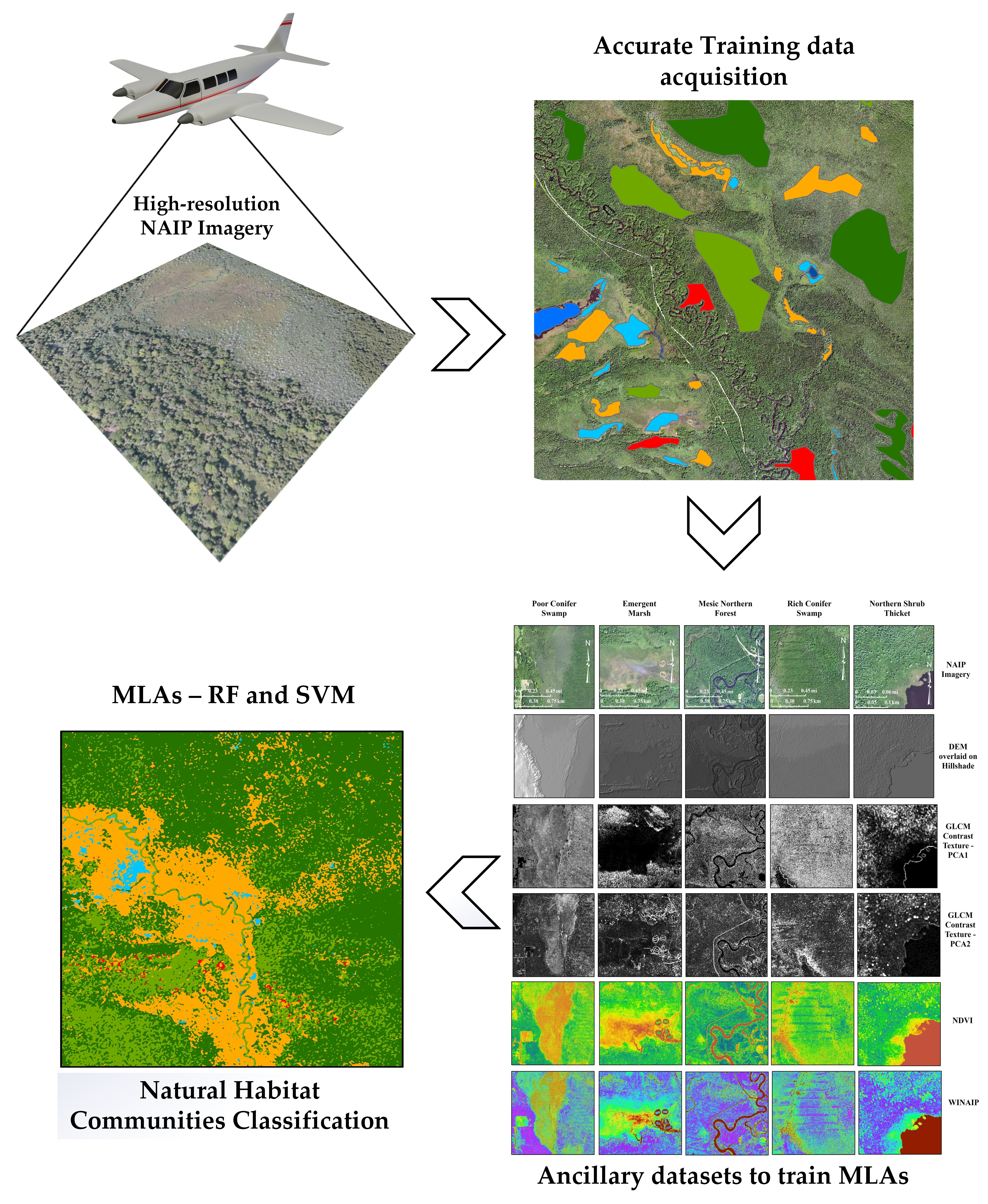
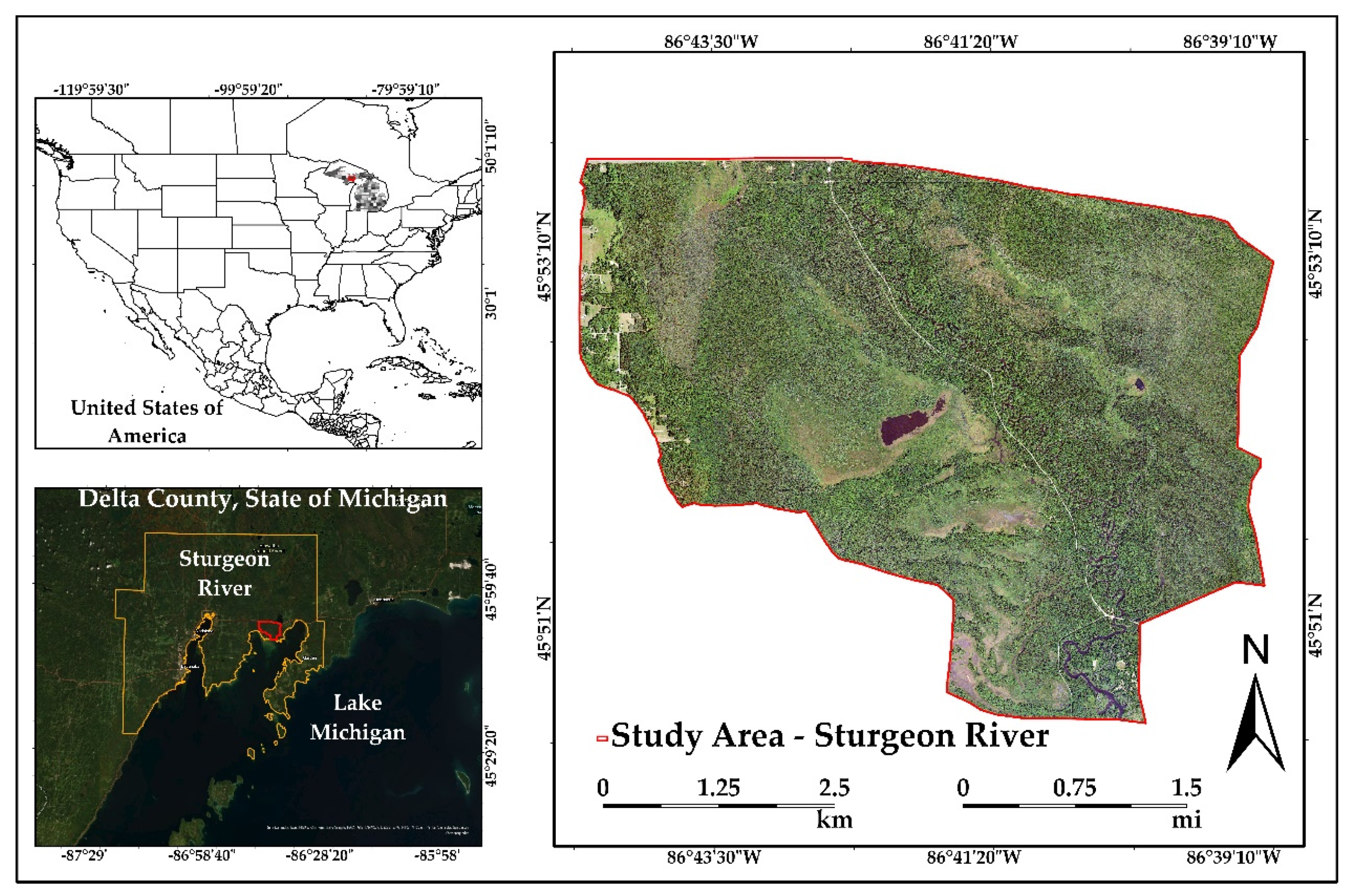
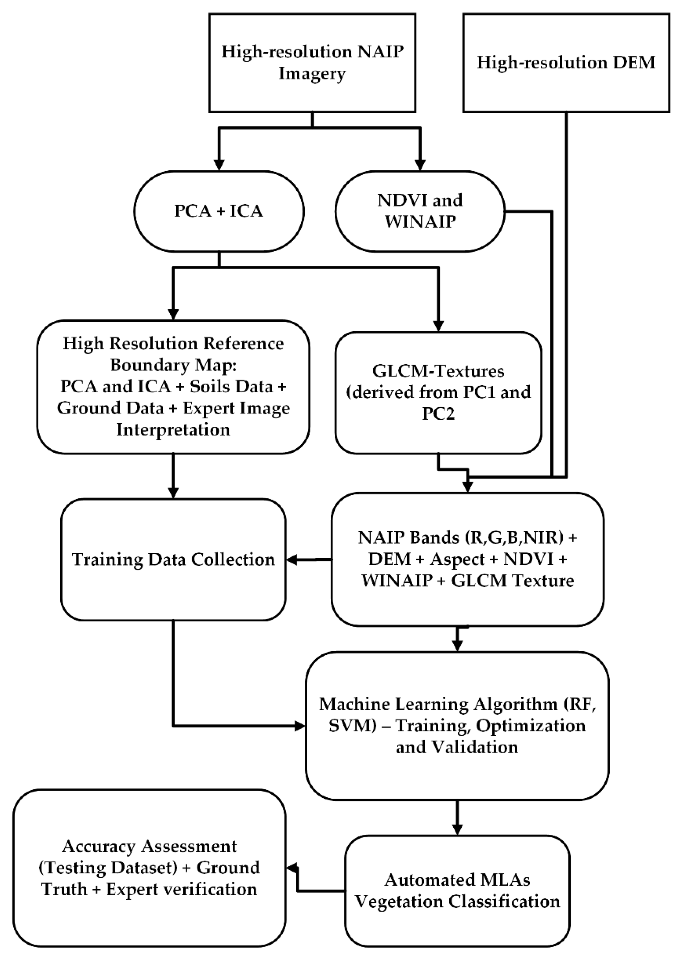
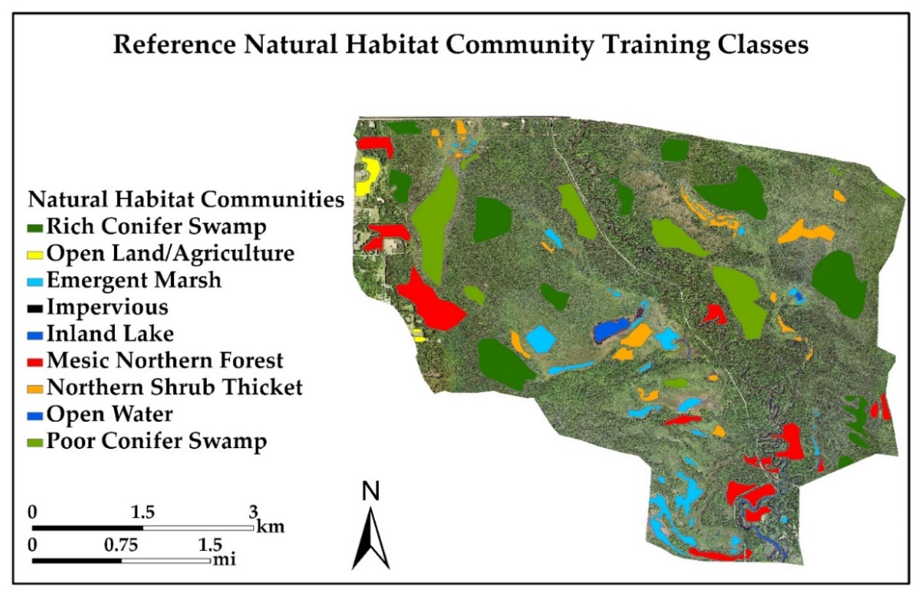
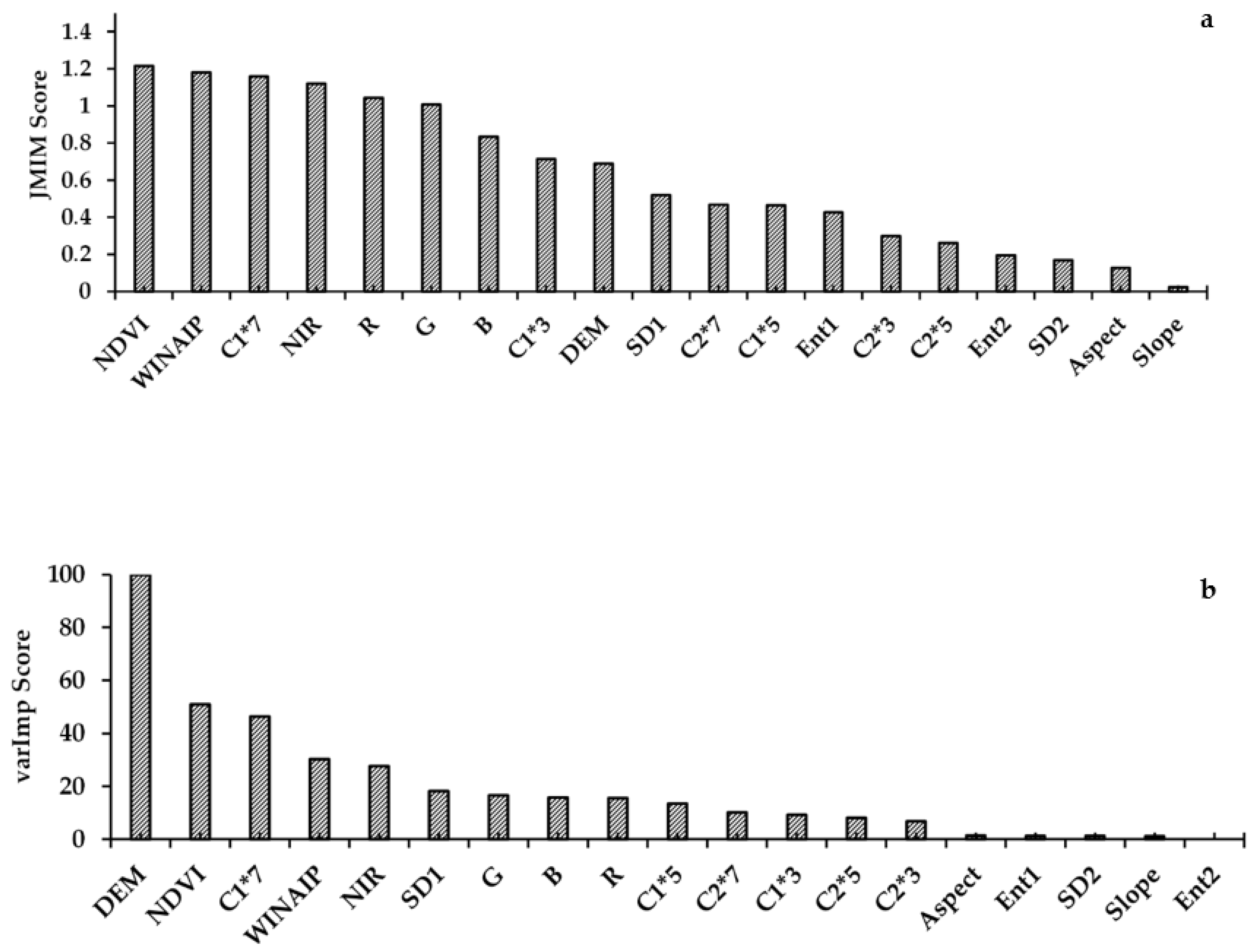
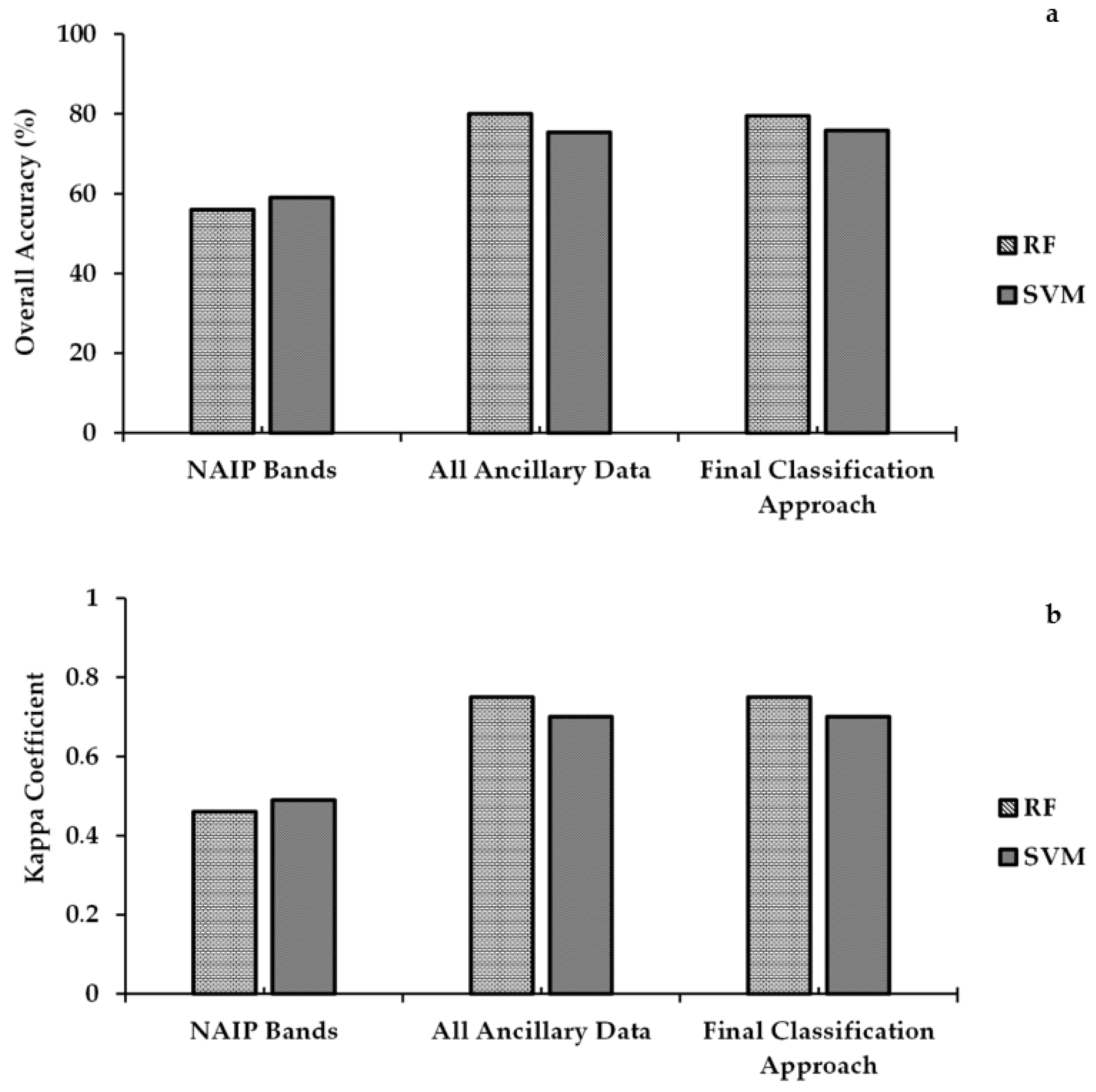
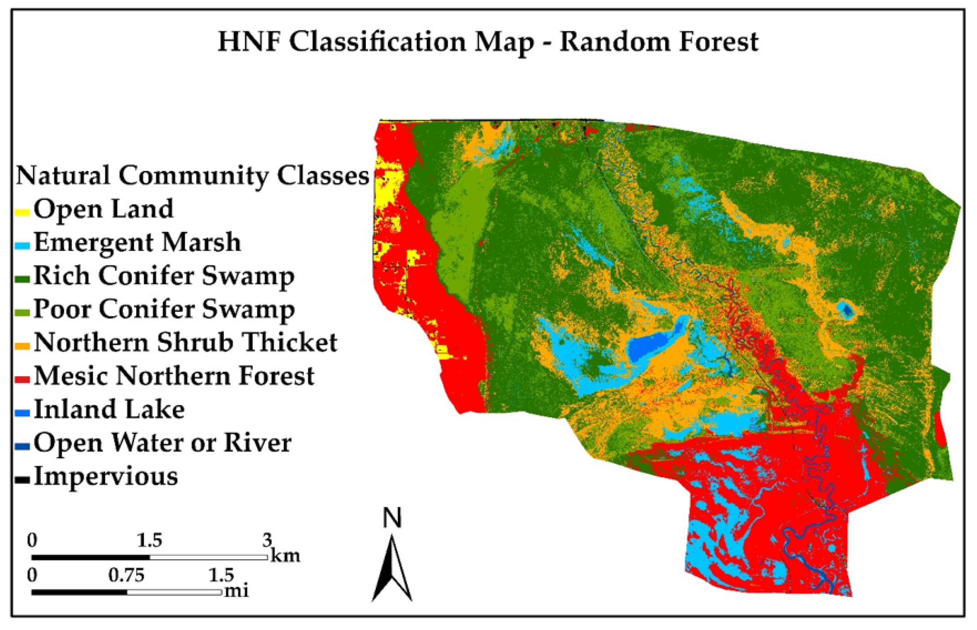
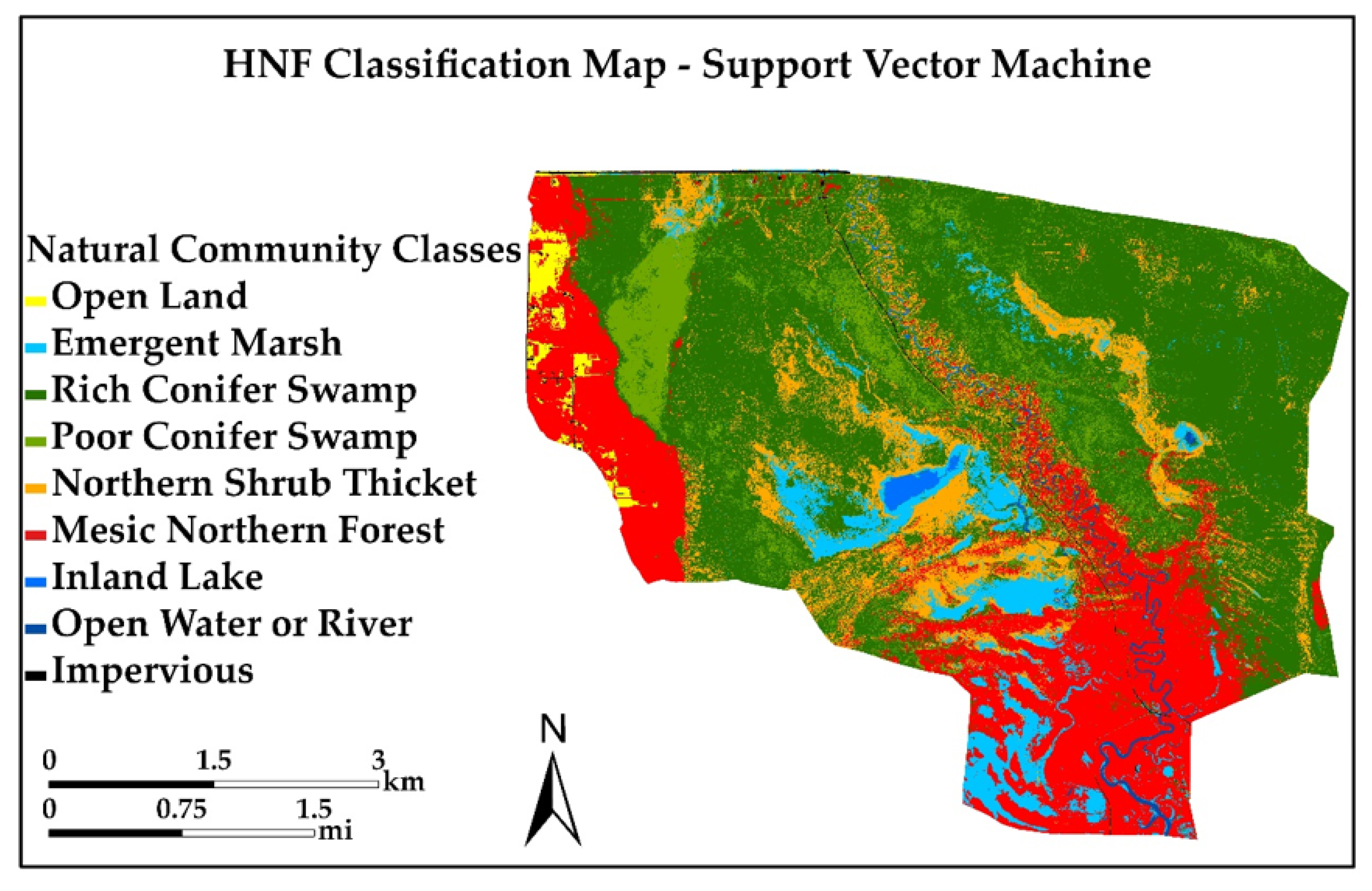
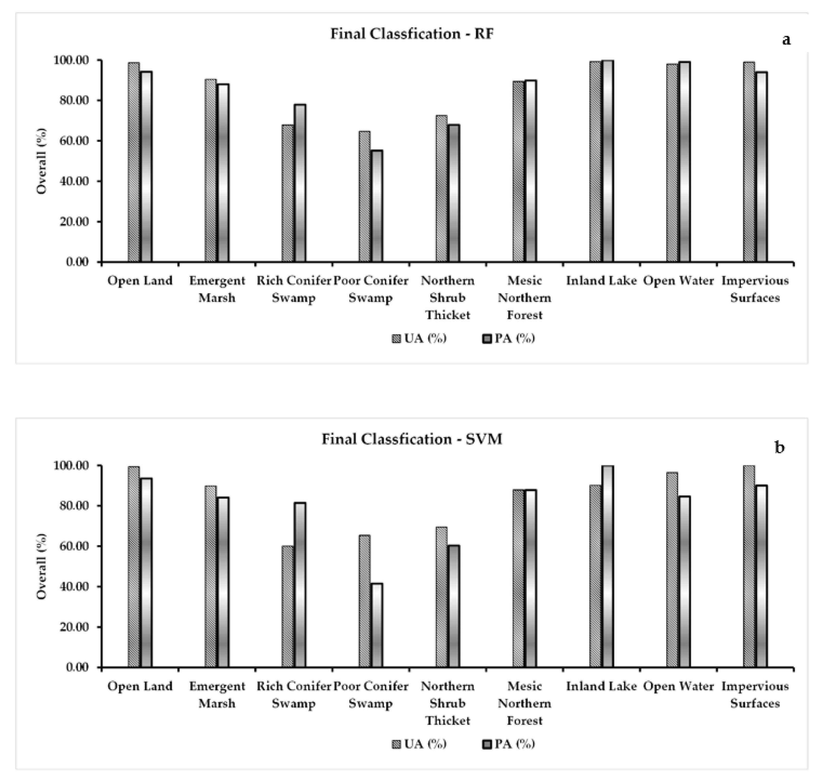
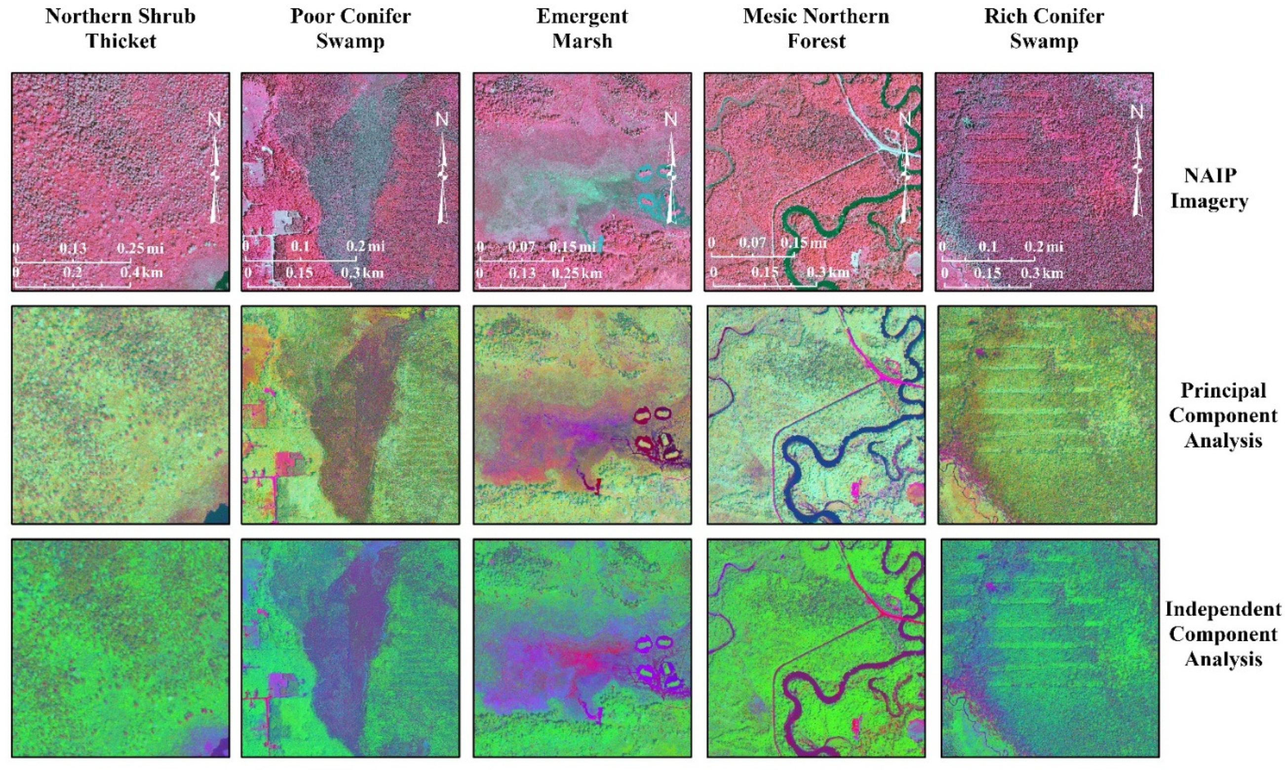
Table 1.
Spectral characteristics of the NAIP data (Leica Geosystems, 2020).
| Spectral Band Names | Wavelength (nm) | Spatial Resolution (cm) |
|---|---|---|
| Blue (B) | 435–495 nm | |
| Green (G) | 525–585 nm | 60 |
| Red (R) | 619–651 nm | |
| Near-Infrared (NIR) | 808–882 nm |
Table 2.
Vegetation communities, areas and the number of randomly generated training and testing points for input into the MLAs.
Table 2.
Vegetation communities, areas and the number of randomly generated training and testing points for input into the MLAs.
| Vegetation Community Type (Code) | Area (Hectares) | Training Data | Testing Data (Accuracy Assessment) |
|---|---|---|---|
| Open Land (OL) | 10.6 | 466 | 155 |
| Emergent Marsh (EM) | 64.7 | 3205 | 1068 |
| Rich Conifer Swamp (RCS) | 202.5 | 4057 | 1352 |
| Poor Conifer Swamp (PCS) | 142.9 | 2272 | 757 |
| Northern Shrub Thicket (NST) | 54.9 | 2620 | 873 |
| Mesic Northern Forest (MNF) | 108.3 | 3814 | 1271 |
| Inland Lake (IL) | 8.3 | 386 | 128 |
| Open Water (OW) | 5.3 | 292 | 97 |
| Impervious Surfaces (IS) | 5.5 | 301 | 100 |
| Total | 603 | 17,413 | 5801 |
Table 3.
Overall accuracy (OA) and kappa coefficient (k) for the input variable combinations. Input 4 (bolded) has the highest OA and k and was used for the final natural communities classification. Abbreviations: Asp—aspect, Slp—slope, Tex—GLCM texture (contrast, entropy, standard deviation 7 × 7), Tex1—contrast (7 × 7), Tex2—contrast (3 × 3), Tex3—contrast (5 × 5).
| Input Data | Variable Combinations | OA (%) (RF) | k (RF) | OA (%) (SVM) | k (SVM) |
|---|---|---|---|---|---|
| 1 | NAIP bands | 56.02 | 0.46 | 59.01 | 0.49 |
| 2 | NAIP bands + DEM | 73.09 | 0.67 | 71.21 | 0.65 |
| 3 | NAIP + DEM + Asp+ Slp + Tex + NDVI + WINAIP + Tex2 + Tex3 | 79.96 | 0.75 | 75.35 | 0.70 |
| 4 | NAIP + DEM + Tex1 + NDVI + WINAIP (JMIM based optimal input variables) | 79.45 | 0.75 | 75.85 | 0.70 |
Table 4.
Kappa values, associated Z-scores and 95% confidence intervals for the input variable combinations. The pairwise Z-score indicates whether the classifications from RF and SVM with the same input variables are statistically different. Abbreviations: Asp—aspect, Slp—slope, Tex—GLCM texture (contrast, entropy, standard deviation 7 × 7), Tex1—contrast (7 × 7), Tex2—contrast (3 × 3), Tex3—contrast (5 × 5).
| Input Number | Variable Combinations | k (RF) | Z-Score (RF) | k (SVM) | Z-Score (SVM) | Z-Score (Pairwise) | 95% CI (RF) | 95% CI (SVM) |
|---|---|---|---|---|---|---|---|---|
| 1 | NAIP bands | 0.46 | 2.37 | 0.49 | 2.72 | −0.34 | ±1.28 | ±1.27 |
| 2 | NAIP bands + DEM | 0.67 | 5.02 | 0.65 | 5.09 | 0.196 | ±1.15 | ±1.17 |
| 3 | NAIP + DEM + Asp + Slp + Tex + NDVI + WINAIP + Tex2+ Tex3 | 0.75 | 6.29 | 0.70 | 6.13 | 0.467 | ±1.02 | ±1.11 |
| 4 | NAIP + DEM + Tex1 + NDVI + WINAIP | 0.75 | 6.29 | 0.70 | 6.13 | 0.467 | ±1.04 | ±1.10 |
Table 5.
Error matrixes and accuracy statistics derived from the final (Input 4) random forest and support vector machine classifications. RF—random forest, SVM—support vector machine, OL—Open Land, EM—Emergent Marsh, RCS—Rich Conifer Swamp, PCS—Poor Conifer Swamp, NST—Northern Shrub Thicket, MNF—Mesic Northern Forest, IL—Inland Lake, OW—Open Water, IS-Impervious, UA—user’s accuracy, PA—producer’s accuracy, OA—overall accuracy, k—kappa.
| RF | OL | EM | RCS | PCS | NST | MNF | IL | OW | IS | Total | UA (%) | PA (%) |
| OL | 146 | 0 | 0 | 0 | 0 | 1 | 0 | 0 | 1 | 148 | 98.64 | 94.19 |
| EM | 0 | 940 | 20 | 8 | 61 | 10 | 0 | 0 | 0 | 1039 | 90.47 | 88.01 |
| RCS | 0 | 42 | 1053 | 275 | 128 | 53 | 0 | 0 | 1 | 1552 | 67.85 | 77.88 |
| PCS | 0 | 10 | 176 | 418 | 23 | 17 | 0 | 1 | 1 | 646 | 64.70 | 55.22 |
| NST | 0 | 59 | 81 | 37 | 592 | 47 | 0 | 0 | 0 | 816 | 72.55 | 67.81 |
| MNF | 9 | 14 | 22 | 19 | 69 | 1142 | 0 | 0 | 3 | 1278 | 89.36 | 89.85 |
| IL | 0 | 1 | 0 | 0 | 0 | 0 | 128 | 0 | 0 | 129 | 99.22 | 100.00 |
| OW | 0 | 2 | 0 | 0 | 0 | 0 | 0 | 96 | 0 | 98 | 97.96 | 98.97 |
| IS | 0 | 0 | 0 | 0 | 0 | 1 | 0 | 0 | 94 | 95 | 98.95 | 94.00 |
| Total | 155 | 1068 | 1352 | 757 | 873 | 1271 | 128 | 97 | 100 | 5801 | OA = 79.45%, k = 0.75 | |
| SVM | OL | EM | RCS | PCS | NST | MNF | IL | OW | IS | Total | UA (%) | PA (%) |
| OL | 145 | 0 | 0 | 0 | 0 | 1 | 0 | 0 | 0 | 146 | 99.31 | 93.55 |
| EM | 0 | 898 | 21 | 6 | 66 | 7 | 0 | 0 | 1 | 999 | 89.88 | 84.08 |
| RCS | 0 | 71 | 1101 | 371 | 196 | 93 | 0 | 0 | 0 | 1832 | 60.09 | 81.43 |
| PCS | 0 | 3 | 139 | 314 | 11 | 11 | 0 | 1 | 1 | 480 | 65.41 | 41.48 |
| NST | 0 | 81 | 72 | 35 | 526 | 43 | 0 | 0 | 0 | 757 | 69.48 | 60.25 |
| MNF | 10 | 12 | 19 | 31 | 74 | 1116 | 0 | 0 | 8 | 1270 | 87.87 | 87.80 |
| IL | 0 | 0 | 0 | 0 | 0 | 0 | 128 | 14 | 0 | 142 | 90.14 | 100.00 |
| OW | 0 | 3 | 0 | 0 | 0 | 0 | 0 | 82 | 0 | 85 | 96.47 | 84.53 |
| IS | 0 | 0 | 0 | 0 | 0 | 0 | 0 | 0 | 90 | 90 | 100.00 | 90.00 |
| Total | 155 | 1068 | 1352 | 757 | 873 | 1271 | 128 | 97 | 100 | 5801 | OA = 75.85%, k = 0.70 | |
Publisher’s Note: MDPI stays neutral with regard to jurisdictional claims in published maps and institutional affiliations. |
© 2022 by the authors. Licensee MDPI, Basel, Switzerland. This article is an open access article distributed under the terms and conditions of the Creative Commons Attribution (CC BY) license (https://creativecommons.org/licenses/by/4.0/).
Share and Cite
MDPI and ACS Style
Bhatt, P.; Maclean, A.; Dickinson, Y.; Kumar, C. Fine-Scale Mapping of Natural Ecological Communities Using Machine Learning Approaches. Remote Sens. 2022, 14, 563. https://doi.org/10.3390/rs14030563
AMA Style
Bhatt P, Maclean A, Dickinson Y, Kumar C. Fine-Scale Mapping of Natural Ecological Communities Using Machine Learning Approaches. Remote Sensing. 2022; 14(3):563. https://doi.org/10.3390/rs14030563
Chicago/Turabian StyleBhatt, Parth, Ann Maclean, Yvette Dickinson, and Chandan Kumar. 2022. "Fine-Scale Mapping of Natural Ecological Communities Using Machine Learning Approaches" Remote Sensing 14, no. 3: 563. https://doi.org/10.3390/rs14030563
Note that from the first issue of 2016, this journal uses article numbers instead of page numbers. See further details here.