Article

An Observing System Simulation Experiment Framework for Air Quality Forecasts in Northeast Asia: A Case Study Utilizing Virtual Geostationary Environment Monitoring Spectrometer and Surface Monitored Aerosol Data

1
Department of Urban and Environmental Engineering, Ulsan National Institute of Science and Technology, Ulsan 44919, Korea
2
Global Environment Research Division, National Institute of Environmental Research, Incheon 22689, Korea
*
Author to whom correspondence should be addressed.
Remote Sens. 2022, 14(2), 389; https://doi.org/10.3390/rs14020389
Submission received: 16 November 2021 / Revised: 5 January 2022 / Accepted: 12 January 2022 / Published: 14 January 2022

Abstract

:
Prior knowledge of the effectiveness of new observation instruments or new data streams for air quality can contribute significantly to shaping the policy and budget planning related to those instruments and data. In view of this, one of the main purposes of the development and application of the Observing System Simulation Experiments (OSSE) is to assess the potential impact of new observations on the quality of the current monitoring or forecasting systems, thereby making this framework valuable. This study introduces the overall OSSE framework established to support air quality forecasting and the details of its individual components. Furthermore, it shows case study results from Northeast Asia and the potential benefits of the new observation data scenarios on the PM2.5 forecasting skills, including the PM data from 200 virtual monitoring sites in the Gobi Desert and North Korean non-forest areas (NEWPM) and the aerosol optical depths (AOD) data from South Korea’s Geostationary Environment Monitoring Spectrometer (GEMS AOD). Performance statistics suggest that the concurrent assimilation of the NEWPM and the PM data from current monitoring sites in China and South Korea can improve the PM2.5 concentration forecasts in South Korea by 66.4% on average for October 2017 and 95.1% on average for February 2018. Assimilating the GEMS AOD improved the performance of the PM2.5 forecasts in South Korea for October 2017 by approximately 68.4% (~78.9% for February 2018). This OSSE framework is expected to be continuously implemented to verify its utilization potential for various air quality observation systems and data scenarios. Hopefully, this kind of application result will aid environmental researchers and decision-makers in performing additional in-depth studies for the improvement of PM air quality forecasts.

1. Introduction

Air quality deterioration owing to the abundance of PM2.5 (particulate matter with an aerodynamic diameter below 2.5 μm) is a widespread and severe environmental problem threatening human and ecosystem health [1]. Air quality prediction or the forecasting of PM2.5 air quality is a useful tool for the governmental agencies in terms of planning and for the public with regard to health protection and air quality management. However, there are significant differences between the predicted and observed concentrations, due to the high uncertainties embedded in the numerical simulation of atmospheric PM. Therefore, enhancing the accuracy of PM2.5 concentration prediction by adding more and reliable information to the modelling system is important. Data assimilation (DA), where the observation information is combined with the atmospheric models, can help improve PM simulation by reducing the uncertainties in the input data, such as the initial conditions or boundary conditions. This means that a sufficient volume of observation data that adequately reflects the spatial and temporal features of aerosol pollution is necessary for the DA to function properly [2].
The regular surface monitoring of the air quality in the aforementioned areas would provide routine and basic information for the more optimized predictions and management of regional air quality. In addition to surface observations, satellite observations can improve the accuracy of PM air quality forecasts by providing spatially extensively scanned air pollution data in real or semi-real time, including in locations that surface monitoring cannot cover. Until now, aerosol properties have been observed widely by a number of low earth orbit (LEO) satellites [3]. The Korean Geostationary Environment Monitoring Spectrometer (GEMS) was launched on 18 February 2020, equipped with an UV-VIS spectrometer that enables fast sampling at higher temporal resolutions than the LEO satellites. The GEMS can scan the air quality in East Asia up to eight times during the daytime and can continuously observe air pollutants over the Asian region [3]. Although complete datasets have not yet been publicly disclosed by the Environmental Satellite Centre (ESC, https://nesc.nier.go.kr/, accessed on 8 July 2021), it is necessary to develop a routine approach in advancing toward the use of these data with regard to improving air quality forecasting, in case they become available.
A tremendous amount of human and financial resources is required to develop an integrated observation framework, including surface observation networks and space-borne satellites. Therefore, a prior evaluation of the potential benefits of using new observational instruments would be very helpful. In this sense, the OSSE can objectively justify the additional value from and optimal design of new observation systems [4]. OSSEs refer to a set of experiments that estimate the potential impact of future observing systems in an existing monitoring or forecasting system [4]. The OSSE has been widely applied in the meteorological research fields [5], but its use in the field of air quality management, particularly with regard to aerosols, has been limited [4].
The air quality over the Korean Peninsula varies significantly depending on the regional emission distributions and meteorological patterns. The air quality of South Korea, located downwind of large anthropogenic emissions and natural dust sources in North Korea and China, is highly likely to be affected by transboundary particulate air pollution. For example, biomass fuel-burning activities in North Korea may significantly degrade the air quality in Seoul, South Korea [6]. Moreover, Asian dust transported from the Gobi Desert and other deserts over the southern part of Mongolia can affect the air quality of downwind regions, including eastern China and the Korean peninsula [7,8].
We established an OSSE framework to improve the forecasting of PM2.5 air quality on the Korean Peninsula and in the surrounding areas in Northeast Asia. In this paper, we first describe the sub-modules and key technical elements of the OSSE framework that we developed. Then, we present the results of an application of the OSSE framework that assesses the potential impacts of the expanded surface observation network and the utilization of aerosol optical depth (AOD) observations from a virtual GEMS on the PM2.5 air quality forecasting in Northeast Asia for October 2017 and February 2018, respectively.

2. Materials and Methods

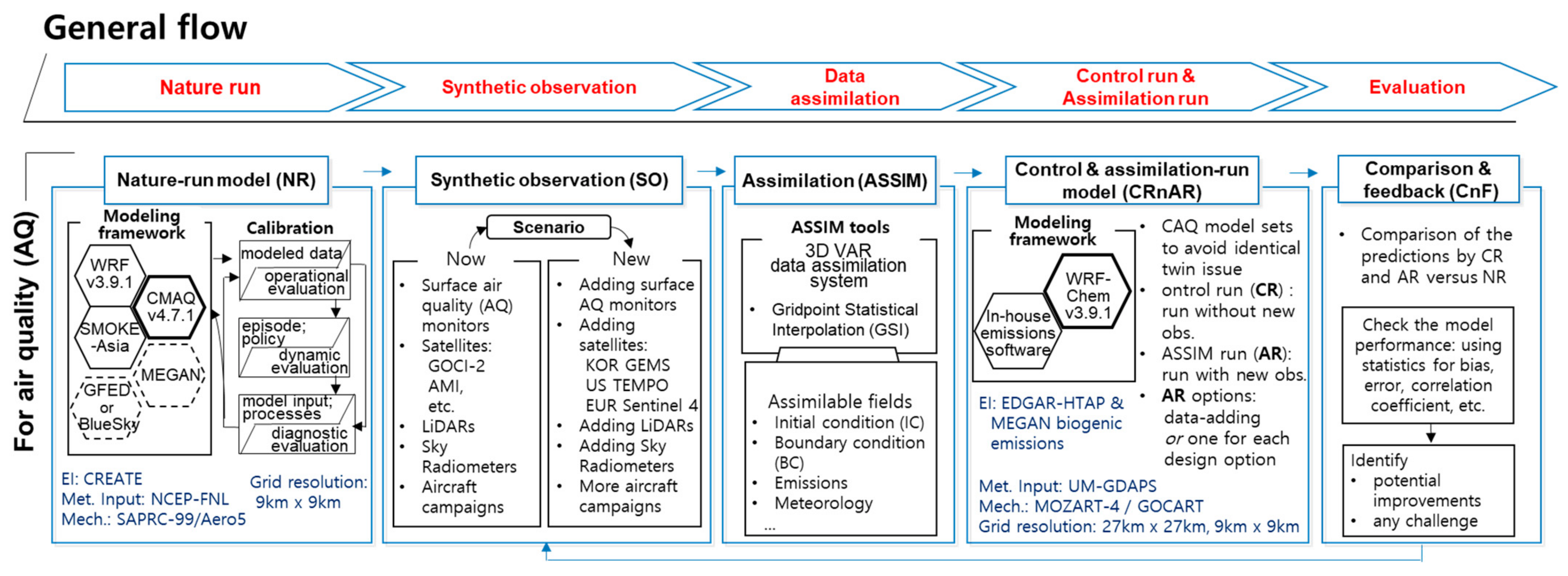
2.1. OSSE Framework for Regional Air Quality Forecasting

The OSSE has a variety of practical applications and the organization of the OSSE framework depends heavily on its intended use. The OSSE framework developed here consists of five sub-modules: nature run (NR); synthetic observation (SO); data assimilation (ASSIM); control run and assimilation run (CRnAR); and comparison and feedback (CnF) (Figure 1).

2.1.1. Nature Run Module

NR is the module where a simulation is performed to generate a reference that is close to the observed atmospheric state. This module uses a three-dimensional Eulerian chemistry transport model with a good performance and at the highest available spatial resolution. As shown in Figure 1, for the simulation of the most natural air quality state, the Community Multiscale Air Quality (CMAQ) model version 4.7.1 [9,10] was employed. This CMAQ model is being used as one of the main models at the Air Quality Forecast Center of Korea (e.g., [11,12]). The meteorological fields were specified from the simulations by the Weather Research and Forecasting Model (WRF) version 3.9.1. The emissions input into the CMAQ model were from the SMOKE-Asia version 1.3.1 [13]. The emission inventory for air pollutants used in the NR module was the Comprehensive Regional Emissions inventory for Atmospheric Transport Experiments version 2015 (CREATE 2015) [14]. The CREATE 2015 is an updated version of the air pollutant emissions of the year 2010 from the anthropogenic source in East Asia [14]. If necessary, a biogenic emission (e.g., MEGAN [15]) and a biomass burning emission (e.g., BlueSky [16] or Global Fire Emissions Database (GFED) [17]) model or database could be included in the NR module.
The NR modelling system was established at a high-resolution system (9 km × 9 km) in East Asia (Figure 2). The NR is not perfect, and its drawbacks should be investigated against the actual observational data; if the drawbacks could hinder the purpose of the OSSE, then the NR may need to be calibrated [5,18].

2.1.2. Synthetic Observation Module

The SO module allows for synthetic observation corresponding to a potential observation system or device. For the SO, the methodology that reconstructs the data of the potential measurement device considered in the scenario should be established. SO is created by reflecting the specifications of the potential observation equipment in the NR results, such as observation strategy, data retrieval algorithm, and observation error characteristics. In this module, the SO production is conducted in three steps: (1) scenario determination for the measuring equipment; (2) data creation and inputting for the SO calculation; and (3) SO calculation and preparing appropriate dimensional data for the scenario. Specific details on the data reconstruction are presented in the “Scenarios and data reconstruction” section.

2.1.3. Assimilation Module

In this module, the synthetic observation (SO) sets for PM2.5, PM10, and AOD from the virtual systems are provided for another model to perform DA in the spacetime dimension of the model. We used the WRF model coupled with chemistry (WRF–Chem) version 3.9.1, implemented with the Goddard Chemistry Aerosol Radiation and Transport (GOCART) [19] aerosol scheme. The data assimilation technique was based on the three-dimensional variational (3-D VAR) method coded by the National Centres for Environmental Prediction (NCEP) Gridpoint Statistical Interpolation (GSI) [20,21,22]. The GSI 3D-VAR was used to determine the optimal analysis field that minimizes the cost function J, which is expressed as follows:
2 J x = x x b T B 1 x x b + y 0 H x T R 1 y 0 H x ,
where x is a vector of analysis; x b   is the forecast or background vector; y 0 is an observation vector;   B is the background error covariance (BEC) matrix; H is an observation operator; and R is the observation error covariance matrix.
For the DA of any observation with the GSI system, a model-simulated observation is required at the locations of the observation through the observation operator (or “forward operator”). Model simulated PM2.5, PM10, and AOD were reconstructed by aggregating individual aerosol species simulated from the WRF–Chem GOCART module.
PM2.5 and PM10 are calculated as follows:
PM 2.5 =   ρ P 2.5 + 1.375 Sulfate + B C 1 + B C 2 + 1.8 O C 1 + O C 2 + D 1 + 0.286 D 2 + S S 1 + 0.942 S S 2 ,
PM 10 =   ρ P 2.5 + 1.375 Sulfate + B C 1 + B C 2 + 1.8 O C 1 + O C 2 + D 1 + D 2 + D 3 + 0.87 D 4 + S S 1 + S S 2 + S S 3 ,
where ρ is dry air density; P 2.5 represents the unspecified fine aerosols; Sulfate denotes sulfate aerosols; D 1 , D 2 , and D 3 ( S S 1 , S S 2 , and S S 3 ) denote mineral dust (sea salt) aerosols in the three smallest particle size bins and D4 is mineral dust in the fourth smallest particle size bin (effective radius of 4.5 mm); and O C 1 and O C 2 ( B C 1 and B C 2 ) are hydrophobic and hydrophilic OC (BC), respectively.
The AOD ( τ ) for each aerosol type is expressed as follows:
τ λ = i = 1 n k = 1 k top E e x t λ , n r i , r e f f i   c i k   ρ d k   d k ,
where E e x t denotes the extinction coefficient; c i k represents the aerosol mass for species i at the kth layer; ρd is dry air density; and d denotes layer depth. Here, Eext is defined as a function of wavelength λ, refractive index n r i , and effective radius r e f f i .
Additional details on the observation operators for PM2.5, PM10, and AOD are reported by [23,24,25].
The background error covariance matrix B   was computed using the National Meteorological Center (NMC) method [26] that calculates systematic errors according to the model simulation time difference. In this study, the 24-h and 12-h forecasting datasets were used to derive the model background error covariance for each month. In this manner, the statistical data of error were generated for 15 aerosols (sulfate, carbon component, sand dust, sea salt, and the remaining ultrafine dust) in the GOCART scheme [19].
For the observation error covariance regarding the PM2.5 and PM10 data synthesized from the NR, the error formula used in the observing system experiment (OSE) was applied. Measurement ( ε M ) and representative ( ε R ) errors were specified for each PM observation value ( P o b s ) with preset parameters as in the following formulas [25,27]:
ε M = 1.5 + 0.0075   P o b s ,
ε R = ε T   ε M   Δ x L ,
where ε T is the adjustable parameter set as 0.5, as reported by Schwartz et al. [28];   Δ x is the model grid resolution (27 km for domain 1 and 9 km for domain 2 in this case); and ε L U is the radius of the influence of an observation, specified as 3 km here according to Elbern et al. [27]. Then the total PM error ( ε P M ) is represented as:
ε P M = ε M 2 + ε R 2 .
The total observation errors for the virtual GEMS AOD ( ε A O D ) are defined differently depending on whether the AOD is observed over the ocean or on land:
ε o c e a n = 0.185 τ + 0.037 ,
ε l a n d = 0.137 τ + 0.08 ,
where, ε w a t e r and ε L a n d are the observation errors at sea and on land, respectively [29]. Additional details on the assimilation system are available in Kim et al. [30].
It is noted that the criteria for thinning performed before applying the GEMS AOD value to the GSI data assimilation system were adjusted, which improved the quality of data assimilation significantly. After the sensitivity tests, the thinning interval for the GEMS satellite AOD data assimilation was empirically set to 27 km for domain 1 and 9 km for domain 2, in accordance with the horizontal resolution of the model.

2.1.4. Control Run and Assimilation Run Module

In this module, two types of models are established and are usually performed in parallel. The first is the control run (CR) that is performed without employing any DA. The second is the assimilation run (AR), where the synthesized data for the new instrument (i.e., SO) are assimilated. It is important to use different models for the NR and the control and assimilation runs (CR and AR) to avoid the identical or fraternal twin problem and to obtain more realistic results from the full OSSE [5,18]. The identical twin problem means that the forecast attains excessively optimistic results due to the use of the same model for both nature and assimilation runs. Instead of using the model setting used for NR (i.e., CMAQ model), this CRnAR module uses the Weather Research and Forecasting model coupled with Chemistry (WRF–Chem) model version 3.9.1 [31].
The CR and AR using WRF–Chem were performed in the two domains simultaneously. The first modelling domain (Domain 01, D01) covered the Northeast Asia region at a horizontal resolution of 27 km, and the second (D02) was nested within Domain 1, focusing on the Korean Peninsula with a 9 km × 9 km horizontal grid system. The model grid system contained 31 vertical levels topped at 50 hPa. In order to further avoid the identical twin problem and to induce more differences between the model results, we used the Emission Database for Global Atmospheric Research–Hemispheric Transport of Air Pollution (EDGAR–HTAP) [32,33] as the anthropogenic emission input. We also used biogenic emissions and dust emissions that were calculated online using the Model of Emissions of Gases and Aerosols from Nature (MEGAN) [15] and the GOCART module, respectively (Table 1). The employed physical parameterizations in the WRF–Chem model include the Grell-3D scheme for cumulus convection, the Single Moment-6 (WSM6) for cloud microphysics, the Unified Noah Land Surface Model for the land surface, the Yonsei University (YSU) scheme for the planetary boundary layer (PBL), the Goddard shortwave scheme, and the Rapid Radiative Transfer Model (RRTM) for longwave. Refer to [30] and the references therein.

2.1.5. Comparison and Feedback Module

In this module, by comparing the errors of the CR and AR results to those from the NR, the value of the data scenarios that can be brought to the key research objective (e.g., the improvement of the fine PM forecasting score) was evaluated. Three statistics were used to compare the model performance: mean bias (MB); root mean square error (RMSE); and correlation coefficient (r). Furthermore, a percentage of improvement (PI) [35] for the AR was calculated to quantify the efficiency of the model running with DA (i.e., AR).
The MB is expressed as follows:
Mean   Bias   MB = 1 N 1 N M i O i ,
where M i denotes the modeled concentration; O i is the observed concentration; and N is the number of data samples. The closer the MB is to 0, the more optimized the prediction performance.
The RMSE is determined as follows:
RMSE = 1 N M i O i 2 N .
When the RMSE is close to 0, the model performs better in the prediction.
The r is expressed as follows:
r = 1 n 1 1 N O i O ¯ σ O · M i M ¯ σ M ,
where O ¯ , M ¯ , σ O , and σ M represent the mean and the standard deviation of the observations and model forecasts, respectively. The value of r ranges between −1 and 1, with the strongest negative linear relationship at r = −1 and the strongest positive linear relationship at r = 1.
The percentage of improvement (PI) is expressed as follows:
P I A R = 100 1 R M S E A R R M S E C R 2 ,
where R M S E A R and R M S E C R are the RMSE values of AR and CR, respectively. The closer the PI is to 100%, the more optimized the method improvement.

2.2. Implementation of PM2.5 Forecasting

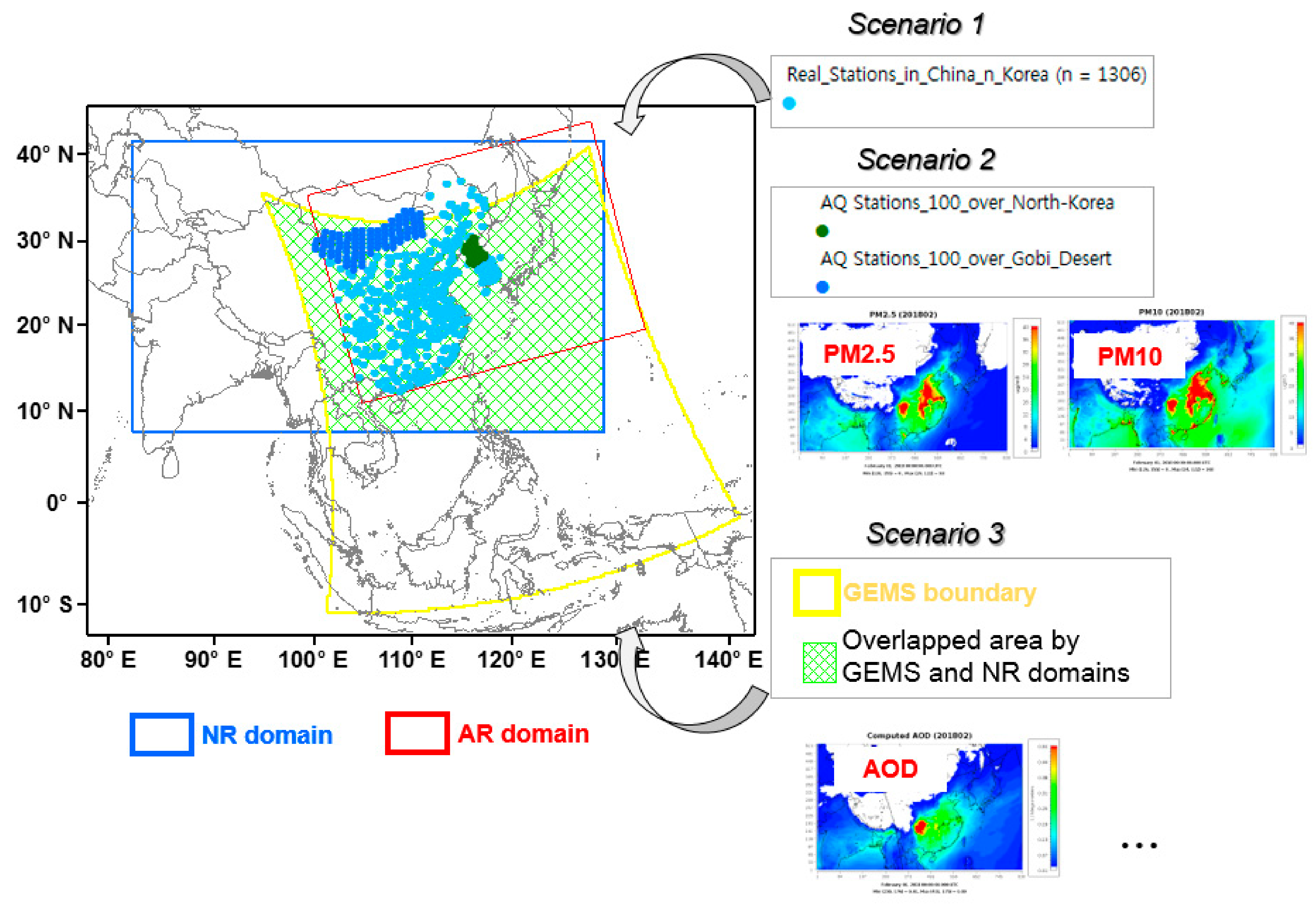
2.2.1. Spatial and Temporal Scope

This study conducted a case study to highlight the purpose of applying the OSSE framework described in the Methods section, for which we developed a testbed modelling system at a high horizontal resolution (9 km × 9 km) using CMAQ (Figure 2 and Table 1), and examined whether it performed stably. The spatial domain of the OSSE testbed was in East Asia. Specifically, the NR domain ranged within a latitude of 10 to 58° and longitude of 51 to 160° (shown in blue in Figure 2). However, the CR and AR were conducted in domains (shown in red in Figure 2) smaller than the NR. By applying the new data scenarios to the testbed, we examined the improvement of the PM2.5 forecasting skills for October 2017 and February 2018. It should be noted that the base year of the emission inventory (EI) that we used focused on the emissions of air pollutants in 2015, not 2017 or 2018. The EI for the year 2015 was the best available when we were conducting this study.

2.2.2. Scenarios and Data Reconstruction

Using the NR results, we reconstructed the sets of synthetic observation (SO) data for the new observation data scenarios in China and Korea. The first scenario was sustaining the current surface monitoring networks in China and South Korea without any changes (Scenario 1 in Figure 3). Using the NR results, the concentration fields of PM2.5 and PM10 were reconstructed as follows:
PM 2.5 = F i n e   S u l f a t e + F i n e   N i t r a t e + F i n e   A m m o n i u m + E l e m e n t a l   C a r b o n + F i n e   O r g a n i c   M a t t e r + F i n e   S e a   S a l t + U n s p e c i a t e d   F i n e   P a r t i c l e ,
PM 10 = PM 2.5 + C o a r s e   P a r t i c l e ,
where coarse particles include the coarse mode particulates of sea salt, sulfate, ammonium, nitrate, and the inert crustal species (i.e., ASOIL and ACORS in the CMAQv4.7.1 model).
Then, the reconstructed PM2.5 and PM10 concentration fields at the surface monitoring sites (1306 sites) located in China and South Korea were extracted and converted into the SO database for the application of the data assimilation (i.e., AR1 in Table 1).
The second scenario entailed installing 100 PM observatories each in North Korea and in the Gobi Desert, and a simulation was performed to evaluate whether this observing plan would be helpful for PM2.5 forecasting (Scenario 2 in Figure 3). In scenario 2, the reconstructed PM2.5 and PM10 concentration fields were also extracted at the locations of the added surface air monitoring sites in North Korea and the Gobi Desert in the NR simulation data. Then, SO datasets for PM2.5 and PM10 were derived at 200 virtual measurement points in North Korea and the Gobi Desert and used for the data assimilation (AR2 in Table 1).
The third scenario entailed utilizing the AOD data from the Korea geostationary orbiting satellites (GEMS) (Scenario 3 in Figure 3) for the data assimilation in the OSSE to improve the prediction accuracy of PM2.5 in the domain. The AOD values were calculated based on the NR results from the area where the GEMS scanning range (yellow-lined area in Figure 3) overlapped with the NR (blue-lined area in Figure 4) and AR model domain areas (red-lined area in Figure 3). The AOD values located in the overlapped areas between the NR and AR model domains (green area in Figure 3) were extracted and used for data assimilation (AR3 in Table 1).
The SO database construction for AOD was more complicated than that for the PM. The virtual AOD was reconstructed by integrating the aerosol extinction coefficient ( B e x t ) with regard to the vertical height (z) of the NR model:
AOD = B e x t z   d z .
B e x t values were calculated from the mass concentration of the major aerosol components by applying the revised version of the Interagency Monitoring of Protected Visual Environments (IMPROVE) algorithm [33] to the chemical and meteorological variables calculated from the NR:
B e x t = 2.2   f S R H   S m a l l   S u l f a t e + 4.8   f L R H   L a r g e   S u l f a t e + 2.4   f S R H   S m a l l   N i t r a t e + 5.1   f L R H   L a r g e   N i t r a t e + 2.8   S m a l l   O r g a n i c   M a s s + 6.1   L a r g e   O r g a n i c   M a s s + 10   E l e m e n t a l   C a r b o n + F i n e   S o i l + 1.7   f S S R H   S e a   S a l t + 0.6   C o a r s e   P a r t i c l e .
Details on splitting the aerosol species (i.e., sulfate, nitrate, and total organic mass) into small and large size groups and allocating hygroscopic growth factors for the different size groups of particles can be found in other studies (e.g., [35]).
The CMAQ AOD data computed in this way were stored as potential GEMS AOD data by selecting the data fields located within the determined scan area of the GEMS and then regridding them into each unit grid of the GEMS. In this study, the virtual GEMS AOD data were derived from the following equation:
AOD G E M S = ω × A O D C M A Q ω ,
where ω = A o v e r l a p p e d A G E M S and A o v e r l a p p e d is the individual CMAQ grid area overlapping the grid area of the GEMS ( A G E M S ); and A O D C M A Q denotes the AOD reconstructed using the NR results. The reconstructed GEMS AOD data had a time resolution of 1 h from 00 to 07 UTC at a horizontal resolution of approximately 7 km × 8 km.

3. Results

3.1. Performance of the Nature Run

The proper evaluation of the NR in terms of its spatio-temporal variability and the prevention of the identical twin problem are recommended for the improvement of the OSSE framework and the achievement of more realistic results [5,18,36]. This section shows the evaluation results for the NR simulation performance. We evaluated the CMAQ air quality model of the NR module by comparing the modelled and the observed PM2.5 concentrations at the surface monitoring networks located in China and Korea for October 2017 and February 2018 (Figure 4).
While the NR generally captures the temporal variability of the observed PM2.5 mass concentrations in the domain (correlation coefficient in Figure 4), it tends to underpredict across the domain for both October 2017 and February 2018 (mean bias in Figure 4). The temporal correlation coefficient in the NR tends to decrease further from the neighboring areas of the major metropolitan areas in China and South Korea (e.g., Beijing–Tianjin–Hebei region (BTH), Shandong Peninsula (SDP), Shanghai (SH), Seoul Metropolitan Area (SMA)) to the direction of remote areas (i.e., Inner Mongolia (INM)) in northern China. For instance, the correlation coefficients (r) in October 2017 in BTH, SDP, SH, and SMA were as high as 0.7 (range 0.2–0.9), 0.7 (0.1–0.9), 0.6 (0.4–0.8), and 0.6 (0.3–0.8), respectively, and those in February 2018 were 0.6 (0.1–0.9), 0.6 (0.3–0.9), 0.6 (0.5–0.8), and 0.8 (0.6–0.9), respectively. The estimated correlation coefficients (r) in Inner Mongolia were 0.6 (0.2–0.9) in October 2017 and 0.2 (−0.2–0.7) in February 2018. With regard to bias statistics, the NR also shows better performance in the neighboring areas of the major metropolitan areas than the remote arid land areas in northern China (i.e., INM). The average concentrations of the observed PM2.5 in BTH, SDP, SH, SMA, and INM for October 2017 were 61, 46, 24, 17, and 38 µg/m3, respectively, and those for February 2018 were 69, 59, 44, 32, and 34 µg/m3, respectively. For the observations provided, the NR results in October 2017 in BTH, SDP, SH, SMA, and INM were approximately 35, 40, 40, 56, and 62% lower than the observed values, respectively, and those in February 2018 were approximately 45, 41, 30, 50, and 63% lower, respectively. A previous study [37] proposed the model performance goals (e.g., bias ≤ ± 30%) and criteria (e.g., bias ≤ ± 60%) for fine particulate matter, and these have been actively cited in numerous modelling studies. The NR biases shown over the major metropolitan areas in China and South Korea generally meet the criteria but exceed the goals.
Although the bias only meets the performance criteria, the NR results are being used for subsequent experiments because the current focus is on checking whether the entire system functions correctly. In other words, the NR results are being used as the base data to derive the synthetic observation data (see the next section). Future efforts should be made to improve the predictions in the underpredicted areas in order to achieve more realistic experiment results [5,18]. We discuss the model bias issue in the “NR module” section.

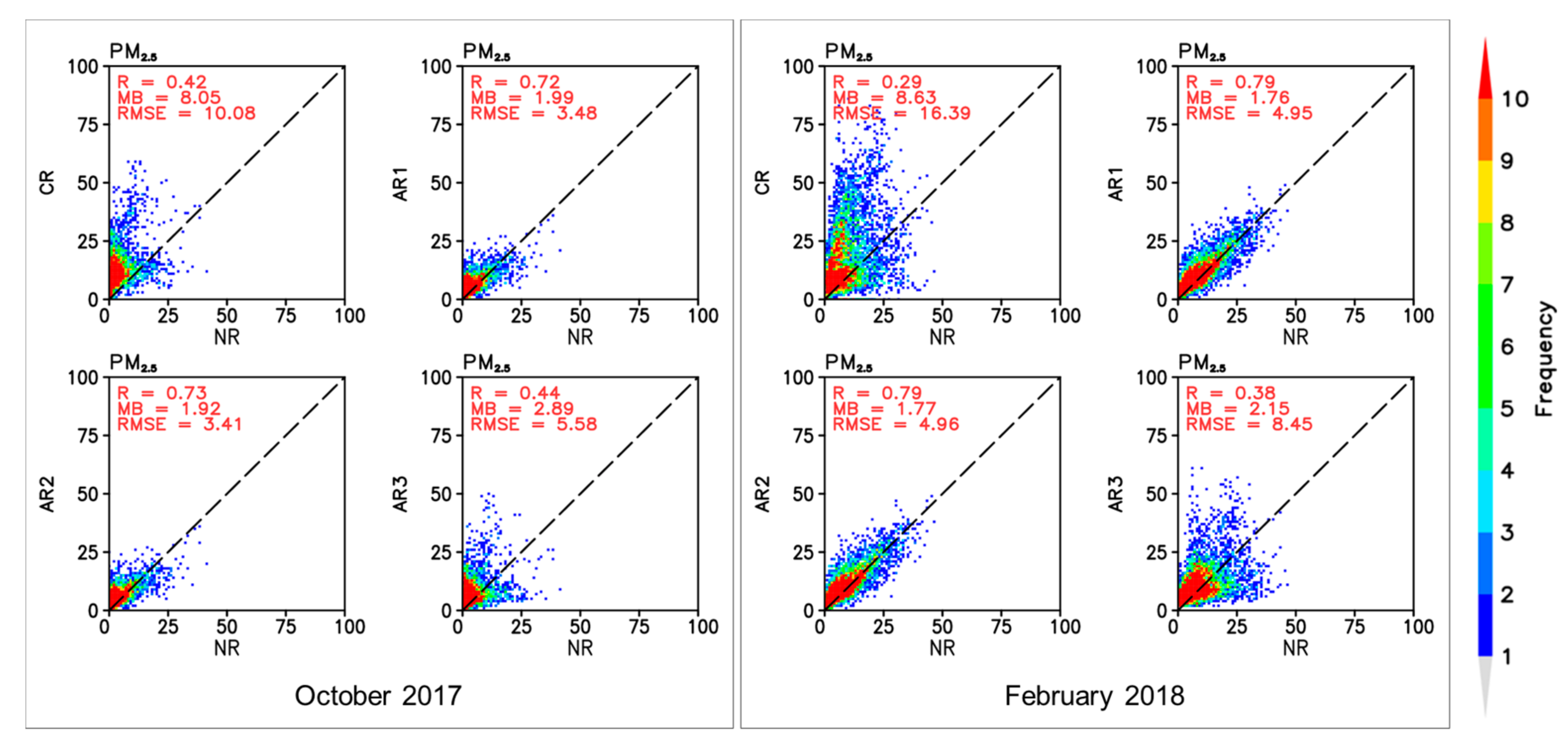
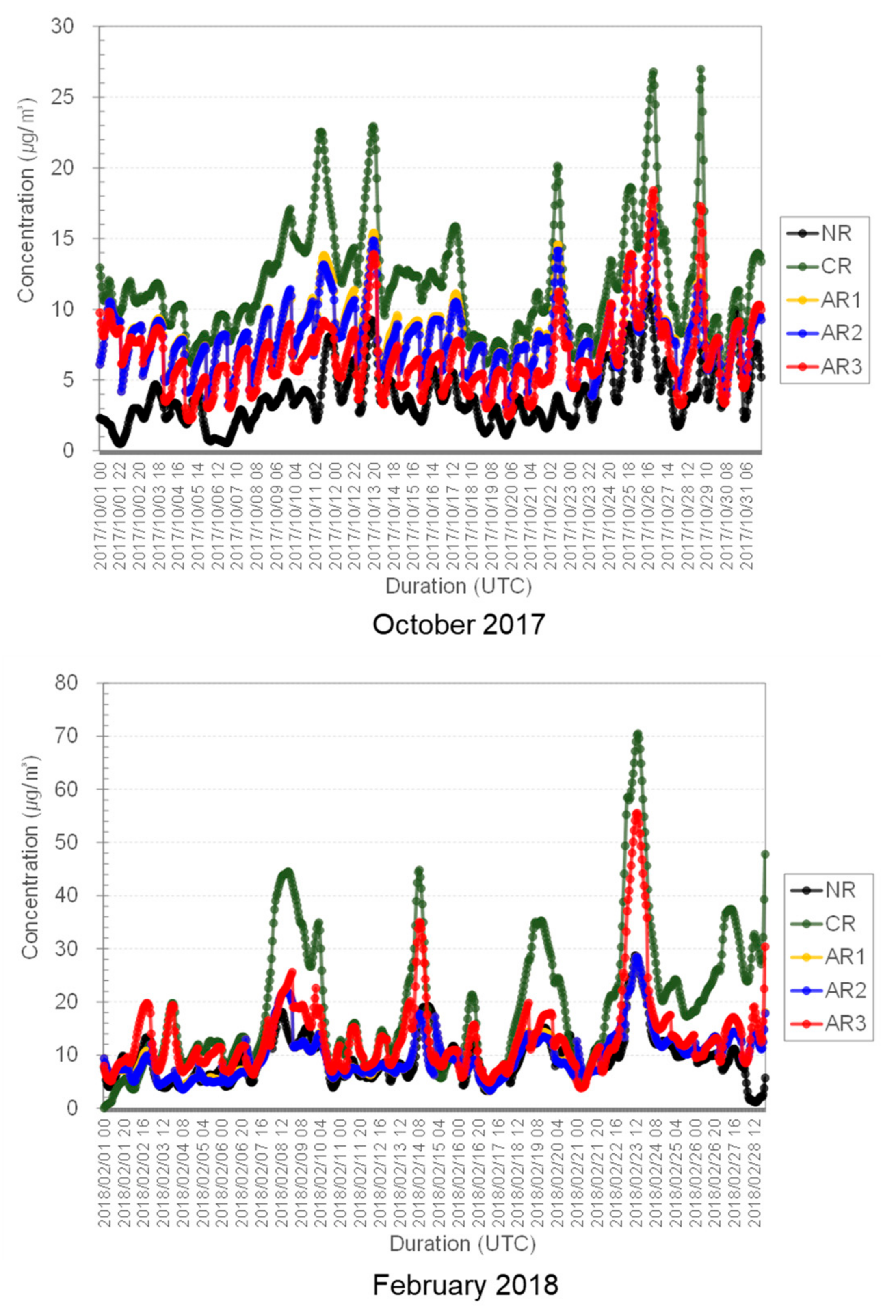
3.2. Potential Effects of New Observation Data

We attempted to quantify the impact of assimilating new surface PM and GEMS AOD data on the PM2.5 mass concentration forecasts on the Korean Peninsula through the intercomparison of four parallel simulation experiments. Among the four simulation experiments, one served as the control run (CR) that did not employ any DA and the other three served as the assimilation run (AR) group that employed 3DVAR DA using three sets of observation data. As shown in Table 1 and Figure 3, AR1 assimilated the surface PM2.5 and PM10 observation data from the 1306 current monitoring sites in China and South Korea, whereas AR2 assimilated the surface PM2.5 and PM10 observation from the current sites plus the virtual sites. AR3 performed the assimilation of solely GEMS AOD. We performed DA in one-way nested domains for Northeast Asia (D01) and the Korean Peninsula (D02) simultaneously at 6-h intervals in October 2017 and February 2018.
Figure 5 shows the distribution of the monthly averages of the individual PM2.5 forecasts of NR, CR, AR1, AR2, and AR3 in the Northeast Asia domain (D01) at 00:00 UTC. Together with the equivalent distribution on the Korean Peninsula, Figure 6 shows the distribution of the monthly averages of the respective deviations of the individual PM2.5 forecasts from the corresponding NR values. The NR results are supposed to be the observed concentrations (i.e., reference values).
The PM2.5 concentrations simulated by the CR were usually higher than those by the NR in the Gobi Desert, the inland areas of eastern China, Manchuria, and the Korean Peninsula in both October 2017 and February 2018 (Figure 5 and Figure 6). This large CR bias pattern for PM2.5 mass is partly attributed to the difference in the emission amounts used in WRF–Chem (i.e., CR) and CMAQ (i.e., NR). For example, the amounts of PM2.5, SO2, NOx, and NMVOC emissions in China that were used for the CR were 12.4, 33.2, 19, and 7.5% higher than those for the NR, respectively. It is also partly associated with the use of different aerosol modules in the NR and CR. Namely, the GOCART aerosol module in the CR internally calculated the dust occurrences in the desert area, whereas the AERO5 module in NR did not.
The assimilation of surface PM observation data (i.e., AR1 and AR2) exhibited less overestimation tendencies compared to the CR in China and on the Korean Peninsula and yield PM2.5 concentration forecasts that were closer to the NR results (Figure 5). Both AR2 (assimilating new observation data along with current observation data) and AR1 (assimilating just current observation data) appeared to provide almost similar PM2.5 concentration forecasts in D01, but there were differences in PM2.5 concentration forecast values in the Gobi Desert and certain areas of the Korean Peninsula. AR2 was found to further reduce the overpredictions in the Gobi Desert and North Korea compared to AR1 (Figure 5 and Figure 6). This demonstrates that adding 200 Gobi Desert and North Korean observation sites to the existing monitoring networks in China and the Korean Peninsula can improve PM2.5 prediction.
In addition to North Korea, parts of the Seoul Metropolitan Area (SMA) in South Korea experienced some improvement in the initial field of PM (Figure 6). The AR2 MB values across North Korea were smaller than the AR1 MB values, and the AR2 MB values in South Korea also somewhat decreased more than the AR1 MB in both October 2017 and February 2018. For example, a decrease in MB was observed across North Korea and in the western part of the SMA of South Korea. This improvement is partly attributed to the pollution characteristics of the SMA, which is constantly exposed to multiple sources of aerosol pollution from the local and surrounding areas. A previous study based on the Potential Source Density Function (PSDF) and backward trajectory analysis reported that coal burning for industrial processes in North Korea contributed to a high level of sulfate aerosols in the SMA during October 2015 [38]. Including the observation of such particulate pollution in North Korea in the current DA system reduced the bias errors of the PM2.5 forecasts in North Korea initially, and subsequently in the SMA of South Korea. When only the satellite AOD data were assimilated (AR3), PM forecasts improved to a certain level (Figure 5 and Figure 6), although the improvement in the initial field was less than that of the AR1 and AR2 cases.
Additional quantitative analyses to determine the model that achieved the most optimized improvement in the PM2.5 forecasts are presented in Figure 7, Figure 8 and Figure 9. A set of scatter plots presenting three statistics (R, MB, and RMSE) in Figure 7 help to determine which model offers relatively more optimized PM2.5 forecasts at 00:00 UTC across South Korea. For October 2017 (February 2018), the control run (CR) demonstrated a moderate correlation and the model’s overestimation and large errors were comparable with the fictitious observations (i.e., NR) at the surface monitoring sites in South Korea, as shown by the R, MB, and RMSE values of 0.42 (0.29), 8.05 µg/m3 (8.63 µg/m3), and 10.08 µg/m3 (16.39 µg/m3), respectively. However, the assimilation runs (AR1–AR3) showed significant improvements in the PM2.5 forecasts.
In October 2017 (February 2018), AR1 and AR2 at 00:00 UTC showed an increase of approximately 0.3 (0.5) in the correlation coefficient (r) value and a respective decrease of approximately 6.0 µg/m3 (6.8 µg/m3) and 6.6 µg/m3 (11.4 µg/m3) in the MB and RMSE values, respectively, compared to the CR, thereby indicating similar improvements for PM2.5 forecasts. The effect of the AR3 on the PM2.5 forecasts was slightly smaller than those of the other assimilation cases. AR3 showed an improvement in the PM2.5 forecasts at 00:00 UTC, an increase in the r value in October 2017 (February 2018) of approximately 0.02 (0.09), and a decrease in the MB and RMSE values in October 2017 (February 2018) of approximately 5.2 µg/m3 (6.5 µg/m3) and 4.5 µg/m3 (7.9 µg/m3), respectively. In short, these results suggest that the addition of new surface PM2.5 data and the sole use of GEMS AOD data are very effective in improving the initial field of PM air quality forecasts.
Figure 8 shows the time series of PM2.5 concentration forecasts (i.e., CR, ARs) and the corresponding observations (i.e., NR) for the experimental periods. The line graphs show the averaged hourly PM2.5 mass concentrations of NR and ARs across the 208 monitoring sites in South Korea.
All models, including the CR and ARs, captured the diurnal variations of the NR PM2.5 mass concentrations both in October 2017 and February 2018. The CR consistently and severely overpredicted, whereas the ARs tended to approach the observation levels. Assimilating the AOD produced (AR3) more optimized forecasts than assimilating the surface observations (AR1 and AR2) for most hours in October 2017, whereas assimilating the surface PM produced better forecasts than assimilating the AOD in February 2018. This pattern may be attributed to the different vertical distributions and source characteristics of surface PM and satellite AOD values [23,39,40]. For instance, the PM2.5 aerosols in the relatively warm season with fewer strong wind events (October 2017) are more likely to be distributed at higher mixing heights and influenced by slowly injected pollution from local sources, such as industrial activities and automobiles, in addition to the pollution in the medium-range transported by moderate winds. Moreover, PM2.5 tends to contribute to optical properties more than coarse size particles in the absence of dust events from the desert (e.g., [39]). Therefore, in this circumstance, the effect of assimilating the DA is likely to last longer because the DA of satellite AOD treats the total aerosol mass throughout the vertical column and maintains similar vertical structures [40]. In contrast with October, the PM2.5 aerosols in the cold season with frequent strong wind events (February 2018) are more likely to be distributed at lower mixing heights and influenced by the rapidly injected pollution from local sources, such as residential heating and automobiles, as well as the pollution in the long-range transported from the remote sources, including dust transported from the desert areas by strong winds. Therefore, the effect of the DA is likely to fade quickly when assimilating the surface PM observations [40].
Meanwhile, the forcasting skills of AR1 and AR2 showed a marginal difference, implying a small potential benefit for PM2.5 concentration forecasts on the Korean Peninsula due to the inclusion of the new surface observation data into the DA process. For example, AR1 overpredicted the hourly PM2.5 concentrations in October 2017 and February 2018 by factors of 2.7 and 1.26, respectively, and AR2 overpredicted the same concentrations by factors of 2.66 and 1.24, respectively. This represents reductions of approximately 1.1% and 1.4% in the overprediction rates of AR2 against AR1 in October 2017 and February 2018, respectively.
Figure 9 shows the percentage of improvement (PI) of the forecasting skill by the ARs (i.e., PI_AR1, PI_AR2, and PI_AR3), along with the forecasting errors of the base model (i.e., RMSE_CR) as a function of the time of day for October 2017 and February 2018.
The PI values in October 2017 show that assimilating the satellite AOD can significantly improve PM2.5 concentration forecasts more than assimilating the surface PM (i.e., greater values of PI_AR3 than of PI_AR1 or PI_AR2), whereas those from February 2018 show the opposite trend. The cause of these patterns is explained above (i.e., the different vertical distributions and source characteristics of the surface PM and satellite AOD values). In October 2017, the hourly RMSE values for the CR varied from 9.0 to 10.3 µg/m3. In this period, solely assimilating the current surface observation resulted in an approximately 63.7% (=PI_AR1) improvement in the PM2.5 concentration forecasts, assimilating the new surface observations along with the current surface observations resulted in an approximately 66.4% (=PI_AR_2) improvement, and solely assimilating the satellite AOD resulted in an approximately 68.4% (=PI_AR3) improvement. In February 2018, the hourly RMSE values for the CR varied from 13.4 to 15.8 µg/m3. In this period, only assimilating the current surface observations (AR1) or assimilating the new surface observations along with the current surface observations (AR2) improved forecasts by approximately 95.1% (i.e., PI_AR1 ≈ PI_AR2) and solely assimilating the satellite AOD improved forecasts by approximately 78.9% (=PI_AR3).
In October 2017, the PI values by AR1 and AR2 were the highest at approximately 88% and 89% at 00:00 UTC lead time, respectively, then decreased gradually until 08:00, increased for approximately 2 h, decreased again until 17:00, and then slowly increased. In contrast with AR1 and AR2, AR3 started at approximately 69.4% at 00:00 UTC lead time, which was approximately 1% higher than the average level, peaked at 06:00 (PI ~ 81%), decreased until 08:00, rebounded for 2 h, fell until 17:00, and then increased gradually. According to the comparison between the PI values of AR1 and AR2, including new observations from the Gobi Desert and North Korea in the current DA improved the PM2.5 concentration forecasts by 4.2% in October 2017.
The daily fluctuations of PI values calculated for AR1–AR3 in February 2018 were neither dynamic nor large compared to October 2017. The maximum PI values (~98%) by AR1 and AR2 were commonly derived in the early morning at 01:00 UTC (i.e., morning at 10:00 Korea Standard Time (KST)) lead time and the minimum values (~92%) in the early evening at 20:00 UTC (early morning at 5:00 KST) lead time. AR3 started at 90% at 00:00 UTC lead time, peaked at 02:00 (~90.5%), and then decreased gradually until the end time. In contrast with the October 2017 results, the effects of the new observations from the Gobi Desert and North Korea on the current DA were likely to be marginal in terms of improving the PM2.5 concentration forecasts in February 2018 (~0.05%).
Overall, PI values increased on average by approximately 45% upon assimilating the surface observations and by approximately 15% upon assimilating the satellite AOD in February 2018 compared to the cases in October 2017. According to the mean diurnal cycles of PI, the maxima-to-minima amplitudes for AR1, AR2, and AR3 were approximately 39.3, 36.3, and 21.8%, respectively, in October 2017 and approximately 6.0, 5.9, and 21.7%, respectively, in February 2018. Therefore, the effects of the DA on the PM2.5 concentration forecasts were larger and more stable in February 2018 than in October 2017.
Previous studies reported that the concurrent DA of both surface PM2.5 and satellite AOD observations produced more optimized forecasting scores than the DA of a single source of observation [28,40]. In future studies, both GEMS AOD and surface PM observations should be assimilated together over the testbed to examine the synergistic effect of assimilating different aerosol observations on PM2.5 forecasts.

4. Discussion

4.1. Nature Run Module

The NR in the current OSSE framework represented the temporal variations of the observed PM2.5 mass concentrations and showed significant underpredictions in the domain, especially in the suburban and remote areas (refer to the “Performance of the nature run” section). This bias should be reduced to ensure more realistic OSSE experiments [5,18]. The occurrence of bias and errors in the PM air quality simulations are associated with the complicated outer sources, such as the inaccurate emissions and meteorological data and ill-defined initial and boundary conditions for the model, as well as the model’s systematic bias associated with the inadequate representation of the atmospheric process [37,41]. In our case, one of the possible causes of the significant underpredictions is the outdated air quality model. The CMAQ model of the NR in the current OSSE framework is equipped with outdated modules for atmospheric chemistry and organic aerosol treatment compared to the recent versions of the CMAQ model (e.g., [42]). Therefore, to derive more realistic NR results in the OSSE framework, the CMAQ model employed in the current OSSE framework needs to be updated.

4.2. Data Scenario

The installation of 100 new observation sites in the Gobi Desert and in North Korea is hypothetical. This scenario was created solely to assess the feasibility of applying the developed OSSE framework. The model experiment showed that assimilating new PM data from the 100 Gobi Desert observation sites (i.e., AR2) was effective for PM2.5 forecasts in the desert area, but its effect on PM2.5 forecasts on the Korean Peninsula area was not clearly shown. This is likely due to the fact that there were no dust events severely influencing the air quality in South Korea at the time of modelling, such as Asian dust events [7]. For the period that Asian dust events severely affect the air quality in South Korea, this scenario is expected to contribute to improving PM2.5 forecasts on the Korean Peninsula.

4.3. Assimilation Run Module

We used the 3DVAR method for data assimilation in the current OSSE framework. The realistic estimates of background error covariance (BEC) are critical for an effective OSSE [5]. The 3DVAR method is computationally efficient and allows for multiple species in the analysis vector, but its weak point is the use of invariant BEC [28]. As mentioned in previous studies (e.g., [24,28,39]), we may consider introducing advanced DA methods, such as the ensemble Kalman filter (EnKF), which compute multivariate and flow-dependent BEC into the current OSSE framework. Computing power, which has continued to advance until recently, continues to open up opportunities for easing operational applications, even as the number of control variables increases in EnKF.

4.4. Data Assimilation System

The capability of the data assimilation system adopted in this study can be expanded by constantly adding new observation data from various sources [28]. Recently, a collaborative multidimensional atmospheric data-sharing platform (CMADS) was established in the National Strategic Project of Korea for fine particulate matter. It aims to integrate various air quality and meteorological datasets in Northeast Asia and to share them with relevant stakeholders, including the atmospheric environmental researchers and practitioner communities. GEMS data are also expected to be shared via this platform in the near future. Linking the current OSSE framework to the CMADS may allow for the application and evaluation of the system in various ways. For example, through the assimilation of the planetary boundary layer height (PBLH) derived by LiDAR observation shared in CMADS, we are likely to experience a certain level of improvement in the PM2.5 forecasts. This is because PBLH is one of the important determinants of the mixing volume of pollutants in the atmosphere ([39] and references therein). In addition to AOD, various gas-phase data observed by the GEMS can be regarded as important when used in the data assimilation system in the current OSSE framework.

5. Conclusions

We presented a recently developed OSSE framework and the results of a case study conducted over Northeast Asia. In the case study, we focused on the potential benefits of new PM observations from the Gobi Desert and North Korea (NEWPM) and new AOD observations from the GEMS (GEMS AOD) being added into the data assimilation with regard to the performance of the PM2.5 forecasts. Through the case study, we preliminarily tested and verified the utilization potential of the OSSE that we had established. For example, the performance statistics suggest that the concurrent assimilation of NEWPM and the PM data from current monitoring sites in China and South Korea can improve the PM2.5 concentration forecasts in South Korea by 66.4% on average for October 2017 (~95.1% on average for February 2018). In addition, assimilating even just the GEMS AOD could derive an approximately 68.4% improvement in the performance of the PM2.5 forecasts in South Korea for October 2017 (~78.9% for February 2018). We found that the OSSE framework could be a useful platform for preparing new air quality observations or data systems by providing the adequate evaluation of them in advance. Further studies over additional periods with new observation scenarios in other locations using bigger CR and AR boundaries and employing additional updated versions of the emissions database and model systems may be required; they would verify the feasibility of the current OSSE framework.

Author Contributions

Conceptualization, C.-K.S., K.J. and H.-K.K.; methodology, C.-K.S., S.L., M.-I.L. and H.-K.K.; software, S.L. and H.-K.K.; validation, K.-H.B. and H.-K.K.; formal analysis, S.L., K.-H.B. and H.-K.K.; investigation, S.L., K.-H.B. and H.-K.K.; writing—original draft preparation, H.-K.K.; writing—review and editing, C.-K.S., M.-I.L. and H.-K.K.; visualization, H.-K.K. and S.L.; supervision, C.-K.S.; project administration, C.-K.S. and K.J.; funding acquisition, C.-K.S. and K.J. All authors have read and agreed to the published version of the manuscript.

Funding

This work was supported by a grant from the National Institute of Environmental Research (NIER), funded by the Ministry of Environment (ME) of the Republic of Korea (NIER-2020-04-02-086 and NIER-2021-04-02-189). This research was also supported by the FRIEND (Fine Particle Research Initiative in East Asia Considering National Differences) Project through the National Research Foundation of Korea (NRF), funded by the Ministry of Science and ICT (grant no. 2020M3G1A1114615). In addition, this research was supported by Basic Science Research Program through the NRF funded by the Ministry of Education (2019R1I1A1A01045978).

Institutional Review Board Statement

Not applicable.

Informed Consent Statement

Not applicable.

Data Availability Statement

The data that support the findings of this study are available from the corresponding author (C.-K. Song), upon reasonable request.

Acknowledgments

The authors would like to thank E.-R. Kim at the Ulsan National Institute of Science and Technology (UNIST) for the preparation of the meteorological modeling data and also K.-H Kim at UNIST for helping with the installation of the WRF–Chem GSI system used in this study.

Conflicts of Interest

The authors declare no conflict of interest.

References

  1. World Health Organization Regional Office for Europe. Review of Evidence on Health Aspects of Air Pollution: REVIHAAP Project: Technical Report; World Health Organization; Regional Office for Europe: Copenhagen, Denmark, 2021. [Google Scholar]
  2. Carmichael, G.R.; Sandu, A.; Chai, T.; Daescu, D.N.; Constantinescu, E.M.; Tang, Y. Predicting air quality: Improvements through advanced methods to integrate models and measurements. J. Comput. Phys. 2008, 227, 3540–3571. [Google Scholar] [CrossRef]
  3. Kim, J.; Jeong, U.; Ahn, M.-H.; Kim, J.H.; Park, R.J.; Lee, H.; Song, C.H.; Choi, Y.-S.; Lee, K.-H.; Yoo, J.-M.; et al. New Era of Air Quality Monitoring from Space: Geostationary Environment Monitoring Spectrometer (GEMS). Bull. Am. Meteorol. Soc. 2020, 101, E1–E22. [Google Scholar] [CrossRef] [Green Version]
  4. Timmermans, R.; Lahoz, W.; Attié, J.-L.; Peuch, V.-H.; Edwards, D.; Eskes, H.; Builtjes, P. Observing System Simulation Experiments (OSSEs) for Air Quality Applications; Steyn, D.G., Chaumerliac, N., Eds.; Air Pollution Modeling and its Application XXIV; Springer International Publishing: Cham, Switzerland, 2016; pp. 581–585. [Google Scholar]
  5. Masutani, M.; Schlatter, T.W.; Errico, R.M.; Stoffelen, A.; Andersson, E.; Lahoz, W.; Woollen, J.S.; Emmitt, G.D.; Riishøjgaard, L.-P.; Lord, S.J. Observing System Simulation Experiments. In Data Assimilation: Making Sense of Observations; Lahoz, W., Khattatov, B., Menard, R., Eds.; Springer Berlin Heidelberg: Berlin/Heidelberg, Germany, 2010; pp. 647–679. [Google Scholar]
  6. Kim, I.S.; Lee, J.Y.; Wee, D.; Kim, Y.P. Estimation of the contribution of biomass fuel burning activities in North Korea to the air quality in Seoul, South Korea: Application of the 3D-PSCF method. Atmos. Res. 2019, 230, 104628. [Google Scholar] [CrossRef]
  7. Jung, M.-I.; Son, S.-W.; Kim, H.C.; Kim, S.-W.; Park, R.J.; Chen, D. Contrasting synoptic weather patterns between non-dust high particulate matter events and Asian dust events in Seoul, South Korea. Atmos. Environ. 2019, 214, 116864. [Google Scholar] [CrossRef]
  8. Filonchyk, M. Characteristics of the severe March 2021 Gobi Desert dust storm and its impact on air pollution in China. Chemosphere 2022, 287, 132219. [Google Scholar] [CrossRef] [PubMed]
  9. Byun, D.; Schere, K.L. Review of the Governing Equations, Computational Algorithms, and Other Components of the Models-3 Community Multiscale Air Quality (CMAQ) Modeling System. Appl. Mech. Rev. 2006, 59, 51–77. [Google Scholar] [CrossRef]
  10. Foley, K.M.; Roselle, S.J.; Appel, K.W.; Bhave, P.V.; Pleim, J.E.; Otte, T.L.; Mathur, R.; Sarwar, G.; Young, J.O.; Gilliam, R.C.; et al. Incremental testing of the Community Multiscale Air Quality (CMAQ) modeling system version 4.7. Geosci. Model Dev. 2010, 3, 205–226. [Google Scholar] [CrossRef] [Green Version]
  11. Chang, L.-S.; Cho, A.; Park, H.; Nam, K.; Kim, D.; Hong, J.-H.; Song, C.-K. Human-model hybrid Korean air quality forecasting system. J. Air Waste Manag. Assoc. 2016, 66, 896–911. [Google Scholar] [CrossRef] [PubMed] [Green Version]
  12. Lee, J.-J.; Lee, J.-B.; Kim, O.; Heo, G.; Lee, H.; Lee, D.; Kim, D.-G.; Lee, S.-D. Crop Residue Burning in Northeast China and Its Impact on PM2.5 Concentrations in South Korea. Atmosphere 2021, 12, 1212. [Google Scholar] [CrossRef]
  13. Woo, J.-H.; Choi, K.-C.; Kim, H.K.; Baek, B.H.; Jang, M.; Eum, J.-H.; Song, C.H.; Ma, Y.-I.; Sunwoo, Y.; Chang, L.-S.; et al. Development of an anthropogenic emissions processing system for Asia using SMOKE. Atmos. Environ. 2012, 58, 5–13. [Google Scholar] [CrossRef]
  14. Woo, J.-H.; Kim, Y.; Kim, H.-K.; Choi, K.-C.; Eum, J.-H.; Lee, J.-B.; Lim, J.-H.; Kim, J.; Seong, M. Development of the CREATE Inventory in Support of Integrated Climate and Air Quality Modeling for Asia. Sustainability 2020, 12, 7930. [Google Scholar] [CrossRef]
  15. Guenther, A.; Karl, T.; Harley, P.; Wiedinmyer, C.; Palmer, P.I.; Geron, C. Estimates of global terrestrial isoprene emissions using MEGAN (Model of Emissions of Gases and Aerosols from Nature). Atmos. Chem. Phys. 2006, 6, 3181–3210. [Google Scholar] [CrossRef] [Green Version]
  16. Larkin, N.K.; O’Neill, S.M.; Solomon, R.; Raffuse, S.; Strand, T.; Sullivan, D.C.; Krull, C.; Rorig, M.; Peterson, J.; Ferguson, S.A. The BlueSky smoke modeling framework. Int. J. Wildland Fire 2009, 18, 906–920. [Google Scholar] [CrossRef] [Green Version]
  17. Van der Werf, G.R.; Randerson, J.T.; Giglio, L.; van Leeuwen, T.T.; Chen, Y.; Rogers, B.M.; Mu, M.; van Marle, M.J.E.; Morton, D.C.; Collatz, G.J.; et al. Global fire emissions estimates during 1997–2016. Earth Syst. Sci. Data 2017, 9, 697–720. [Google Scholar] [CrossRef] [Green Version]
  18. Timmermans, R.M.A.; Lahoz, W.A.; Attié, J.L.; Peuch, V.H.; Curier, R.L.; Edwards, D.P.; Eskes, H.J.; Builtjes, P.J.H. Observing System Simulation Experiments for air quality. Atmos. Environ. 2015, 115, 199–213. [Google Scholar] [CrossRef]
  19. Chin, M.; Rood, R.B.; Lin, S.-J.; Müller, J.-F.; Thompson, A.M. Atmospheric sulfur cycle simulated in the global model GOCART: Model description and global properties. J. Geophys. Res. Atmos. 2000, 105, 24671–24687. [Google Scholar] [CrossRef]
  20. Purser, R.J.; Wu, W.-S.; Parrish, D.F.; Roberts, N.M. Numerical Aspects of the Application of Recursive Filters to Variational Statistical Analysis. Part I: Spatially Homogeneous and Isotropic Gaussian Covariances. Mon. Weather Rev. 2003, 131, 1524–1535. [Google Scholar] [CrossRef]
  21. Purser, R.J.; Wu, W.-S.; Parrish, D.F.; Roberts, N.M. Numerical Aspects of the Application of Recursive Filters to Variational Statistical Analysis. Part II: Spatially Inhomogeneous and Anisotropic General Covariances. Mon. Weather Rev. 2003, 131, 1536–1548. [Google Scholar] [CrossRef]
  22. Wu, W.-S.; Purser, R.J.; Parrish, D.F. Three-Dimensional Variational Analysis with Spatially Inhomogeneous Covariances. Mon. Weather Rev. 2002, 130, 2905–2916. [Google Scholar] [CrossRef] [Green Version]
  23. Jiang, Z.; Liu, Z.; Wang, T.; Schwartz, C.S.; Lin, H.-C.; Jiang, F. Probing into the impact of 3DVAR assimilation of surface PM10 observations over China using process analysis. J. Geophys. Res. Atmos. 2013, 118, 6738–6749. [Google Scholar] [CrossRef]
  24. Liu, Z.; Liu, Q.; Lin, H.-C.; Schwartz, C.S.; Lee, Y.-H.; Wang, T. Three-dimensional variational assimilation of MODIS aerosol optical depth: Implementation and application to a dust storm over East Asia. J. Geophys. Res. Atmos. 2011, 116, 399–411. [Google Scholar] [CrossRef] [Green Version]
  25. Pagowski, M.; Liu, Z.; Grell, G.A.; Hu, M.; Lin, H.C.; Schwartz, C.S. Implementation of aerosol assimilation in Gridpoint Statistical Interpolation (v. 3.2) and WRF-Chem (v. 3.4.1). Geosci. Model Dev. 2014, 7, 1621–1627. [Google Scholar] [CrossRef] [Green Version]
  26. Parrish, D.F.; Derber, J.C. The National Meteorological Center’s Spectral Statistical-Interpolation Analysis System. Mon. Weather Rev. 1992, 120, 1747–1763. [Google Scholar] [CrossRef]
  27. Elbern, H.; Strunk, A.; Schmidt, H.; Talagrand, O. Emission rate and chemical state estimation by 4-dimensional variational inversion. Atmos. Chem. Phys. 2007, 7, 3749–3769. [Google Scholar] [CrossRef] [Green Version]
  28. Schwartz, C.S.; Liu, Z.; Lin, H.-C.; McKeen, S.A. Simultaneous three-dimensional variational assimilation of surface fine particulate matter and MODIS aerosol optical depth. J. Geophys. Res. Atmos. 2012, 117, 110–117. [Google Scholar] [CrossRef]
  29. Choi, M.; Kim, J.; Lee, J.; Kim, M.; Park, Y.J.; Holben, B.; Eck, T.F.; Li, Z.; Song, C.H. GOCI Yonsei aerosol retrieval version 2 products: An improved algorithm and error analysis with uncertainty estimation from 5-year validation over East Asia. Atmos. Meas. Tech. 2018, 11, 385–408. [Google Scholar] [CrossRef] [Green Version]
  30. Kim, G.; Lee, S.; Im, J.; Song, C.-K.; Kim, J.; Lee, M.-i. Aerosol data assimilation and forecast using Geostationary Ocean Color Imager aerosol optical depth and in-situ observations during the KORUS-AQ observing period. GIScience Remote Sens. 2021, 58, 1175–1194. [Google Scholar] [CrossRef]
  31. Grell, G.A.; Peckham, S.E.; Schmitz, R.; McKeen, S.A.; Frost, G.; Skamarock, W.C.; Eder, B. Fully coupled “online” chemistry within the WRF model. Atmos. Environ. 2005, 39, 6957–6975. [Google Scholar] [CrossRef]
  32. Janssens-Maenhout, G.; Dentener, F.; Van Aardenne, J.; Monni, S.; Pagliari, V.; Orlandini, L.; Klimont, Z.; Kurokawa, J.; Akimoto, H.; Ohara, T.; et al. EDGAR-HTAP: A harmonized Gridded Air Pollution Emission Dataset Based on National Inventories; European Commission, Joint Research Centre, Institute for Environment and Sustainability: Luxemburg, 2012; pp. 1–40. Available online: https://publications.jrc.ec.europa.eu/repository/handle/JRC68434 (accessed on 15 October 2020).
  33. Hand, J.L.; Copeland, S.A.; Day, D.E.; Dillner, A.M.; Indresand, H.; Malm, W.C.; McDade, C.E.; Moore, C.T.; Pitchford, M.L.; Schichtel, B.A.; et al. IMPROVE (Interagency Monitoring of Protected Visual Environments): Spatial and Seasonal Patterns and Temporal Variability of Haze and Its Constituents in the United States; 2011. Available online: http://vista.cira.colostate.edu/Improve/spatial-and-seasonal-patterns-and-temporal-variability-of-haze-and-its-constituents-in-the-united-states-report-v-june-2011/ (accessed on 29 January 2019).
  34. Carter, W.P. Implementation of the SAPRC-99 Chemical Mechanism into the Models-3 Framework; United States Environmental Protection Agency: Washington, DC, USA, 2000; pp. 1–101. Available online: https://intra.cert.ucr.edu/~carter/pubs/s99mod3.pdf (accessed on 30 January 2021).
  35. Rio, M.H.; Santoleri, R. Improved global surface currents from the merging of altimetry and Sea Surface Temperature data. Remote Sens. Environ. 2018, 216, 770–785. [Google Scholar] [CrossRef]
  36. Arnold, C.P.; Dey, C.H. Observing-Systems Simulation Experiments: Past, Present, and Future. Bull. Am. Meteorol. Soc. 1986, 67, 687–695. [Google Scholar] [CrossRef] [Green Version]
  37. Boylan, J.W.; Russell, A.G. PM and light extinction model performance metrics, goals, and criteria for three-dimensional air quality models. Atmos. Environ. 2006, 40, 4946–4959. [Google Scholar] [CrossRef]
  38. Kim, N.K.; Kim, I.S.; Song, I.H.; Park, S.M.; Lim, H.B.; Kim, Y.P.; Shin, H.J.; Lee, J.Y. Temporal variation of sulfate concentration in PM2.5 and major factors enhancing sulfate concentration in the atmosphere of Seoul, Korea. Air Qual. Atmos. Health 2021, 14, 985–999. [Google Scholar] [CrossRef]
  39. Wang, Y.; Sartelet, K.N.; Bocquet, M.; Chazette, P.; Sicard, M.; D’Amico, G.; Léon, J.F.; Alados-Arboledas, L.; Amodeo, A.; Augustin, P.; et al. Assimilation of lidar signals: Application to aerosol forecasting in the western Mediterranean basin. Atmos. Chem. Phys. 2014, 14, 12031–12053. [Google Scholar] [CrossRef] [Green Version]
  40. Werner, M.; Kryza, M.; Guzikowski, J. Can Data Assimilation of Surface PM2.5 and Satellite AOD Improve WRF-Chem Forecasting? A Case Study for Two Scenarios of Particulate Air Pollution Episodes in Poland. Remote Sens. 2019, 11, 2364. [Google Scholar] [CrossRef] [Green Version]
  41. Russell, A.; Dennis, R. NARSTO critical review of photochemical models and modeling. Atmos. Environ. 2000, 34, 2283–2324. [Google Scholar] [CrossRef]
  42. Wyat Appel, K.; Napelenok, S.; Hogrefe, C.; Pouliot, G.; Foley, K.M.; Roselle, S.J.; Pleim, J.E.; Bash, J.; Pye, H.O.T.; Heath, N.; et al. Overview and Evaluation of the Community Multiscale Air Quality (CMAQ) Modeling System Version 5.2; Springer: Cham, Switzerland, 2018; pp. 69–73. [Google Scholar]
Figure 1. The schematic for the OSSE framework developed in the study.
Remotesensing 14 00389 g001
Figure 2. The Observing System Simulation Experiments (OSSE) testbed domain. The NR boundary in blue shows the domain for the nature run; the CR and AR boundaries in red indicate the domain for control and assimilation runs, respectively.
Remotesensing 14 00389 g002
Figure 3. The schematic of the OSSE scenarios.
Remotesensing 14 00389 g003
Figure 4. The NR results for (a) October 2017 and (b) February 2018. Top figures: the distribution of the monthly averages of the simulated PM2.5 mass concentrations in NR. Mid-figures: the correlation coefficients between the NR PM2.5 concentration and the ground-observed PM2.5 concentration at the surface monitoring sites. Bottom figures: the mean bias of the simulated PM2.5 mass concentrations.
Remotesensing 14 00389 g004
Figure 5. The distribution of the average PM2.5 concentrations in East Asia for the NR and ARs (i.e., AR1, AR2, and AR3) at 00:00 universal time coordinated (UTC) from October 2017 to February 2018 (unit: µg/m3).
Remotesensing 14 00389 g005
Figure 6. The distribution of the average PM2.5 concentrations on the Korean Peninsula for the NR, ARs, and the AR mean bias against the NR PM2.5 at 00:00 UTC from October 2017 to February 2018 (unit: µg/m3).
Remotesensing 14 00389 g006
Figure 7. Scatter plots for the AR PM2.5 mass concentrations (unit: µg/m3) and the corresponding NR PM2.5 at 208 monitoring sites in South Korea at 00:00 UTC from October 2017 to February 2018.
Remotesensing 14 00389 g007
Figure 8. The time series of the simulated results for PM2.5 of NR, CR, and Ars at 208 monitoring sites in South Korea in October 2017 and February 2018.
Remotesensing 14 00389 g008
Figure 9. The diurnal variations of the percentage improvement (PI) of PM2.5 forecasts by ARs along with the RMSE of the CR (RMSE_CR) at the 208 monitoring sites in South Korea for October 2017 and February 2018.
Remotesensing 14 00389 g009
Table 1. The settings for the nature run (NR), control run (CR), and data assimilation run (AR) in the OSSE.
Air Quality Model SettingInput Observation for DA
NRCMAQ version 4.7.1 with
  • horizontal resolution: a single domain of a 9 km × 9 km resolution system (438,806 grids)
  • vertical layers: 25
  • gas-phase chemistry scheme: SAPRC99
  • aerosol scheme: AERO5 Ψ
  • meteorology: output of WRF version 3.9.1
  • emissions: CREATE2015 for anthropogenic sources
Not used
CRWRF–Chem version 3.9.1 model with
  • horizontal resolution: a mother domain of a 27 km × 27 km resolution system (22,225 grids) and son domain of a 9 km × 9 km resolution system (13,192 grids)
  • vertical layers: 31
  • gas-phase chemistry scheme: MOZART version 4
  • aerosol scheme: GOCART
  • emissions: EDGAR–HTAP for anthropogenic sources and MEGAN for biogenic sources
Not used
AR 1Same as CR but for 6-hourly data assimilation
  • data assimilation method: GSI 3D-Var
PM10 and PM2.5 from NR at real station location (1306 sites)
AR 2 Same as AR1 and AR3 but for the input observation for DAPM10 and PM2.5 from NR at the locations of the real monitoring sites and 100 sites over the Gobi Desert area and 100 sites over the North Korean non-forest area (1506 sites)
AR 3Same as AR1 and AR2 but for the input observation for DAAOD from NR consistent with time and spatial resolution of the GEMS satellite (746,115 locations)
[34] and Ψ [10].
Publisher’s Note: MDPI stays neutral with regard to jurisdictional claims in published maps and institutional affiliations.

