
VENµS-Derived NDVI and REIP at Different View Azimuth Angles


1
The Remote Sensing Laboratory, French Associates Institute for Agriculture and Biotechnology of Drylands, Jacob Blaustein Institutes for Desert Research, Ben-Gurion University of the Negev, Sede Boqer Campus, Beersheba 8455902, Israel
2
The Robert H. Smith Institute of Plant Sciences and Genetics in Agriculture, The Hebrew University of Jerusalem, Rehovot 7610001, Israel
*
Author to whom correspondence should be addressed.
Remote Sens. 2022, 14(1), 184; https://doi.org/10.3390/rs14010184
Submission received: 30 November 2021
/
Revised: 15 December 2021
/
Accepted: 28 December 2021
/
Published: 1 January 2022
(This article belongs to the Special Issue VENµS Image Processing Techniques and Applications)
Abstract
:The bidirectional reflectance distribution function (BRDF) is crucial in determining the quantity of reflected light on the earth’s surface as a function of solar and view angles (i.e., azimuth and zenith angles). The Vegetation and ENvironment monitoring Micro-Satellite (VENµS) provides a unique opportunity to acquire data from the same site, with the same sensor, with almost constant solar and view zenith angles from two (or more) view azimuth angles. The present study was aimed at exploring the view angles’ effect on the stability of the values of albedo and of two vegetation indices (VIs): the normalized difference vegetation index (NDVI) and the red-edge inflection point (REIP). These products were calculated over three polygons representing urban and cultivated areas in April, June, and September 2018, under a minimal time difference of less than two minutes. Arithmetic differences of VIs and a change vector analysis (CVA) were performed. The results show that in urban areas, there was no difference between the VIs, whereas in the well-developed field crop canopy, the REIP was less affected by the view azimuth angle than the NDVI. Results suggest that REIP is a more appropriate index than NDVI for field crop studies and monitoring. This conclusion can be applied in a constellation of satellites that monitor ground features simultaneously but from different view azimuth angles.
1. Introduction
The Vegetation and ENvironment monitoring Micro-Satellite (VENµS) is an earth observation space mission jointly developed, manufactured, and operated by the National Centre for Space Studies (CNES) and the Israel Space Agency (ISA) [1]. The satellite, launched in August 2017, crosses the equator at around 10:30 a.m. Coordinated Universal Time (UTC) through a sun-synchronous orbit at a 720-km height with a 98° inclination. The scientific objective of VENμS is to frequently acquire images on 160 preselected sites with a two-day revisit time, a high spatial resolution of 5 m, and 12 narrow bands, ranging from 424 to 909 nm, including four red-edge bands (Table 1). This band setting was designed to characterize vegetation status, monitor water quality in coastal areas and inland waters, and estimate the aerosol optical depth and the water vapor content of the atmosphere. Duplication of the red band enables the creation of digital terrain models (DTMs) of the earth’s surface and clouds. To observe specific sites within its 27-km swath, the satellite can be tilted up to 30 degrees along and across track. Uniquely, the preselected sites are always observed with constant view azimuth and zenith angles.
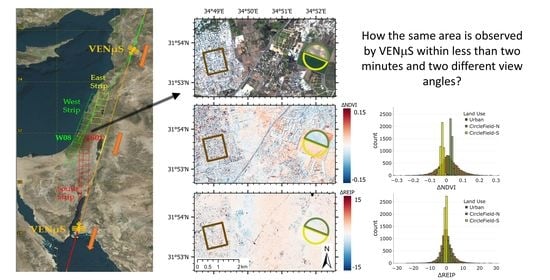
Figure 1a depicts the footprint of the three VENμS strips over Israel and their corresponding view azimuth angles. The west strip, composed of 12 tiles named W01–W12, was the first area covered by the satellite during its descending orbit at around 8:30 UTC (Table 2). The duration of the image capturing was 36 s in a forward view mode. After a few seconds of maneuvering, while the camera was in standby mode, the satellite measured the five tiles of the east strip (i.e., E01–E05) in a backward view mode for 20 s. Finally, the 10 tiles of the south strip (i.e., S01–S10) were covered in 30 s in the backward view mode. The time needed to acquire all 27 tile images over the Israeli scientific sites was 161 s. According to the spatial coverage of these strips, there are some overlapping zones between the west and the south strips. The overlapping images can be used to explore the effect of the view azimuth angle on the spectral reflectance acquired from space as one component of the bidirectional reflectance distribution function (BRDF) [2]. The differences between the other three components, i.e., view zenith angle, solar azimuth angle, and solar zenith angle, are assumed to be minimal and, therefore, neglected.
The view angle and sun elevation, along with their combination, are well known and have been explored from various spaceborne platforms and observation heights [3,4,5]. To the best of our knowledge, the VENμS satellite is the only publicly available platform that allows data collection from the same site, with the same sensor, from two (or more) view azimuth angles within minutes. The current study was aimed at exploring the view angle’s effect on the stability of the values of vegetation indices (VIs) and albedo due to changes in the view angle under the minimum time gap. It was hypothesized that the view angle would affect VI values and that this effect would vary between ground features. The two selected VIs were the normalized difference vegetation index (NDVI) [6], which is easily available and frequently applied, and the red-edge inflection point (REIP), which is unique to sensors with four red-edge bands (e.g., VENμS and Sentinel-2 [7]). The REIP showed better sensitivity to several vegetation properties, such as leaf area index (LAI) [8] and chlorophyll and nitrogen contents [9]. The albedo characterizes the brightness of ground features affected by the BRDF, which was used as a reference for each VI.
2. Materials and Methods
2.1. VENµS Data Collection
Images, available on a designated website (https://venus.bgu.ac.il/venus/), were taken from November 2017 to the end of October 2020. Three levels of VENµS scientific products were available, free of charge, to the scientific community: Level 1 (L1), Level 2 (L2), and Level 3 (L3). The L1 product included the top of the atmosphere reflectance with a spatial resolution of 5 m, whereas L2 and L3 contained surface reflectance for a single day and for a 10-day time composite, respectively. To reduce storage space, the L2 and L3 data were generated at a 10-m resolution after atmospheric corrections performed by the MACCS-ATCOR Joint Algorithm (i.e., MAJA [10]). Note that recently, the entire archive has been reprocessed to provide surface reflectance images at a 5-m resolution. In this study, single-day L2 data were used from three selected dates: 18 April, 27 June, and 11 September 2018.
2.2. Study Area
The study area was located in the overlapping zone of the west strip’s tile W08 and the south strip’s tile S01 (Figure 1b). This 188.31 km2 area contained different types of land-use and land-cover categories: urban, vegetation, soil, vineyards, orchards, and water, amongst others. Table 2 shows the acquisition times in UTC and the BRDF components of the W08 and S01 tiles on 18 April 2018. It can be seen that tile S01 was acquired 1 min and 56 s after tile W08, and the difference in the view azimuth is notable, i.e., more than 150 degrees. Furthermore, image W08 was acquired in a forward direction, while S01 was in a backward direction. The current study focused on a representative section in the northern part of the overlap zone, including three polygons (Figure 1c). Two polygons in the center comprise irrigated fields in a cultivated area, representing agricultural soil and vegetation surfaces (hereafter named CircleField-N and CircleField-S). A third polygon included an urban area (hereafter named Urban) and is an example of a heterogeneous surface. To fulfill the study goal, three clear-sky days were used in different seasons of the year (i.e., 18 April, 27 June, and 11 September 2018). The CircleField-N area had bare soil on the first date, developed corn plants on the second date, and bare soil on the third. The CircleField-S area had developed chickpea plants on the first date, ready-to-harvest dry chickpea plants on the second date, and bare soil on the third.
2.3. Vegetation Indices and Albedo
To explore the effect of the view zenith angle across the study sites, two VIs were selected, the normalized difference vegetation index (NDVI) [6] and the red-edge inflection point (REIP) [7,8,9]:
where is the relative reflectance of the subscript wavelength expressed in nm. The NDVI is a well-known and frequently used VI that can be calculated from many satellite sensors, while the REIP is less known and rarely used because the four needed bands are not available in many spaceborne sensors. These bands are available in the VENμS and Sentinel-2 satellites. The NDVI and the REIP were simulated and discussed for VENμS resampled bands to estimate leaf area index by [8] and, in the current study, were calculated from space to allow a comparison of their values under different view angles. In the current study, the NDVI was calculated with bands B7 and B10, and the REIP was calculated with bands B7, B8, B9, and B10 (Table 1).
Additionally, the albedo was calculated as follows [11]:
where and are the surface reflectance and the bandwidth, in nm, for band i, respectively. All VENµS bands were involved in this process.
2.4. Pixel Subtraction
The VIs’ value change was calculated as measured by the VENμS satellite from two different view azimuth angles. First, the indices were calculated for all pixels in the overlap zone for each of the two tiles, and later, the former tile value (W08) was subtracted from the later one (S01):
where VI is the vegetation index (Equations (1) and (2)), and subscript S01 and W08 indicate the relevant tile.
2.5. Change Vector Analysis
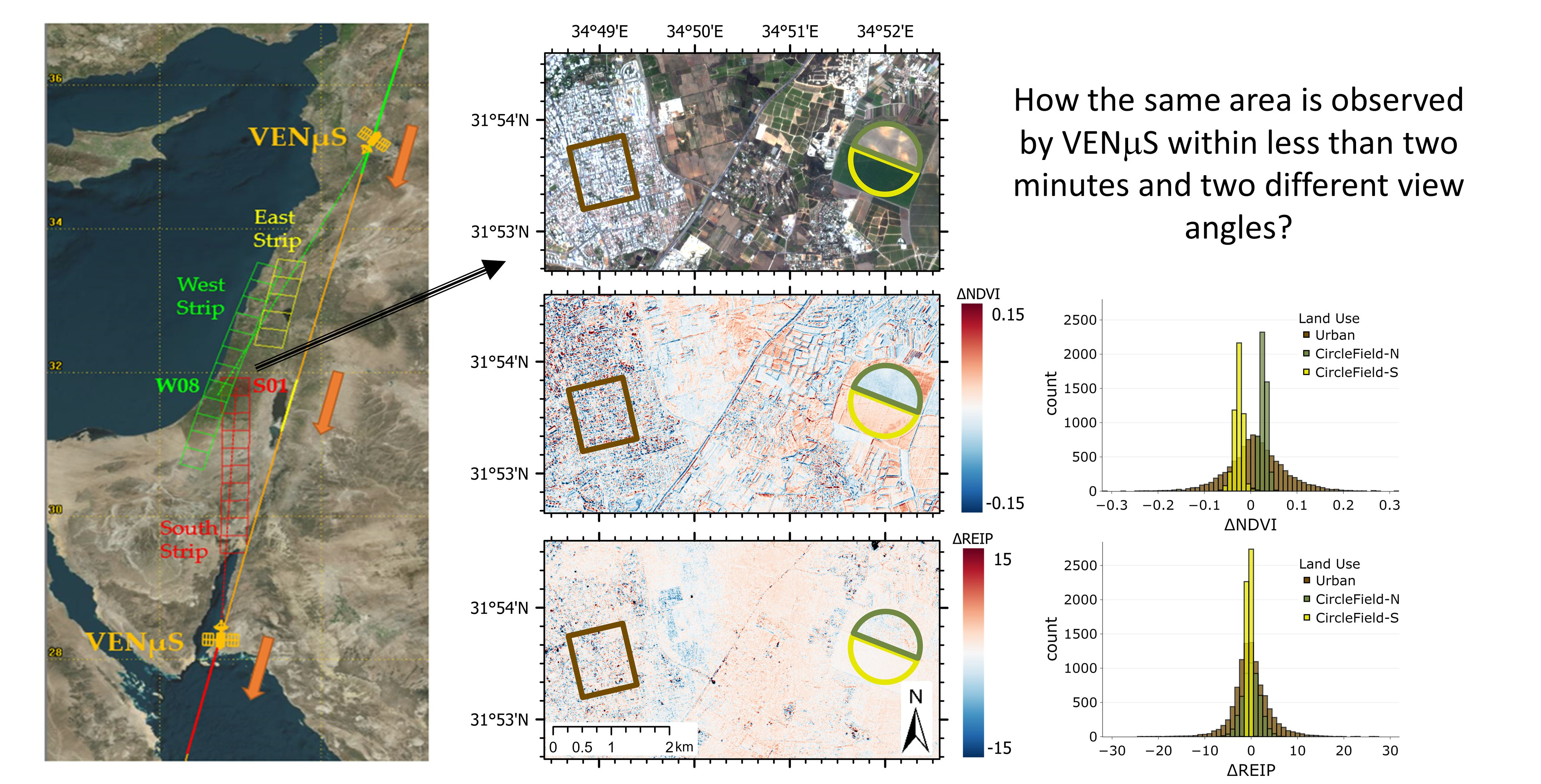
The change vector analysis (CVA) is a robust methodology for detecting multivariant changes from two or more spectral bands, spectral features, or biophysical indicators (e.g., spectral indices) associated with the pixel of an image [12]. In the current study, CVA was computed to measure the magnitude and direction of the change in NDVI and REIP (Equations (1) and (2)) versus the albedo α (Equation (3)), between the two tiles (i.e., S01 with respect to W08), and across all pixels in the overlap zone. The VIs represent vegetated pixels since the high index value indicates more biomass, while the albedo represents bare light-colored soil since higher values indicate a more exposed non-vegetated surface. First, these variables were computed in the overlap zone, and then, the VIs were normalized to values between 0 and 1 to eliminate the bias of the CVA magnitude due to the dynamic range of each index. Finally, the CVA was performed pixel-by-pixel between the reference dataset W08 and the target dataset S01. The output of the CVA consists of the change vector (CV) magnitude (Equation (5)) and the change direction (θ, Equation (6)). The CV magnitude, |CV|, is the Euclidean distance of the vector between the reference and the target datasets:
where nVI is the normalized vegetation index, and α is the albedo. A threshold was defined in order to distinguish between changed and unchanged pixels (i.e., noise). One standard deviation (1-STD) was selected as a threshold [13,14,15]. The direction of the change vector is represented by the angle θ, as depicted in Figure 2:
where nVI is the normalized vegetation index, α is the albedo, and subscript S01 and W08 indicate the relevant tile.
3. Results and Discussion
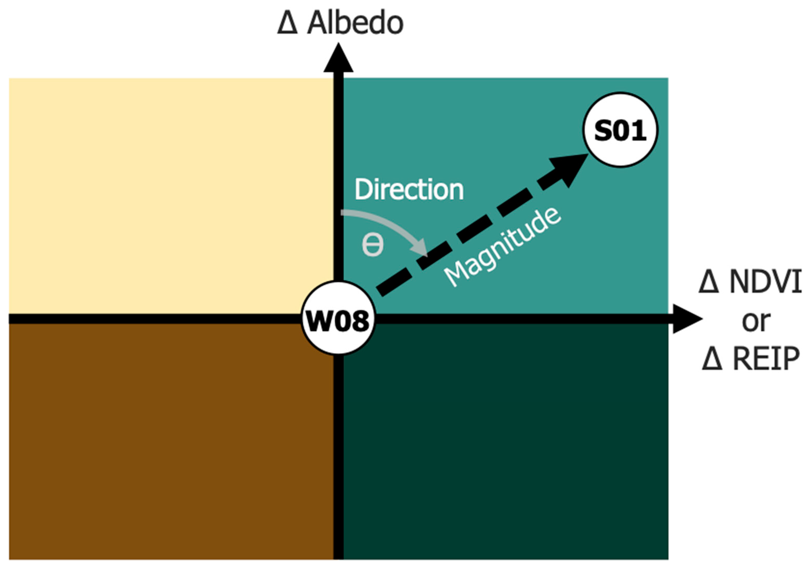
To explore the view azimuth angle’s effect on the spectral reflectance, the change in the VIs (Equation (4)) was examined in three selected polygons (Figure 3a). The NDVI pixel subtraction (∆NDVI) of the two tiles (S01–W08) showed the distinct difference as a function of the land use (Figure 3b,c). For example, on April 18, the southern half-circle of the chickpea crop field (i.e., CircleField-S, yellow-colored polygon in Figure 3a) was characterized by negative values of ∆NDVI, while the post-sowing bare soil of the northern half-circle of the corn crop field (i.e., CircleField-N, green-colored polygon in Figure 3a) was characterized by positive ∆NDVI values. Similarly, most northern corn fields showed negative values, while the southern dry chickpea field showed values distributed around zero on June 27. On September 11, bare soil was found in both cultivated fields with ∆NDVI values distributed similarly at around zero difference. On all the selected dates, the relatively homogeneous half-circle fields were characterized by narrow distributions (yellow and green-colored bars in Figure 3c). In contrast, the inhomogeneous urban area (i.e., Urban) was characterized by a wider distribution of ∆NDVI (brown-colored bars in Figure 3c). In accordance with its relatively low seasonal variability, the urban area was characterized by similar distributions for all selected dates with no negative–positive dominance. Examination of the ∆REIP values (Figure 3d,e) for the exact dates and polygons also showed distinct differences. Areas with dominant vegetation, such as the chickpea field’s southern half-circle (yellow-colored polygon on April 18) or the corn field’s northern half-circle (green-colored polygon on June 27), showed nearly zero differences (Figure 3e). On the other hand, bare soil and urban areas consistently showed wider distributions and larger differences. The ∆Albedo values (Figure 3f,g) showed a mainly positive change as expected based on the solar and view angles (Table 2).
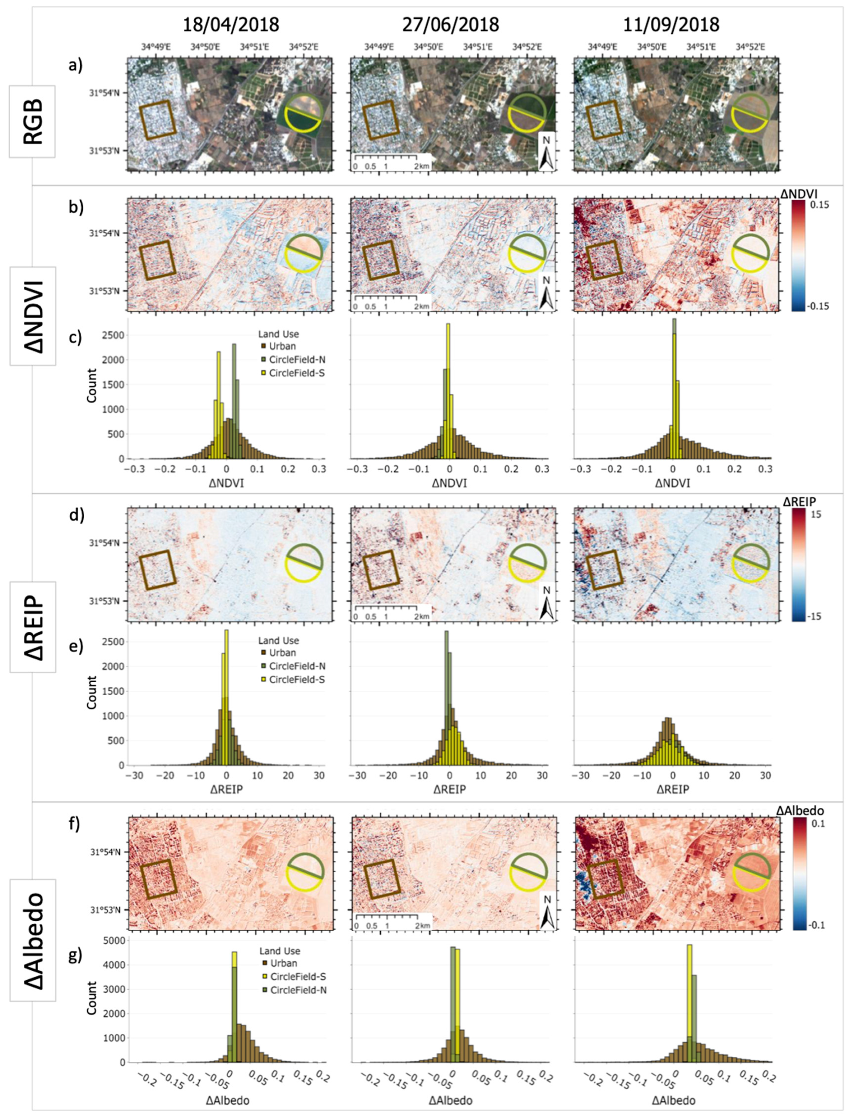
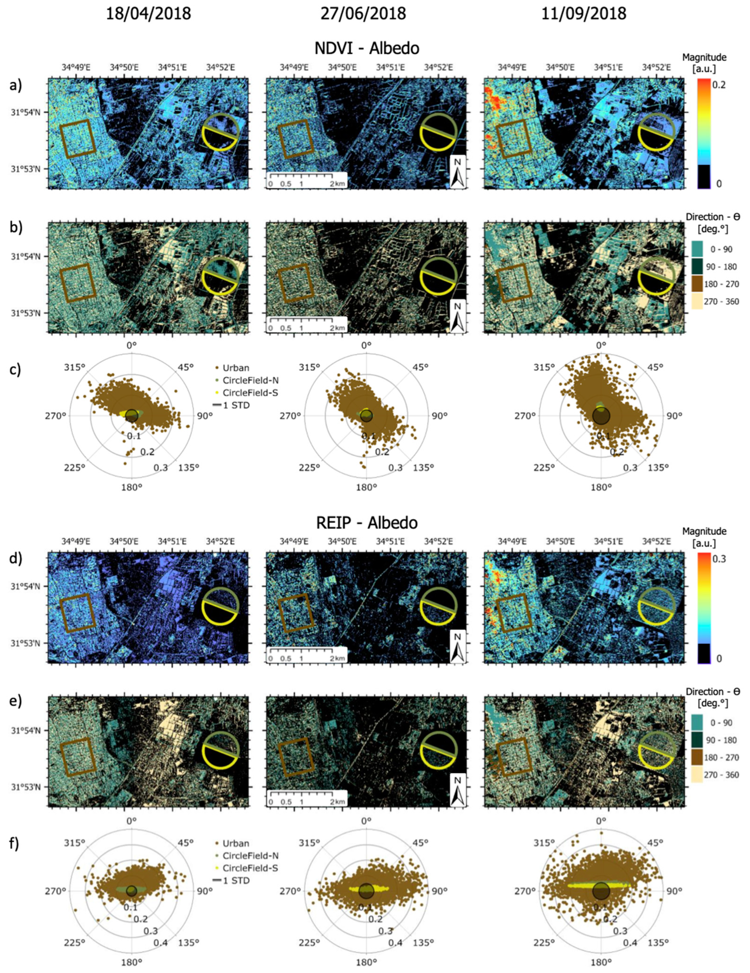
The CVA magnitude for the NDVI-albedo combination showed that pixels with a CV magnitude (Figure 4a) lower than the threshold (1-STD) were considered as no-change pixels and colored black. The same threshold was also used for the REIP-albedo combination (Figure 4d). The urban area and the bare soil in the circle fields showed relatively large magnitude changes, while areas such as field crops or dry matter showed no change. Therefore, the NDVI values, as obtained by VENμS, of vegetative areas were less affected by the view azimuth angle than those of soil areas. Nevertheless, dry standing vegetative biomass (i.e., CircleField-S on June 27) areas or bare soil fields a relatively long time after harvest (i.e., CircleField-S on September 11) had a magnitude below the threshold (i.e., showed no change). Figure 4a shows the CV magnitudes as a function of land use, similar to the direction in Figure 4b. In addition, the polar plots in Figure 4c illustrate both the magnitude and the direction changes for each polygon of interest on the selected dates. Following the positive changes in albedo for the two half-circle crop fields (Figure 3f,g), their direction continued to be on the upper part (i.e., positive ∆Albedo). In contrast, the urban area was characterized by negative and positive changes in albedo, with some patterns connecting these changes of ∆Albedo with changes in ∆NDVI (Figure 4c).
The similarities between NDVI-albedo and REIP-albedo (Figure 4) included the dominant positive ∆Albedo in the crop field areas vs. positive or negative ∆Albedo in the urban area and the distinct narrow distribution of ∆REIP in the vegetative crop field areas vs. the wider distribution of ∆REIP in the bare soil, dry matter, and urban areas. It was found that those areas of nearly zero ∆REIP (i.e., the half-circle crop fields with vegetation) also had magnitude values smaller than the 1-STD threshold. Therefore, the change in the view azimuth angle did not affect the REIP in these areas as obtained by VENμS.
The results obtained in the present work, based on the VENµS mission, suggest that the REIP index was less affected by the view azimuth angle than the NDVI, thus making it a better tool for analyzing and comparing the spectral response in vegetative areas measured at different azimuth angles. In addition to the VENµS mission, described in Section 1, the MultiSpectral Imager (MSI) onboard the Sentinel-2 mission captures the reflected light signal at the four red-edge bands [8,9] with no charge for users.
In recent years, several space agencies and companies have advanced the concept of satellite constellations that consist of mini/micro/nano space systems for earth observation [16]. Such large fleets of satellites strive to enable global monitoring of the earth with many images while minimizing the revisit time. This formation includes satellites that simultaneously point to the same earth target but with different view azimuth angles. Therefore, the findings of the current study are crucial for processing vegetation properties in the forthcoming era of satellite constellations.
4. Conclusions
The current study aimed to explore the effect of the view azimuth angle on two VENμS-derived VI values (i.e., NDVI and REIP) used in image processing for agricultural applications. The effect of the view azimuth angle on the NDVI value for field crops was more significant than its effect on REIP, while in the urban area, there was no difference between the VIs. The main finding is that in a fully developed field crop canopy, the REIP was less affected by the view azimuth angle than the NDVI. This finding provides additional evidence for preferring the REIP to the NDVI, which is more affected by high above-ground biomass. Currently, as the four red-edge bands are freely available by VENμS as well as Sentinel-2, the REIP has demonstrated its advantage in the view azimuth angle for field crops, in addition to its higher sensitivity to increasing vegetation biomass. Therefore, the REIP, when applicable, is recommended for field crop studies and monitoring. Specifically, the findings of the current study are crucial for processing vegetation properties in the forthcoming era of satellite constellations.
Author Contributions
M.S.: methodology, software, data curation, writing, and visualization; Y.T.: methodology, software, data curation, writing, and visualization; A.K.: methodology, writing, and funding acquisition; I.H.: conceptualization, methodology, data curation, writing, and funding acquisition. All authors have read and agreed to the published version of the manuscript.
Funding
This study was partially supported by the Hebrew University of Jerusalem’s Intramural Research Fund in Career Development.
Institutional Review Board Statement
Not applicable.
Informed Consent Statement
Not applicable.
Data Availability Statement
The satellite imagery used are available on VENμS site https://venus.bgu.ac.il/venus/ (accessed on 15 December 2021).
Conflicts of Interest
The authors declare no conflict of interest.
References
- Dedieu, G.; Karnieli, A.; Hagolle, O.; Jeanjean, H.; Cabot, F.; Ferrier, P.; Yaniv, Y. A Joint Israeli–French Earth Observation Scientific Mission with High Spatial and Temporal Resolution Capabilities. In Proceedings of the 4th ESA CHRIS/Proba Work, ESRIN, Frascati, Italy, 19–21 September 2006; pp. 19–21. [Google Scholar]
- Schaepman-Strub, G.; Schaepman, M.E.; Painter, T.H.; Dangel, S.; Martonchik, J.V. Reflectance quantities in optical remote sensing—definitions and case studies. Remote Sens. Environ. 2006, 103, 27–42. [Google Scholar] [CrossRef]
- Roy, D.P.; Zhang, H.K.; Ju, J.; Gomez-Dans, J.L.; Lewis, P.E.; Schaaf, C.B.; Sun, Q.; Li, J.; Huang, H.; Kovalskyy, V. A general method to normalize Landsat reflectance data to nadir BRDF adjusted reflectance. Remote Sens. Environ. 2016, 176, 255–271. [Google Scholar] [CrossRef] [Green Version]
- Mueller, N.; Lewis, A.; Roberts, D.; Ring, S.; Melrose, R.; Sixsmith, J.; Lymburner, L.; McIntyre, A.; Tan, P.; Curnow, S.; et al. Water observations from space: Mapping surface water from 25 years of Landsat imagery across Australia. Remote Sens. Environ. 2016, 174, 341–352. [Google Scholar] [CrossRef] [Green Version]
- Liu, Y.; Hill, M.; Zhang, X.; Wang, Z.; Richardson, A.D.; Hufkens, K.; Filippa, G.; Baldocchi, D.D.; Ma, S.; Verfaillie, J.; et al. Using data from Landsat, MODIS, VIIRS and PhenoCams to monitor the phenology of California oak/grass savanna and open grassland across spatial scales. Agric. For. Meteorol. 2017, 237–238, 311–325. [Google Scholar] [CrossRef]
- Tucker, C.J. Red and photographic infrared linear combinations for monitoring vegetation. Remote Sens. Environ. 1979, 8, 127–150. [Google Scholar] [CrossRef] [Green Version]
- Martimort, P.; Fernandez, V.; Kirschner, V.; Isola, C.; Meygret, A. Sentinel-2 MultiSpectral imager (MSI) and calibra-tion/validation. Int. Geosci. Remote Sens. Symp. 2012, 6999–7002. [Google Scholar]
- Herrmann, I.; Pimstein, A.; Karnieli, A.; Cohen, Y.; Alchanatis, V.; Bonfil, D.J. LAI assessment of wheat and potato crops by VENμS and Sentinel-2 bands. Remote Sens. Environ. 2011, 115, 2141–2151. [Google Scholar] [CrossRef]
- Clevers, J.G.P.W.; Gitelson, A.A. Remote estimation of crop and grass chlorophyll and nitrogen content using red-edge bands on Sentinel-2 and -3. Int. J. Appl. Earth Obs. Geoinf. 2013, 23, 344–351. [Google Scholar] [CrossRef]
- Hagolle, O.; Huc, M.; Desjardins, C.; Auer, S.; Richter, R. MAJA Algorithm Theoretical Basis Document. Development 2017, 1–39. Available online: http://tully.ups-tlse.fr/olivier/maja_atbd/raw/master/atbd_maja.pdf (accessed on 15 December 2021).
- Robinove, C.J.; Chavez, P.S.; Gehring, D.; Holmgren, R. Arid land monitoring using Landsat albedo difference images. Remote. Sens. Environ. 1981, 11, 133–156. [Google Scholar] [CrossRef]
- Johnson, R.D.; Kasischke, E.S. Change vector analysis: A technique for the multispectral monitoring of land cover and condition. Int. J. Remote Sens. 1998, 19, 411–426. [Google Scholar] [CrossRef]
- Karnieli, A.; Qin, Z.; Wu, B.; Panov, N.; Yan, F. Spatio-Temporal Dynamics of Land-Use and Land-Cover in the Mu Us Sandy Land, China, Using the Change Vector Analysis Technique. Remote Sens. 2014, 6, 9316–9339. [Google Scholar] [CrossRef] [Green Version]
- Zanchetta, A.; Bitelli, G.; Karnieli, A. Monitoring desertification by remote sensing using the Tasselled Cap transform for long-term change detection. Nat. Hazards 2016, 83, 223–237. [Google Scholar] [CrossRef]
- Bayarjargal, Y.; Karnieli, A.; Bayasgalan, M.; Khudulmur, S.; Gandush, C.; Tucker, C.J. A comparative study of NO-AA-AVHRR derived drought indices using change vector analysis. Remote Sens. Environ. 2006, 105, 9–22. [Google Scholar] [CrossRef]
- Curzi, G.; Modenini, D.; Tortora, P. Large Constellations of Small Satellites: A Survey of Near Future Challenges and Missions. Aerospace 2020, 7, 133. [Google Scholar] [CrossRef]
Figure 1.
(a) Spatial distribution of the three VENμS strips over Israel; (b) the overlapping zone of the VENμS tiles, located in the S01 (red) and W08 (green); (c) the three selected polygons of Urban (brown), CircleField-N (green), and CircleField-S (yellow).
Figure 1.
(a) Spatial distribution of the three VENμS strips over Israel; (b) the overlapping zone of the VENμS tiles, located in the S01 (red) and W08 (green); (c) the three selected polygons of Urban (brown), CircleField-N (green), and CircleField-S (yellow).

Figure 2.
A graphical scheme illustrates how the change vector analysis (CVA) equations were applied to calculate the change magnitude and change direction (angle θ) for the VENμS-derived NDVI, REIP, and albedo and between the reference tile W08 and the target tile S01. The change magnitude is represented by the distance of S01 from W08, and the change direction is represented by the degree angle in the range between 0° and 360°. The direction value range is divided into four main classes of 90° (i.e., quadrant).

Figure 3.
∆NDVI, ∆REIP, and ∆Albedo maps and the value distributions for the three land-use polygons (i.e., Urban, CircleField-N, and CircleField-S) colored in brown, green, and yellow, respectively, and the three dates (i.e., 18 April, 27 June, and 11 September 2018). (a) VENμS RGB images acquired on the three dates, including the three land-use polygons. (b,d), and (f) ∆VI maps (Equation (4)) for the same area of interest and three selected dates, showing the spatial variability of positive (red color) and negative (blue color) difference values. (c,e,g) Histogram plots showing the distribution of the ∆VI values for each date and each land-use polygon. The color of each bin matches the color of its polygon.

Figure 4.
Change vector analysis (CVA) of NDVI-albedo (a,b), and (c) and REIP-albedo (d,e), and (f) for the three dates (i.e., 18 April, 27 June, and 11 September 2018). (a,d) Magnitude maps calculated by Equation (6). (b,e) Direction maps calculated by Equation (6); the colors are based on Figure 2. Pixels colored in black have magnitude values smaller than the one standard deviation (1-STD) threshold, determined as no-change pixels. (c,f) Polar plots illustrating the changed magnitude (i.e., distance from the center) and changed direction (i.e., degree angle between 0° and 360°) value distribution for the three dates and the three polygons (i.e., Urban, CircleField-N, CircleField-S), colored in brown, green, and yellow, respectively. The color of each point matches the color of its polygon; black circles mark the areas below 1-STD-presented as black (a,b,d,e).


Table 1.
VENµS satellite band information.
| Bands | Central Wavelength (nm) | Bandwidth (nm) | Main Application |
|---|---|---|---|
| B1 | 423.9 | 40 | Atmospheric Correction, Water |
| B2 | 446.9 | 40 | Aerosols, Clouds |
| B3 | 491.9 | 40 | Atmospheric Correction, Water |
| B4 | 555.0 | 40 | Land |
| B5 | 619.7 | 40 | Vegetation Indices |
| B6 | 619.7 | 40 | DEM, Image Quality |
| B7 | 666.2 | 30 | Red Edge |
| B8 | 702.0 | 24 | Red Edge |
| B9 | 741.1 | 16 | Red Edge |
| B10 | 782.2 | 16 | Red Edge |
| B11 | 861.1 | 40 | Vegetation Indices |
| B12 | 908.7 | 20 | Water Vapor |
B stands for band; DEM stands for digital elevation model.
Table 2.
BRDF components and acquisition time for tiles W08 (west strip) and S01 (south strip) on 18 April, 27 June, and 11 September 2018.
Table 2.
BRDF components and acquisition time for tiles W08 (west strip) and S01 (south strip) on 18 April, 27 June, and 11 September 2018.
| W08 | S01 | |||||
|---|---|---|---|---|---|---|
| Apr. 18 | Jun. 27 | Sep. 11 | Apr. 18 | Jun. 27 | Sep. 11 | |
| View zenith angle (deg) | 35.29 | 35.54 | 35.29 | 30.10 | 30.31 | 30.13 |
| View azimuth angle (deg) | 25.88 | 27.16 | 25.77 | 179.15 | 177.41 | 179.26 |
| Solar zenith angle (deg) | 26.21 | 18.17 | 31.14 | 25.85 | 17.63 | 30.86 |
| Solar azimuth angle (deg) | 138.39 | 112.50 | 146.93 | 139.78 | 113.76 | 148.21 |
| Acquisition time (UTC) | 08:31:27 | 08:31:43 | 8:32:58 | 08:33:23 | 08:33:40 | 08:34:54 |
Publisher’s Note: MDPI stays neutral with regard to jurisdictional claims in published maps and institutional affiliations. |
© 2022 by the authors. Licensee MDPI, Basel, Switzerland. This article is an open access article distributed under the terms and conditions of the Creative Commons Attribution (CC BY) license (https://creativecommons.org/licenses/by/4.0/).
Share and Cite
MDPI and ACS Style
Salvoldi, M.; Tubul, Y.; Karnieli, A.; Herrmann, I. VENµS-Derived NDVI and REIP at Different View Azimuth Angles. Remote Sens. 2022, 14, 184. https://doi.org/10.3390/rs14010184
AMA Style
Salvoldi M, Tubul Y, Karnieli A, Herrmann I. VENµS-Derived NDVI and REIP at Different View Azimuth Angles. Remote Sensing. 2022; 14(1):184. https://doi.org/10.3390/rs14010184
Chicago/Turabian StyleSalvoldi, Manuel, Yaniv Tubul, Arnon Karnieli, and Ittai Herrmann. 2022. "VENµS-Derived NDVI and REIP at Different View Azimuth Angles" Remote Sensing 14, no. 1: 184. https://doi.org/10.3390/rs14010184
Note that from the first issue of 2016, this journal uses article numbers instead of page numbers. See further details here.