
Detection of Larch Forest Stress from Jas’s Larch Inchworm (Erannis jacobsoni Djak) Attack Using Hyperspectral Remote Sensing

 ,
,
Abstract
: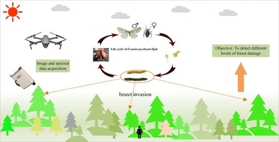
1. Introduction
2. Materials and Methods
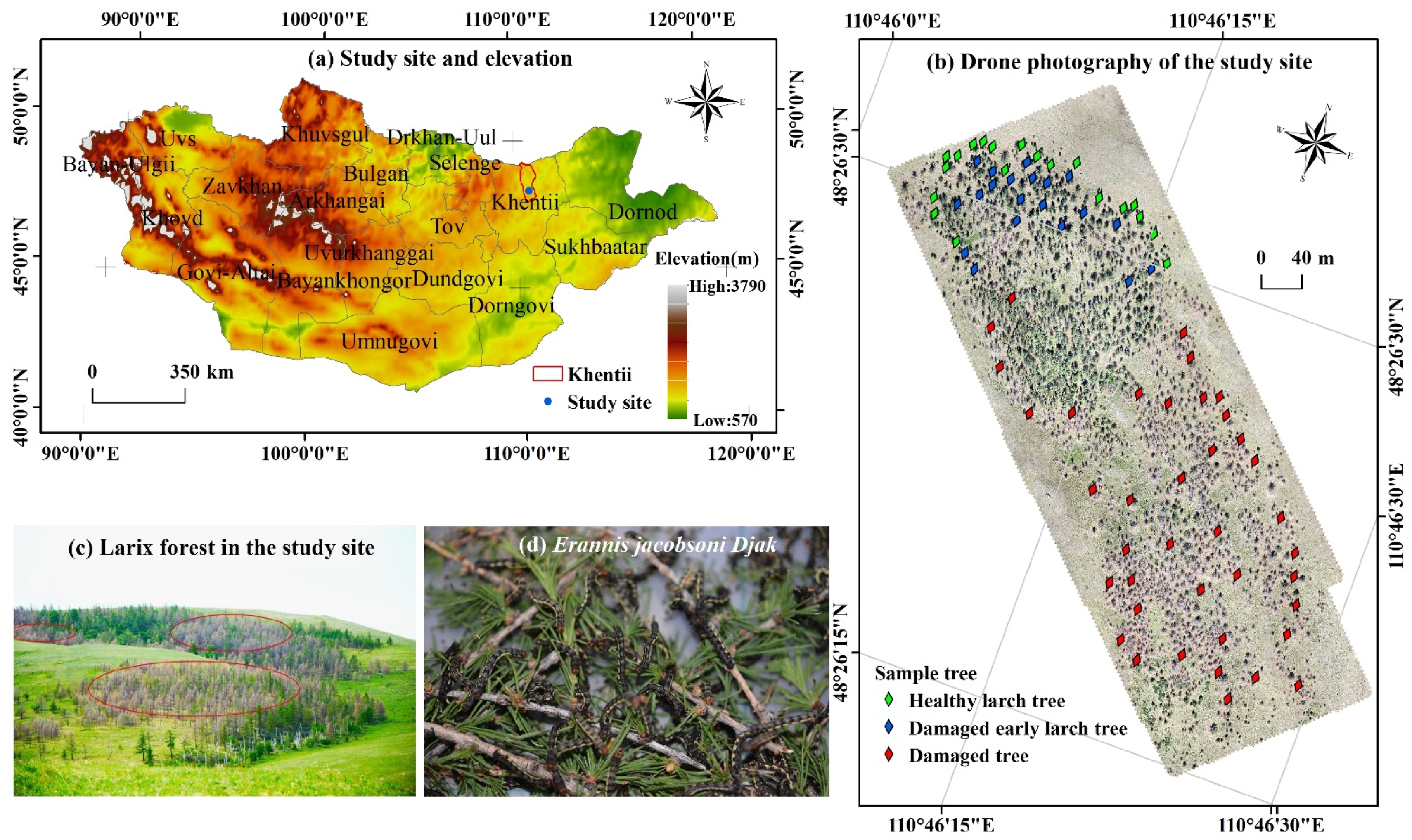
2.1. Study Area
2.2. Data Preparation and Preprocessing
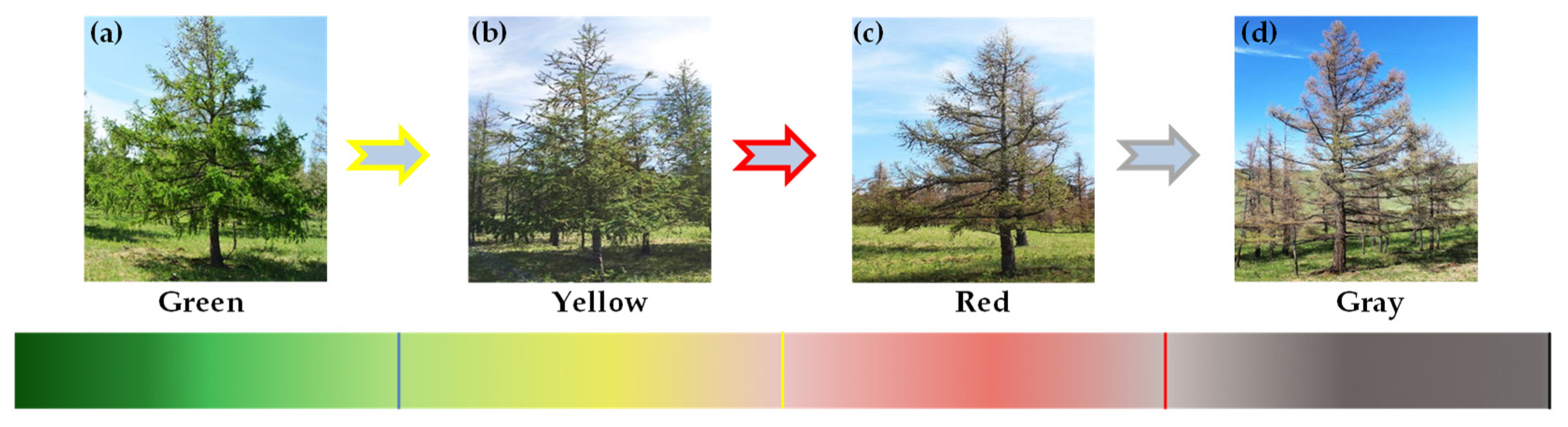
2.2.1. Selection of Sample Trees
2.2.2. Hyperspectral Data Collection and Preprocessing
2.2.3. Data Collection and Preprocessing of Biochemical Components
- (1)
- Chlorophyll content data
- (2)
- Water content data
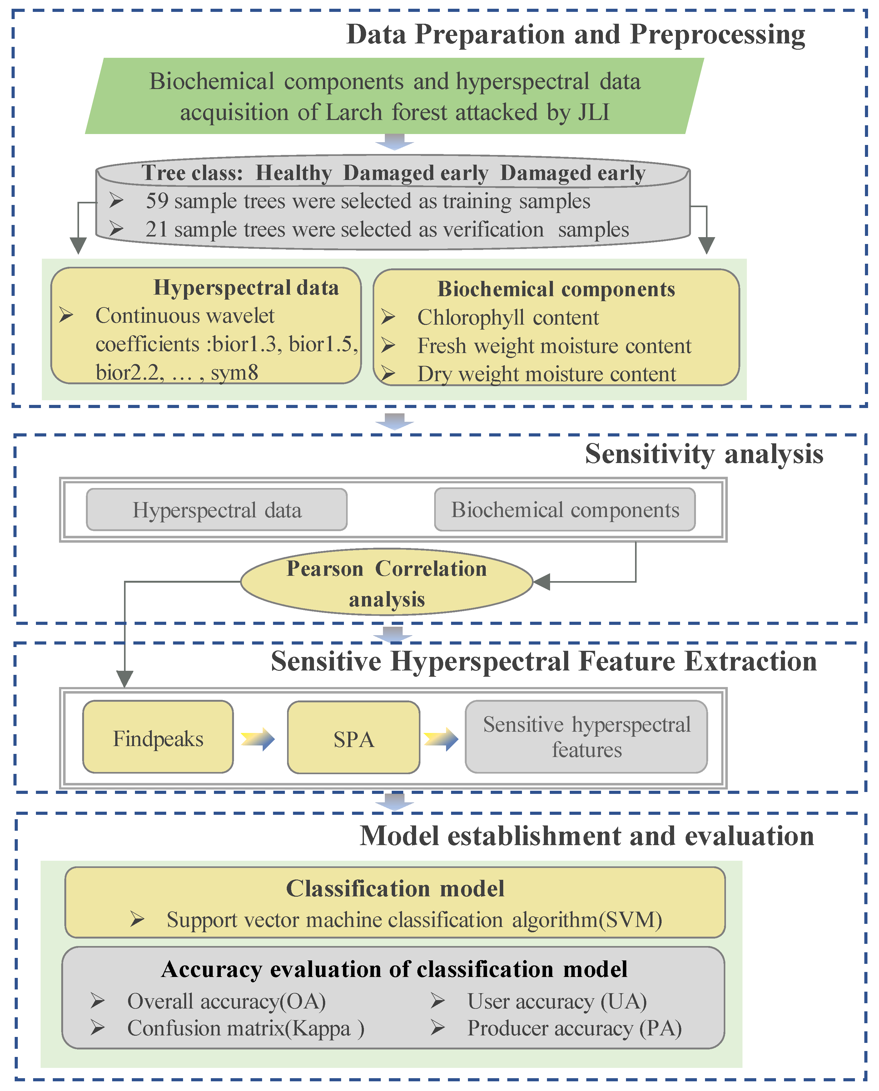
2.3. Method
2.3.1. Sensitivity Analysis
2.3.2. Sensitive Hyperspectral Feature Extraction
2.3.3. Model Establishment and Evaluation
3. Results
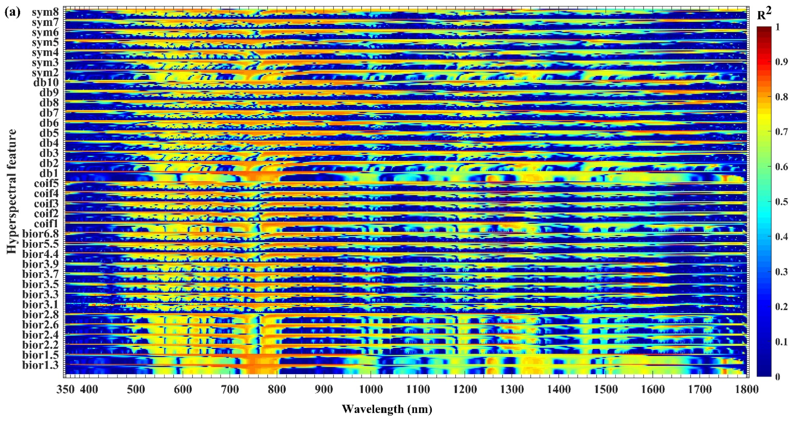
3.1. Sensitivity Analysis of Hyperspectral Features to Biochemical Components
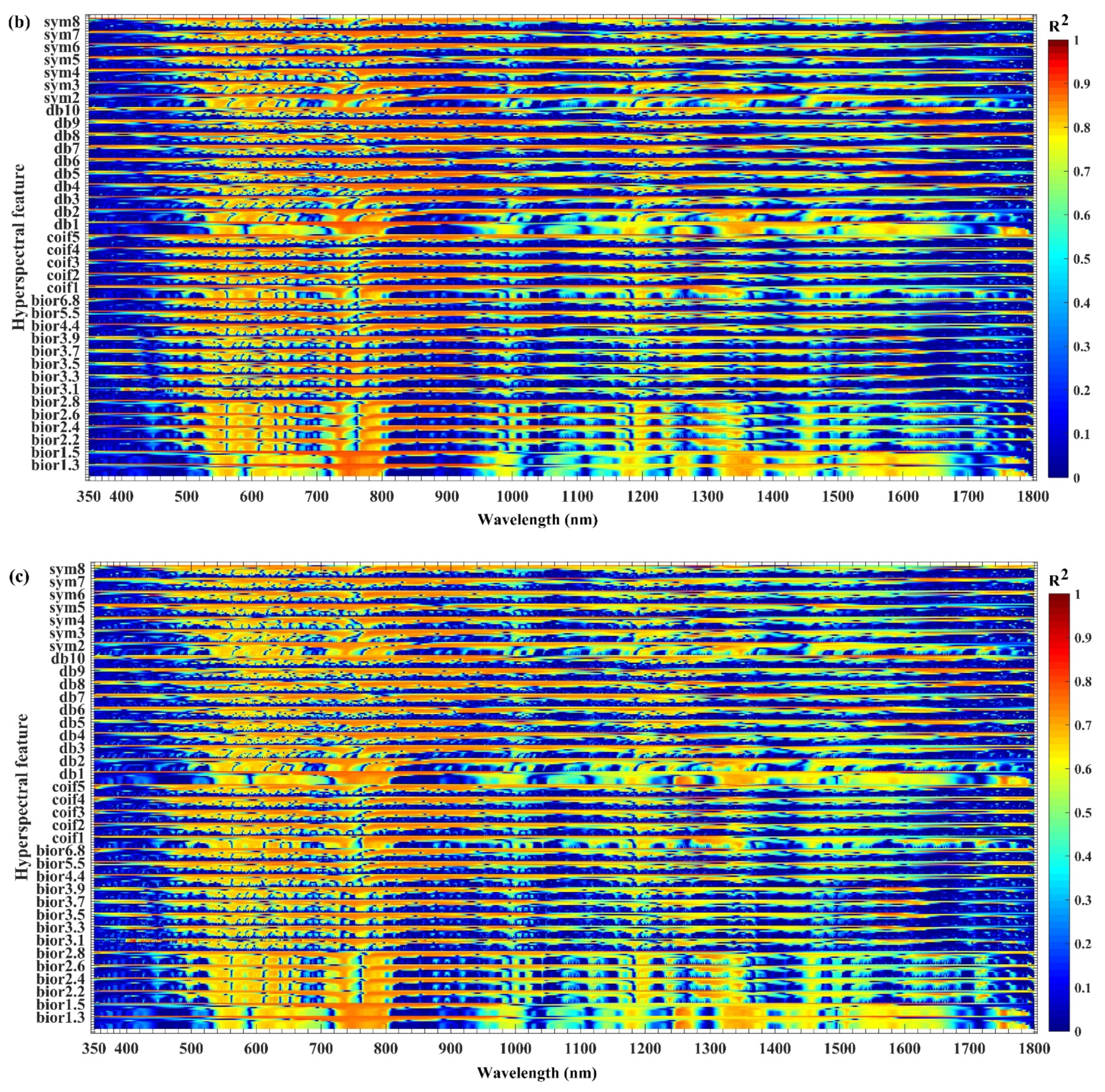
3.2. Extraction of Sensitive Hyperspectral Feature Bands
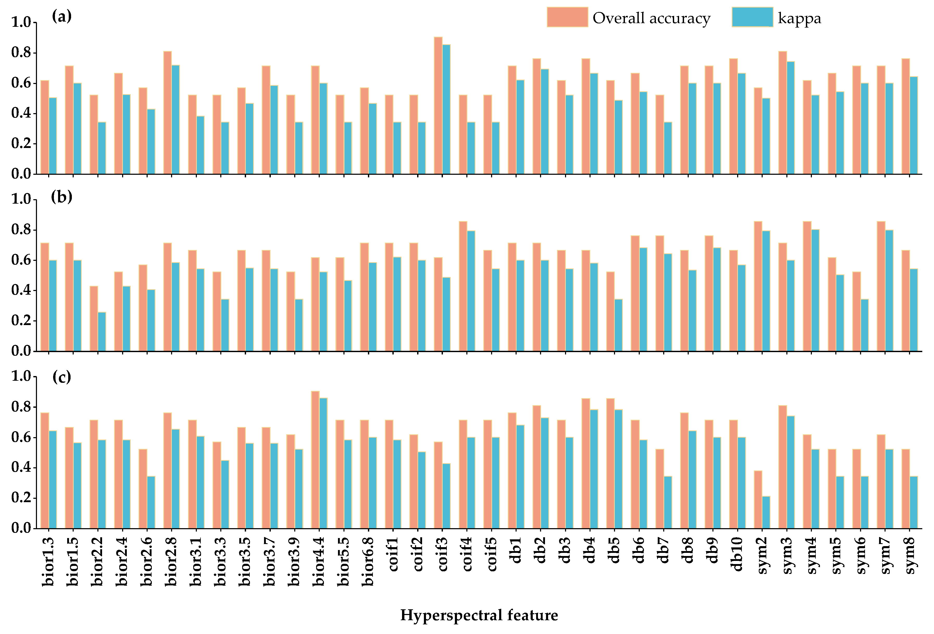
3.3. Model Results
4. Discussion
4.1. Sensitive Hyperspectral Feature Bands
4.2. Future Trends and Prospects of Remote Sensing Monitoring of JLI Outbreak
5. Conclusions
Author Contributions
Funding
Institutional Review Board Statement
Informed Consent Statement
Data Availability Statement
Conflicts of Interest
References
- Huang, X.J.; Xie, Y.W.; Bao, Y.H.; Bao, G.; Qing, S.; Bao, Y.L. Estimation of Leaf Loss Rate in Larch Infested with Erannis Jacobsoni Djak Based on Differential Spectral Continuous Wavelet Coefficient. Spectrosc. Spect. Anal. 2019, 39, 2732–2738. [Google Scholar] [CrossRef]
- Lindenmayer, D.B.; Possingham, H.P. Ranking conservation and timber management options for leadbeater’s possum in southeastern Australia using population viability analysis. Conserv. Biol. 1996, 10, 235–251. [Google Scholar] [CrossRef]
- Potapov, P.; Hansen, M.C.; Laestadius, L.; Turubanova, S.; Yaroshenko, A.; Thies, C.; Smith, W.; Zhuravleva, I.; Komarova, A.; Minnemeyer, S.; et al. The last frontiers of wilderness: Tracking loss of intact forest landscapes from 2000 to 2013. Sci. Adv. 2017, 3, e1600821. [Google Scholar] [CrossRef] [PubMed] [Green Version]
- Junttila, S.; Holopainen, M.; Vastaranta, M.; Lyytikainen-Saarenmaa, P.; Kaartinen, H.; Hyyppa, J.; Hyyppa, H. The potential of dual-wavelength terrestrial lidar in early detection of Ips typographus (L.) infestation—Leaf water content as a proxy. Remote Sens. Environ. 2019, 231, 111264. [Google Scholar] [CrossRef]
- Karvemo, S.; Johansson, V.; Schroeder, M.; Ranius, T. Local colonization-extinction dynamics of a tree-killing bark beetle during a large-scale outbreak. Ecosphere 2016, 7, e01257. [Google Scholar] [CrossRef] [Green Version]
- Huo, L.N.; Persson, H.J.; Lindberg, E. Early detection of forest stress from European spruce bark beetle attack, and a new vegetation index: Normalized distance red & SWIR (NDRS). Remote Sens. Environ. 2021, 255, 112240. [Google Scholar] [CrossRef]
- Foster, A.C.; Walter, J.A.; Shugart, H.H.; Sibold, J.; Negron, J. Spectral evidence of early-stage spruce beetle infestation in Engelmann spruce. For. Ecol. Manag. 2017, 384, 347–357. [Google Scholar] [CrossRef] [Green Version]
- Niemann, K.O.; Quinn, G.; Stephen, R.; Visintini, F.; Parton, D. Hyperspectral Remote Sensing of Mountain Pine Beetle with an Emphasis on Previsual Assessment. Can. J. Remote Sens. 2015, 41, 191–202. [Google Scholar] [CrossRef]
- Cheng, T.; Riaño, D.; Ustin, S.L. Detecting diurnal and seasonal variation in canopy water content of nut tree orchards from airborne imaging spectroscopy data using continuous wavelet analysis. Remote Sens. Environ. 2014, 143, 39–53. [Google Scholar] [CrossRef]
- Xi, G.L.; Huang, X.J.; Bao, Y.H.; Bao, G.; Tong, S.Q.; Dashzebegd, G.; Nanzadd, T.; Dorjsurene, A.; Davaadorj, E.; Ariunaad, M. Hyperspectral Discrimination of Different Canopy Colors in Erannis Jacobsoni Djak-Infested Larch. Spectrosc. Spect. Anal. 2020, 40, 2925–2931. [Google Scholar] [CrossRef]
- Ortiz, S.M.; Breidenbach, J.; Kändler, G. Early Detection of Bark Beetle Green Attack Using TerraSAR-X and RapidEye Data. Remote Sens. 2013, 5, 1912–1931. [Google Scholar] [CrossRef] [Green Version]
- Wulder, M.A.; White, J.C.; Bentz, B.; Alvarez, M.F.; Coops, N.C. Estimating the probability of mountain pine beetle red-attack damage. Remote Sens. Environ. 2006, 101, 150–166. [Google Scholar] [CrossRef]
- Tane, Z.; Roberts, D.; Koltunov, A.; Sweeney, S.; Ramirez, C. A framework for detecting conifer mortality across an ecoregion using high spatial resolution spaceborne imaging spectroscopy. Remote Sens. Environ. 2018, 209, 195–210. [Google Scholar] [CrossRef]
- Meddens, A.J.H.; Hicke, J.A.; Vierling, L.A.; Hudak, A.T. Evaluating methods to detect bark beetle-caused tree mortality using single-date and multi-date Landsat imagery. Remote Sens. Environ. 2013, 132, 49–58. [Google Scholar] [CrossRef]
- Meddens, A.J.H.; Hicke, J.A.; Vierling, L.A. Evaluating the potential of multispectral imagery to map multiple stages of tree mortality. Remote Sens. Environ. 2011, 115, 1632–1642. [Google Scholar] [CrossRef]
- Wulder, M.A.; Dymond, C.C.; White, J.C.; Leckie, D.G.; Carroll, A.L. Surveying mountain pine beetle damage of forests: A review of remote sensing opportunities. For. Ecol. Manag. 2006, 221, 27–41. [Google Scholar] [CrossRef]
- Wulder, M.A.; White, J.C.; Carroll, A.L.; Coops, N.C. Challenges for the operational detection of mountain pine beetle green attack with remote sensing. For. Chron. 2009, 85, 32–38. [Google Scholar] [CrossRef] [Green Version]
- Pu, R.; Ge, S.; Kelly, N.M.; Gong, P. Spectral absorption features as indicators of water status in coast live oak (Quercus agrifolia) leaves. Int. J. Remote Sens. 2003, 24, 1799–1810. [Google Scholar] [CrossRef]
- Zhang, J.Y.; Sun, H.; Gao, D.H.; Qiao, L.; Liu, N.; Li, M.Z.; Zhang, Y. Detection of Canopy Chlorophyll Content of Corn Based on Continuous Wavelet Transform Analysis. Remote Sens. 2020, 12, 2741. [Google Scholar] [CrossRef]
- Asner, G.P.; Martin, R.E.; Keith, L.M.; Heller, W.P.; Hughes, M.A.; Vaughn, N.R.; Hughes, R.F.; Balzotti, C. A Spectral Mapping Signature for the Rapid Ohia Death (ROD) Pathogen in Hawaiian Forests. Remote Sens. 2018, 10, 404. [Google Scholar] [CrossRef] [Green Version]
- Huang, L.S.; Wu, K.; Huang, W.J.; Dong, Y.Y.; Ma, H.Q.; Liu, Y.; Liu, L.Y. Detection of Fusarium Head Blight in Wheat Ears Using Continuous Wavelet Analysis and PSO-SVM. Agriculture 2021, 11, 998. [Google Scholar] [CrossRef]
- Omeer, A.A.; Deshmukh, R.R. Improving the classification of invasive plant species by using continuous wavelet analysis and feature reduction techniques. Ecol. Inform. 2021, 61, 101181. [Google Scholar] [CrossRef]
- Cheng, T.; Rivard, B.; Sanchez-Azofeifa, G.A.; Feng, J.; Calvo-Polanco, M. Continuous wavelet analysis for the detection of green attack damage due to mountain pine beetle infestation. Remote Sens. Environ. 2010, 114, 899–910. [Google Scholar] [CrossRef]
- Jia, M.; Li, D.; Colombo, R.; Wang, Y.; Wang, X.; Cheng, T.; Zhu, Y.; Yao, X.; Xu, C.J.; Ouer, G.; et al. Quantifying Chlorophyll Fluorescence Parameters from Hyperspectral Reflectance at the Leaf Scale under Various Nitrogen Treatment Regimes in Winter Wheat. Remote Sens. 2019, 11, 2838. [Google Scholar] [CrossRef] [Green Version]
- He, R.Y.; Li, H.; Qiao, X.J.; Jiang, J.B. Using wavelet analysis of hyperspectral remote-sensing data to estimate canopy chlorophyll content of winter wheat under stripe rust stress. Int. J. Remote Sens. 2018, 39, 4059–4076. [Google Scholar] [CrossRef]
- Cheng, T.; Rivard, B.; Sanchez-Azofeifa, A. Spectroscopic determination of leaf water content using continuous wavelet analysis. Remote Sens. Environ. 2011, 115, 659–670. [Google Scholar] [CrossRef]
- Pepke, S.; Wold, B.; Mortazavi, A. Computation for ChIP-seq and RNA-seq studies. Nat. Methods 2009, 6, S22–S32. [Google Scholar] [CrossRef]
- Zhang, N.; Zhang, X.L.; Yang, G.J.; Zhu, C.H.; Huo, L.N.; Feng, H.K. Assessment of defoliation during the Dendrolimus tabulaeformis Tsai et Liu disaster outbreak using UAV-based hyperspectral images. Remote Sens. Environ. 2018, 217, 323–339. [Google Scholar] [CrossRef]
- Tian, L.; Xue, B.W.; Wang, Z.Y.; Li, D.; Yao, X.; Cao, Q.; Zhu, Y.; Cao, W.X.; Cheng, T. Spectroscopic detection of rice leaf blast infection from asymptomatic to mild stages with integrated machine learning and feature selection. Remote Sens. Environ. 2021, 257, 112350. [Google Scholar] [CrossRef]
- Sarangdhar, A.A.; Pawar, V.R. Machine Learning Regression Technique for Cotton Leaf Disease Detection and Controlling using IoT. In Proceedings of the 2017 International Conference of Electronics, Communication and Aerospace Technology (Iceca), Coimbatore, India, 20–22 April 2017; Volume 2, pp. 449–454. [Google Scholar]
- Ulziibaatar, M.; Matsui, K. Herders’ Perceptions about Rangeland Degradation and Herd Management: A Case among Traditional and Non-Traditional Herders in Khentii Province of Mongolia. Sustainability 2021, 13, 7896. [Google Scholar] [CrossRef]
- Ishimaru, Y.; Kim, S.; Tsukamoto, T.; Oki, H.; Kobayashi, T.; Watanabe, S.; Matsuhashi, S.; Takahashi, M.; Nakanishi, H.; Mori, S.; et al. Mutational reconstructed ferric chelate reductase confers enhanced tolerance in rice to iron deficiency in calcareous soil. Proc. Natl. Acad. Sci. USA 2007, 104, 7373–7378. [Google Scholar] [CrossRef] [Green Version]
- Wang, Q.; Xue, J.; Chen, J.-L.; Fan, Y.-H.; Zhang, G.-Q.; Xie, R.-Z.; Ming, B.; Hou, P.; Wang, K.-R.; Li, S.-K. Key indicators affecting maize stalk lodging resistance of different growth periods under different sowing dates. J. Integr. Agric. 2020, 19, 2419–2428. [Google Scholar] [CrossRef]
- Bayer, A. Fertilizer Rate and Substrate Water Content Effect on Growth and Flowering of Beardtongue. Horticulturae 2020, 6, 57. [Google Scholar] [CrossRef]
- Bashir, T.; Naz, S.; Bano, A. Plant Growth Promoting Rhizobacteria in Combination with Plant Growth Regulators Attenuate the Effect of Drought Stress. Pak. J. Bot 2020, 52, 783–792. [Google Scholar] [CrossRef]
- Bean, E.Z.; Huffaker, R.G.; Migliaccio, K.W. Estimating Field Capacity from Volumetric Soil Water Content Time Series Using Automated Processing Algorithms. Vadose Zone J. 2018, 17, 1–12. [Google Scholar] [CrossRef] [Green Version]
- Boeva, V.; Lermine, A.; Barette, C.; Guillouf, C.; Barillot, E. Nebula--a web-server for advanced ChIP-seq data analysis. Bioinformatics 2012, 28, 2517–2519. [Google Scholar] [CrossRef] [Green Version]
- Malone, B.M.; Tan, F.; Bridges, S.M.; Peng, Z. Comparison of four ChIP-Seq analytical algorithms using rice endosperm H3K27 trimethylation profiling data. PLoS ONE 2011, 6, e25260. [Google Scholar] [CrossRef] [PubMed]
- Wang, J.J.; Wang, T.J.; Skidmore, A.K.; Shi, T.Z.; Wu, G.F. Evaluating Different Methods for Grass Nutrient Estimation from Canopy Hyperspectral Reflectance. Remote Sens. 2015, 7, 5901–5917. [Google Scholar] [CrossRef] [Green Version]
- Yang, J.; Sun, L.; Xing, W.; Feng, G.; Bai, H.; Wang, J. Hyperspectral prediction of sugarbeet seed germination based on gauss kernel SVM. Spectrochim. Acta A Mol. Biomol. Spectrosc. 2021, 253, 119585. [Google Scholar] [CrossRef]
- Zhang, T.; Huang, Y.B.; Reddy, K.N.; Yang, P.T.; Zhao, X.H.; Zhang, J.C. Using Machine Learning and Hyperspectral Images to Assess Damages to Corn Plant Caused by Glyphosate and to Evaluate Recoverability. Agronomy 2021, 11, 583. [Google Scholar] [CrossRef]
- Sun, H.; Feng, M.; Xiao, L.; Yang, W.; Ding, G.; Wang, C.; Jia, X.; Wu, G.; Zhang, S. Potential of Multivariate Statistical Technique Based on the Effective Spectra Bands to Estimate the Plant Water Content of Wheat Under Different Irrigation Regimes. Front. Plant Sci. 2021, 12, 631573. [Google Scholar] [CrossRef]
- Yu, R.; Ren, L.L.; Luo, Y.Q. Early detection of pine wilt disease in Pinus tabuliformis in North China using a field portable spectrometer and UAV-based hyperspectral imagery. For. Ecosyst. 2021, 8, 1–19. [Google Scholar] [CrossRef]
- De Almeida, C.T.; Galvão, L.S.; de Oliveira Cruz e Aragão, L.E.; Ometto, J.P.H.B.; Jacon, A.D.; de Souza Pereira, F.R.; Sato, L.Y.; Lopes, A.P.; de Alencastro Graça, P.M.; de Jesus Silva, C.V.; et al. Combining LiDAR and hyperspectral data for aboveground biomass modeling in the Brazilian Amazon using different regression algorithms. Remote Sens. Environ. 2019, 232, 111323. [Google Scholar] [CrossRef]
- Immitzer, M.; Bock, S.; Einzmann, K.; Vuolo, F.; Pinnel, N.; Wallner, A.; Atzberger, C. Fractional cover mapping of spruce and pine at 1 ha resolution combining very high and medium spatial resolution satellite imagery. Remote Sens. Environ. 2018, 204, 690–703. [Google Scholar] [CrossRef] [Green Version]
- Fassnacht, F.E.; Latifi, H.; Ghosh, A.; Joshi, P.K.; Koch, B. Assessing the potential of hyperspectral imagery to map bark beetle-induced tree mortality. Remote Sens. Environ. 2014, 140, 533–548. [Google Scholar] [CrossRef]
- Wietecha, M.; Jelowicki, L.; Mitelsztedt, K.; Miscicki, S.; Sterenczak, K. The capability of species-related forest stand characteristics determination with the use of hyperspectral data. Remote Sens. Environ. 2019, 231, 111232. [Google Scholar] [CrossRef]
- Suess, S.; van der Linden, S.; Okujeni, A.; Griffiths, P.; Leitao, P.J.; Schwieder, M.; Hostert, P. Characterizing 32 years of shrub cover dynamics in southern Portugal using annual Landsat composites and machine learning regression modeling. Remote Sens. Environ. 2018, 219, 353–364. [Google Scholar] [CrossRef]
- Hart, S.J.; Veblen, T.T. Detection of spruce beetle-induced tree mortality using high- and medium-resolution remotely sensed imagery. Remote Sens. Environ. 2015, 168, 134–145. [Google Scholar] [CrossRef] [Green Version]
- Grass, I.; Kubitza, C.; Krishna, V.V.; Corre, M.D.; Musshoff, O.; Putz, P.; Drescher, J.; Rembold, K.; Ariyanti, E.S.; Barnes, A.D.; et al. Trade-offs between multifunctionality and profit in tropical smallholder landscapes. Nat. Commun. 2020, 11, 1186. [Google Scholar] [CrossRef] [PubMed] [Green Version]
- Ballhorn, U.; Siegert, F.; Mason, M.; Limin, S. Derivation of burn scar depths and estimation of carbon emissions with LIDAR in Indonesian peatlands. Proc. Natl. Acad. Sci. USA 2009, 106, 21213–21218. [Google Scholar] [CrossRef] [Green Version]
- Zarco-Tejada, P.J.; Hornero, A.; Beck, P.S.A.; Kattenborn, T.; Kempeneers, P.; Hernandez-Clemente, R. Chlorophyll content estimation in an open-canopy conifer forest with Sentinel-2A and hyperspectral imagery in the context of forest decline. Remote Sens. Environ. 2019, 223, 320–335. [Google Scholar] [CrossRef] [PubMed]
- Liu, N.; Xing, Z.Z.; Zhao, R.M.; Qiao, L.; Li, M.Z.; Liu, G.; Sun, H. Analysis of Chlorophyll Concentration in Potato Crop by Coupling Continuous Wavelet Transform and Spectral Variable Optimization. Remote Sens. 2020, 12, 2826. [Google Scholar] [CrossRef]
- An, G.Q.; Xing, M.F.; Liao, C.H.; He, B.B. Estimating Chlorophyll Content of Rice Based on Uav-Based Hyperspectral Imagery and Continuous Wavelet Transform. In Proceedings of the Igarss 2020-2020 Ieee International Geoscience and Remote Sensing Symposium, Waikoloa, HI, USA, 26 September–2 October 2020; pp. 5270–5273. [Google Scholar] [CrossRef]
- Chen, S.M.; Hu, T.T.; Luo, L.H.; He, Q.; Zhang, S.W.; Li, M.Y.; Cui, X.L.; Li, H.X. Rapid estimation of leaf nitrogen content in apple-trees based on canopy hyperspectral reflectance using multivariate methods. Infrared Phys. Technol. 2020, 111, 103542. [Google Scholar] [CrossRef]
- Gu, Q.; Sheng, L.; Zhang, T.H.; Lu, Y.W.; Zhang, Z.J.; Zheng, K.F.; Hu, H.; Zhou, H.K. Early detection of tomato spotted wilt virus infection in tobacco using the hyperspectral imaging technique and machine learning algorithms. Comput. Electron. Agric. 2019, 167, 105066. [Google Scholar] [CrossRef]
- Gao, Z.M.; Zhao, Y.R.; Khot, L.R.; Hoheisel, G.A.; Zhang, Q. Optical sensing for early spring freeze related blueberry bud damage detection: Hyperspectral imaging for salient spectral wavelengths identification. Comput. Electron. Agric. 2019, 167, 105025. [Google Scholar] [CrossRef]


| Tree Class | Healthy Tree | Damaged Early Tree | Damaged Tree |
|---|---|---|---|
| Leaf loss rate | 0–5% | 5–15% | 15–100% |
| Canopy color | Green | Green | Yellow, red, and gray |
| Chlorophyll Content (μg/cm2) | Fresh Weight Moisture Content | Dry Weight Moisture Content | ||||||||||
|---|---|---|---|---|---|---|---|---|---|---|---|---|
| Max | Min | Mean | Std | Max | Min | Mean | Std | Max | Min | Mean | Std | |
| Healthy tree | 50.30 | 39.39 | 44.51 | 2.79 | 0.74 | 0.62 | 0.69 | 0.04 | 2.76 | 1.61 | 2.00 | 0.37 |
| Damaged early tree | 38.45 | 28.41 | 32.87 | 3.35 | 0.67 | 0.57 | 0.62 | 0.04 | 1.54 | 1.09 | 1.31 | 0.15 |
| Damaged tree | 27.16 | 4.41 | 13.95 | 5.38 | 0.57 | 0.02 | 0.26 | 0.15 | 1.08 | 0.02 | 0.40 | 0.28 |
| Classes | Healthy | Damaged Early | Damaged | Total | UA |
|---|---|---|---|---|---|
| OA: 90.47%, Kappa: 85.42% | |||||
| Healthy | 4 | 0 | 0 | 4 | 100% |
| Damaged Early | 1 | 4 | 0 | 5 | 80% |
| Damaged | 0 | 1 | 11 | 12 | 91.68% |
| Total | 5 | 5 | 11 | 21 | |
| PA | 80% | 80% | 100% | 90.48% | |
| Classes | Healthy | Damaged Early | Damaged | Total | UA |
|---|---|---|---|---|---|
| OA: 85.71%, Kappa: 79.48% | |||||
| Healthy | 5 | 1 | 0 | 6 | 83.33% |
| Damaged Early | 0 | 4 | 2 | 6 | 66.68% |
| Damaged | 0 | 0 | 9 | 9 | 100% |
| Total | 5 | 5 | 11 | 21 | |
| PA | 100% | 80% | 81.82% | 85.71% | |
| Classes | Healthy | Damaged Early | Damaged | Total | UA |
|---|---|---|---|---|---|
| OA: 90.48%, Kappa: 86% | |||||
| Healthy | 4 | 0 | 0 | 4 | 100% |
| Damaged Early | 1 | 5 | 1 | 6 | 71.43% |
| Damaged | 0 | 0 | 10 | 10 | 100% |
| Total | 5 | 5 | 11 | 21 | |
| PA | 80% | 100% | 90.91% | 90.48% | |
| Biochemical Component | Main Sensitive Band Range (nm) | Sensitive Band Etracted by Findpeaks–SPA (nm) |
|---|---|---|
| Chlorophyll content | 540–581, 596–699, 723–804, 954–956, 974–1011, 1134–1143, 1166–1199, 1245–1275, 1313–1386, 1412–1467, 1483–1485, 1500–1664, 1743–1770, 1784–1785 | 450, 644, 1042(coif3) |
| Fresh weight moisture content | 537–583, 595–709, 723–804, 953–962, 967–1010, 1053–1083, 1130–1139, 1162–1206, 1247–1279, 1315–1386, 1404–1468, 1480–1486, 1503–1672, 1746–1772, 1783–1785 | 446, 563, 1221, 1620, 1362, 1711(coif4) |
| Dry weight moisture content | 542–579, 598–679, 723–803, 978–1007, 1168–1195, 1245–1274, 1316–1386, 1416–1426, 1439–1465, 1503–1519, 1533–1654, 1744–1769, 1784–1785 | 382, 734, 951(bior4.4) |
Publisher’s Note: MDPI stays neutral with regard to jurisdictional claims in published maps and institutional affiliations. |
© 2021 by the authors. Licensee MDPI, Basel, Switzerland. This article is an open access article distributed under the terms and conditions of the Creative Commons Attribution (CC BY) license (https://creativecommons.org/licenses/by/4.0/).
Share and Cite
Xi, G.; Huang, X.; Xie, Y.; Gang, B.; Bao, Y.; Dashzebeg, G.; Nanzad, T.; Dorjsuren, A.; Enkhnasan, D.; Ariunaa, M. Detection of Larch Forest Stress from Jas’s Larch Inchworm (Erannis jacobsoni Djak) Attack Using Hyperspectral Remote Sensing. Remote Sens. 2022, 14, 124. https://doi.org/10.3390/rs14010124
Xi G, Huang X, Xie Y, Gang B, Bao Y, Dashzebeg G, Nanzad T, Dorjsuren A, Enkhnasan D, Ariunaa M. Detection of Larch Forest Stress from Jas’s Larch Inchworm (Erannis jacobsoni Djak) Attack Using Hyperspectral Remote Sensing. Remote Sensing. 2022; 14(1):124. https://doi.org/10.3390/rs14010124
Chicago/Turabian StyleXi, Guilin, Xiaojun Huang, Yaowen Xie, Bao Gang, Yuhai Bao, Ganbat Dashzebeg, Tsagaantsooj Nanzad, Altanchimeg Dorjsuren, Davaadorj Enkhnasan, and Mungunkhuyag Ariunaa. 2022. "Detection of Larch Forest Stress from Jas’s Larch Inchworm (Erannis jacobsoni Djak) Attack Using Hyperspectral Remote Sensing" Remote Sensing 14, no. 1: 124. https://doi.org/10.3390/rs14010124