
A Random Forest Algorithm for Retrieving Canopy Chlorophyll Content of Wheat and Soybean Trained with PROSAIL Simulations Using Adjusted Average Leaf Angle

 ,
,  ,
,  ,
,  , ,
, ,
Abstract
:
1. Introduction
2. Data and Methods
2.1. Experimental Areas and Ground Data
2.1.1. Wheat Experimental Area
2.1.2. Soybean Experimental Area
2.1.3. Ground Data
- (1)
- Determination of canopy chlorophyll content
- (2)
- Canopy reflectance measurements
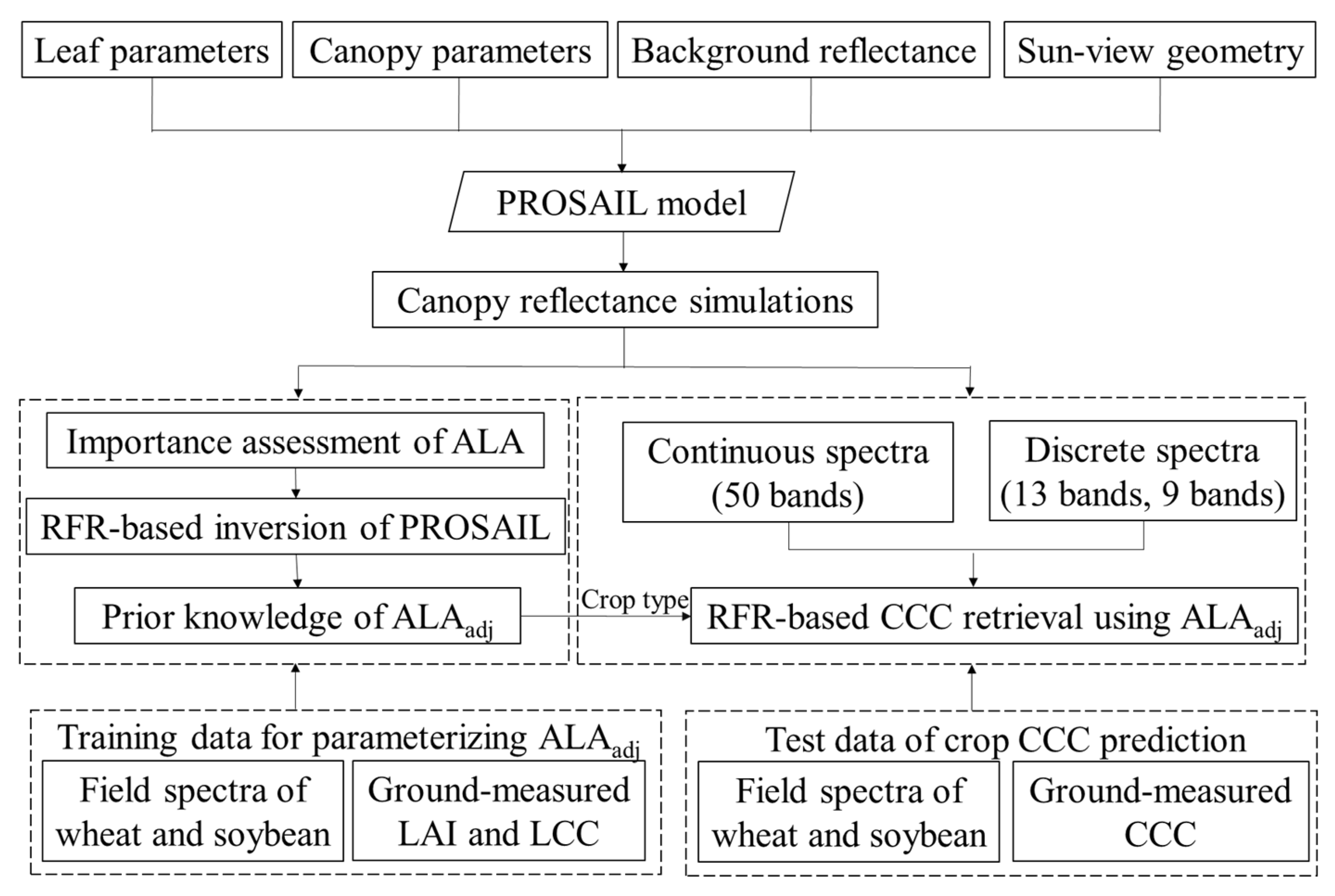
2.2. Spectra Simulation
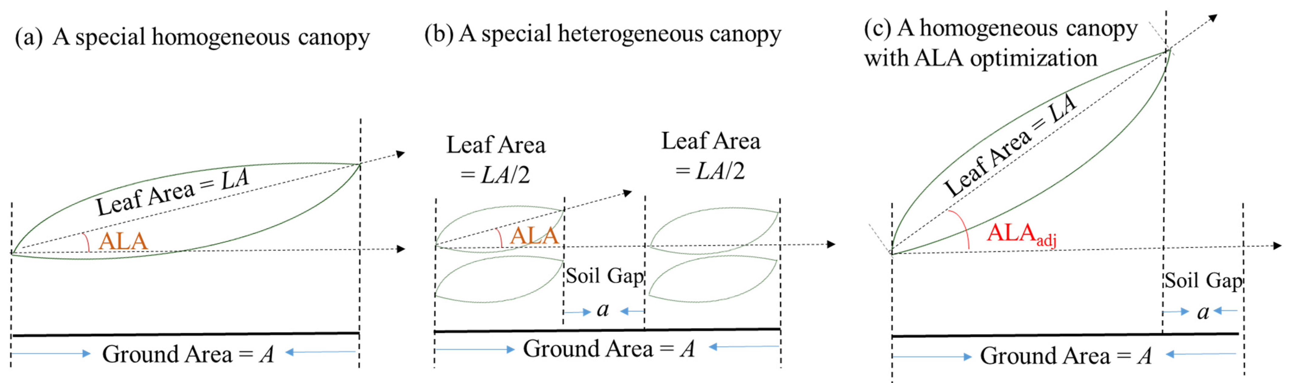
2.2.1. Spectra Simulation of Homogeneous Canopy Based on PROSAIL Model
2.2.2. Spectra Simulation of the Heterogeneous Canopy with Mixed Pixels
2.3. Methods
2.3.1. Random Forest
2.3.2. Importance Assessment Method of Vegetation Variables on Canopy Reflectance
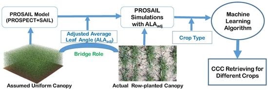
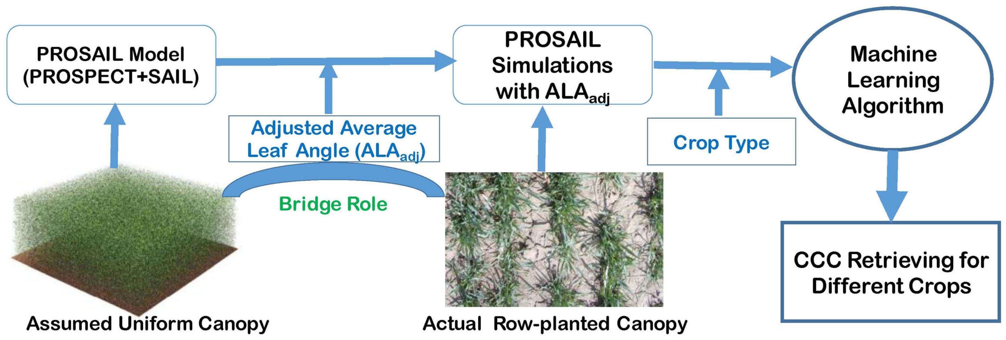
2.3.3. PROSAIL Parameterization Scheme of ALAadj Based on Measured Spectrum and Non-ALA Parameters
2.3.4. CCC Retrieval Model, Based on ALAadj Related to Crop Types
2.3.5. Validation Method
3. Results and Analysis
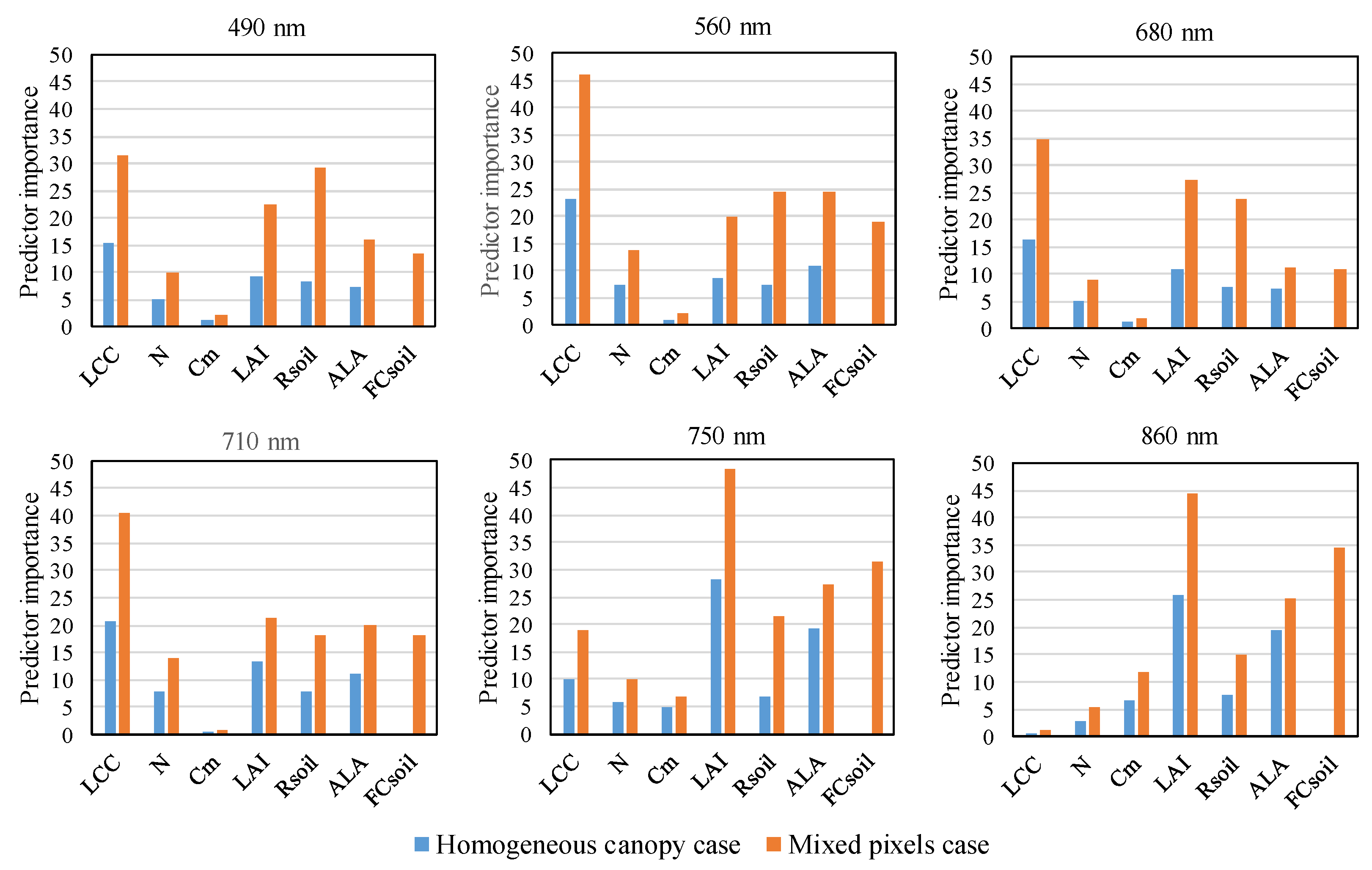
3.1. Influences of Vegetation Variables on Canopy Reflectance
3.2. ALAadj Parameterization of the PROSAIL Model for Wheat and Soybean
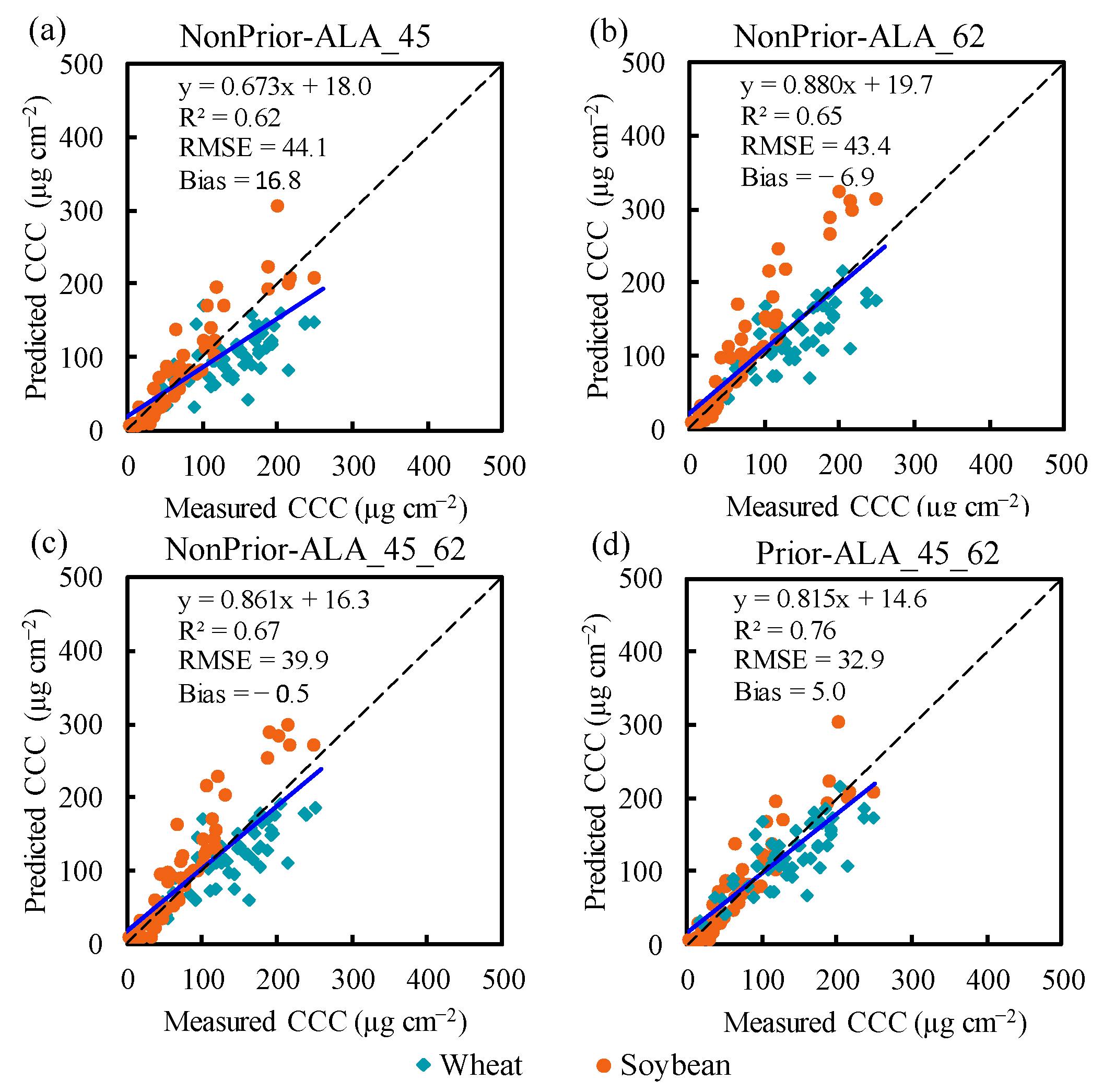
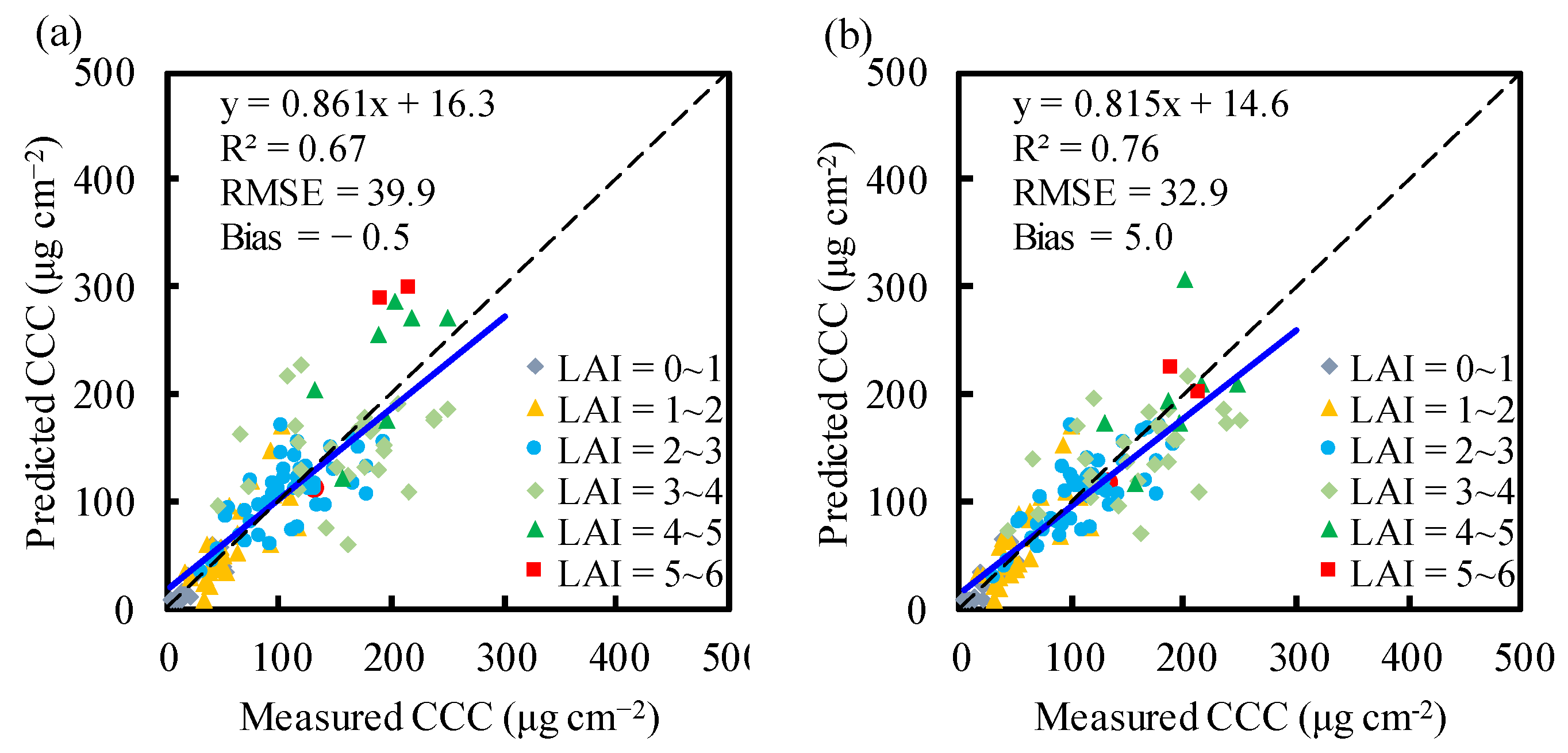
3.3. CCC Retrieval with Prior ALAadj Knowledge for Wheat and Soybean
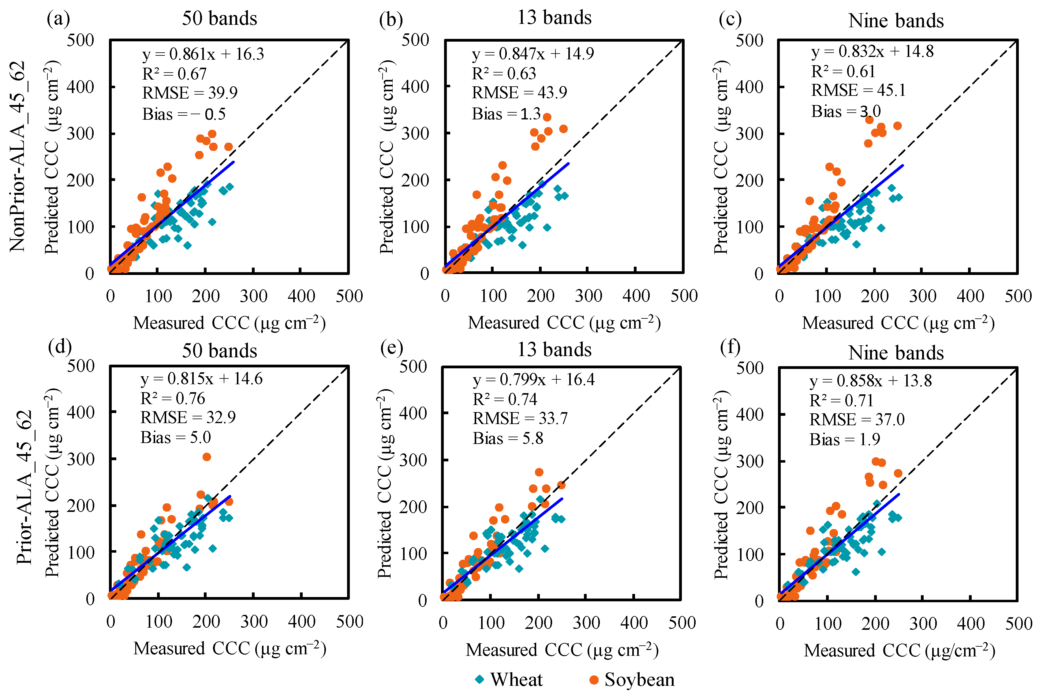
3.4. Performance Comparison of the Improved CCC Retrieval Model Using Continuous and Discrete Spectra
4. Discussion
4.1. Contribution of Our Proposed Method to PROSAIL-Based Retrieval of Crop Parameters
4.2. Reliability and Limitation of the ALAadj Parameterization Associated with Crop Types
4.3. Prospects of Our Proposed Method of Crop CCC Estimation Based on Satellite Data
5. Conclusions
Supplementary Materials
Author Contributions
Funding
Institutional Review Board Statement
Informed Consent Statement
Acknowledgments
Conflicts of Interest
References
- Ustin, S.L.; Gitelson, A.A.; Jacquemoud, S.; Schaepman, M.; Asner, G.P.; Gamon, J.A.; Zarco-Tejada, P.J. Retrieval of foliar information about plant pigment systems from high resolution spectroscopy. Remote Sens. Environ. 2019, 113, S67–S77. [Google Scholar] [CrossRef] [Green Version]
- Croft, H.; Chen, J.M.; Zhang, Y. The applicability of empirical vegetation indices for determining leaf chlorophyll content over different leaf and canopy structures. Ecol. Complex. 2014, 17, 119–130. [Google Scholar] [CrossRef]
- Croft, H.; Chen, J.M.; Luo, X.; Bartlett, P.; Chen, B.; Staebler, R.M. Leaf chlorophyll content as a proxy for leaf photosynthetic capacity. Glob. Chang. Biol. 2017, 23, 3513–3524. [Google Scholar] [CrossRef]
- He, R.; Li, H.; Qiao, X.; Jiang, J. Using wavelet analysis of hyperspectral remote-sensing data to estimate canopy chlorophyll content of winter wheat under stripe rust stress. Int. J. Remote Sens. 2018, 39, 4059–4076. [Google Scholar] [CrossRef]
- Gitelson, A.A.; Viña, A.; Verma, S.B.; Rundquist, D.C.; Arkebauer, T.J.; Keydan, G.; Leavitt, B.; Ciganda, V.; Burba, G.G.; Suyker, A.E. Relationship between gross primary production and chlorophyll content in crops: Implications for the synoptic monitoring of vegetation productivity. J. Geophys. Res. Atmos. 2006, 111. [Google Scholar] [CrossRef] [Green Version]
- Gitelson, A.A.; Peng, Y.; Arkebauer, T.J.; Schepers, J. Relationships between gross primary production, green LAI, and canopy chlorophyll content in maize: Implications for remote sensing of primary production. Remote Sens. Environ. 2014, 144, 65–72. [Google Scholar] [CrossRef]
- Porra, R.J. The chequered history of the development and use of simultaneous equations for the accurate determination of chlorophylls a and b. Photosynth. Res. 2002, 73, 149–156. [Google Scholar] [CrossRef]
- Cerovic, Z.G.; Masdoumier, G.; Ghozlen, N.B.; Latouche, G. A new optical leaf-clip meter for simultaneous non-destructive assessment of leaf chlorophyll and epidermal flavonoids. Physiol. Plant. 2012, 146, 251–260. [Google Scholar] [CrossRef]
- Pinar, A.; Curran, P.J. Grass chlorophyll and the reflflectance red edge. Int. J. Remote Sens. 1996, 17, 351–357. [Google Scholar] [CrossRef]
- Maccioni, A.; Agati, G.; Mazzinghi, P. New vegetation indices for remote measurement of chlorophylls based on leaf directional reflectance spectra. J. Photochem. Photobiol. B Biol. 2001, 61, 52–61. [Google Scholar] [CrossRef]
- Gitelson, A.A.; Gritz, Y.; Merzlyak, M.N. Relationships between leaf chlorophyll content and spectral reflectance and algorithms for non-destructive chlorophyll assessment in higher plant leaves. J. Plant. Physiol. 2003, 160, 271–282. [Google Scholar] [CrossRef]
- Cui, S.; Zhou, K. A comparison of the predictive potential of various vegetation indices for leaf chlorophyll content. Earth Sci. Inform. 2017, 10, 169–181. [Google Scholar] [CrossRef]
- Peng, Y.; Anthony, N.R.; Timothy, A.; Gitelson, A.A. Assessment of canopy chlorophyll content retrieval in maize and soybean: Implications of hysteresis on the development of generic algorithms. Remote Sens. 2017, 9, 226. [Google Scholar] [CrossRef] [Green Version]
- Dash, J.; Curran, P.J. The MERIS terrestrial chlorophyll index. Int. J. Remote Sens. 2004, 25, 5403–5413. [Google Scholar] [CrossRef]
- Gitelson, A.A.; Viña, A.; Ciganda, V.; Rundquist, D.C.; Arkebauer, T.J. Remote estimation of canopy chlorophyll content in crops. Geophys. Res. Lett. 2005, 32, 1–4. [Google Scholar] [CrossRef] [Green Version]
- Durbha, S.S.; King, R.L.; Younan, N.H. Support vector machines regression for retrieval of leaf area index from multiangle imaging spectroradiometer. Remote Sens. Environ. 2007, 107, 348–361. [Google Scholar] [CrossRef]
- Feilhauer, H.; Asner, G.P.; Martin, R.E. Multi-method ensemble selection of spectral bands related to leaf biochemistry. Remote Sens. Environ. 2015, 164, 57–65. [Google Scholar] [CrossRef]
- Shah, S.H.; Angel, Y.; Houborg, R.; Ali, S.; McCabe, M.F. A Random Forest Machine Learning Approach for the Retrieval of Leaf Chlorophyll Content in Wheat. Remote Sens. 2019, 11, 920. [Google Scholar] [CrossRef] [Green Version]
- Danner, M.; Berger, K.; Wocher, M.; Mauser, W.; Hank, T. Efficient RTM-based training of machine learning regression algorithms to quantify biophysical & biochemical traits of agricultural crops. ISPRS J. Photogramm. Remote Sens. 2021, 173, 278–296. [Google Scholar] [CrossRef]
- Boateng, E.Y.; Otoo, J.; Abaye, D.A. Basic Tenets of Classification Algorithms K-Nearest-Neighbor, Support Vector Machine, Random Forest and Neural Network: A Review. J. Data Anal. Inf. Process. 2020, 8, 341–357. [Google Scholar] [CrossRef]
- Belgiu, M.; Drăgut, L. Random forest in remote sensing: A review of applications and future directions. ISPRS J. Photogramm. 2016, 114, 24–31. [Google Scholar] [CrossRef]
- Wang, L.; Zhou, X.; Zhu, X.; Dong, Z.; Guo, W. Estimation of biomass in wheat using random forest regression algorithm and remote sensing data. Crop J. 2016, 4, 212–219. [Google Scholar] [CrossRef] [Green Version]
- Verrelst, J.; Camps-Valls, G.; Muñoz-Marí, J.; Rivera, J.P.; Veroustraete, F.; Clevers, J.G.P.W.; Moreno, J. Optical remote sensing and the retrieval of terrestrial vegetation bio-geophysical properties—A review. ISPRS J. Photogramm. 2015, 108, 273–290. [Google Scholar] [CrossRef]
- Jacquemoud, S.; Baret, F. PROSPECT: A model of leaf optical properties spectra. Remote Sens. Environ. 1990, 34, 75–91. [Google Scholar] [CrossRef]
- Verhoef, W. Light scattering by leaf layers with application to canopy reflflectance modeling: The SAIL model. Remote Sens. Environ. 1984, 16, 125–141. [Google Scholar] [CrossRef] [Green Version]
- Haboudane, D.; Miller, J.R.; Tremblay, N.; Zarco-Tejada, P.J.; Dextraze, L. Integrated narrow-band vegetation indices for prediction of crop chlorophyll content for application to precision agriculture. Remote Sens. Environ. 2002, 81, 416–426. [Google Scholar] [CrossRef]
- Upreti, D.; Pignatti, S.; Pascucci, S.; Tolomio, M.; Huang, W.; Casa, R. Bayesian Calibration of the Aquacrop-OS Model for Durum Wheat by Assimilation of Canopy Cover Retrieved from VENµS Satellite Data. Remote Sens. 2020, 12, 2666. [Google Scholar] [CrossRef]
- Sá, N.C.D.; Baratchi, M.; Hauser, L.T.; Bodegom, P.V. Exploring the impact of noise on hybrid inversion of PROSAIL RTM on sentinel-2 data. Remote Sens. 2021, 13, 648. [Google Scholar]
- Verrelst, J.; Rivera, J.P.; van der Tol, C.; Magnani, F.; Mohammed, G.; Moreno, J. Global sensitivity analysis of the SCOPE model: What drives simulated canopy-leaving sun-induced fluorescence? Remote Sens. Environ. 2015, 166, 8–21. [Google Scholar] [CrossRef]
- Jacquemoud, S.; Verhoef, W.; Baret, F.; Bacour, C.; Zarco-Tejada, P.J.; Asner, G.P.; François, C.; Ustin, S.L. PROSPECT+SAIL models: A review of use for vegetation characterization. Remote Sens. Environ. 2009, 113, S56–S66. [Google Scholar] [CrossRef]
- Casa, R.; Baret, F.; Buis, S.; López-Lozano, R.; Pascucci, S.; Palombo, A.; Jones, H.G. Estimation of maize canopy properties from remote sensing by inversion of 1-D and 4-D models. Precis. Agric. 2010, 11, 319–334. [Google Scholar] [CrossRef] [Green Version]
- Berger, K.; Atzberger, C.; Danner, M.; D’Urso, G.; Mauser, W.; Vuolo, F.; Hank, T. Evaluation of the PROSAIL Model Capabilities for Future Hyperspectral Model Environments: A Review Study. Remote Sens. 2018, 10, 85. [Google Scholar] [CrossRef] [Green Version]
- Ma, X.; Wang, T.; Lu, L. A Refined Four-Stream Radiative Transfer Model for Row-Planted Crops. Remote Sens. 2020, 12, 1290. [Google Scholar] [CrossRef] [Green Version]
- Danner, M.; Berger, K.; Wocher, M.; Mauser, W.; Hank, T. Fitted PROSAIL Parameterization of Leaf Inclinations, Water Content and Brown Pigment Content for Winter Wheat and Maize Canopies. Remote Sens. 2019, 11, 1150. [Google Scholar] [CrossRef] [Green Version]
- Li, D.; Chen, J.M.; Zhang, X.; Yan, Y.; Zhu, J.; Zheng, H.; Zhou, K.; Yao, X.; Tian, Y.; Zhu, Y.; et al. Improved estimation of leaf chlorophyll content of row crops from canopy reflectance spectra through minimizing canopy structural effects and optimizing off-noon observation time. Remote Sens. Environ. 2020, 248, 111985. [Google Scholar] [CrossRef]
- Liu, L.; Wang, J.; Huang, W.; Zhao, C. Detection of leaf and canopy EWT by calculating REWT from reflflectance spectra. Int. J. Remote Sens. 2010, 31, 2681–2695. [Google Scholar] [CrossRef]
- Verma, S.B.; Dobermann, A.; Cassman, K.G.; Walters, D.T.; Knops, J.M.; Arkebauer, T.J.; Suyker, A.E.; Burba, G.; Amos, B.; Yang, H.; et al. Annual carbon dioxide exchange in irrigated and rainfed maize-based agroecosystems. Agric. For. Meteorol. 2005, 131, 77–96. [Google Scholar] [CrossRef] [Green Version]
- Cui, B.; Zhao, Q.; Huang, W.; Song, X.; Ye, H.; Zhou, X. A New Integrated Vegetation Index for the Estimation of Winter Wheat Leaf Chlorophyll Content. Remote Sens. 2019, 11, 974. [Google Scholar] [CrossRef] [Green Version]
- Viña, A.; Henebry, G.M.; Gitelson, A.A. Satellite monitoring of vegetation dynamics: Sensitivity enhancement by the wide dynamic range vegetation index. Geophys. Res. Lett. 2004, 31, 373–394. [Google Scholar] [CrossRef] [Green Version]
- Rundquist, D.; Perk, R.; Leavitt, B.; Keydan, G.; Gitelson, A. Collecting spectral data over cropland vegetation using machine-positioning versus hand-positioning of the sensor. Comput. Electron. Agric. 2004, 43, 173–178. [Google Scholar] [CrossRef] [Green Version]
- Féret, J.-B.; Gitelson, A.; Noble, S.; Jacquemoud, S. PROSPECT-D: Towards modeling leaf optical properties through a complete lifecycle. Remote Sens. Environ. 2017, 193, 204–215. [Google Scholar] [CrossRef] [Green Version]
- Verhoef, W.; Jia, L.; Xiao, Q.; Su, Z. Unifified optical-thermal four-stream radiative transfer theory for homogeneous vegetation canopies. IEEE Trans. Geosci. Remote Sens. 2007, 45, 1808–1822. [Google Scholar] [CrossRef]
- Campbell, G. Derivation of an angle density function for canopies with ellipsoidal leaf angle distributions. Agric. For. Meteorol. 1990, 49, 173–176. [Google Scholar] [CrossRef]
- Verhoef, W. Theory of Radiative Transfer Models Applied in Optical Remote Sensing of Vegetation Canopies. Ph.D. Thesis, Wageningen Agricultural University, Wageningen, The Netherlands, 1998. [Google Scholar]
- Kamiyama, C.; Oikawa, S.; Kubo, T.; Hikosaka, K. Light interception in species with different functional groups coexisting in moorland plant communities. Oecologia 2010, 164, 591–599. [Google Scholar] [CrossRef] [PubMed]
- Thomas, S.C.; Winner, W.E. A rotated ellipsoidal angle density function improves estimation of foliage inclination distributions in forest canopies. Agric. For. Meteorol. 2000, 100, 19–24. [Google Scholar] [CrossRef]
- Friedl, M.; Davis, F.; Michaelsen, J.; Moritz, M. Scaling and uncertainty in the relationship between the NDVI and land surface biophysical variables: An analysis using a scene simulation model and data from FIFE. Remote Sens. Environ. 1995, 54, 233–246. [Google Scholar] [CrossRef]
- Vuolo, F.; Neugebauer, N.; Bolognesi, S.F.; Atzberger, C.; D’Urso, G. Estimation of Leaf Area Index Using DEIMOS-1 Data: Application and Transferability of a Semi-Empirical Relationship between two Agricultural Areas. Remote Sens. 2013, 5, 1274–1291. [Google Scholar] [CrossRef] [Green Version]
- Houborg, R.; McCabe, M.F. A hybrid training approach for leaf area index estimation via Cubist and random forests machine-learning. ISPRS J. Photogramm. Remote Sens. 2018, 135, 173–188. [Google Scholar] [CrossRef]
- Breiman, L. Random Forests. Mach. Learn. 2001, 45, 5–32. [Google Scholar] [CrossRef] [Green Version]
- Mutanga, O.; Adam, E.; Cho, M.A. High density biomass estimation for wetland vegetation using WorldView-2 imagery and random forest regression algorithm. Int. J. Appl. Earth Obs. Geoinf. 2012, 18, 399–406. [Google Scholar] [CrossRef]
- Liang, L.; Qin, Z.; Zhao, S.; Di, L.; Zhang, C.; Deng, M.; Lin, H.; Zhang, L.; Wang, L.; Liu, Z. Estimating crop chlorophyll content with hyperspectral vegetation indices and the hybrid inversion method. Int. J. Remote Sens. 2016, 37, 2923–2949. [Google Scholar] [CrossRef]
- Verrelst, J.; Sabater, N.; Rivera, J.P.; Muñoz-Marí, J.; Vicent, J.; Camps-Valls, G.; Moreno, J. Emulation of Leaf, Canopy and Atmosphere Radiative Transfer Models for Fast Global Sensitivity Analysis. Remote Sens. 2016, 8, 673. [Google Scholar] [CrossRef] [Green Version]
- Weiss, M.; Baret, F.; Smith, G.; Jonckheere, I.; Coppin, P. Review of methods for in situ leaf area index (LAI) determination: Part II. Estimation of LAI, errors and sampling. Agric. For. Meteorol. 2004, 121, 37–53. [Google Scholar] [CrossRef]
- Wang, W.-M.; Li, Z.-L.; Su, H. Comparison of leaf angle distribution functions: Effects on extinction coefficient and fraction of sunlit foliage. Agric. For. Meteorol. 2007, 143, 106–122. [Google Scholar] [CrossRef]
- Kimes, D.; Knyazikhin, Y.; Privette, J.; Abuelgasim, A.; Gao, F. Inversion methods for physically-based models. Remote Sens. Rev. 2000, 18, 381–439. [Google Scholar] [CrossRef]
- Huang, W.; Niu, Z.; Wang, J.; Liu, L.; Zhao, C.; Liu, Q. Identifying Crop Leaf Angle Distribution Based on Two-Temporal and Bidirectional Canopy Reflectance. IEEE Trans. Geosci. Remote Sens. 2006, 44, 3601–3609. [Google Scholar] [CrossRef]
- Jiang, Z.; Huete, A.R.; Didan, K.; Miura, T. Development of a two-band enhanced vegetation index without a blue band. Remote Sens. Environ. 2008, 112, 3833–3845. [Google Scholar] [CrossRef]
- Roy, A.; Royer, A.; Wigneron, J.-P.; Langlois, A.; Bergeron, J.; Cliche, P. A simple parameterization for a boreal forest radiative transfer model at microwave frequencies. Remote Sens. Environ. 2012, 124, 371–383. [Google Scholar] [CrossRef]
- Govind, A.; Guyon, D.; Roujean, J.-L.; Yauschew-Raguenes, N.; Kumari, J.; Pisek, J.; Wigneron, J.-P. Effects of canopy architectural parameterizations on the modeling of radiative transfer mechanism. Ecol. Model. 2013, 251, 114–126. [Google Scholar] [CrossRef]
- Zou, X.; Haikarainen, I.; Haikarainen, I.P.; Mäkelä, P.; Mõttus, M.; Pellikka, P. Effects of Crop Leaf Angle on LAI-Sensitive Narrow-Band Vegetation Indices Derived from Imaging Spectroscopy. Appl. Sci. 2018, 8, 1435. [Google Scholar] [CrossRef] [Green Version]
- Xing, N.; Huang, W.; Ye, H.; Ren, Y.; Xie, Q. Joint Retrieval of Winter Wheat Leaf Area Index and Canopy Chlorophyll Density Using Hyperspectral Vegetation Indices. Remote Sens. 2021, 13, 3175. [Google Scholar] [CrossRef]
- Sun, Q.; Jiao, Q.; Qian, X.; Liu, L.; Liu, X.; Dai, H. Improving the Retrieval of Crop Canopy Chlorophyll Content Using Vegetation Index Combinations. Remote Sens. 2021, 13, 470. [Google Scholar] [CrossRef]
- Clevers, J.G.P.W.; Gitelson, A.A. Remote estimation of crop and grass chlorophyll and nitrogen content using red-edge bands on Sentinel-2 and -3. Int. J. Appl. Earth Obs. Geoinf. 2013, 23, 344–351. [Google Scholar] [CrossRef]
- España, M.L.; Baret, F.; Aries, F.; Chelle, M.; Andrieu, B.; Prévot, L. Modeling maize canopy 3D architecture: Application to reflectance simulation. Ecol. Model. 1999, 122, 25–43. [Google Scholar] [CrossRef]
- Kuester, T.; Spengler, D. Structural and Spectral Analysis of Cereal Canopy Reflectance and Reflectance Anisotropy. Remote Sens. 2018, 10, 1767. [Google Scholar] [CrossRef] [Green Version]
- Zhou, Y.; Sharma, A.; Kurum, M.; Lang, R.H.; O’Neill, P.E.; Cosh, M.H. The backscattering contribution of soybean pods at L-band. Remote Sens. Environ. 2020, 248, 111977. [Google Scholar] [CrossRef]
- Lamarche, C.; Bontemps, S.; Bontemps, N.; Defourny, P.; Koetz, B. Validation of the ESA Sen2-Agri cropland and crop type products: Lessons learnt from local to national scale experiments. In AGU Fall Meeting; American Geophysical Union: Washington, DC, USA, 2018; p. GC41B-07. [Google Scholar]
- Busquier, M.; Lopez-Sanchez, J.M.; Mestre-Quereda, A.; Navarro, E.; González-Dugo, M.P.; Mateos, L. Exploring TanDEM-X interferometric products for crop-type mapping. Remote Sens. 2020, 12, 1774. [Google Scholar] [CrossRef]
- Johnson, D.M.; Mueller, R. Pre- and within-season crop type classification trained with archival land cover information. Remote Sens. Environ. 2021, 264, 112576. [Google Scholar] [CrossRef]
- Broge, N.H.; Thomsen, A.G.; Andersen, P.B. Comparison of selected vegetation indices as indicators of crop status. In Proceedings of the 22nd Symposium of the European Association of Remote Sensing Laboratories, Pragua, Czech Republic, 4–5 June 2002; pp. 591–596. [Google Scholar]
- Abdel-Rahman, E.M.; Ahmed, F.; Ismail, R. Random forest regression and spectral band selection for estimating sugarcane leaf nitrogen concentration using EO-1 Hyperion hyperspectral data. Int. J. Remote Sens. 2013, 34, 712–728. [Google Scholar] [CrossRef]
- Garrigues, S.; Lacaze, R.; Baret, F.; Morisette, J.T.; Weiss, M.; Nickeson, J.E.; Fernandes, R.; Plummer, S.; Shabanov, N.V.; Myneni, R.; et al. Validation and intercomparison of global Leaf Area Index products derived from remote sensing data. J. Geophys. Res. Space Phys. 2008, 113, 02028. [Google Scholar] [CrossRef]
- Zarco-Tejada, P.; Hornero, A.; Beck, P.; Kattenborn, T.; Kempeneers, P.; Hernández-Clemente, R. Chlorophyll content estimation in an open-canopy conifer forest with Sentinel-2A and hyperspectral imagery in the context of forest decline. Remote Sens. Environ. 2019, 223, 320–335. [Google Scholar] [CrossRef] [PubMed]


| Sites | Lat/Long (°) | Crop Types | Sampling Periods | Number | Mean CCC | StDv | CV |
|---|---|---|---|---|---|---|---|
| BJ-XTS | 40.18N/116.44E | Wheat | 04/02~05/17/2002 and 04/14~05/19/2004 and 04/22~05/13/2019 | 73 | 147.7 | 53.9 | 0.365 |
| US-Ne2 | 41.17N/−96.47E | Soybean | 06/13~09/17/2002 and 06/29~09/20/2004 | 48 | 101.1 | 76.5 | 0.732 |
| US-Ne3 | 41.18N/−96.44E | Soybean | 06/19~09/17/2002 | 25 | 71.1 | 38.1 | 0.727 |
| Parameters | Name | Units | Range | |
|---|---|---|---|---|
| Leaf | LCC | Leaf chlorophyll content | μg cm−2 | 10~80 |
| Cm | Leaf dry matter content | g cm−2 | 0.003~0.006 | |
| Cb | Leaf brown pigment content | - | 0 | |
| Cw | Equivalent water thickness | cm | 0.02 | |
| Car | Leaf carotenoid content | μg cm−2 | 25% LCC | |
| Cant | Leaf anthocyanin content | μg cm−2 | 2.0 | |
| N | Leaf structure index | - | 1.0~2.0 | |
| Canopy | LAI | Leaf area index | m2 m−2 | 0.5~8.0 |
| ALA | Average leaf angle | degrees | 10~80 | |
| LIDFb | Leaf inclination distribution function parameter b | - | 0 | |
| Rsoil | Soil reflectance | - | As in Figure S1 | |
| hotS | Hot-spot parameter | m m−1 | 0.05 | |
| θs | Solar zenith angle | degrees | 0~60 | |
| θv | View zenith angle | degrees | 0 | |
| φ | Sun sensor azimuth angle | degrees | 0 | |
| MERIS Band | Band Center | Band Width | OLCI Band | Band Center | Band Width |
|---|---|---|---|---|---|
| B1 | 412.5 | 10 | Oa2 | 412.5 | 10 |
| B2 | 442.5 | 10 | Oa3 | 442.5 | 10 |
| B3 | 490 | 10 | Oa4 | 490 | 10 |
| B4 | 510 | 10 | Oa5 | 510 | 10 |
| B5 | 560 | 10 | Oa6 | 560 | 10 |
| B6 | 620 | 10 | Oa7 | 620 | 10 |
| B7 | 665 | 10 | Oa8 | 665 | 10 |
| B8 | 681.25 | 7.5 | Oa10 | 681.25 | 7.5 |
| B9 | 708.75 | 10 | Oa11 | 708.75 | 10 |
| B10 | 753.75 | 7.5 | Oa12 | 753.75 | 7.5 |
| B11 | 760.625 | 3.75 | Oa13 | 761.25 | 2.5 |
| B12 | 778.75 | 15 | Oa16 | 778.75 | 15 |
| B13 | 865 | 20 | Oa17 | 865 | 20 |
| B14 | 885 | 10 | Oa18 | 885 | 10 |
| B15 | 900 | 10 | Oa19 | 900 | 10 |
| Crop Type | Using SPEC_LAI_LCC | Using SPEC_LAI | Using SPEC_LAI | ||
|---|---|---|---|---|---|
| Mean | Mean | Mean | StDv | ||
| Wheat | 62.0 | 5.2 | 61.8 | 5.2 | 62 |
| Soybean | 45.1 | 9.3 | 45.7 | 9.3 | 45 |
| Method | Wheat | Soybean | Wheat and Soybean | ||||||
|---|---|---|---|---|---|---|---|---|---|
| R2 | RMSE | Bias | R2 | RMSE | Bias | R2 | RMSE | Bias | |
| NonPrior-ALA_45 | 0.48 | 56.2 | 40.0 | 0.86 | 26.9 | –6.5 | 0.62 | 44.1 | 16.8 |
| NonPrior-ALA_62 | 0.61 | 37.9 | 16.6 | 0.92 | 48.2 | –30.4 | 0.65 | 43.4 | –6.9 |
| NonPrior-ALA_45_62 | 0.63 | 39.4 | 21.6 | 0.91 | 40.3 | –22.7 | 0.67 | 39.9 | –0.5 |
| Prior-ALA_45_62 | 0.61 | 37.9 | 16.6 | 0.86 | 26.9 | –6.5 | 0.76 | 32.9 | 5.0 |
Publisher’s Note: MDPI stays neutral with regard to jurisdictional claims in published maps and institutional affiliations. |
© 2021 by the authors. Licensee MDPI, Basel, Switzerland. This article is an open access article distributed under the terms and conditions of the Creative Commons Attribution (CC BY) license (https://creativecommons.org/licenses/by/4.0/).
Share and Cite
Jiao, Q.; Sun, Q.; Zhang, B.; Huang, W.; Ye, H.; Zhang, Z.; Zhang, X.; Qian, B. A Random Forest Algorithm for Retrieving Canopy Chlorophyll Content of Wheat and Soybean Trained with PROSAIL Simulations Using Adjusted Average Leaf Angle. Remote Sens. 2022, 14, 98. https://doi.org/10.3390/rs14010098
Jiao Q, Sun Q, Zhang B, Huang W, Ye H, Zhang Z, Zhang X, Qian B. A Random Forest Algorithm for Retrieving Canopy Chlorophyll Content of Wheat and Soybean Trained with PROSAIL Simulations Using Adjusted Average Leaf Angle. Remote Sensing. 2022; 14(1):98. https://doi.org/10.3390/rs14010098
Chicago/Turabian StyleJiao, Quanjun, Qi Sun, Bing Zhang, Wenjiang Huang, Huichun Ye, Zhaoming Zhang, Xiao Zhang, and Binxiang Qian. 2022. "A Random Forest Algorithm for Retrieving Canopy Chlorophyll Content of Wheat and Soybean Trained with PROSAIL Simulations Using Adjusted Average Leaf Angle" Remote Sensing 14, no. 1: 98. https://doi.org/10.3390/rs14010098