
A Zoning Earthquake Casualty Prediction Model Based on Machine Learning
by
 ,
,
Boyi Li
1,2,3, 
Adu Gong
1,2,3,*,
Tingting Zeng
1,2,3,
Wenxuan Bao
1,2,3,
Can Xu
1,2,3 and
Zhiqing Huang
1,2,3 1
State Key Laboratory of Remote Sensing Science, Beijing Normal University, Beijing 100875, China
2
Beijing Key Laboratory of Environmental Remote Sensing and Digital City, Beijing Normal University, Beijing 100875, China
3
Faculty of Geographical Science, Beijing Normal University, Beijing 100875, China
*
Author to whom correspondence should be addressed.
Remote Sens. 2022, 14(1), 30; https://doi.org/10.3390/rs14010030
Submission received: 27 November 2021
/
Revised: 16 December 2021
/
Accepted: 18 December 2021
/
Published: 22 December 2021
(This article belongs to the Special Issue Remote Sensing for Natural Hazards Assessment and Control)
Abstract
:The evaluation of mortality in earthquake-stricken areas is vital for the emergency response during rescue operations. Hence, an effective and universal approach for accurately predicting the number of casualties due to an earthquake is needed. To obtain a precise casualty prediction method that can be applied to regions with different geographical environments, a spatial division method based on regional differences and a zoning casualty prediction method based on support vector regression (SVR) are proposed in this study. This study comprises three parts: (1) evaluating the importance of influential features on seismic fatality based on random forest to select indicators for the prediction model; (2) dividing the study area into different grades of risk zones with a strata fault line dataset and WorldPop population dataset; and (3) developing a zoning support vector regression model (Z-SVR) with optimal parameters that is suitable for different risk areas. We selected 30 historical earthquakes that occurred in China’s mainland from 1950 to 2017 to examine the prediction performance of Z-SVR and compared its performance with those of other widely used machine learning methods. The results show that Z-SVR outperformed the other machine learning methods and can further enhance the accuracy of casualty prediction.
1. Introduction
Earthquakes are among the most unpredictable and destructive natural hazards around the world and have caused extremely heavy damage to human life and possessions [1,2,3,4]. China is located at the intersection of the Alpine-Himalayan and Circum-Pacific seismic zones, and is subjected to the collision and compression of the Eurasian Plate, Philippine Plate and Indian Plate [5,6]; hence, it has always been prone to earthquakes [7,8]. To date, there have been nine catastrophic earthquakes with more than 200,000 casualties in the world, of which three occurred in China. Since 1949, more than 100 destructive earthquakes have occurred in 22 provinces of China, which have caused 270,000 casualties in total, thereby accounting for 54% of all deaths from natural disasters in this country [5]. Considering the heavy destruction of earthquakes in China’s mainland, this study selected it as the study area.
After an earthquake, it is necessary to promptly and efficiently conduct emergency rescue to reduce damage and prevent further increases in the damage degree. An early prediction of the death toll that is caused by the earthquake is an essential reference for the government to determine which grade of emergency response [9] to be launched and what amount of relief supplies to be mobilized to the affected areas [10]. Therefore, rapid and accurate prediction of the number of earthquake casualties is a focus of disaster assessment research.
Related studies on seismic casualty prediction focus mainly on two aspects. One aspect is the relationships between relevant factors and the number of earthquake casualties; these studies can be broadly classified into three categories. The studies in the first category explore the impact of seismic parameters on earthquake fatality. Xiao [11] analyzed the relationship of seismic intensity and population density with the mean mortality rate, and proposed an empirical formula for rapidly assessing the death toll, which has been recommended as an effective method for evaluating the mortality rate by Assessment of Earthquake Disaster Situation in Emergency Period (a China’s national standard). Jaiswal and Wald [12] analyzed the mortality rates of earthquakes with various shaking intensity levels all around the world and proposed a country/region-specific empirical model by using an optimization method to evaluate seismic mortality. The studies in the second category seek to identify the relationship between building vulnerability and earthquake fatality. In the 1980s, commissioned by the Federal Emergency Management Agency (FEMA), the Applied Technology Council (ATC) [13] surveyed and classified buildings in California and proposed the ATC-13 earthquake damage matrix for systematically studying and forecasting possible earthquake losses in this region. Ceferino et al. [14] proposed a probabilistic model for evaluating the number and spatial distribution of casualties due to earthquakes, which improved methods that focused only on a single-building by taking multiple buildings into consideration. The studies in the third category consider the impact of other factors, such as secondary disasters or demographic characteristics, on human loss. Bai et al. [15] scientifically assessed the possible casualties that were caused by secondary disasters and developed a logical regression model for predicting the death toll caused by landslides in the 2014 Yunnan Ludian 6.5 earthquake. Shapira et al. [16] integrated risk factors that are related to population characteristics (age, gender, physical disability and socioeconomic status) and proposed a model on the basis of the widely used loss estimation model HAZUS.
Other studies focus on enhancing the accuracy of prediction models by improving models or proposing new methods [17,18]. Karimzadeh et al. [19] presented a GIS-oriented procedure in combination with geo-related parameters for identifying the destruction in earthquake-stricken areas and evaluated the seismic loss based on damage functions and relational analyses. Feng et al. [20] regarded building damage as a major cause of earthquake deaths, and used high-resolution satellite imagery to detect building damage in disaster areas. They developed a model for estimating the mortality rate due to an earthquake based on remote sensing and a geographical information system. To solve the problems in the evaluation systems (low precision, long time consumption and poor stability), Zhang [21] proposed a seismic disaster casualty assessment system based on mobile communication big data. Considering that seismic data has the characteristics of small scale, nonlinearity and high dimensionality, many scholars have applied machine learning methods, such as support vector machine (SVM), artificial neural network (ANN), and random forest (RF), to earthquake casualty prediction models in recent years. Xing et al. [22] improved SVM with a robust loss function and used it to construct a robust wavelet earthquake casualty prediction model. Gul and Guneri [23] used earthquake magnitude, occurrence time, and population density as input parameters and built a model for earthquake casualty prediction based on the theory of ANN. Jia et al. [24] used the RF model to compare the importance of features affecting the number of earthquake casualties and proposed a deep learning model for casualty prediction.
According to the literature review above, relatively complete earthquake casualty prediction methodologies have been presented by researchers from various aspects, which provide references for feature selection and model construction in our study. However, an analysis of the previous studies on earthquake casualty prediction reveals the following shortcomings: (1) many prediction methods, especially those that utilize empirical functions, can only be implemented with abundant historical seismic data, which makes it difficult to obtain reliable prediction results when a limited quantity of data are available; (2) some scholars simply considered one earthquake as the case and used a small number of samples to predict the death toll, whose achievements may be difficult to apply and deploy due to the under-representativeness of predictors and methods; and (3) most studies simply focused on the statistical relations between influential features and earthquake casualties, which led to inadequate representativeness and lack of a theoretical basis for the generality of such prediction models.
Based on the above observations, this study aimed to (1) evaluate the importance of influential features on seismic fatality, study the regional variations in natural and human geographical environments, and propose a spatial division approach for dividing the study area into three degrees of risk zones; (2) improve the support vector regression (SVR) model with reasonable input factors and the best model parameters for all risk zones; and (3) evaluate the performance of the proposed zoning model through experiments.
The remainder of this paper is structured as follows. Section 2 introduces the geographical and seismic background of the study area and describes the data and methodology that are used in this study. Section 3 presents the process and result of importance assessment and proposes the approach of spatial division. Section 4 derives the SVR algorithm in detail and presents the flow of the data processing and model construction. Section 5 presents the experimental results of the proposed method. Section 6 discusses the results and compares them with those of other models. The conclusions of this study are contained in Section 7.
2. Materials and Methods
2.1. Study Area
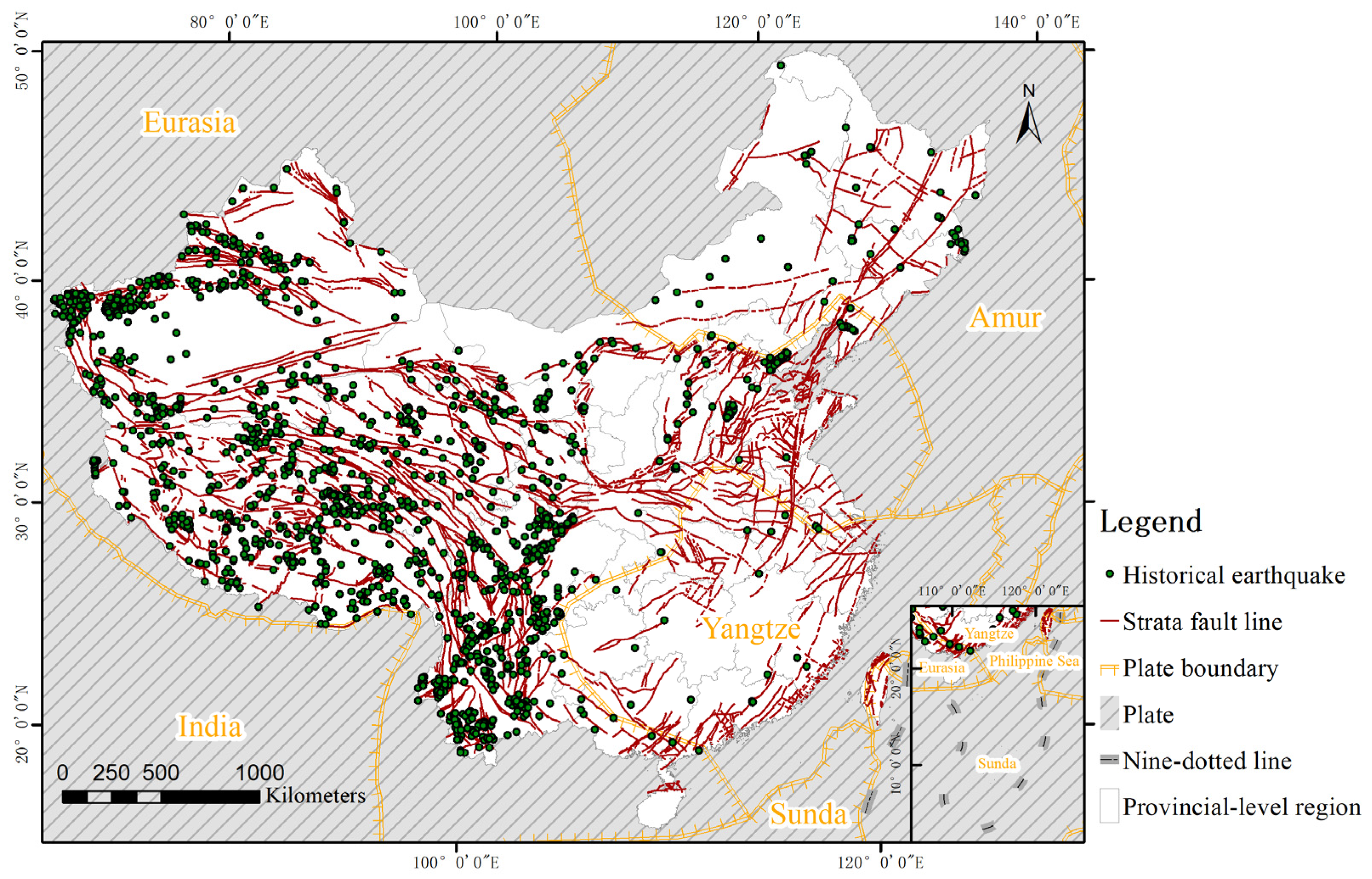
China’s mainland is located at the intersection of the Alpine-Himalayan and Circum-Pacific seismic zones, where destructive earthquakes occur frequently [25]. Seismicity in China’s mainland is characterized by high frequency, wide distribution, great intensity, shallow seismic focus, and clear regional differences. Most earthquakes in this area are shallow focus earthquakes that occurred within the continental crust, whose principal type are strike-slip type [26]. Based on statistical data from the Earthquake Science Knowledge Service System (http://earthquake.ckcest.cn/earthquake_n/dzml/ch5.html, accessed on 15 July 2021), we developed a chart of the spatial distribution of historical earthquakes in China’s mainland. Figure 1 shows the positions of plates and all earthquakes over 4.0 that have occurred in China’s mainland since 1950. These earthquakes are widely distributed in China’s mainland and the spatial pattern of seismic activities in this area is featured by strong activities in the west and weak activities in the east.
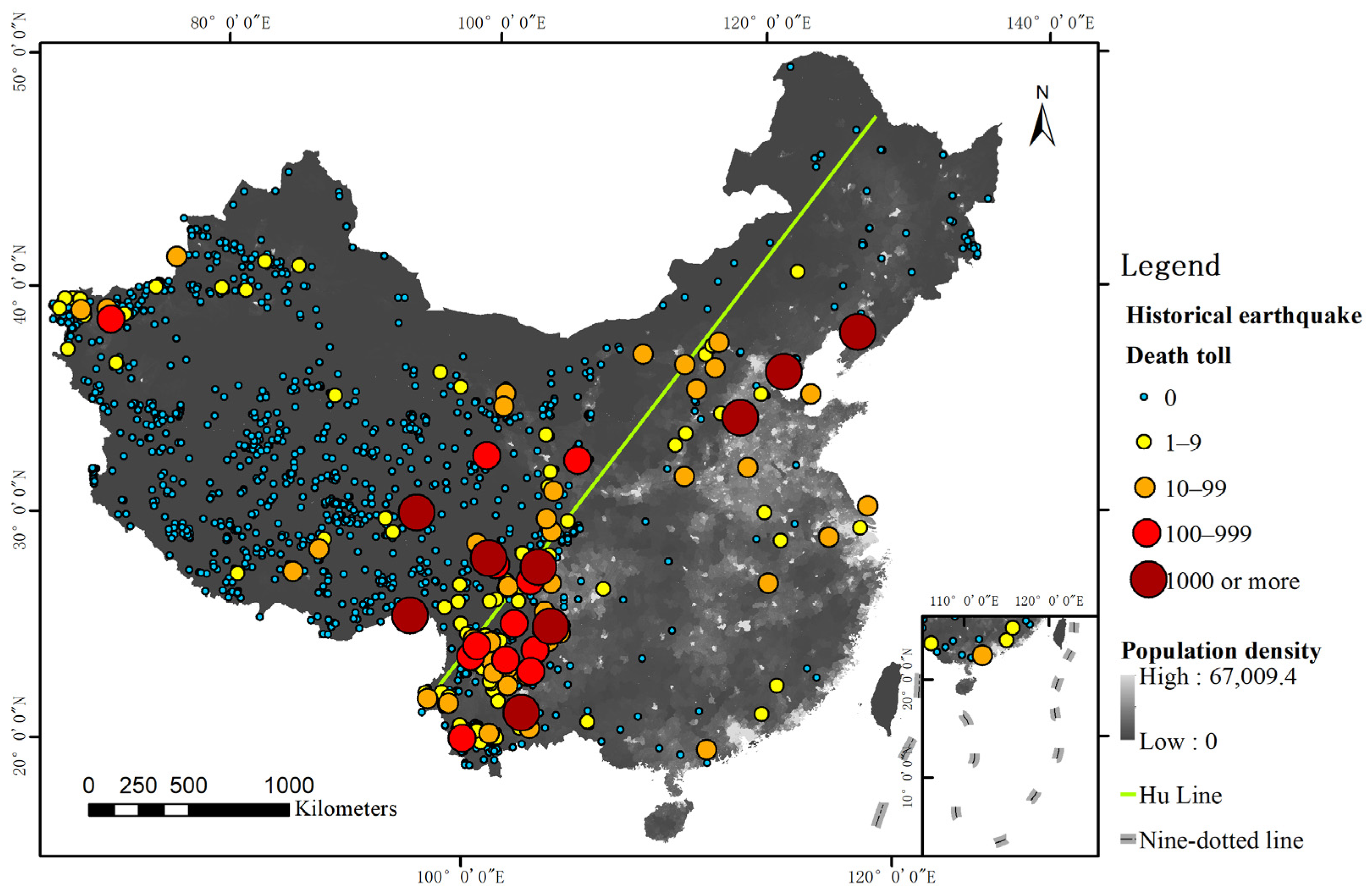
With an area of 9.6 million square kilometers (including Taiwan Province), China has diverse natural and human geographical environments that differ in terms of climates, landforms and geological conditions in China; hence, it is difficult to build a single seismic casualty prediction model that is suitable for the whole area. Seismic destructive effects in this vast area are obviously regional. Figure 2 shows the distribution of population and historical earthquakes in China’s mainland. The frequency of earthquakes and life losses caused by these disasters are roughly bounded by a population dividing line called the Hu Line [27]. To the east of the Hu Line, earthquakes have caused lager death tolls than those to the west of this boundary, although high seismicity has been observed in the west. Since 1949, 19 provinces in China’s mainland suffered deaths due to earthquakes, among which Hebei, Sichuan, and Yunnan Provinces suffered the most life loss events, accounting for more than 90% of all casualties [28].
2.2. Materials
The data that were used in this study included a geological fault dataset, a population dataset and an earthquake case dataset. This study trained and verified the proposed prediction model using the earthquake case dataset, which was also used to evaluate the importance of factors affecting seismic fatality. Geological fault and population datasets were used to divide the study area into defined risk zones based on regional differences.
2.2.1. Earthquake Case Dataset
The majority of the earthquake cases were collected from the Earthquake Science Knowledge Service System (http://earthquake.ckcest.cn/featured_resources/disaster_show.html, accessed on 20 July 2021), which includes 479 records of earthquakes over 4.0 that have occurred in China’s mainland since 1950. We deleted cases without deaths, corrected and supplemented the dataset with relevant literature and reports [29,30,31,32], and finally selected a total of 152 seismic cases with death registers in China’s mainland. The original earthquake case dataset only had attributes such as location, occurrence date, magnitude, focal depth and death toll. Because information about historical earthquakes is very limited and difficult to acquire, a large part of the data mining process was devoted to collecting and supplementing relevant attributes. We complemented the attributes of earthquakes, including epicenter intensity, aftershock, landform, climatic condition, secondary disaster, collapsed buildings and rescue capability, from their disaster situation evaluation reports and relevant literature [24]. The attributes of occurrence time and day were converted from the occurrence date. We calculated the linear density of strata faults in ArcGIS software, and used the statistical analysis tool in ArcGIS to acquire the earthquake attribute of geological fault density. The attributes of population density and the Gross domestic product (GDP) were collected from statistical yearbooks of provinces where earthquakes occurred. GDP is a monetary measure of the market value of all the final goods and services produced in a specific time period. The data we collected is per capital GDP, which is the ratio of GDP to the total population of the earth-quake-stricken region. Detailed information about each attribute in the earthquake case dataset is provided in Table 1.
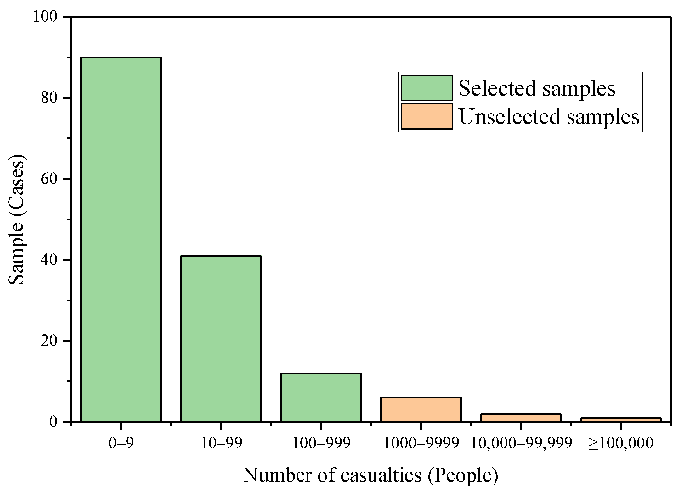
To describe the data distribution characteristics of earthquake cases, we divided their numbers of casualties into 6 categories: 0–9, 10–99, 100–999, 1000–9999, 10,000–99,999, and ≥100,000. Then, we calculated the piecewise frequency statistics for each category and plotted a statistical chart, which is shown in Figure 3. As shown in this graph, the death tolls of most earthquakes in the dataset were within the ranges of less than 10, 10–99 and 100–999. Strong earthquakes with many casualties occurred with lower frequency; hence, this study focuses on accurately predicting the death toll for earthquakes with less than 1000 casualties.
In the construction process of the machine learning model, earthquake samples with many casualties will exert a significant impact on the performance of the prediction model. To evaluate the influence of samples with great values, we conducted an experiment to compare the prediction performance between two data groups: Group A and Group B. Group A was the dataset including all the 152 seismic cases with 1000 casualties or more. Group B was the dataset excluding samples whose numbers of casualties were more than 1000. We took Group A as the training dataset and input it into SVR model, and used the 10-fold cross-validation method to evaluate its prediction performance. The evaluation indicators employed in this experiment were root mean square error (RMSE) and mean absolute error (MeaAE), which are described in detail in Section 6.1. The same experiment was also conducted in Group B. We calculated the average RMSE and MeaAE values for the two groups. The result showed that the RMSE and MeaAE of Group A were 6579.29 and 2346.96, respectively. By contrast, the RMSE and MeaAE of Group B were 48.27 and 40.41 respectively, which means Group B shows significantly better prediction performance due to the exclusion of extreme value samples.
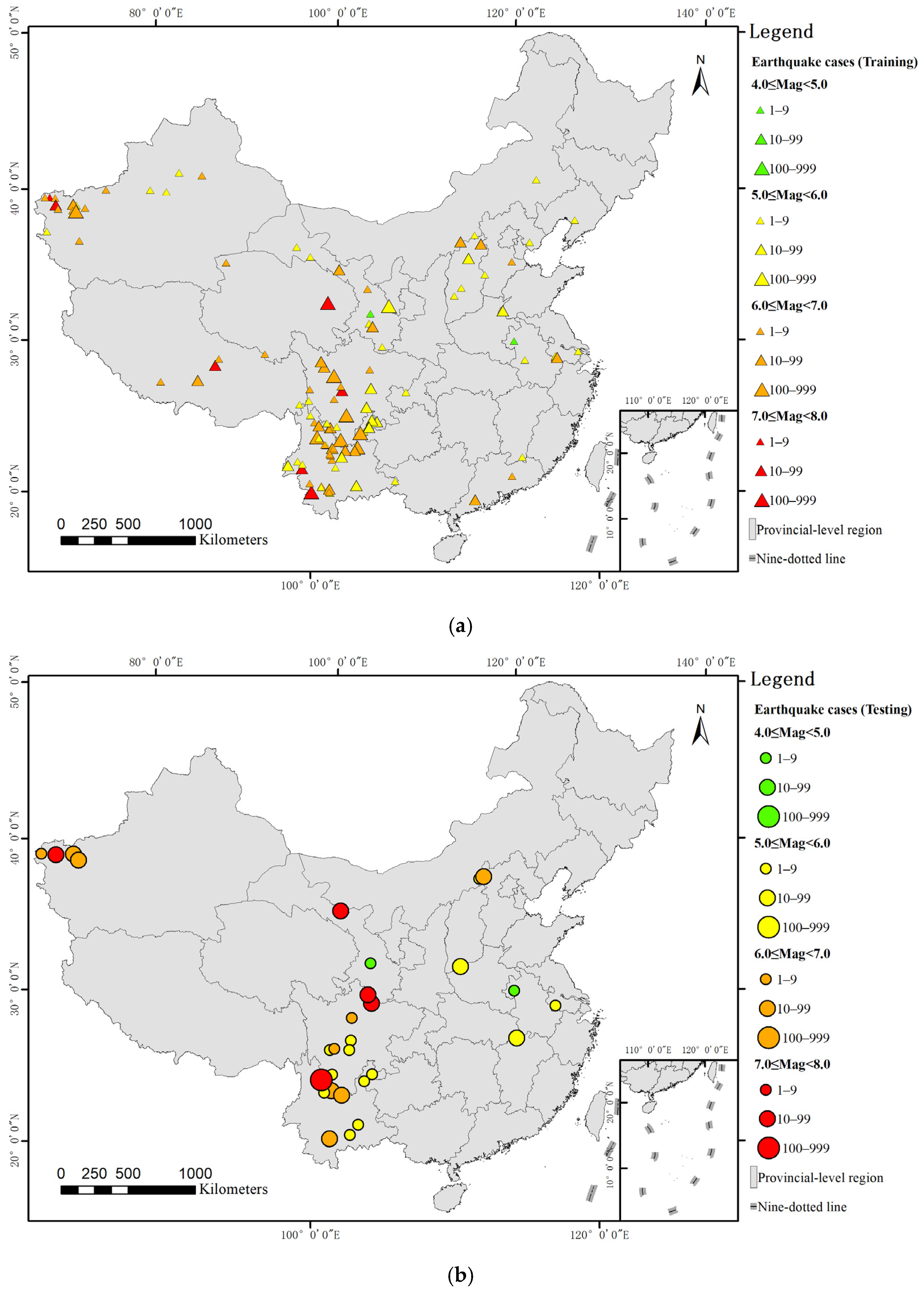
Considering that the devastating earthquakes with more than 1000 casualties occur extremely unfrequently, and their disaster mechanisms are much more complicated, the study focuses on accurately predicting the death toll for earthquakes with less than 1000 casualties. Therefore, we removed cases with more than 1000 casualties in order to avoid the influence of great values. A total of 143 seismic cases with death registers were finally selected. The procedure of dataset division is as follows. (1) In Section 3, we proposes a spatial division method and divides the study area into three groups: high, moderate and low risk zones. Based on the result of spatial division, those selected cases were divided into three parts, including 49 cases in low risk areas, 13 in moderate risk areas, and 81 in high risk areas. (2) To evaluate the prediction accuracy of the Z-SVR model for three degrees of risk zones, we divided the dataset into training and testing datasets. For earthquake cases in each degree of risk zones, we randomly extracted 1/5 of them as the testing dataset, and the remainder was divided into the training dataset. We finally extracted 10 cases in low risk zones, 3 in moderate risk zones, and 17 in high risk zones as the testing dataset to evaluate the performance of the seismic casualty prediction model. The remainder was used as training dataset for building Z-SVR model. Table 2 presents the division of sample dataset. Figure 4 shows the spatial distributions of historical cases.
2.2.2. Geological Fault Dataset
We collected the geological fault dataset from the China Earthquake Data Center (http://datashare.igl.earthquake.cn/map/ActiveFault/introFault.html, accessed on 24 July 2021). It provides the spatial distribution of strata faults in China; the data are in vector format and can be used for spatial analysis in ArcGIS software. This dataset includes 1966 fault segments. For 456 of these segments, detailed parameters such as age, orientation and sliding rate are provided; for 664, only the name and number are specified; for 846, only graphical features are provided, without any attributes. Since the coordinate system of the dataset is the Krassovsky ellipsoid with the Albers projection, we used the projection raster tool in ArcGIS to convert it into the WGS 1984 to ensure the consistency of the spatial reference.
2.2.3. Population Dataset
The population dataset was collected from WorldPop (https://www.worldpop.org/, accessed on 28 July 2021). It details the spatial distribution of the population with a spatial resolution of 100 m. Its units are number of people per pixel with country totals adjusted to match United Nations national population estimates. The format of this dataset is raster, where the digital value of every pixel reflects the total population within this grid. Considering that the samples in the earthquake case dataset have a long time series while population data of a single year have difficulty reflecting demographic changes, we collected population records in China’s mainland every five years from 2000 to 2020 (2000, 2005, 2010, 2015 and 2020) to explore the change in population in a long time series.
2.3. Methods
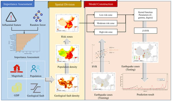
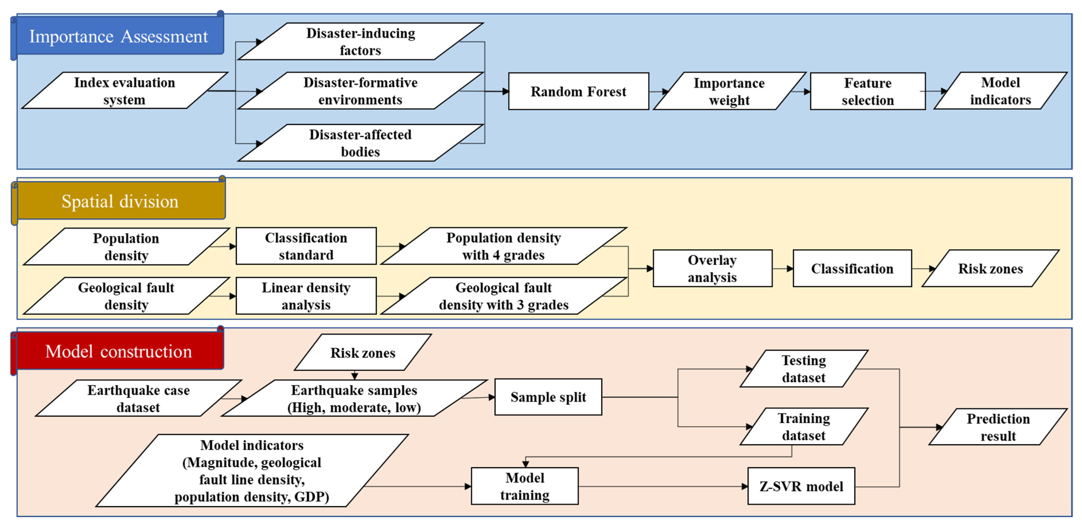
A methodological flowchart of the investigation is shown in Figure 5.
Seismic fatality is a comprehensive result that is influenced by diverse factors, and whether a factor has a decisive impact on earthquake casualties is an essential question for feature selection of prediction models [33]. Therefore, before constructing a prediction model for earthquake casualties, it is crucial to establish a reasonable index system and analyze the importance of relevant indicators, which will serve as a reference for the prediction model to select more important features. Based on regional disaster system theory, this study established an evaluation index system for 14 major features that affect earthquake fatality. We used the earthquake case dataset and the random forest model to assess the importance weights of features, of which the ranking served as an important reference for feature selection of the prediction model.
Because of the variations among regions, there will be different numbers of casualties due to earthquakes with the same ground motion parameter. Therefore, in earthquake cases with the same seismicity, the diversity of disaster-formative environments and disaster-affected bodies reflects the difference among regions [34]. Due to the vast area of China’s mainland, it is difficult to build a universal prediction model that is suitable for all regions. To enhance the accuracy of earthquake disaster assessment in emergency periods, it is effective to divide the study area into risk zones based on regional differences and construct a model that performs well for each risk zone. Based on the results of the importance assessment and feature selection, geological fault density and population density are the most important features of disaster-formative environments and disaster-affected bodies, respectively. Therefore, we chose these two features with relatively high importance weights as representative factors for developing a partition standard and dividing the study area into the defined grades of risk zones. The accuracy and applicability of the earthquake casualty prediction approach can be improved by building different submodels for areas with different regional characteristics.
As an extension of support vector machine (SVM) for solving regression problems support vector regression (SVR) has attracted much attention in the field of machine learning and displayed strong predictive ability in mortality evaluation. Compared with other machine learning algorithms, SVR can achieve the optimal solution with a small number of samples and avoid problems such as overfitting and local extremum as much as possible, which makes its generalization ability and performance stand out [35]. However, as a machine learning method that is based on historical statistics, it may be difficult for the SVR model to accurately predict casualties due to earthquakes occurring in different regions of the study area, especially those with vast acreage and diverse environments. Therefore, based on the characteristics of SVR and regional differences in the study area, we constructed a zoning SVR model (Z-SVR) for various regions in the study area; for which the optimal model parameters for all risk zones were identified using training samples from the earthquake case dataset.
3. Spatial Division
3.1. Importance Assessment
According to regional disaster system theory, a seismic disaster is a complex mechanism that is a comprehensive result of interactions between disaster-inducing factors, disaster-affected bodies and disaster-formative environments [36]. Among them, disaster-inducing factors, such as seismic magnitude and focal depth, are the sufficient conditions for disaster occurrence; disaster-affected bodies, such as population distribution and building destruction, represent the necessary conditions for disaster resilience; and disaster-formative environments, such as climatic condition and secondary disaster, provide a natural and human geological background that affects disaster-inducing factors and disaster-affected bodies [17]. The loss due to a disaster is attributed to the combined effects of these three factors; therefore, for screening the prediction indicators, we constructed an evaluation index system on the basis of regional disaster system theory, which is presented in Table 3.
Determining the importance weights of all features in the evaluation index system is a quantitative task in importance assessment. Although traditional linear models show good performance in the importance assessment of factors that affect earthquake fatality, the result can be easily disturbed by the uncertainty and fuzziness of input data [37]. An integrated ensemble model is an effective approach for mitigating the above problem and improving the accuracy and generalization performance of the evaluation method [38], which was demonstrated by previous studies [39]. Random forest (RF) is an effective integrated ensemble model with random binary decision trees for classification or regression [39]. As an expansion of the bagging method, this algorithm constructs multiple independent estimators that determine the output result by average or majority voting. This approach enhances the precision and stability of the prediction model, reduces the sensitivity of the model to noise and outliers, and avoids problems such as overfitting [40]. In contrast to other machine learning methods, the RF model can provide the quantified importance of prediction indicators by calculating their increases in predictive error by randomly permuting the values of a variable through out-of-bag observations of each tree.
We chose 7 indicators of disaster-inducing factors, 4 of disaster-affected bodies and 3 of disaster-formative environments as the input parameters of the RF model to evaluate their importance to earthquake fatality. The values of the input parameters were extracted from the earthquake case dataset. We utilized the machine learning package scikit-learn of the Python programming language to construct the RF model. The “feature_importances_” is an attribute of the RF model in the scikit-learn package. The importance of a feature is computed as the normalized total reduction of the criterion brought by that feature. The procedure is summarized as follows:
- Inputs: Disaster-inducing factors (7 variables), disaster-affected bodies (4 variables) and disaster-formative environments (3 variables).
- Parameters: Number of estimators = 150, criterion = ‘squared_error’, max depth = 6, min samples split = 2, min samples leaf = 1, min weight fraction leaf = 0.0, max features = ‘auto’, max leaf nodes = None, min impurity decrease = 0.0, bootstrap = Frue, oob score = False, number of jobs = None, random state = None, verbose = 0, warm start = False, ccp_alpha = 0.0, max samples = None.
- Step 1: Use bootstrap sampling to extract subtraining sets from the training set.
- Step 2: Generate the feature subsets by randomly selecting features before node splitting.
- Step 3: Establish decision trees.
- Step 4: Obtain the results for the sample to be tested.
- Step 5: Calculate the importance of the input parameters.
- Output: Importance weight of the prediction indicators.
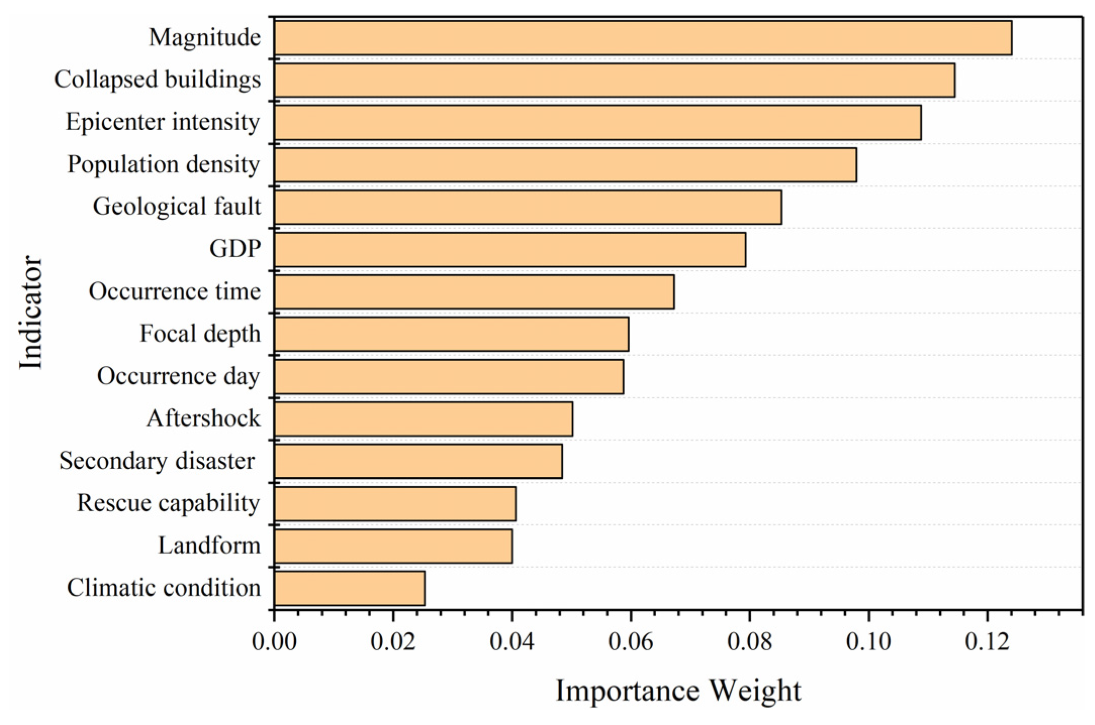
The ranking of all factors according to the importance weights from low to high is shown in Figure 6.
Based on the results of the importance assessment of influential features, magnitude, collapsed buildings, epicenter intensity, population density, geological fault density and GDP are major factors that affect seismic fatality. Magnitude and epicenter intensity are the two most important parameters to depict the severity of an earthquake and exert substantial influence on the seismic fatality; however, there is a strong correlation between these two features. To avoid information redundancy, we selected magnitude, which has greater importance weight, as the input parameter of the Z-SVR model. Building destruction is the direct cause of earthquake injuries and deaths [41], and the primary task of emergency rescue is to search for people who are buried in collapsed constructions. However, the aim of the proposed model in this study is to rapidly predict the possible casualties of an instantly occurring earthquake, which requires an extremely fast response speed. It will take some time to identify the situation of building destruction and count the number of collapsed buildings. Population density is the most important feature among the disaster-affecting bodies; since human beings are the major victims of earthquakes, it is significant to choose this feature as one of the prediction indicators. Geological fault is the most important factor under the level of disaster-formative environments, where the density of strata fault lines can be used to quantitively analyze regional differentiation and merits consideration. GDP is a comprehensive indicator that is mutually restricted with population density in terms of earthquake casualties; therefore, it is significant to introduce this factor as an input parameter and consider its comprehensive effect with population density to ensure the stability and accuracy of the prediction results. In conclusion, based on the result of the importance assessment and the principles of rapid evaluation and avoiding information redundancy, we finally selected magnitude, population density, geological fault density and GDP as the input parameters for the construction of the Z-SVR model, among which geological fault line density and population density were also applied to divide the study area into risk zones.
3.2. Population Density
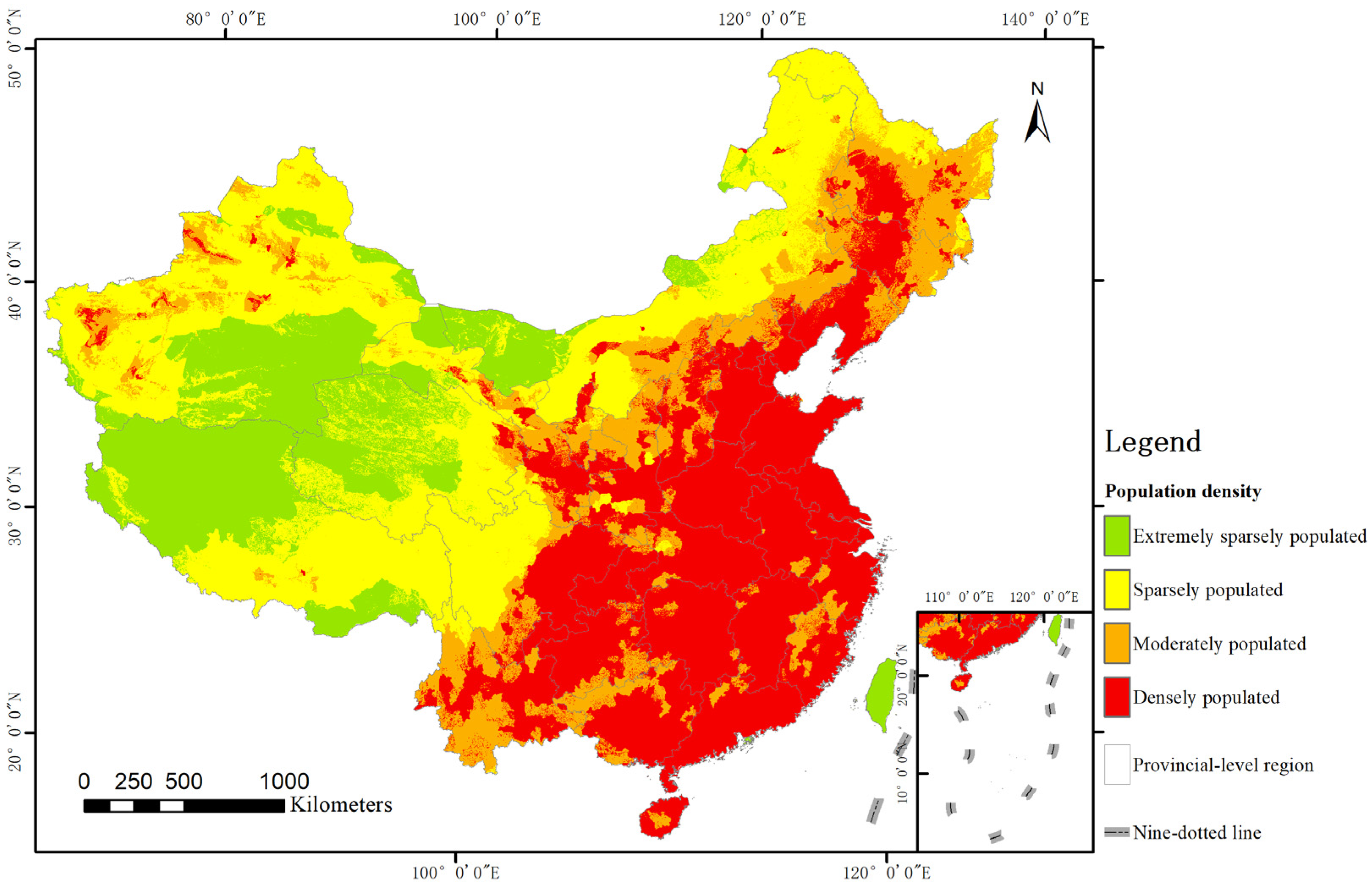
Disaster-affected bodies reflect the necessary conditions for disaster resilience, of which population density has a major influence on the number of earthquake casualties and the degree of destruction. High population density provides a vital motivation for the increase in earthquake casualties [42]. In this study, the population dataset that was collected from WorldPop includes raster data on the population distribution of China’s mainland every five years from 2000 to 2020 (2000, 2005, 2010, 2015 and 2020). For those five raster datasets, we converted the population count value to population density and calculated the average density, which was implemented using the raster calculator tool in ArcGIS software. The general classification standard of population density was used to divide different population densities into four categroies: extremely sparsely (less than 1 people/), sparsely (from 1 to 25 people/), moderately (from 25 to 100 people/), and densely populated (greater than 100). Through this standard, we divided China’s population distribution dataset into four parts, as shown in Figure 7.
3.3. Geological Fault Density
Disaster-formative environments refer to the natural and human geological background that affects disaster-inducing factors and disaster-affected bodies [17], among which geological faults are the zone blocks that bump into each other and generate shakes. Previous work [28] has demonstrated that the distance from a geological fault is correlated with the number of casualties that are caused by an earthquake. Therefore, we calculated the linear densities of strata faults in China using ArcGIS software. The linear densities were divided into three grades (high, moderate and low) by natural breaks. Figure 8 shows the spatial distribution of the classified geological fault densities in the study area.
3.4. Overlay Analysis
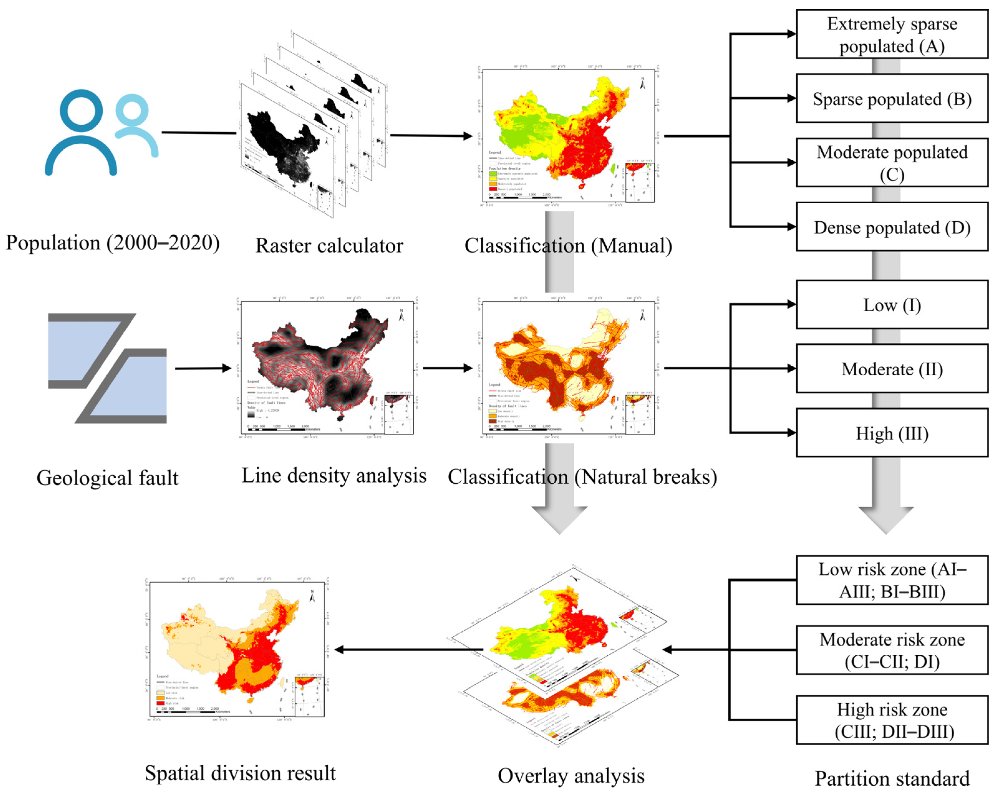
Overlay analysis is a frequently used geographic computing operation and a significant spatial analysis tool in GIS software, which is widely used in applications that are related to spatial computing [43]. This operation integrates different data layers and their corresponding attributes in the study area, which connects multiple spatial objects from multiple data sources and quantitatively analyzes the spatial range and characteristics of the interactions among different forms of spatial objects. Based on the feature selection results, geological faults are the birthplace of an earthquake, and humans are the victims of seismic disasters. In earthquakes with similar seismicity, denser strata fault lines and higher population density will lead to a greater risk to personnel safety [28]. For the above reasons, this study divided the study area into parts according to the variations in population density and strata fault density and established a corresponding partition standard. We developed a comprehensive partition standard that was used to overlay the classification results. Then, we divided the study area into risk areas of three grades: low risk, moderate risk, and high risk zones. The theory and procedure of the proposed spatial division method are illustrated in Figure 9.
4. Prediction Model
4.1. Algorithm
Support vector machine (SVM) is a kind of machine learning method that is based on statistical learning theory and is a supervised learning model [44]. SVM implements the structural risk minimization principle rather than the empirical risk minimization principle [45], which gives it unique advantages in solving small-sample, nonlinear and high-dimensional pattern recognition problems. Although SVM was initially applied to classification problems, it has been gradually used to solve regression problems due to its good performance in function fitting [46]. SVR is an extension of SVM for solving regression problems. Compared with other machine learning algorithms, SVR can obtain the optimal solution with a small number of samples and avoid problems such as overfitting and partial extreme values as much as possible [28], and its generalization ability and performance have been well demonstrated.
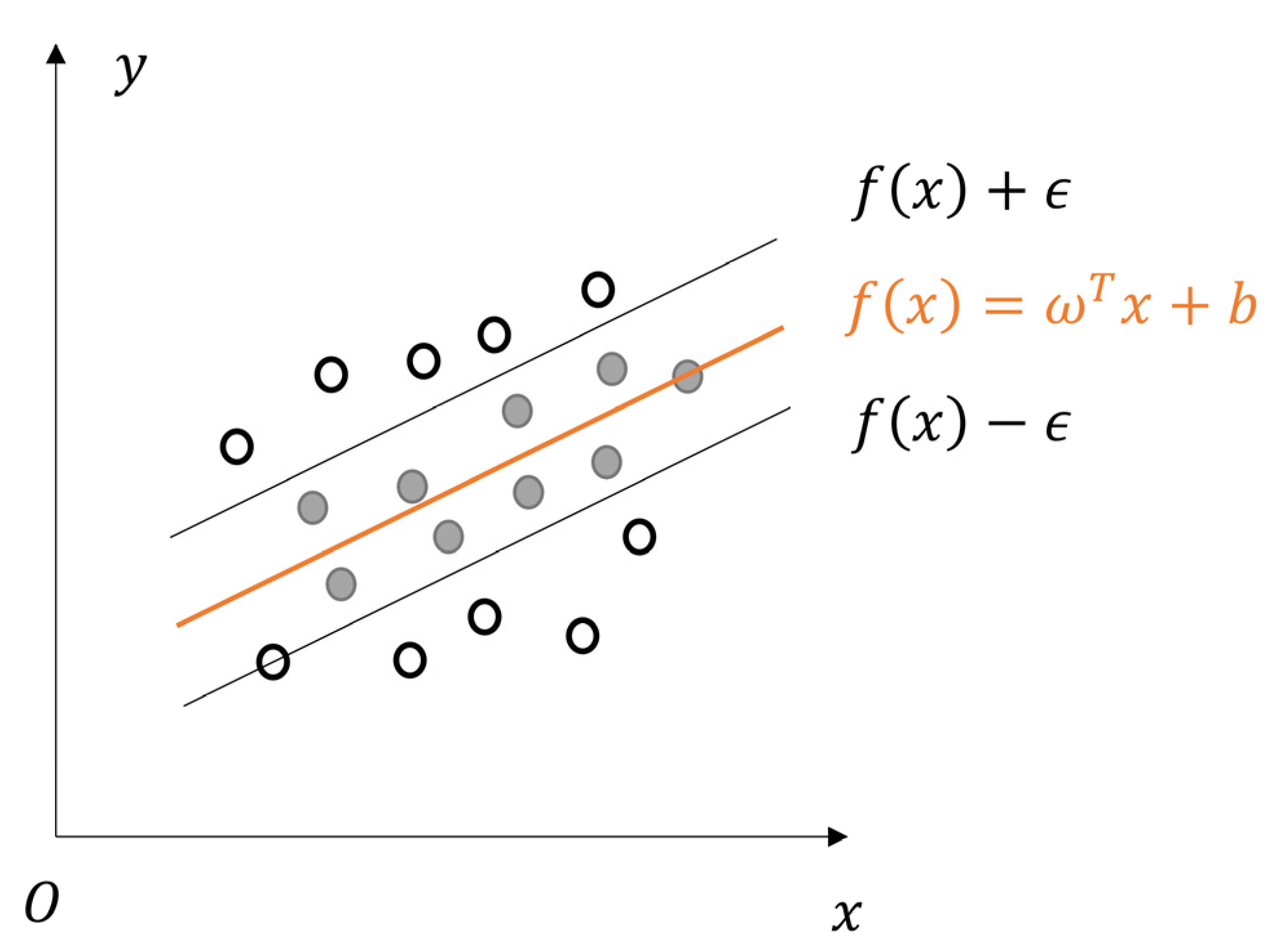
The SVR algorithm is explained as follows. Consider a given training sample set , where , is the th sample and has feature dimensionality , is the value of the th feature, is the corresponding target value of the th sample, and is the number of samples. The goal of SVR is to find a regression model such that is close to its corresponding target value , where and are parameters to be calculated. In the traditional regression model, the function loss is calculated based on the difference between and , which is too strict and will eventually lead to overfitting [47]. To overcome this disadvantage, SVR sets a maximum deviation between and , and the function loss is counted only when the difference between and is greater than (Figure 10). This is equivalent to constructing a spacer band of width with as the center; when the training sample is within the spacer band, the prediction result will be designated as correct [48]. Therefore, the SVR problem can be formulated as
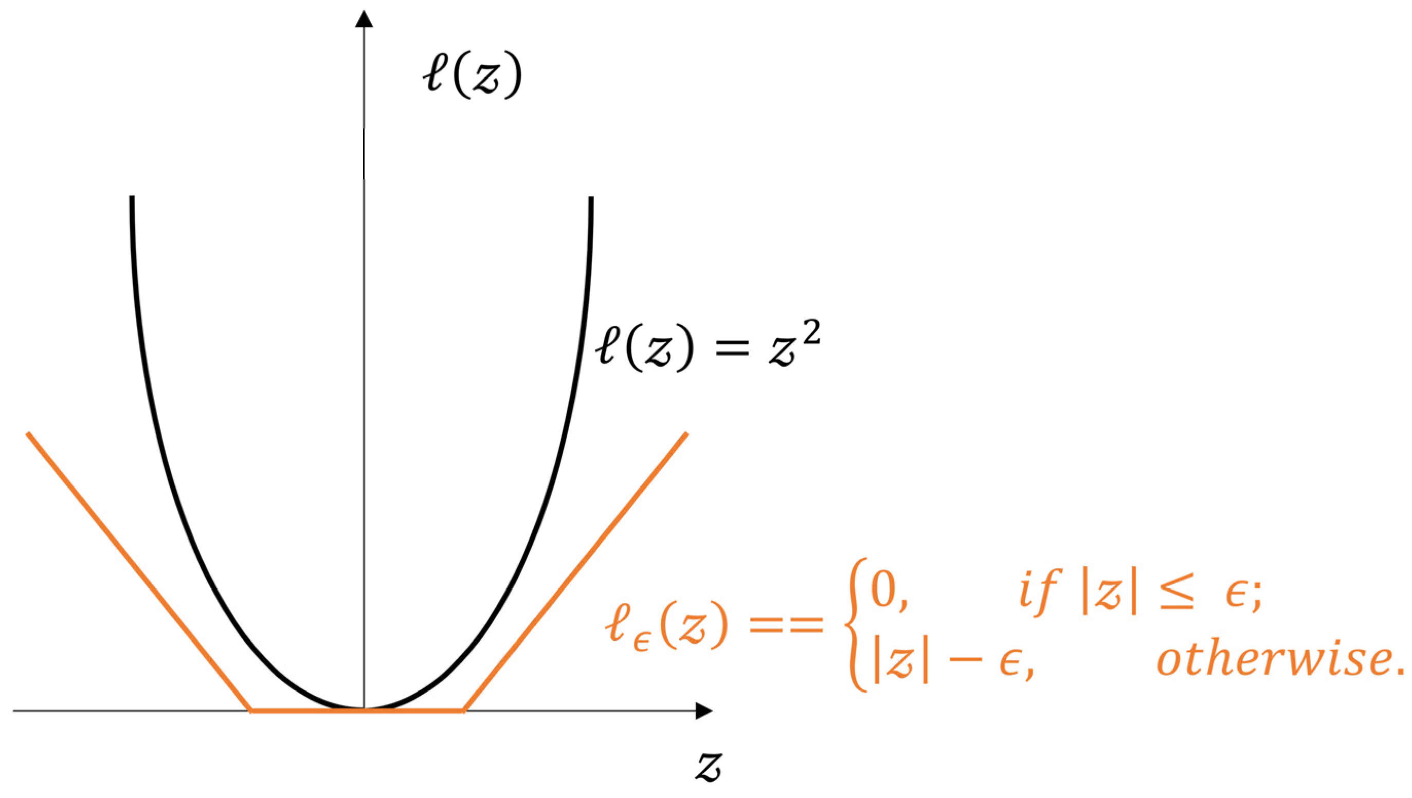
where is a regularization constant and is an -insensitive loss function (Figure 11), which is expressed as
The first term of Equation (1) represents the flatness of the function, which is also called the structural risk, and the second term of the equation, namely, the fitness between and its corresponding target values, which is also called the empirical risk [48]. The regularization constant is a compromise between the structural risk and empirical risk. The constant determines the trade-off between the flatness of and the amount up to which deviations larger than are tolerated [49]. To describe the real deviation, two slack variables, namely, and , are introduced, and Equation (1) can be reformulated as
To efficiently solve the above optimization problem with inequality constraints, multipliers , , , and are introduced. Based on the Lagrange multiplier method, the following function can be deduced from Equation (3):
is substituted into Equation (4), the partial derivatives of with respect to , and are calculated, and these partial derivatives are set equal to 0. The following system of equations is obtained:
After solving the above system of equations, the dual problem of SVR can be formulated as
To solve the above quadratic programming problem, the Karush-Kuhn–Tucker (KKT) conditions [50] are used:
Substituting Equation (5) into yields the following solution of the SVR:
If the term of Equation (11) is not equal to 0, the corresponding sample is a support vector of SVR that is located outside the spacer band. Based on the KKT conditions, it is found that in Equation (10), every sample satisfies the conditions and ; therefore, is equal to 0 when . Then, the value of can be deduced from Equation (11) as
However, Equation (11) is merely a solution for linear SVR. For real-world problems with high feature dimensionality, it is impossible to find a hyperplane that satisfies both fitness and flatness simultaneously [47]. An efficient approach is to map samples from the original space to a higher-dimensional feature space where the samples are linearly separable [48], and Equation (5) can be reformulated as
where is the feature vector after mapping to a higher-dimensional feature space.
With the utilization of the kernel function method, the following solution for nonlinear SVR is obtained:
where is the kernel function. Table 4 presents various widely used kernel functions.
4.2. Model Construction
Based on the results of the importance assessment and feature selection, we selected the magnitude, population density, geological fault density and GDP as the input variables and selected the number of earthquake casualties as the output variable. Considering that different prediction indicators have different units of measurements, it is necessary to normalize the sample dataset to enhance the convergence speed in finding the optimal solution and to improve the accuracy of the Z-SVR model. The normalization method that was used in this study was z-score normalization, which can be formulated as
where is the number of samples in the dataset, . is the initial value of the th sample, is its corresponding normalized value, and is the average initial value of all samples.
Previous studies [51,52] have shown that the type of kernel function and corresponding parameters have substantial impacts on the prediction performance of the SVR model. To construct a fine-tuned Z-SVR model, parameter for the linear kernel, parameters (, gamma) for the Gaussian kernel and sigmoid kernel, and parameters (, gamma, degree) for the polynomial kernel should be selected [47]. is the regularization parameter; gamma and degree are equivalent to and . in Table 4, respectively. Grid search is a general and effective method for parameter optimization, which is usually combined with cross-validation [17]. To find the best SVR model for each risk zone, this study invoked the GridSearchCV module in the scikit-learn package to search for optimal kernel functions and their corresponding model parameters in a specified range based on grid search. The selected parameters of the Z-SVR model are presented in Table 5.
This study obtained the Z-SVR model using the Python programming language and machine learning package scikit-learn. The procedure of model establishment is summarized as follows: (1) Select suitable features as input parameters. (2) Preprocess the sample dataset by normalizing and dividing samples into training data and testing data. (3) Establishing a scoring rule for comparing the predicted results with the actual number of death casualties; if these two values are of the same order of magnitude, the prediction will be considered correct. (4) Invoke the SVR module in the scikit-learn package to build a model for each risk zone. (5) Invoke the GridSearchCV module in the scikit-learn package, and obtain parameters and search ranges; then, use the 10-fold cross-validation method to test the robustness of the model. (6) Input the training dataset into the SVR model for each risk zone to obtain optimal kernel functions and their corresponding model parameters for the Z-SVR model. (7) Input the testing dataset into Z-SVR model and predict the earthquake death tolls. (8) Since the number of earthquake casualties should not be negative, revise negative prediction results by setting them to 0. (9) Assess the performance of the Z-SVR model on the testing dataset.
5. Results
5.1. Spatial Division of the Study Area
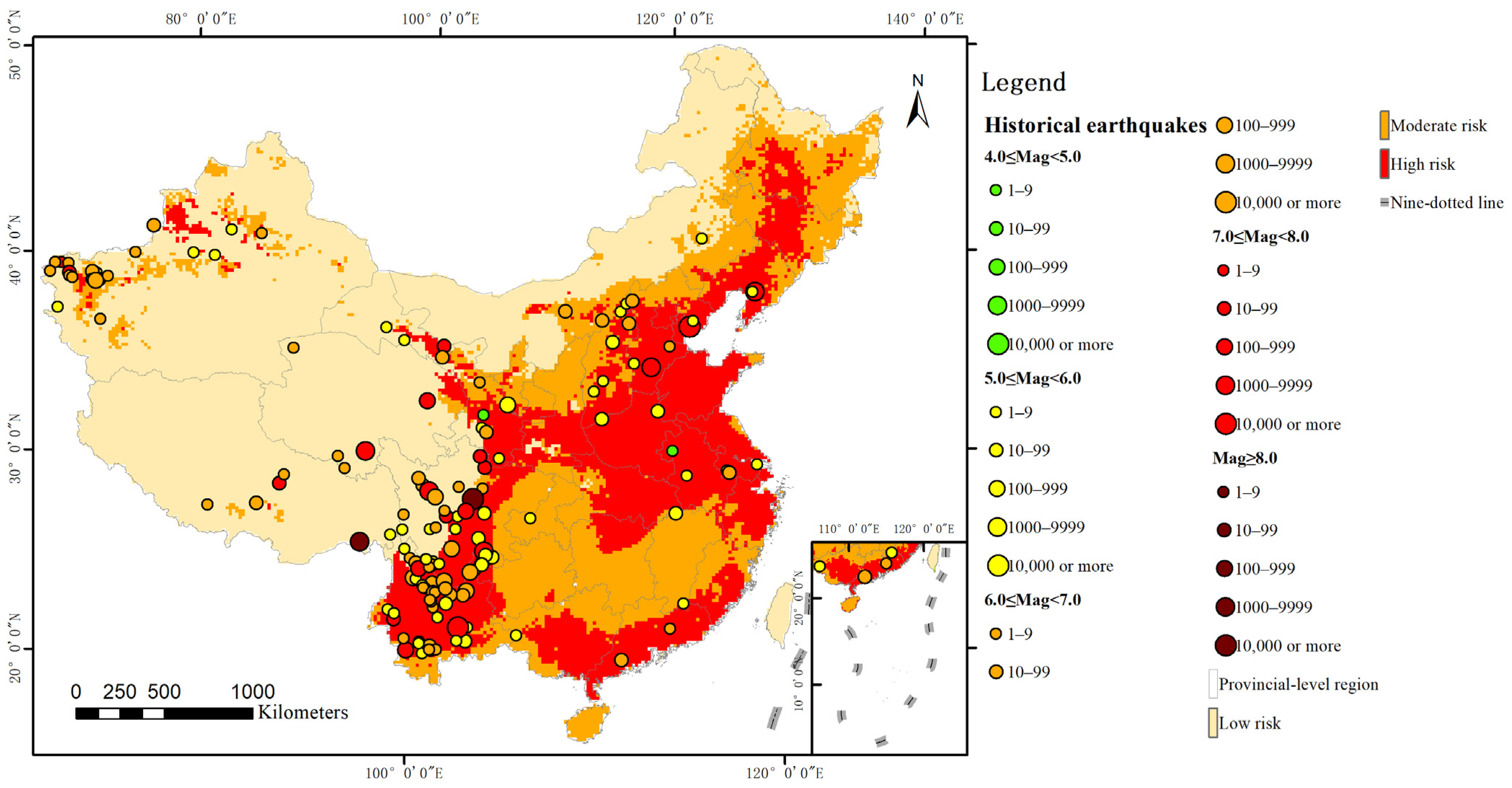
Considering the vast area and diverse environments of China’s mainland, to build an earthquake casualty prediction model with better applicability, it is helpful to propose a machine learning approach with submodels that are applied to different regions. Using the strata fault dataset and population dataset, we divided the study area into risk zones using the raster calculator tool in ArcGIS software according to the proposed partition standard. We plotted the spatial division results and overlaid historical earthquakes with various magnitudes and numbers of casualties onto it, as shown in Figure 12.
As shown in Figure 12, low risk zones were the most extensive, which accounted for 51.94% of China’s mainland, followed by high risk zones, which accounted for 25.59%. The area of moderate risk zones was the smallest, which accounted for 22.47% of the study area. According to the distribution of historical earthquakes, the majority of destructive earthquakes occurred in high risk areas, which indicates the validity of the proposed spatial division method. Fewer destructive earthquakes occurred in some provinces of Northern China (Heilongjiang, Jilin, Beijing and Shanxi), Southern China (Hubei, Hunan and Guizhou) and Eastern China (Zhejiang and Fujian), while these regions were divided into high or moderate risk zones. This can be explained by the presence of dense strata fault lines or high population density in these provinces. Considering that regions with fewer earthquakes usually encounter more casualties due to failure to take necessary precautions for disasters, it is significant for people in high and moderate risk zones to be trained with anti-seismic knowledge and to engage in evacuation practices. Interestingly, although earthquakes occurred in Xizang, Qinghai and Xinjiang Provinces of Western China, most parts of these regions were divided into low risk zones. This inconsistency is due to the low population densities of these provinces, which contain vast depopulated zones; this is supported by the observation that most earthquakes with high seismicity caused minor casualties in low risk zones.
5.2. Prediction Result of Z-SVR Model
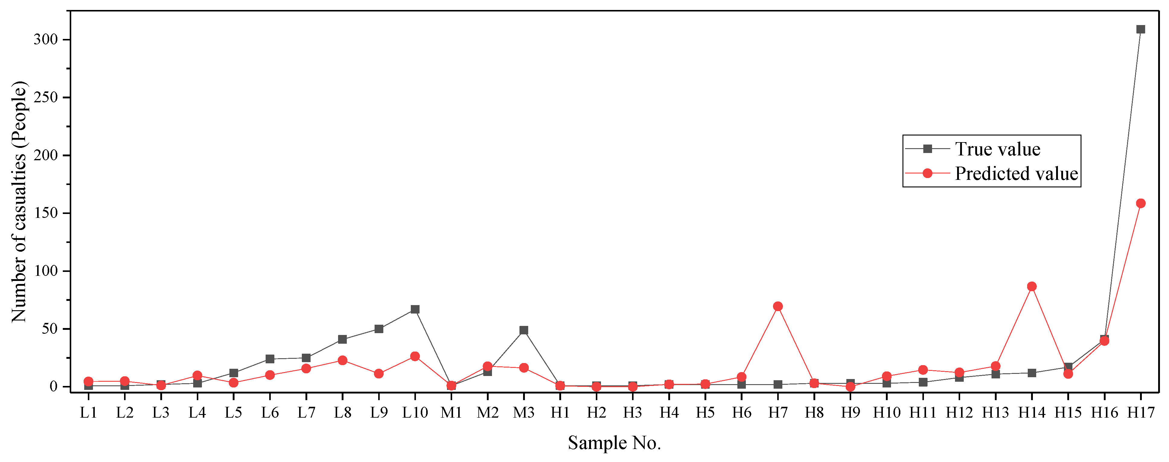
This study improved the SVR model and proposed the Z-SVR model with optimal parameters for different risk areas. We randomly selected 10 samples in low risk zones (L1~L10), 3 in moderate risk zones (M1~M3) and 17 in high risk zones (H1~H17) to predict the numbers of casualties and compare them with corresponding true values, which are presented in Figure 13 and Table 6. Although the number of casualties varied over a large range in the risk zones, the differences between the majority of the predicted values by Z-SVR and the true values were acceptable. However, there were three samples with noticeable error. Among these three earthquake cases, 2 occurred in Puer (H7 and H14), and 1 occurred in Lijiang (H17); both cities are located in Yunnan Province. Considering that Yunnan is a region with significant variation of the geological environment and a huge economic gap between cities and villages, further research should be conducted to develop a specific approach for predicting earthquakes in this region.
6. Discussion
6.1. Comparison between Z-SVR and Other Models
To evaluate the effectiveness of the proposed model, this study selected training samples and used a cross-validation method to evaluate the robustness of the Z-SVR model. The regression and classification performances of the proposed model were also assessed by predicting the numbers of casualties in testing samples and comparing the results in terms of numerical difference and order of magnitude. Similar experiments were also implemented on other widely used machine learning methods, including random forest (RF), back propagation neural network (BP) and logistic regression (LR). This was followed by a series of experiments and detailed analyses.
Several commonly used regression model evaluation indicators were employed in this study, including root mean square error (RMSE) and mean absolute error (MeaAE), which are defined as follows:
where is the predicted death toll of the th sample, is the corresponding true death toll, and is the number of samples.
The classification model evaluation indicators that were applied in this study were , and , which are defined as follows:
where is the number of true-positive samples, is the number of false-positive samples, is the number of true-negative samples, and is the number of false-negative samples.
6.1.1. Cross-Validation
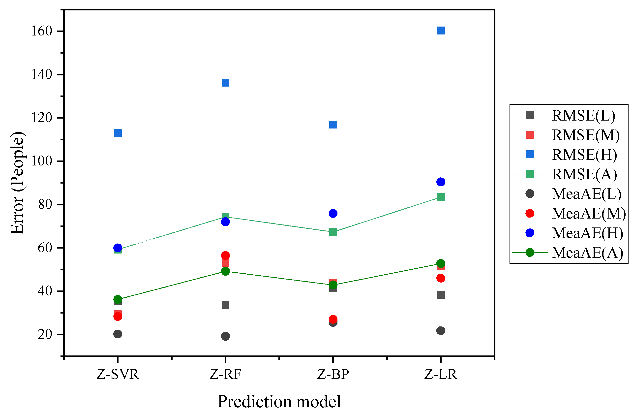
The robustness of each model was evaluated using the cross-validation method. As discussed in Section 2.2.1, 113 seismic cases were selected as the training dataset, among which 49 cases were in low risk areas, 13 in moderate risk areas, and 81 in high risk areas. We randomly divided the cases in low and high risk zones into ten groups, respectively; considering the limited number of samples, we randomly divided the cases in moderate risk zones into five groups. The sample data in each group were not repeated. We used RMSE and MeaAE to compare the regression precision between the Z-SVR model and other machine learning models using the spatial division method. RMSE and MeaAE were calculated for three degrees of risk zones (L, M and H) and the average values (RMSE(A) and MeaAE(A)) were also given. The comparison result of all models is shown in Figure 14.
Judging from the stability of the prediction results on the training samples, all models performed relatively better in low and moderate risk zones than in high risk zones. A possible explanation is that there are 64 training samples in high risk zones, much more than in low and moderate risk zones. In addition, the true numbers of casualties in these 64 samples vary from 1 to 748, which is a huge range and increases the difficulty for machine learning models to achieve accurate prediction. Among all prediction models, Z-LR performed the worst, as its RMSE and MeaAE were 83.37 and 52.72, respectively, which ranked last in the two evaluation indicators. Z-BP and Z-RF outperformed the Z-LR model, with RMSEs of 67.30 and 74.27, respectively, and MeaAEs of 42.80 and 49.17, respectively. In contrast to the above prediction methods, Z-SVR showed higher overall accuracy in cross-validation experiments for all risk zones. Its RMSE was 59.15, and its MeaAE was 36.16, which were significantly lower than those of the compared models; this indicates that the proposed Z-SVR model had the smallest dispersion and the highest stability.
6.1.2. Regression Accuracy Evaluation
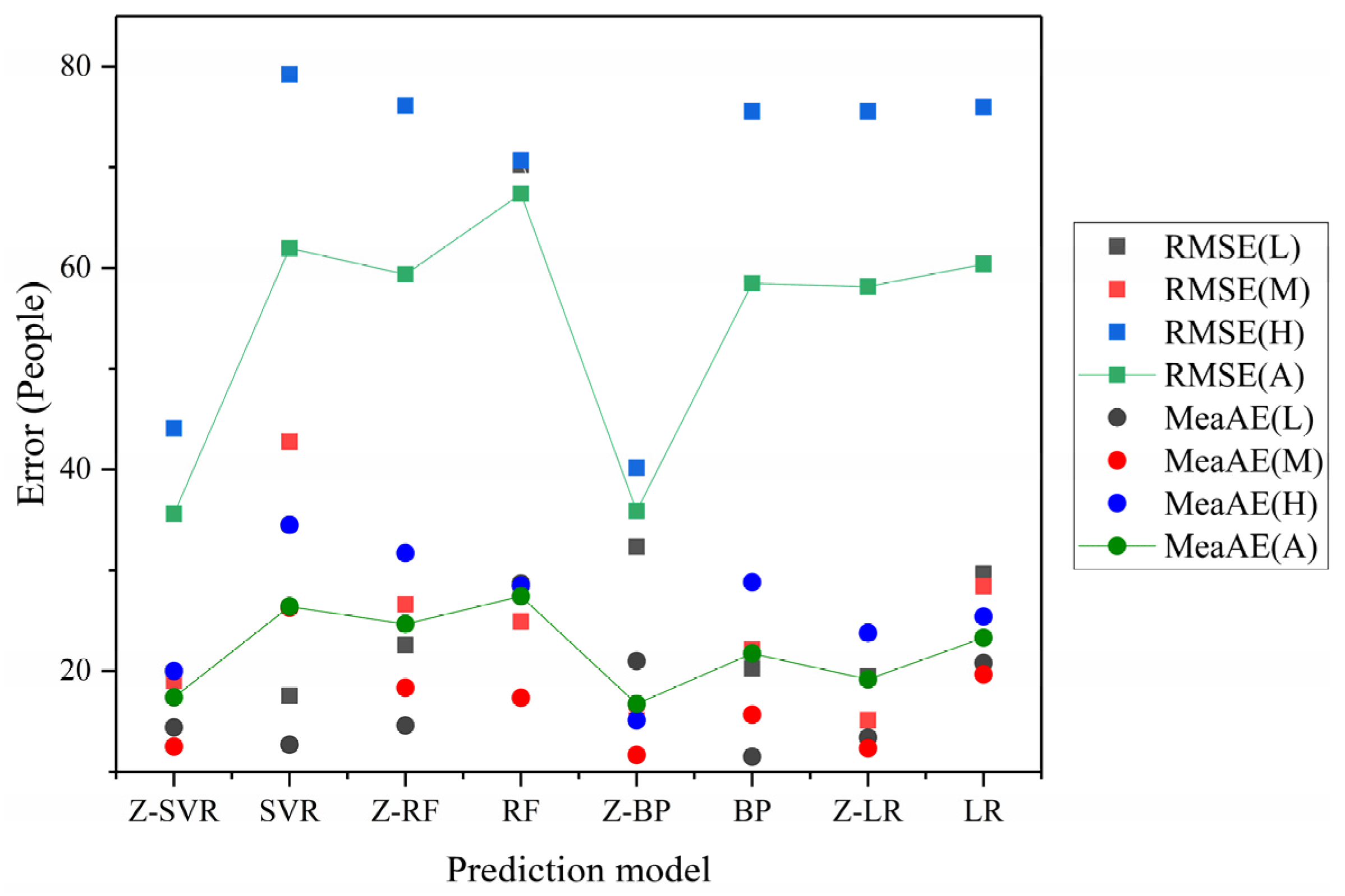
For samples in low, moderate and high risk zones, this study used Z-SVR and other models to predict their death tolls. Evaluation indicators of RMSE (L, M and H) and MeaAE (L, M and H) were calculated for the risk zones, and the overall regression performances (RMSE(A) and MeaAE(A)) of all models were also calculated, which are plotted in Figure 15. For samples in low and moderate risk zones, the majority of models showed relatively high regression accuracy, while for those in high risk zones, the Z-SVR and Z-BP models showed good regression performance. Among all prediction models, in terms of overall MeaAE, the Z-BP model showed the best regression accuracy with the lowest value of 16.73, and the Z-SVR model also performed well with MeaAE(A) of 17.39. In terms of the overall RMSE, the average value of Z-SVR was 35.61, which was the lowest value, followed by 35.89 for Z-BP. The precision evaluation results from Figure 15 further prove that the proposed spatial division method has the advantages of enhancing prediction accuracy and stability. For example, the RMSE of the Z-SVR model was the lowest, namely, nearly half that of the SVR model; a similar result was obtained between the Z-BP and BP models. In addition, the best fitting results were obtained by the Z-SVR and Z-BP models, while the worst results were obtained by the RF, SVR and LR models, among which the SVR and BP algorithms showed obviously improved performance with the utilization of the spatial division method. The above analysis demonstrates that spatial division is an effective method for improving the performance of machine learning algorithms in predicting earthquake casualties and that the proposed Z-SVR model showed good and stable performance in casualty prediction.
6.1.3. Classification Accuracy Evaluation
The prediction results of Z-SVR, Z-RF, Z-BP, Z-LR and their initial models were also compared with the corresponding true values in terms of classification performance, where pairs of prediction and true values with the same order of magnitude were considered correct. Based on this criterion, we calculated the evaluation indicators of , , and for all prediction models for the risk zones, which are presented in Table 7. In low and moderate risk zones, although the of the LR model was 1, its performance was unsatisfactory, which led to a low value; compared with LR and other models, Z-SVR showed better classification performance in low and moderate risk areas with relatively high values and the highest and values. With regard to samples in high risk zones, Z-BP was the model with the best prediction performance, with an value of 0.87. However, the classification result of Z-SVR in high risk zones was also excellent, with the highest , the second-highest and the third-highest values. In general, the Z-SVR model showed significant stability in classification prediction, with the highest values of and and a relatively high value of . The order of Z-SVR in all risk areas from high to low is moderate, low, and high risk zones. However, only a few earthquakes with casualties occurred in moderate risk areas; hence, we obtained a limited number of historical cases for training prediction models and verifying their performances, which made it difficult to evaluate the difference in classification performance order between the two models.
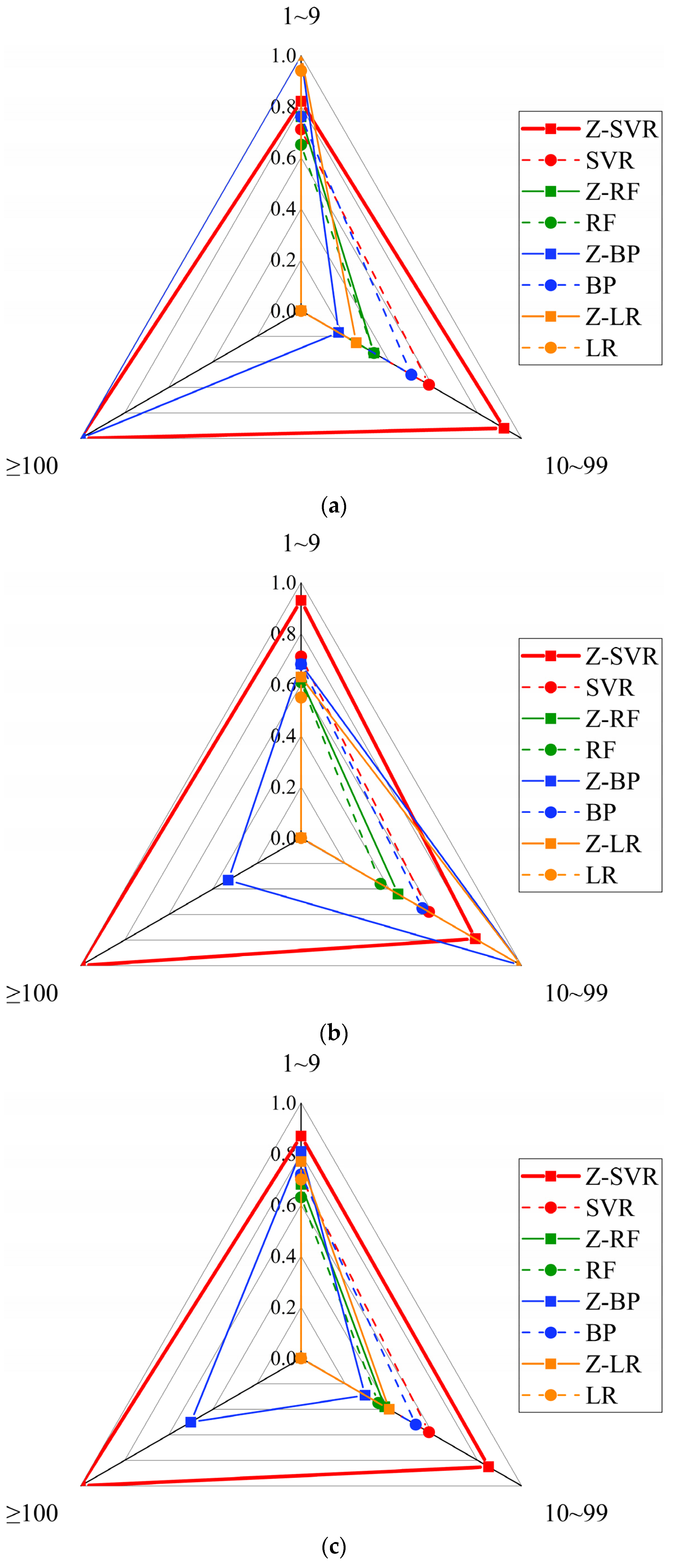
We also divided the testing samples into three groups according to the number of casualties, where the division criterion was order of magnitude (1 to 9, 10 to 99, 100 and greater). We compared the classification performances of Z-SVR and other models in the groups and calculated the evaluation indicators of , , and for all prediction models. Figure 16 presents the comparison results of classification performance between Z-SVR and other models on samples with various numbers of casualties. Z-SVR provided the most balanced and accurate classification into the three groups. Although models such as Z-BP and Z-LR showed better classification performance in terms of or in some groups, the and values of the Z-SVR model in the three groups were high, balanced and stable; thus, Z-SVR had the highest values in each group. In general, the Z-SVR model was the most precise and stable model, which provided accurate classification results for earthquakes with various numbers of casualties.
6.2. Future Work
Further extensive studies are needed, and recommendations for future research are discussed as follows. First, this study analyzes the importance of features that affect seismic mortality, which simply collects 14 features and classifies them into disaster-inducing factors, disaster-affected bodies and disaster-formative environments. Future studies can extend the research by refining the classification standard and increasing the number of factors. Second, this study divides the study area into risk zones of three grades based on regional differences, where the partition standard exerts a potential influence on the accuracy and applicability of the proposed model. Future studies can explore more reasonable criteria for different study areas. Third, the proposed prediction approach is a regression model that is based on SVR, which is essentially a data-driven model. Future studies can build models based on deeper seismic mechanisms to predict deaths that are caused by earthquakes.
7. Conclusions
This study evaluated the importance of 14 features that affect seismic fatality based on the RF model. On the basis of the importance assessment, we selected magnitude, population density, geological fault density and GDP as the input parameters of the prediction model, among which the densities of population and geological faults were also integrated for spatial division. This study also proposed a spatial division method based on the theory of regional difference. We studied the regional diversity of geological fault density and population in China’s mainland using the WorldPop population dataset (100 m resolution) every five years from 2000 to 2020 and the strata fault line dataset and, finally, divided the study area into zones of various risk grades by overlay analysis. Based on the results of feature selection and spatial division, this study proposed a zoning prediction model based on SVR. Using 113 samples in the earthquake case dataset, we implemented model training and obtained the optimal model parameters for each risk zone to enhance the prediction accuracy of earthquake death tolls. The following conclusions were drawn from the results that were obtained in this study:
- Among all selected features from the evaluation index system, the order of importance from high to low is as follows: magnitude, collapsed buildings, epicenter intensity, population density, geological fault density, GDP, occurrence time, focal depth, occurrence day, aftershock, secondary disaster, rescue capability, landform, and climatic condition.
- The proposed method of spatial division based on regional diversity could be used as an effective tool to refine complex study areas. Using this method, we divided China’s mainland into high, moderate, and low risk zones, which laid the foundation for the construction of a prediction model with submodels that are suitable for different risk zones. The verification results demonstrated that the proposed division method is feasible for classifying study regions, especially those with vast area and complex environments.
- The proposed Z-SVR model realizes accurate prediction and good generalization performance. We collected 143 historical earthquake cases, of which 113 cases were selected as the training dataset and 30 for examining the prediction performance of the model. The best model parameters were selected for each risk zone, which led to precise prediction results in risk zones of various grades. The proposed model also showed accurate regression and classification accuracy in the various risk zones compared with other machine learning models, including RF, BP and LR. Moreover, the proposed Z-SVR model was compared to the initial SVR model using the same database. Similar experiments were also implemented on comparative machine learning models, and we found that the prediction performances of all models with spatial division significantly improved. The above results prove the advantages and significance of the proposed model and spatial division method.
Author Contributions
B.L. and T.Z. implemented the research and wrote the original manuscript. A.G. provided the original idea for the study and supervised the research. W.B., C.X. and Z.H. aided with the manuscript revision. All authors have read and agreed to the published version of the manuscript.
Funding
This research was jointly supported by the National Key Research and Development Program of China (Grant No. 2019YFE01277002, No. 2017YFB0504102 and No. 2017YFC1502704) and the National Natural Science Foundation of China (41671412).
Institutional Review Board Statement
Not applicable.
Informed Consent Statement
Not applicable.
Data Availability Statement
Our research data are from relevant open data websites, which can be obtained according to the links listed in our references.
Acknowledgments
The authors would like to express deep gratitude to Jianghong Zhao from Beijing University of Civil Engineering and Architecture for her guidance on the framework design of the paper.
Conflicts of Interest
The authors declare no conflict of interest.
References
- Zhang, Y.; Weng, W.G.; Huang, Z.L. A scenario-based model for earthquake emergency management effectiveness evaluation. Technol. Forecast. Soc. 2018, 128, 197–207. [Google Scholar] [CrossRef]
- Alizadeh, M.; Zabihi, H.; Rezaie, F.; Asadzadeh, A.; Wolf, I.D.; Langat, P.K.; Khosravi, I.; Beiranvand Pour, A.; Mohammad Nataj, M.; Pradhan, B. Earthquake Vulnerability Assessment for Urban Areas Using an ANN and Hybrid SWOT-QSPM Model. Remote Sens. 2021, 13, 4519. [Google Scholar] [CrossRef]
- Schilling, J.; Hertig, E.; Tramblay, Y.; Scheffran, J. Climate change vulnerability, water resources and social implications in North Africa. Reg. Environ. Chang. 2020, 20, 15. [Google Scholar] [CrossRef] [Green Version]
- Yariyan, P.; Zabihi, H.; Wolf, I.D.; Karami, M.; Amiriyan, S. Earthquake risk assessment using an integrated Fuzzy Analytic Hierarchy Process with Artificial Neural Networks based on GIS: A case study of Sanandaj in Iran. Int. J. Disaster Risk Re. 2020, 50, 101705. [Google Scholar] [CrossRef]
- Jian, W. The Research of Earthquake Information Extraction and Assessment Based on Object-Oriented Technology with Remotely-Sensed Data. Doctor’s Thesis, Wuhan University, Wuhan, China, 5 June 2010. [Google Scholar]
- Zhu, Y.; Diao, F.; Fu, Y.; Liu, C.; Xiong, X. Slip rate of the seismogenic fault of the 2021 Maduo earthquake in western China inferred from GPS observations. Sci. China Earth Sci. 2021, 64, 1363–1370. [Google Scholar] [CrossRef]
- Chen, L.; Huang, Y.; Bai, R.; Chen, A. Regional disaster risk evaluation of China based on the universal risk model. Nat. Hazards 2017, 89, 647–660. [Google Scholar] [CrossRef]
- Zhou, W.; Guo, S.; Deng, X.; Xu, D. Livelihood resilience and strategies of rural residents of earthquake-threatened areas in Sichuan Province, China. Nat. Hazards 2021, 106, 255–275. [Google Scholar] [CrossRef]
- National Earthquake Emergency Plan. Available online: http://www.gov.cn/yjgl/2012-09/21/content_2230337.htm (accessed on 17 May 2021).
- Maqsood, S.T.; Schwarz, J. Estimation of Human casualties from earthquakes in Pakistan—An engineering approach. Seismol. Res. Lett. 2011, 82, 32–41. [Google Scholar] [CrossRef]
- Guangxian, X. Rapid assessment of disaster losses in post-earthquake. J. Catastrophology 1991, 4, 12–17. [Google Scholar]
- Jaiswal, K.; Wald, D. An empirical model for global earthquake fatality estimation. Earthq. Spectra 2010, 26, 1017–1037. [Google Scholar] [CrossRef] [Green Version]
- ATC. Earthquake Damage Evaluation Data for California (ATC-13); Applied Technology Commission: Redwood City, CA, USA, 1985. [Google Scholar]
- Ceferino, L.; Kiremidjian, A.; Deierlein, G. Probabilistic model for regional multiseverity casualty estimation due to building damage following an earthquake. ASCE-ASME J. Risk Uncertain. Eng. Syst. Part A Civil. Eng. 2018, 4, 4018023. [Google Scholar] [CrossRef]
- Xianfu, B.; Gaozhong, N.; Yuqian, D.; Qingkun, Y.; Weidong, L.; Liaoyuan, Y. Modeling and Testing Earthquake-induced Landslide Casualty Rate Based on a Grid in a Kilometer Scale: Taking the 2014 Yunnan Ludian MS6. 5 Earthquake as a Case. J. Seismol. Res. 2021, 44, 87–95. [Google Scholar]
- Stav, S.; Lena, N.; Yaron, B.D.; Limor, A.D.; Asim, Z. An Integrated and Interdisciplinary Model for Predicting the Risk of Injury and Death in Future Earthquakes. PLoS ONE 2016, 11, e151111. [Google Scholar]
- Cui, S.; Yin, Y.; Wang, D.; Li, Z.; Wang, Y. A stacking-based ensemble learning method for earthquake casualty prediction. Appl. Soft Comput. 2020, 101, 107038. [Google Scholar] [CrossRef]
- Gao, Z.; Li, Y.; Shan, X.; Zhu, C. Earthquake Magnitude Estimation from High-Rate GNSS Data: A Case Study of the 2021 Mw 7.3 Maduo Earthquake. Remote Sens. 2021, 13, 4478. [Google Scholar] [CrossRef]
- Karimzadeh, S.; Miyajima, M.; Hassanzadeh, R.; Amiraslanzadeh, R.; Kamel, B. A GIS-based seismic hazard, building vulnerability and human loss assessment for the earthquake scenario in Tabriz. Soil. Dyn. Earthq. Eng. 2014, 66, 263–280. [Google Scholar] [CrossRef]
- Feng, T.; Hong, Z.; Fu, Q.; Ma, S.; Jie, X.; Wu, H.; Jiang, C.; Tong, X. Application and prospect of a high-resolution remote sensing and geo-information system in estimating earthquake casualties. Nat. Hazards Earth Syst. Sci. 2014, 1, 7137–7166. [Google Scholar] [CrossRef] [Green Version]
- Wenjuan, Z. Design of the Population Casualty Acquisition and Evaluation System in Earthquake Disaster Areas Based on Mobile Communication Big Data. China Earthq. Eng. J. 2019, 41, 1066–1071. [Google Scholar]
- Huang, X.; Zhou, Z.; Wang, S. The prediction model of earthquake casuailty based on robust wavelet v-SVM. Nat. Hazards 2015, 77, 717–732. [Google Scholar]
- Gul, M.; Guneri, A.F. An artificial neural network-based earthquake casualty estimation model for Istanbul city. Nat. Hazards 2016, 84, 2163–2178. [Google Scholar] [CrossRef]
- Jia, H.; Lin, J.; Liu, J. An Earthquake Fatalities Assessment Method Based on Feature Importance with Deep Learning and Random Forest Models. Sustainability 2019, 11, 2727. [Google Scholar] [CrossRef] [Green Version]
- Sousa, J.J.; Liu, G.; Fan, J.; Perski, Z.; Steger, S.; Bai, S.; Wei, L.; Salvi, S.; Wang, Q.; Tu, J. Geohazards Monitoring and Assessment Using Multi-Source Earth Observation Techniques. Remote Sens. 2021, 13, 4269. [Google Scholar] [CrossRef]
- Shi, P. Natural Disasters in China; Springer: Berlin/Heidelberg, Germany, 2016. [Google Scholar]
- Wen, L.; Wenkai, C.; Zhonghong, Z. Assessing the applicability of life vulnerability models for earthquake disasters in typical regions of China. J. Beijing Norm. Univ. 2019, 55, 284–290. [Google Scholar]
- Tingting, Z. Assessment of Earthquake Fatality and Disaster Degree Based on Spatio-Temporal Method. Bachelor’s Thesis, Beijing Normal University, Beijing, China, 3 June 2020. [Google Scholar]
- China Earthquake Administration. Compilation of Earthquake Disaster Loss Assessment in China’s Mainland; Seismological Press: Beijing, China, 1996. [Google Scholar]
- Monitoring and Forecasting Department of China Earthquake Administration. Compilation of Earthquake Disaster Loss Assessment in China’s Mainland; Seismological Press: Beijing, China, 2001. [Google Scholar]
- Earthquake Emergency Rescue Department of China Earthquake Administration. Compilation of Earthquake Disaster Loss Assessment in China’s Mainland from 2001 to 2005; Seismological Press: Beijing, China, 2010. [Google Scholar]
- Earthquake Emergency Rescue Department of China Earthquake Administration. Compilation of Earthquake Disaster Loss Assessment in China’s Mainland from 2006 to 2010; Seismological Press: Beijing, China, 2015. [Google Scholar]
- Liang, S.; Chen, D.; Li, D.; Qi, Y.; Zhao, Z. Spatial and Temporal Distribution of Geologic Hazards in Shaanxi Province. Remote Sens. 2021, 13, 4259. [Google Scholar] [CrossRef]
- Hoffmann, S.; Beierkuhnlein, C. Climate change exposure and vulnerability of the global protected area estate from an international perspective. Divers. Distrib. 2020, 26, 1496–1509. [Google Scholar] [CrossRef]
- Xiong, K.; Adhikari, B.R.; Stamatopoulos, C.A.; Zhan, Y.; Wu, S.; Dong, Z.; Di, B. Comparison of different machine learning methods for debris flow susceptibility mapping: A case study in the Sichuan Province, China. Remote Sens. 2020, 12, 295. [Google Scholar] [CrossRef] [Green Version]
- Peijun, S. Theory on Disaster Science and Disaster Dynamics. J. Nat. Disasters 2002, 11, 1–9. [Google Scholar]
- Chen, W.; Shirzadi, A.; Shahabi, H.; Ahmad, B.B.; Zhang, S.; Hong, H.; Zhang, N. A novel hybrid artificial intelligence approach based on the rotation forest ensemble and naïve Bayes tree classifiers for a landslide susceptibility assessment in Langao County, China. Geomat. Nat. Hazards Risk 2017, 8, 1955–1977. [Google Scholar] [CrossRef] [Green Version]
- Altmann, A.; Toloşi, L.; Sander, O.; Lengauer, T. Permutation importance: A corrected feature importance measure. Bioinformatics 2010, 26, 1340–1347. [Google Scholar] [CrossRef] [PubMed]
- Chen, W.; Sun, Z.; Han, J. Landslide susceptibility modeling using integrated ensemble weights of evidence with logistic regression and random forest models. Appl. Sci. 2019, 9, 171. [Google Scholar] [CrossRef] [Green Version]
- Stumpf, A.; Kerle, N. Object-oriented mapping of landslides using Random Forests. Remote Sens. Environ. 2011, 115, 2564–2577. [Google Scholar] [CrossRef]
- Yuanyuan, L.; Guofeng, S.; Wenguo, W. A Review of Researches on Seismic Casualty Estimation. J. Catastrophology 2014, 29, 223–227. [Google Scholar]
- Fan, Y.; Baozhu, Z.; Liangliang, Y. System of Earthquake Casualty Assessment Based on BP Neural Network. Technol. Earthq. Disaster Prev. 2009, 4, 428–435. [Google Scholar]
- Zhao, K.; Jin, B.; Fan, H.; Song, W.; Zhou, S.; Jiang, Y. High-Performance Overlay Analysis of Massive Geographic Polygons That Considers Shape Complexity in a Cloud Environment. Int. J. Geo-Inf. 2019, 8, 290. [Google Scholar] [CrossRef] [Green Version]
- Thomas, S.; Pillai, G.N.; Pal, K. Prediction of peak ground acceleration using ϵ-SVR, v-SVR and Ls-SVR algorithm. Geomat. Nat. Hazards Risk 2017, 8, 177–193. [Google Scholar] [CrossRef] [Green Version]
- Lin, J.Y.; Cheng, C.T.; Chau, K.W. Using support vector machines for long-term discharge prediction. Hydrol. Sci. J. 2006, 51, 599–612. [Google Scholar] [CrossRef]
- Guirong, W.; Juan, Y.; Lixia, X. Machine Learning and Its Application; China Machine Press: Beijing, China, 2019. [Google Scholar]
- Tao, D.; Ma, Q.; Li, S.; Xie, Z.; Lin, D.; Li, S. Support Vector Regression for the Relationships between Ground Motion Parameters and Macroseismic Intensity in the Sichuan—Yunnan Region. Appl. Sci. 2020, 10, 3086. [Google Scholar] [CrossRef]
- Zhihua, Z. Machine Learning; Tsinghua University Press: Beijing, China, 2016. [Google Scholar]
- Smola, A.J.; Schölkopf, B. A tutorial on support vector regression. Stat. Comput. 2004, 14, 199–222. [Google Scholar] [CrossRef] [Green Version]
- Chih-Chung, C.; Chih-Jen, L. LIBSVM: A library for support vector machines. ACM Trans. Intell. Syst. Technol. 2011, 2, 1–39. [Google Scholar] [CrossRef]
- Ghorbani, M.; Zargar, G.; Jazayeri-Rad, H. Prediction of asphaltene precipitation using support vector regression tuned with genetic algorithms. Petroleum 2016, 2, 301–306. [Google Scholar] [CrossRef] [Green Version]
- Bamakan, S.; Wang, H.; Ravasan, A.Z. Parameters Optimization for Nonparallel Support Vector Machine by Particle Swarm Optimization. Procedia Comput. Sci. 2016, 91, 482–491. [Google Scholar] [CrossRef] [Green Version]
Figure 1.
Historical earthquakes and plate distribution in China’s mainland; nine-dotted line is the boundary of China’s territory in the South China sea.
Figure 1.
Historical earthquakes and plate distribution in China’s mainland; nine-dotted line is the boundary of China’s territory in the South China sea.

Figure 2.
Historical earthquakes and population distribution in China’s mainland.

Figure 3.
Piecewise frequency statistics of earthquake casualties.

Figure 4.
Spatial distributions of the earthquake case dataset: (a) Training samples; (b) testing samples.
Figure 4.
Spatial distributions of the earthquake case dataset: (a) Training samples; (b) testing samples.

Figure 5.
Framework of the Z-SVR model.

Figure 6.
Importance weights of indicators on the index levels.

Figure 7.
Distribution of classified population density in China’s mainland.

Figure 8.
Distribution of the classified strata fault densities in China’s mainland.

Figure 9.
Spatial division process.

Figure 10.
Sketch diagram for SVR.

Figure 11.
Sketch diagram for the -insensitive loss function.

Figure 12.
Distribution of risk zones and historical earthquake in China’s mainland.

Figure 13.
Prediction result of Z-SVR compared with the corresponding true values.

Figure 14.
Model performance evaluated by the cross-validation method.

Figure 15.
Regression performances of Z-SVR and other models.

Figure 16.
Classification results of Z-SVR and other models for earthquakes with casualties of different orders of magnitude: (a) Comparison of ; (b) comparison of ; and (c) comparison of .
Figure 16.
Classification results of Z-SVR and other models for earthquakes with casualties of different orders of magnitude: (a) Comparison of ; (b) comparison of ; and (c) comparison of .


Table 1.
Specification of attributes in the earthquake case dataset.
| No. | Attribute | Description & Qualification |
|---|---|---|
| 1 | Occurrence day | There are 7 categories where 1~7 correspond to Monday to Sunday, respectively. |
| 2 | Occurrence time | The time when the earthquake occurred, which is defined as the minutes after 0:00 on the day. |
| 3 | Location | The province and city where the earthquake occurred, including longitude and latitude. |
| 4 | Magnitude | Defined as the surface wave magnitude. |
| 5 | Focal depth | The vertical distance from the hypocenter to the surface of the earth (km). |
| 6 | Epicenter intensity | Measured according to The China Seismic Intensity Scale (China’s national standard). |
| 7 | Aftershock | The number of shocks of magnitude greater than 5.0 after the occurrence of the main shock. |
| 8 | Geological fault density | The average density of strata faults in the earthquake-stricken area. |
| 9 | Landform | There are five categories, which are labelled 1 to 5, and represent plain, basin, hill, mountain and plateau, respectively. |
| 10 | Climatic condition | There are two levels where 0 indicates normal and 1 indicates abnormal. |
| 11 | Secondary disaster | There are two categories, where 0 indicates no secondary disaster and 1 indicates the occurrence of a secondary disaster. |
| 12 | Population density | The number of people who live in the earthquake-stricken area per square kilometer. |
| 13 | Collapsed buildings | The number of collapsed houses. |
| 14 | Rescue capability | There are three levels where 1 indicates lacking assignment, 2 indicates general assignment and 3 indicates improved assignment. |
| 15 | GDP | The ratio of GDP to the total population of the earthquake-stricken region. |
| 16 | Death toll | The number of casualties due to the earthquake. |
Table 2.
Numbers of training and testing samples in the defined risk zones.
| Zone | Training Sample (Cases) | Testing Sample (Cases) | Total (Cases) |
|---|---|---|---|
| Low risk | 39 | 10 | 49 |
| Moderate risk | 10 | 3 | 13 |
| High risk | 64 | 17 | 81 |
| Total | 113 | 30 | 143 |
Table 3.
Evaluation index system of features that influence earthquake fatality.
| Target Level | Rule Level | Index Level |
|---|---|---|
| Seismic fatality | Disaster-inducing factors | Magnitude |
| Epicenter intensity | ||
| Focal depth | ||
| Geological fault density | ||
| Occurrence time | ||
| Occurrence day | ||
| Aftershock | ||
| Disaster-affected bodies | Collapsed buildings | |
| Rescue capability | ||
| Population density | ||
| GDP | ||
| Disaster-formative environments | Climatic condition | |
| Landform | ||
| Secondary disaster |
Table 4.
Specification of kernel functions.
| Type | Expression 1 |
|---|---|
| Linear kernel | |
| Gaussian kernel | |
| Polynomial kernel | |
| Sigmoid kernel |
1 and are multivariate vectors, and is the degree of the polynomial.
Table 5.
Model parameters of Z-SVR.
| Zone | Kernel Function | Parameters |
|---|---|---|
| Lowisk | Gaussian kernel | = 100, gamma = 0.1 |
| Moderate risk | Gaussian kernel | = 100, gamma = 1 |
| High risk | Gaussian kernel | = 1000, gamma = 0.1 |
Table 6.
Representative earthquakes in testing samples.
| Sample No. | Time | Place | True Value | Predicted Value |
|---|---|---|---|---|
| L1 | 1989/9/22 | Xiaojin | 1 | 4.6 |
| L3 | 1986/8/7 | Litang | 2 | 1.2 |
| L7 | 2017/8/8 | Jiuzhaigou | 25 | 15.8 |
| M1 | 1991/3/26 | Datong-Yanggao | 1 | 1.1 |
| M2 | 2005/11/26 | Jiujiang-Ruichang | 13 | 17.8 |
| H8 | 1953/5/4 | Mile | 3 | 3 |
| H13 | 1965/1/13 | Yuanqu | 11 | 17.9 |
| H16 | 2008/8/30 | Renhe-Huili | 41 | 39.6 |
Table 7.
Comparison of classification performance between Z-SVR and other models for three degrees of risk zones.
Table 7.
Comparison of classification performance between Z-SVR and other models for three degrees of risk zones.
| Indicator | Model | Low Risk Zones | Moderate Risk Zones | High Risk Zones | Total |
|---|---|---|---|---|---|
| Z-SVR | 0.92 | 1 | 0.87 | 0.87 | |
| SVR | 0.92 | 0.5 | 0.47 | 0.63 | |
| Z-RF | 0.85 | 1 | 0.52 | 0.64 | |
| RF | 0.77 | 1 | 0.5 | 0.51 | |
| Z-BP | 0.72 | 0.83 | 1 | 0.94 | |
| BP | 0.87 | 0.83 | 0.71 | 0.67 | |
| Z-LR | 0.87 | 0.83 | 1 | 0.93 | |
| LR | 1 | 1 | 0.86 | 0.91 | |
| Z-SVR | 0.9 | 1 | 0.82 | 0.87 | |
| SVR | 0.9 | 0.67 | 0.47 | 0.63 | |
| Z-RF | 0.7 | 0.33 | 0.53 | 0.57 | |
| RF | 0.6 | 0.33 | 0.47 | 0.5 | |
| Z-BP | 0.5 | 0.67 | 0.76 | 0.67 | |
| BP | 0.6 | 0.67 | 0.65 | 0.63 | |
| Z-LR | 0.6 | 0.67 | 0.71 | 0.67 | |
| LR | 0.4 | 0.33 | 0.65 | 0.53 | |
| Z-SVR | 0.9 | 1 | 0.81 | 0.87 | |
| SVR | 0.9 | 0.56 | 0.46 | 0.63 | |
| Z-RF | 0.71 | 0.5 | 0.52 | 0.59 | |
| RF | 0.61 | 0.5 | 0.45 | 0.5 | |
| Z-BP | 0.54 | 0.67 | 0.87 | 0.74 | |
| BP | 0.63 | 0.67 | 0.64 | 0.65 | |
| Z-LR | 0.63 | 0.67 | 0.83 | 0.74 | |
| LR | 0.57 | 0.5 | 0.74 | 0.67 |
Publisher’s Note: MDPI stays neutral with regard to jurisdictional claims in published maps and institutional affiliations. |
© 2021 by the authors. Licensee MDPI, Basel, Switzerland. This article is an open access article distributed under the terms and conditions of the Creative Commons Attribution (CC BY) license (https://creativecommons.org/licenses/by/4.0/).
Share and Cite
MDPI and ACS Style
Li, B.; Gong, A.; Zeng, T.; Bao, W.; Xu, C.; Huang, Z. A Zoning Earthquake Casualty Prediction Model Based on Machine Learning. Remote Sens. 2022, 14, 30. https://doi.org/10.3390/rs14010030
AMA Style
Li B, Gong A, Zeng T, Bao W, Xu C, Huang Z. A Zoning Earthquake Casualty Prediction Model Based on Machine Learning. Remote Sensing. 2022; 14(1):30. https://doi.org/10.3390/rs14010030
Chicago/Turabian StyleLi, Boyi, Adu Gong, Tingting Zeng, Wenxuan Bao, Can Xu, and Zhiqing Huang. 2022. "A Zoning Earthquake Casualty Prediction Model Based on Machine Learning" Remote Sensing 14, no. 1: 30. https://doi.org/10.3390/rs14010030
Note that from the first issue of 2016, this journal uses article numbers instead of page numbers. See further details here.