High-Precision Potential Evapotranspiration Model Using GNSS Observation

Abstract

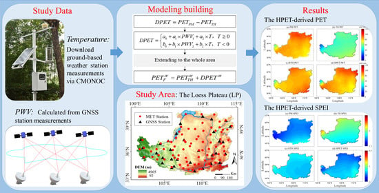
Potential evapotranspiration (PET) can reflect the characteristics of drought change in different time scales and is the key parameter for calculating the standardized precipitation evapotranspiration index (SPEI). The Thornthwaite (TH) and Penman–Monteith (PM) models are generally used to calculate PET, but the precision of PET derived from the TH model is poor, and a large number of meteorological parameters are required to evaluate the PM model. To obtain high-precision PET with fewer meteorological parameters, a high-precision PET (HPET) model is proposed to calculate PET by introducing precipitable water vapor (PWV) from Global Navigation Satellite System (GNSS) observation. The PET difference (DPET) between TH- and PM-derived PET was calculated first. Then, the relationship between the DPET and GNSS-derived PWV/temperature was analysed, and a piecewise linear regression model was calculated to fit the DPET. Finally, the HPET model was established by adding the fitted DPET to the initial PET derived from the TH model. The Loess Plateau (LP) was selected as the experiment area, and the statistical results show the satisfactory performance of the proposed HPET model. The averaged root mean square (RMS) of the HPET model over the whole LP area is 8.00 mm, whereas the values for the TH and revised TH (RTH) models are 34.25 and 12.55 mm, respectively, when the PM-derived PET is regarded as the reference. Compared with the TH and RTH models, the average improvement rates of the HPET model over the whole LP area are 77.5 and 40.5%, respectively. In addition, the HPET-derived SPEI is better than that of the TH and RTH models at different month scales, with average improvement rates of 49.8 and 23.1%, respectively, over the whole LP area. Such results show the superiority of the proposed HPET model to the existing PET models.

1. Introduction

Potential evapotranspiration (PET) reflects the rate of large-area evapotranspiration, which is an important parameter for calculating the standardized precision evapotranspiration index (SPEI) [1,2]. PET, as one of the input data of the hydrological model, is also the key to water resource assessment [3]. Therefore, retrieving PET with high precision has extensive research relevance in hydrology, agriculture, climate and other disciplines [4].

The estimation of PET can be traced to the empirical evaporation formula proposed by Dalton [5]. Bowen then put forward a new simple ratio energy balance method according to the surface energy balance equation [6], but the calculation requires that the underlying surface is uniform and has no advection effect [7]. After that, the models commonly used to calculate PET were proposed by [8,9], which are called the Thornthwaite (TH) and Penman–Monteith (PM) models, respectively. The PET value can be easily obtained using the TH model, and only the parameters of temperature and latitude are required, but the precision of the calculated PET is poor [8]. The PM model considers the effect of various meteorological factors, such as radiation, temperature, water vapor pressure and wind speed on evapotranspiration, and introduces the internal resistance of the closed crop canopy to obtain high-precision evapotranspiration data [9]; therefore, the PM-derived PET has high precision and is usually considered the reference for evaluating PET values derived from other models [10]. In addition, the Food and Agriculture Organization of the United Nations revised the PM model in 1998 and made it one of the most widely used models [11]. Previous studies have been carried out to improve the precision of PET by using multiple meteorological parameters [12,13,14]; although good results were achieved, obtaining a large number of meteorological parameters at the same time is difficult in practice. Therefore, retrieving PET with fewer meteorological parameters under the premise of ensuring accuracy becomes the research highlight.

The precipitable water vapor (PWV) derived from Global Navigation Satellite Systems (GNSSs) can be used to reflect the change of atmospheric water vapor content [15]. PET can affect the transport of atmospheric water vapor through heat and water exchange between land and the atmosphere [16]. Therefore, GNSS-derived PWV has developed rapidly in drought monitoring related to PET. The authors of [17] proposed a new index to monitor drought, which is called precipitation efficiency (PE), and found a good consistency between PE and drought. The authors of [18] used the abnormal change of GNSS-derived PWV and vertical crustal displacement to evaluate drought in Yunnan Province. The authors of [19] proved the potential of establishing an index using GNSS-derived PWV and meteorological parameters for drought and flood monitoring. Therefore, the authors of [20] established a revised TH (RTH) model using GNSS-derived PWV to retrieve PET with fewer meteorological parameters, and the improvement of the RTH model was approximately 61.6% compared with the TH model. However, the RTH model ignores the difference of the model coefficients caused by geographical location and only shares a set of model coefficients.

To improve the precision of PET using fewer meteorological parameters, this paper proposes a high-precision PET (HPET) model based on GNSS-derived PWV. This model overcomes the defects of low precision in the traditional TH model and the large number of input parameters in the PM model. This model also considers the functional relationship between PWV/temperature and PET in different geographical locations, which has never been considered before. The initial PET of the HPET model was calculated using the TH model. Then, the relationship between the PET difference (DPET) derived from the PM and TH models and PWV/T was analyzed, and a piecewise linear regression model was established. Finally, the established site function relationship was extended to the whole study area. The Loess Plateau (LP) area was selected as the experiment area, and the validation results reveal that the PET and SPEI derived from the HPET model are superior to those of the existing TH and RTH models.

2. Study Area and Data Description

2.1. Study Area

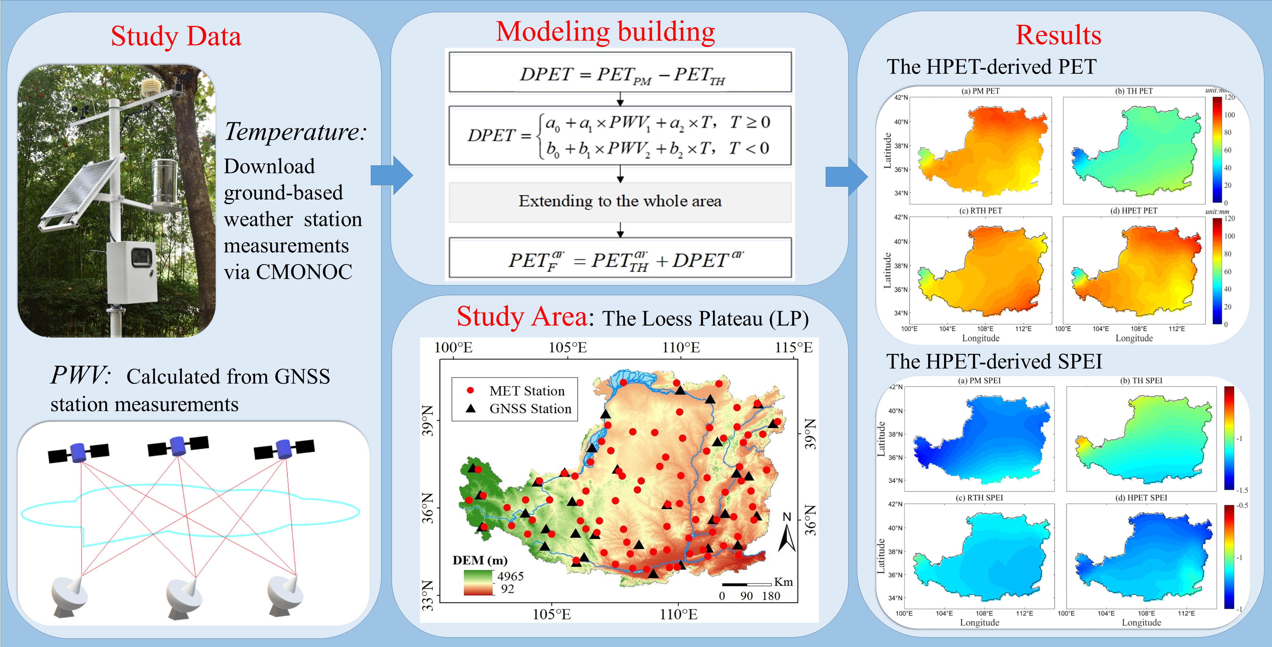
The LP is located in the north of central China, between N33°41′–41°16′ and E100°52′–114°33′. The landform in this area is undulating, with steep slopes and deep ditches, concentrated rainstorms, low vegetation coverage and a fragile ecological environment [21]. Therefore, the LP area was selected as the experiment area and 33 GNSS stations that are part of the Crustal Movement Observation Network of China (CMONOC), 84 meteorological stations operated by the China Meteorological Administration (CMA) and 4067 grid points from the fourth-generation reanalysis data (ERAI) of the European Centre for Medium-Range Weather Forecasts (ECMWF) were used to perform the experiment. Figure 1 presents the location of the LP area in China and the geographic distributions of GNSS and meteorological (MET) stations in the LP area.

2.2. Data Description

In this paper, three kinds of datasets, namely, GNSS-derived PWV, the corresponding meteorological parameters (temperature, relative humidity, etc.) and PWV provided by meteorological stations and ERAI, were selected to perform the experiment.

Table 1. Detailed information of datasets selected in this paper.

Name	Sources	Dataset	Temporal Resolution and Spatial Coverage	Counts Selected in Study	Temporal Coverage	Sources
Precipitation; Relative humidity; 2 m temperature (min, max); sunshine hours; 2 m wind speed	CMA	Daily data set of China surface climatological information (V3.0)	Daily, 824 MET stations	84 stations	2012–2018	http://data.cma.cn/ (Access data 30 February 2019)
GNSS PWV	CMONOC	\	1-hourly, 264 GNSS stations	33 stations	2012–2018	[22]
PWV; Temperature	ECMWF	ERAI	Monthly, 0.125°× 0.125°	4067 gridded points	2012–2018	http://www.ecmwf.int/ (Access data 20 July 2020)

shows the specific information of the datasets used.

The CMONOC is mainly based on the GNSS, supplemented by very long baseline interferometry, satellite laser ranging and interferometric synthetic aperture radar. The CMONOC is a national geoscience comprehensive observation network for real-time monitoring of changes in the hydrosphere and the atmosphere [23]. The CMONOC includes more than 260 continuous GNSS observation reference stations and 2000 irregular observation regional stations. In this paper, the GNSS-derived PWV from the CMONOC was used, and the root mean square (RMS) of the PWV difference between the GNSS and radiosonde is 2.25 mm for the 264 continuous GNSS stations in China. The specific procedure and validation of GNSS-derived PWV is given in detail by [22]. Thirty-three of the 264 GNSS stations were selected for the experimental area over the period 2012–2018. The elevation of the selected 33 GNSS stations ranges from 273 to 2972.1 m. In addition, all GNSS stations are equipped with the receiver of TRIMBLE NETR8, and only the double frequency observation from Global Positioning System (GPS) is used to estimate the ZTD with time resolution of 1 h.

The meteorological dataset, which includes rainfall data, wind speed, relative humidity, sunshine hours, temperature and other meteorological variables, was derived from the CMA. This dataset provides the daily data of 824 basic meteorological stations in China from 1950 to the present, which were subjected to a strict quality check. The corresponding meteorological data of 84 stations were selected in the LP area over the period 2012–2018.

ERAI is the fourth-generation reanalysis dataset of the ECMWF, which provides PWV, temperature and corresponding meteorological parameters. The highest temporal and spatial resolutions are 6 hourly and 0.125° × 0.125°, respectively. In addition, the fifth-generation reanalysis dataset of ECMWF (ERA5) replaced ERAI on 31 August 2018 with a higher temporal resolution (hourly). Due to the higher spatial resolution of ERAI compared to ERA5, the PWV and temperature data derived from ERAI over the period of 2012 to 2018 were selected in our study.

3. Theory and Methodology

3.1. Retrieval of PWV Using GNSS Observation

GNSS observation was first processed using GAMIT/GLOBK software (v10.5) [24], and zenith total delay (ZTD) and west–east directions were estimated at intervals of 1 and 2 h, respectively. The sampling rate and the elevation cut-off angle were 30s and 10°, respectively. In addition, a global mapping function was introduced [25] and the FES2004 model was also considered to obtain accurate ZTD parameters (http://holt.oso.chalmers.se/loading/, accessed on 20 July 2020). Zenith hydrological delay (ZHD) can be precisely calculated using the Saastamoinen model using surface pressure in Equation (1) [26].

$${\mathrm{ZHD}}_{SA}=\frac{0.0022768P}{1-0.00266\cos (2\phi )-0.00028H}$$

(1)

where P is the surface pressure (hPa); φ and H represents the latitude (rad) and the ellipsoid height (km) of the GNSS station, respectively. Therefore, zenith wet delay (ZWD) (m) can be obtained by subtracting ZHD (m) from ZTD (m), and PWV (mm) was finally retrieved by multiplying the conversion factor in Equation (2) [15].

$$\mathrm{PWV}=\Pi \times \mathrm{ZWD}=\frac{{10}^6}{(\frac{K_3}{T_m}+K_2^{\prime })R_V}\mathrm{ZWD}$$

(2)

where $\Pi$ is the conversion factor; R_V, $K_2^{\prime }$ and K₃ are constants with values of 461.50 (J·K⁻¹·kg⁻¹), 16.48 (K·hPa⁻¹) and 3.776 × 10⁵ (K²·hPa⁻¹), respectively; and T_m (K) is the atmospheric weighted mean temperature. In this paper, Tm was calculated based on an improved Tm model (IGPT2w), which modifies the Tm of GPT2w using gridded Tm data and ellipsoidal height grid data from the Global Geodetic Observing System in China, and the PWV error caused by the error of Tm was approximately 0.29 mm [27,28]. The GNSS-derived PWV was missing at some epochs due to instrument failure or uncorrected observation data. Singular Spectrum Analysis for Missing Data was introduced to fill the missing PWV values at those epochs, and this method has been proven effective at compensating for the missing values in a PWV time series [29].

3.2. PET Calculation Based on TH and PM Models

PET can be easily calculated based on the TH model in Equation (3), and only temperature data are used [8]. However, the deficiency of the TH model is that the PET cannot be estimated when the temperature is below zero °C [30]. In addition, the TH model only considers the effect of heat factors while ignoring the aerodynamic term; therefore, the precision of TH-derived PET (mm) is relatively poor [8].

$$\mathrm{PET}\left(\mathrm{TH}\right)=\{\begin{array}{ll}0& T\le 0\\ 16K(\frac{10T}{I}{)}^m& T>0\end{array}$$

(3)

where I and m are the heat factor and coefficient, respectively, which can be calculated by the mean monthly temperature T (°C). K is the calibrated coefficient of latitude and month.

Other than the TH model, the PM model is commonly used to obtain the high-precision PET in Equation (4). The PM model considers the effect of radiation, temperature, vapor pressure and wind speed on evapotranspiration [9].

$$\mathrm{PET}\left(\mathrm{PM}\right)=\frac{0.408\Delta (R_n-G)+\gamma \frac{900}{T+273.16}{u}_2(e_s-e_a)}{\Delta +\gamma (1+0.34u_2)}$$

(4)

where T and u₂ are the 2-m temperature (°C) and the wind speed (m·s⁻¹), respectively. e_s is the saturation vapor pressure (kPa), e_a is the actual pressure (kPa), R_n is the net radiation on the crop surface (MJ·m⁻²·d⁻¹), G is the soil heat flux (MJ·m⁻²·d⁻¹), $\Delta$ is the slope of steam pressure curve (kPa·°C⁻¹) and $\gamma$ is the humidity constant (kPa·°C⁻¹). The coefficient of the reference crop and the wind coefficient of the reference crop are 900 and 0.34, respectively. The above variables can be calculated by the daily maximum and minimum temperature, relative humidity, sunshine time and 2-m wind speed, and the specific procedure can be referenced [9].

3.3. Establishment of HPET Model

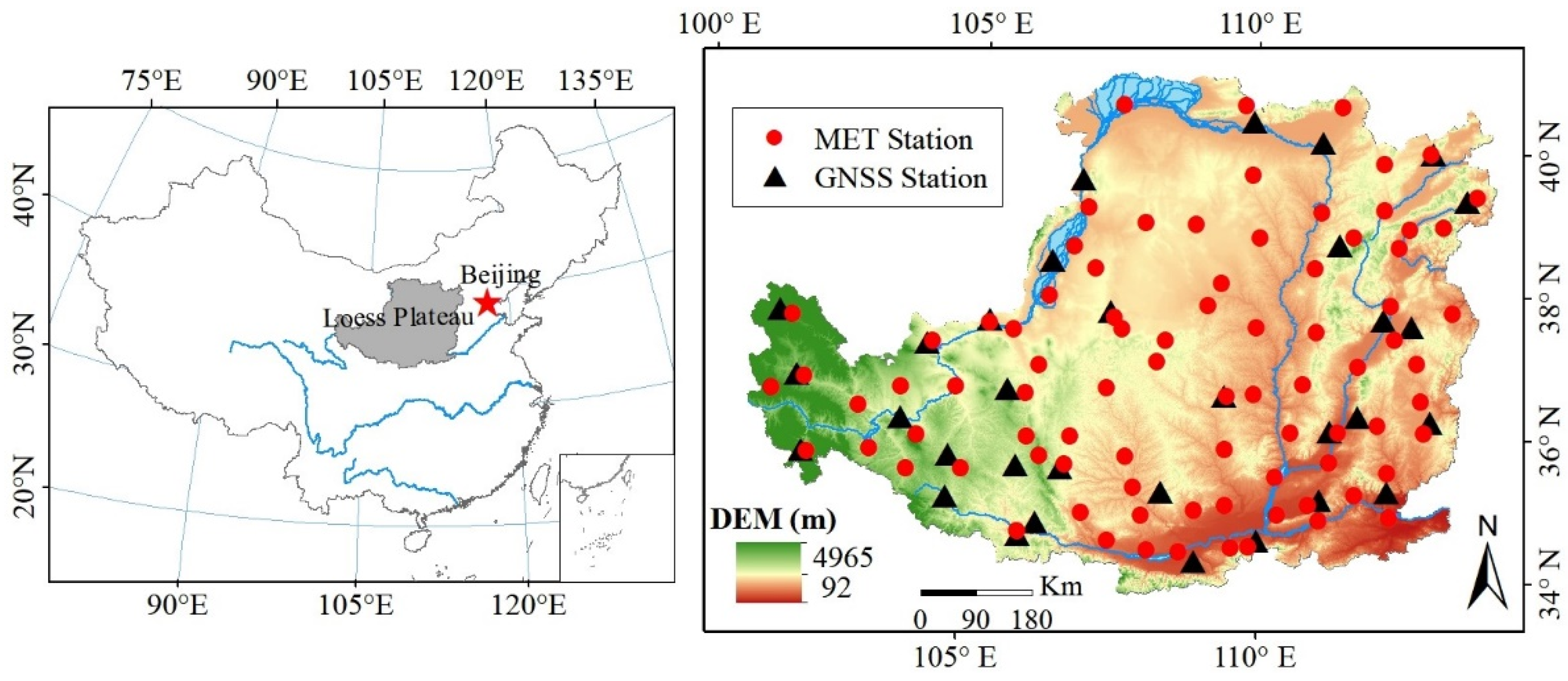
Although a high-precision PET value can be calculated using the PM model, a large number of meteorological parameters are required, which are difficult to obtain in practice. However, PET can be easily calculated using the TH model with temperature. Therefore, how to obtain a high-precision PET (HPET) by fusing the advantages of the advantages of the two models mentioned above becomes the focus of this section. The analysis of DPET in Equation (5) between the PM model and the TH model in the LP area found that the DPET values fluctuated from 24.9 to 36.2 mm. Therefore, if the TH model is used to calculate PET, the DPET should be considered to guarantee the precision of the calculated PET. According to the above analysis, this paper proposes an HPET model, and Figure 2 gives a flow chart of HPET model construction and validation. In addition, the main steps were as follows: (1) obtain the DPET difference using the TH and PM models, (2) establish the functional relationship between DPET and T/PWV, (3) extend the site-based functional relationship to the whole study area and (4) calculate the final PET value at an arbitrary location by adding the modeled DPET to the initial PET derived from the TH model.

(1)

Calculating DPET

$${\mathrm{DPET}=\mathrm{PET}}_{\mathrm{PM}}-{\mathrm{PET}}_{\mathrm{TH}}$$

(5)

(2)

Establishing the functional relationship between DPET and T/PWV

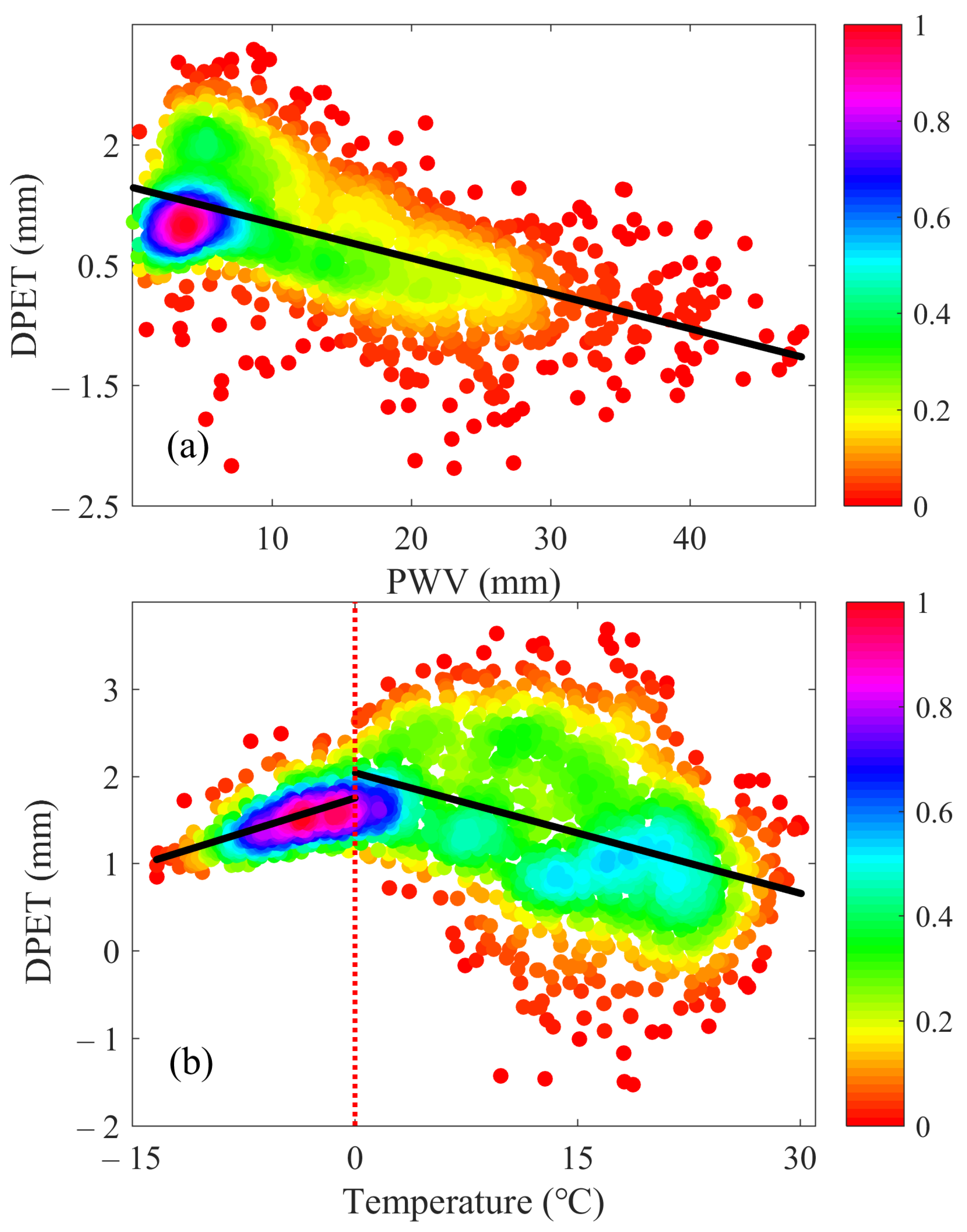
The relationship between DPET and T/PWV was first analyzed at 28 collocated sites between GNSS and meteorological stations, and Figure 3 presents the scatter diagram between DPET and T/PWV in the whole LP area over the period 2012–2018. Here, the collocated principle was that the horizontal distance is less than 0.5° between GNSS and meteorological stations, and the data utilization is larger than 85% for selected stations. In addition, the height difference between GNSS and meteorological station was also considered and the PWV correction was performed based on the empirical formula proposed in our previous work in Equation (6).

$${\mathrm{PWV}}_{h1}={\mathrm{PWV}}_{h2}·\exp (-(h1-h2)/2000)$$

(6)

where ${\mathrm{PWV}}_{h1}$ and ${\mathrm{PWV}}_{h2}$ are the PWV values at the height of $h1$ and $h2$, respectively. It could be observed that a negative linear correlation between T and DPET when T > 0 °C and a positive linear correlation between T and DPET when T < 0 °C existed. In addition, only a negative linear correlation existed between DPET and PWV, and the correlation coefficient between PWV and DPET was −0.56, and the correlation coefficient between DPET and temperature greater than 0 °C and less than 0 °C were −0.40 and 0.55, respectively, and all passed the non-zero hypothesis test (p < 0.05). Therefore, DPET can be further modelled by the piecewise linear equation using T and PWV in Equation (7).

$$\mathrm{DPET}=\{\begin{array}{c}{a}_0+a_1\times {\mathrm{PWV}}_1+a_2\times T,\hspace{1em}T\ge 0\\ b_0+b_1\times {\mathrm{PWV}}_2+b_2\times T,\hspace{1em}T<0\end{array}$$

(7)

where $a_0-a_2$ and $b_0-b_2$ are the model coefficients, which can be estimated using the least square method. PWV₁ is the PWV data at the moment of T ≥ 0 °C, PWV₂ is the PWV data at the moment of T < 0 °C.

Table 2. Model coefficients of DPET estimated at 28 collocated stations.

	Coefficient	${\mathit{a}}_0$	${\mathit{a}}_1$	${\mathit{a}}_2$	${\mathit{b}}_0$	${\mathit{b}}_1$	${\mathit{b}}_2$
Station
1		69.70	0.48	−3.88	52.64	3.01	−1.50
2		63.90	2.22	−3.86	44.65	2.90	−0.58
3		59.07	2.63	−3.75	44.57	2.07	−3.10
4		60.93	4.96	−6.77	42.83	2.60	−1.11
5		58.86	3.32	−4.81	58.93	3.01	−4.50
6		70.38	2.48	−6.22	60.55	2.81	−3.80
7		70.39	3.06	−4.92	63.06	2.78	−5.60
8		69.70	2.45	−4.31	63.09	2.62	−5.13
9		62.94	2.64	−4.27	74.40	4.39	−6.94
10		58.49	1.96	−4.03	57.61	2.56	−5.21
11		58.41	2.14	−4.02	69.95	3.53	−6.49
12		65.86	2.14	−4.52	88.49	4.02	−9.14
13		64.78	2.47	−3.80	66.94	4.07	−3.93
14		54.93	2.06	−4.21	67.49	3.36	−6.63
15		53.98	2.70	−3.20	67.35	4.32	−5.38
16		55.58	2.97	−3.47	73.79	4.67	−6.06
17		63.39	2.89	−5.28	54.44	3.16	−2.28
18		55.84	2.04	−3.06	56.76	3.61	−3.16
19		43.47	1.80	−2.17	40.75	0.49	−2.91
20		47.40	1.11	−2.65	59.97	3.50	−4.15
21		63.85	2.71	−4.15	70.55	5.78	−4.26
22		67.53	1.41	−7.06	76.73	2.88	−8.15
23		56.44	3.15	−3.76	63.98	4.29	−3.86
24		47.79	1.97	−2.11	26.22	1.65	0.92
25		50.49	1.81	−2.79	44.81	2.86	−1.83
26		46.82	3.40	−2.92	53.41	0.49	−3.96
27		49.76	1.77	−3.54	43.16	2.47	−2.15
28		67.74	0.84	−5.91	97.02	4.07	−11.84

also provides the estimated model coefficients and shows that the model coefficients fluctuated largely in the LP area, which was mainly related to the height of each GNSS station. As mentioned before, the height of GNSS stations ranged from 273 to 2973 m; therefore, the model difference caused by the geographic location of stations should be considered when establishing the DPET model, which was ignored in the previous study [20].

(3)

Extending the site-based functional relationship to the whole study area

The functional relationship between DPET and T/PWV was established at collocated stations. However, the corresponding relationship at other locations was required to obtain the DPET at the arbitrary location. Therefore, this paper introduced the multivariate quadratic polynomial to fit the model coefficients of and at the arbitrary location. The corresponding expression is as follows:

$$\left[\begin{array}{c}{a}_{01}\\ a_{02}\\ ⋮\\ a_{0n}\end{array}\right]=\left[\begin{array}{cccccccccc}1& {\phi }_1& {\lambda }_1& h_1& {\phi }_1{\lambda }_1& {\phi }_1{h}_1& {\lambda }_1{h}_1& {{\phi }_1}^2& {{\lambda }_1}^2& {h_1}^2\\ 1& {\phi }_2& {\lambda }_2& h_2& {\phi }_2{\lambda }_2& {\phi }_2{h}_2& {\lambda }_2{h}_2& {{\phi }_2}^2& {{\lambda }_2}^2& {h_2}^2\\ ⋮& ⋮& ⋮& ⋮& ⋮& ⋮& ⋮& ⋮& ⋮& ⋮\\ 1& {\phi }_n& {\lambda }_n& h_n& {\phi }_n{\lambda }_n& {\phi }_n{h}_n& {\lambda }_n{h}_n& {{\phi }_n}^2& {{\lambda }_n}^2& {h_n}^2\end{array}\right]\left[\begin{array}{c}{A}_1\\ A_2\\ ⋮\\ A_n\end{array}\right]$$

(8)

where n is equal to 28; ${\phi }_1-{\phi }_{28}$, ${\lambda }_1-{\lambda }_{28}$ and $h_1-h_{28}$ are the latitude, longitude and ellipsoid height of 28 collocated stations. $a_{0i}(i=1\cdots 28)$ are the model coefficients of 28 collocated stations, and $A_1-A_{28}$ are the fitted coefficients for model coefficients $a_{0i}$. Similarly, the other model coefficients at the arbitrary location can be estimated in Equation (8).

(4)

Calculating the final PET value

After the model coefficients of the DPET model were fitted to the whole LP area, the DPET value could be calculated at the arbitrary location. In addition, the initial PET value could be obtained using the TH model. Therefore, the final PET was obtained in Equation (9):

$${\mathrm{PET}}_F^{ar}={\mathrm{PET}}_{\mathrm{TH}}^{ar}+{\mathrm{DPET}}^{ar}$$

(9)

where ${\mathrm{PET}}_{\mathrm{TH}}^{ar}$ is the TH-derived PET, ${\mathrm{DPET}}^{ar}$ is the DPET estimated by the piecewise linear equation, and $ar$ represents the arbitrary location of the LP area.

3.4. SPEI Calculation Based on HPET Model

PET is a key parameter for SPEI calculation and can be accumulated in different time scales [31]. The differential time series between daily precipitation and PET was first calculated using Equation (10).

$$D_i=P_i-{\mathrm{PET}}_i$$

(10)

where $i$ represents the day, $D_i$ is the differenced time series and $P_i$ (mm) is the daily precipitation. Three-parameter Log-Logistic distribution was used to standardized $D_i$ to obtain the probability density function $F(x)$, which was further used to calculate SPEI in Equation (11).

$$\begin{array}{c}\mathrm{SPEI}=W-\frac{2.515517+0.802853W+0.010328W^2}{1+1.432788W+0.189269W^2+0.001308W^3}\\ W=\{\begin{array}{c}\sqrt{-2\ln (F(x))},F(x)<0.5\hfill \\ \sqrt{-2\ln (1-F(x))},F(x)>0.5\hfill \end{array}\\ F(x)={[1+{{\displaystyle \left(\frac{\alpha }{x-\lambda }\right)}}^{\beta }]}^{-1}\end{array}$$

(11)

where $\alpha$, $\beta$ and $\lambda$ are the scale parameter, shape parameter and origin parameter calculated by the L-Moment Procedure, respectively, and the detailed process is given in [32]. SPEI combines the sensitivity of partial differential equations to evapotranspiration changes with time characteristics and comprehensively considers the effect of precipitation and temperature [33]. The 1-month scale SPEI usually represents meteorological drought; the 3- to 6-month scale SPEI is considered as an agricultural drought index; the 6- to 12-month scale SPEI is used to reflect the hydrological drought and to detect the long-term evolution of surface water resources [2]. Therefore, SPEI with different time scales can identify different drought types in the context of global warming [32].

3.5. Evaluation Index of HPET Model

RMS, mean absolute error (MAE), BIAS and improvement rate (IR) in Equation (12) were introduced to evaluate the proposed HPET model.

$$\begin{array}{l}\mathrm{RMS}=\sqrt{\frac{1}{n}{\displaystyle \sum _{i=1}^n{(X_i-\overline{X})}^2}}\\ \mathrm{MAE}=\frac{1}{n}{\displaystyle \sum _{i=1}^n|(X_i-\overline{X})|}\\ \mathrm{BIAS}={\displaystyle \sum _{i=1}^n(X_i-\overline{X})/n}\\ \mathrm{IR}=\frac{{\mathrm{RMS}}_j-{\mathrm{RMS}}_{\mathrm{TH}/\mathrm{RTH}}}{{\mathrm{RMS}}_{\mathrm{TH}/\mathrm{RTH}}}\times 100\%\end{array}$$

(12)

where $X_i$ is the PET derived from the TH, RTH, or HPET models, whereas $\overline{X}$ is the PET derived from the PM model and used as the reference value. ${\mathrm{RMS}}_j$ represents the RMS of the RTH or HPET models, whereas ${\mathrm{RMS}}_{\mathrm{TH}/\mathrm{RTH}}$ is the RMS of the TH or RTH model.

4. Results of HPET Model

4.1. Calibration of ERAI-Derived PWV

The ERAI-derived PWV should be calibrated before use due to the systematic bias between the ERAI- and GNSS-derived PWV [34]. Here, the geopotential of the grid points was first converted into an ellipsoidal height according to [35]. The specific steps could be referenced. The corresponding PWV was interpolated to the collocated stations by bilinear interpolation, and the PWV error caused by the height difference between the collocated station and the grid point was corrected first [23]. Therefore, the bias between the GNSS and the ERAI at 28 collocated stations could be obtained and fitted to the whole study area using the polynomial fitting method.

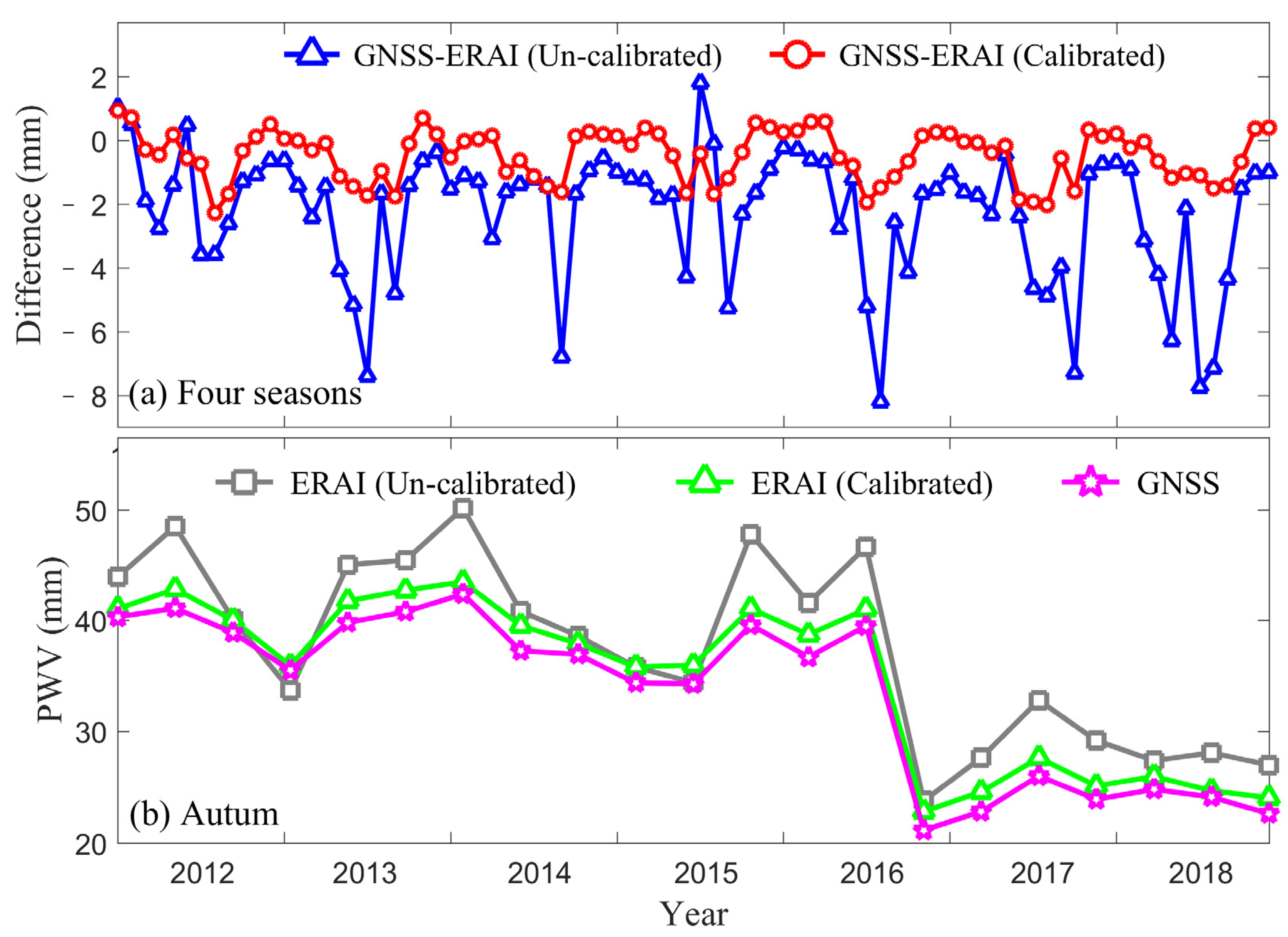
The leave one out cross-validation (LOOCV) method was used to evaluate the calibrated result because the generalization error calculated using this method has almost no deviation and can eliminate the influence of random factors [36]. In the LOOCV method, only one station was selected as the validated sample, and the 27 other stations were used for calibration. This procedure was repeated 28 times until all the stations were used as validated samples.

Table 3. Average RMS of PWV difference between GNSS-derived PWV and ERAI-derived PWV before and after calibration at 28 collocated stations over the period 2012–2018.

Season	Internal		External
	Un-Calibrated (mm)	Calibrated (mm)	Un-Calibrated (mm)	Calibrated (mm)
Spring	1.50	0.78		0.96
Summer	2.13	0.90		1.12
Fall	3.82	1.29		1.59
Winter	1.85	0.80		1.00
Ave.	2.33	0.94		1.17

provides the statistical results of the average RMS of PWV difference between the GNSS and the ERAI before and after calibration at 28 collocated stations over the period 2012–2018 in four seasons. The ERAI-derived PWV calibrated by the GNSS-derived PWV was improved in terms of the internal/external validations at four seasons. External validation refers to the fact that we used the data of 25 collocated stations to fit the PWV difference and further for fitting the PWV difference of the remaining three collocated stations. Internal validation refers to the fact that we used the data of 25 collocated stations to fit the PWV difference and further for calculating the corresponding PWV difference at those stations. The RMS of the PWV-difference-derived GNSS and ERAI is approximately 1 mm; therefore, the performance of the ERAI-derived PWV in four seasons is reasonable and acceptable. Figure 4 shows the monthly PWV difference between the ERAI and the GNSS over the whole year and the PWV series in autumn at one GNSS station (SXDT, E40.1° N113.4°) over the period 2012–2018. It can be found that the PWV difference is relatively large in the autumn before calibration. However, the ERAI-derived PWV after calibration is consistent with the GNSS-derived PWV and the PWV difference is small, which further verifies the necessity of calibrating the ERAI-derived PWV before use.

4.2. Validation of HPET-Derived PET

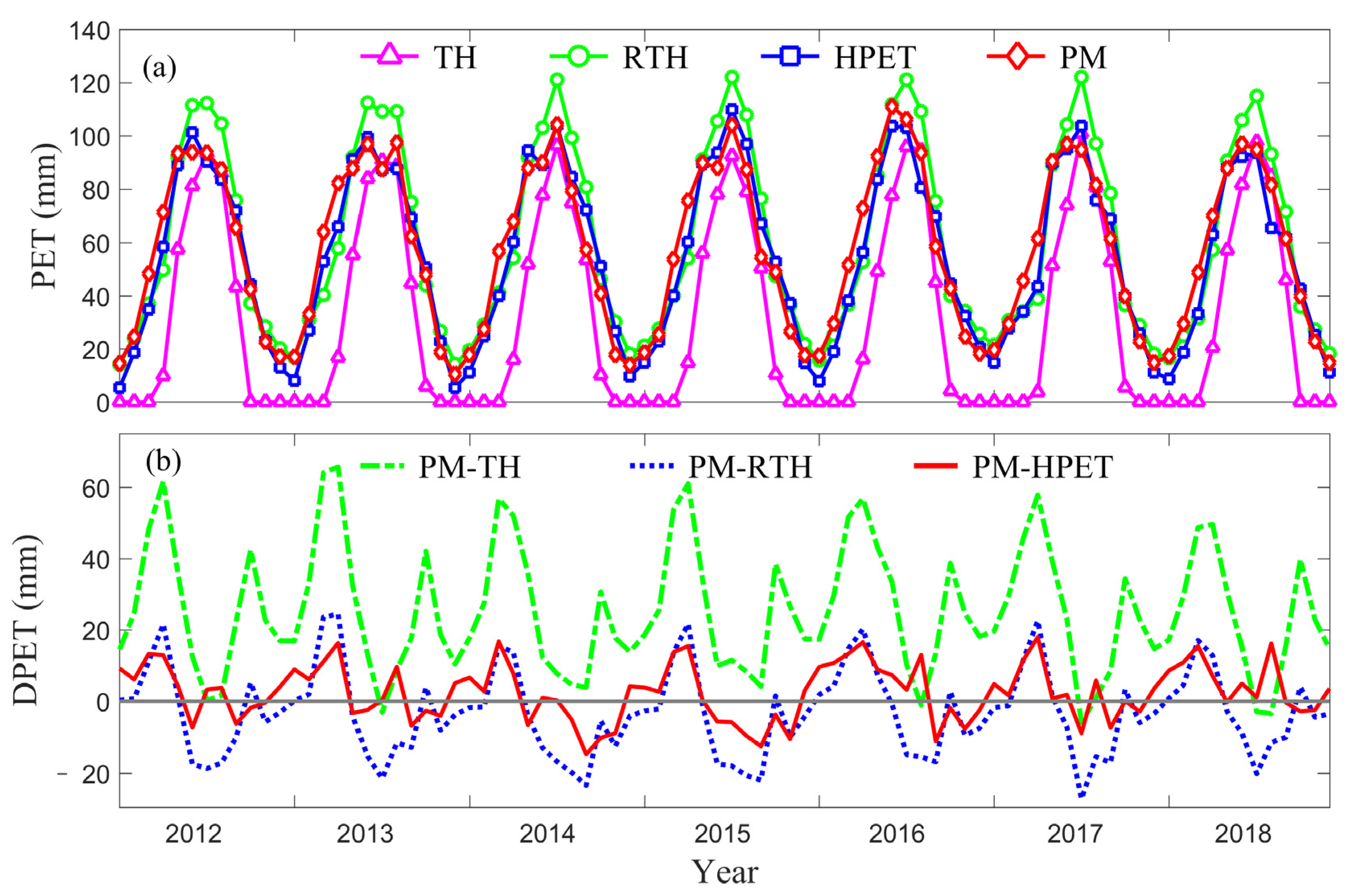
The long-term PET derived from the HPET model was first validated, and Figure 5 presents the PET derived from the PM, TH, RTH and HPET models and the PET difference between PM-TH, PM-RTH and PM-HPET at one collocated station (52,765, E37.5° N101.6°) over the period 2012–2018. It becomes obvious that TH-derived PET is underestimated for the whole period. Although the RTH-derived PET is consistent with that from the PM model when the PET value is small, the value from the RTH is overestimated when the PET value is greater than 90 mm. On the contrary, the PET estimated using the HPET model is consistent with that from the PM model over the whole period. It can also be observed that the PET difference between the PM and HPET model is the smallest over the whole period, while the fluctuations of the PET differences between PM-TH and PM-RTH are large. Therefore, the results confirm the satisfactory performance of the proposed HPET model.

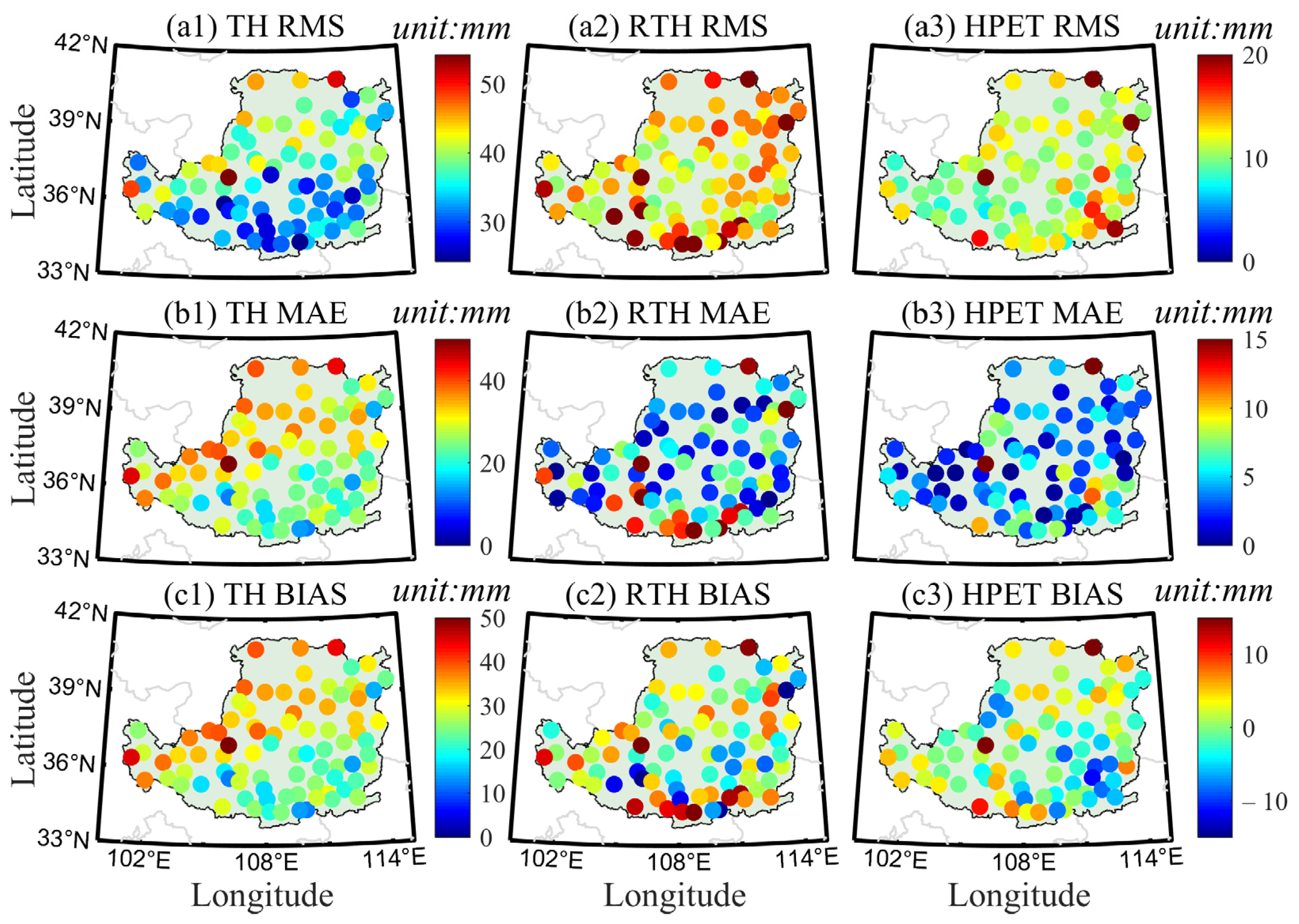
To further analyze the performance of the HPET model over the whole LP area, the RMS, MAE and BIAS of PET difference between TH/RTH/HPET and PM models at 84 meteorological stations were calculated over the period 2012–2018. Figure 6 shows the spatial distributions of the RMS, MAE and BIAS of the TH, RTH and HPET models at those meteorological stations, different scales in the color bars between TH, RTH and HPET have been used. It can be observed that the accuracy of the TH model is poor over the whole LP area compared with the RTH and HPET models. Although the spatial distribution of the RMS, MAE and BIAS of the RTH model is similar to that of the HPET model, the corresponding values of the RTH model are larger than those of the HPET model. To quantify the performance of different PET models, the average RMS, MAE, BIAS and IR of the three models were calculated with the PM-derived PET regarded as the reference at 28 GNSS stations, 84 meteorological stations and 4047 grid points of the ERAI, respectively.

Table 4. Statistical results of RMS, MAE, BIAS and IR of the TH, RTH and HPET models at GNSS, meteorological stations and grid points over the period 2012–2018.

Model	Indices	GNSS Stations	Meteorological Stations	Grid Points of ERAI	Ave.
TH	RMS (mm)	34.45	38.00	30.30	34.25
	MAE (mm)	30.05	32.80	29.09	30.65
	BIAS (mm)	27.50	28.17	29.09	28.25
	IR (%)	72.5	68.9	91.0	77.5
RTH	RMS (mm)	15.88	14.70	7.08	12.55
	MAE (mm)	12.30	11.47	5.34	9.70
	BIAS (mm)	0.00	1.15	0.36	0.50
	IR (%)	40.4	19.5	61.6	40.5
HPET	RMS (mm)	9.46	11.83	2.72	8.00
	MAE (mm)	7.55	9.67	1.92	6.38
	BIAS (mm)	0.00	0.00	0.61	0.20

provides the statistical results of the RMS, MAE, BIAS and IR of different models compared with PM at the GNSS, meteorological stations and grid points over the period 2012–2018. It can be concluded that HPET shows the highest consistency with the PM model. The RTH model is the second, and the TH model is the worst. In addition, the average IRs of the HPET model are 77.5 and 40.5%, respectively, when compared with the TH and RTH models over the whole LP area. Such results also verify the superiority of the proposed HPET model.

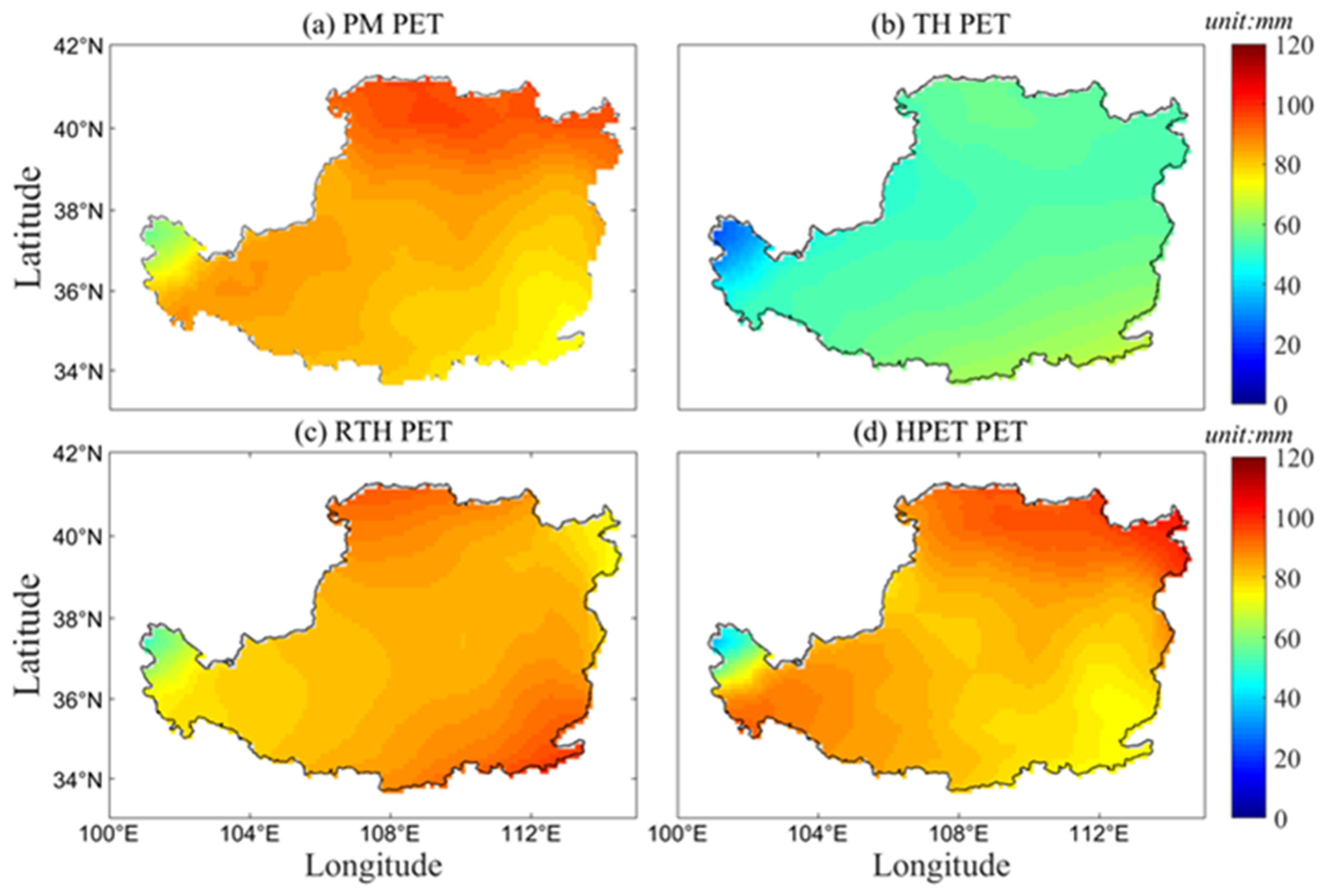
In addition, the spatial distribution of the averaged PET derived from different models over the period 2012–2018 in the LP area is presented in Figure 7. TH underestimates PET over the whole LP area. Although the RTH-derived PET has values similar to those of the PM model, the spatial distribution is not consistent with that of the PM model. However, the HPET-derived PET shows a spatial distribution similar to those of the PM model.

4.3. Validation of HPET-Derived SPEI

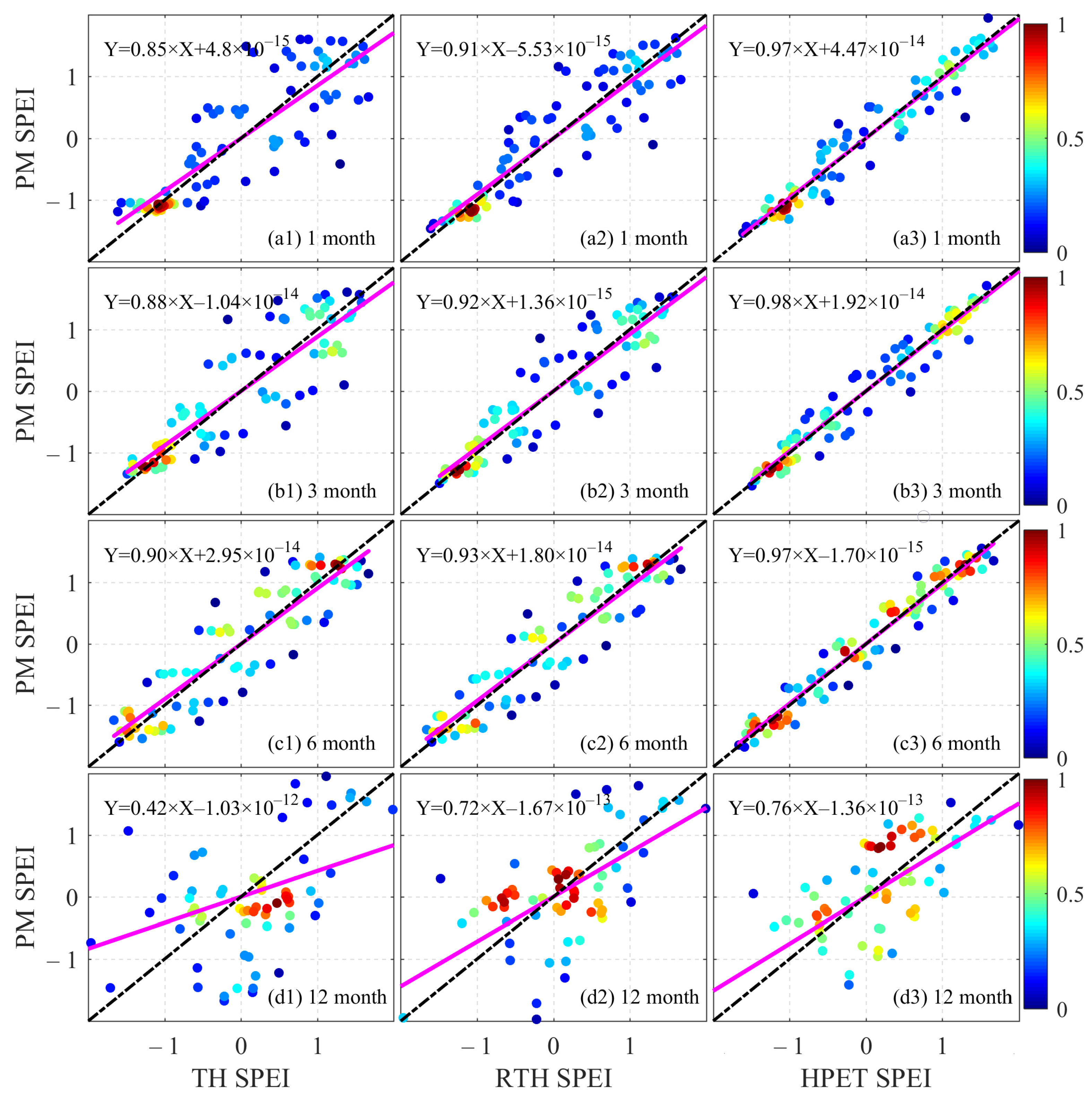
To validate the performance of the HPET-derived drought index, the SPEI using the HPET-derived PET and corresponding precipitation under different month scales was calculated. Figure 8 gives the scatter plot of the daily SPEI density at one station 52,996 (42996, 35.4°E 104.8°N) using the PET derived from the TH, RTH, HPET and PM models under the 1-, 3-, 6- and 12-month scale over the period 2012–2018 in the LP area. It can be observed that the daily SPEI calculated using the HPET-derived PET agrees well with that calculated using the means of the PM model under 1-, 3- 6- and 12- month scales. The slope of the linear fitting between the HPET and PM models is closer to one when compared with that between the TH/RTH and PM models.

Table 5. Statistical results of correlation coefficient and RMSE of SPEI between PM and different models at one station 52,996 under 1-, 3-, 6- and 12-month scales over the period 2012–2018 in the LP area.

	Model	TH		RTH		HPET
Scale		RMS	R2	RMS	R2	RMS	R2
1		0.54	0.85	0.42	0.91	0.25	0.97
3		0.49	0.88	0.39	0.92	0.22	0.98
6		0.44	0.9	0.37	0.93	0.23	0.97
12		1.07	0.42	0.74	0.72	0.69	0.76

also provides the correlation coefficient and RMSE of the SPEI difference between PM and different models under 1-, 3-, 6- and 12-month scales over the period 2012–2018 in the LP area. It can be concluded that the correlation coefficient and RMSE of the HPET-derived SPEI is superior to that of the TH and RTH models. The correlation coefficient is as high as 0.98 and the RMSE is as low as 0.22 between the PM- and HPET-derived SPEIs at a 3-month scale.

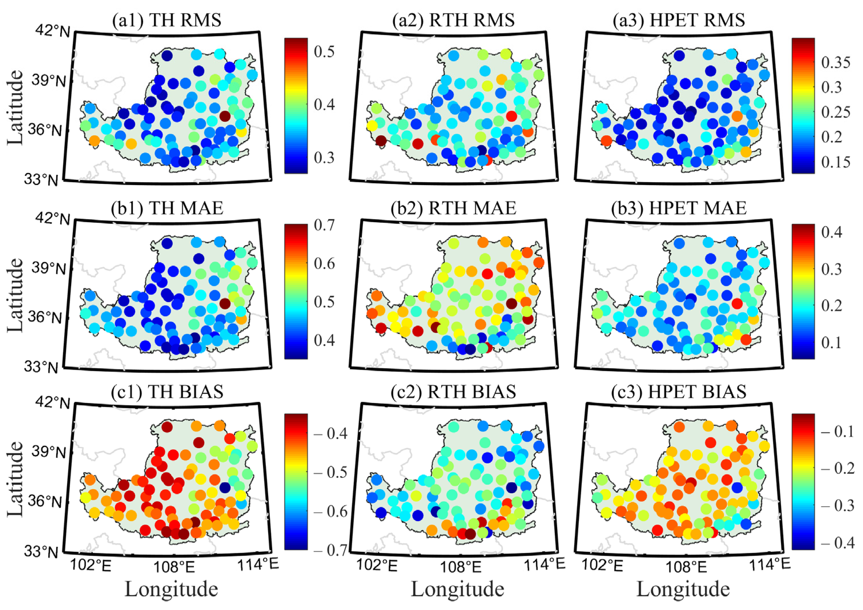
To further evaluate the performance of the proposed HPET model for calculating the SPEI, RMS, MAE, BIAS and IR of SPEI difference between the PM and different models over the whole LP area, Figure 9 shows the distributions of the RMS, MAE and BIAS of the SPEI difference derived from the PM and TH/RTH/HPET models under a 6-month scale at 84 meteorological stations over the period 2012–2018; different scales in the color bars between TH, RTH and HPET have been used. It can be observed that the RMS, MAE and BIAS of the TH model are the worst with fluctuating values of 0.25–0.55, 0.35–0.70 and −0.35–0.70, respectively, compared with the RTH and HPET models. Although the RMS, MAE and BIAS of the RTH model have the same range as the HPET model, the specific values of the RMS, MAE and BIAS of the RTH model are larger than those of the HPET model at the corresponding meteorological stations. In addition,

Table 6. Statistical results of average RMS, MAE, BIAS and IR of SPEI difference between PM and different models under 1-, 3-, 6- and 12-month scales over the period 2012–2018.

	Model	1			3			6			12
		R MS	M AE	IR (%)	R MS	M AE	IR (%)	R MS	M AE	IR (%)	R MS	M AE	IR (%)
GNSS	TH	0.47	0.38	55.3	0.57	0.49	61.4	0.57	0.50	60.0	0.31	0.26	–3.2
	RTH	0.30	0.25	30.0	0.36	0.31	38.9	0.40	0.34	37.5	0.30	0.25	–6.7
	HPET	0.21	0.17	\	0.22	0.18	\	0.25	0.20	\	0.32	0.26	\
MET.	TH	0.42	0.34	45.2	0.38	0.32	47.4	0.34	0.30	41.2	0.87	0.71	8.0
	RTH	0.26	0.21	11.5	0.24	0.20	16.6	0.24	0.20	16.7	0.78	0.65	–3.1
	HPET	0.23	0.19	\	0.20	0.16	\	0.20	0.17	\	0.80	0.67	\
ERAI	TH	0.26	0.24	76.9	0.17	0.16	5.9	0.51	0.50	54.9	1.48	1.39	35.5
	RTH	0.08	0.06	25.0	0.16	0.15	0.0	0.34	0.33	32.4	1.03	0.88	7.8
	HPET	0.06	0.05	\	0.16	0.15	\	0.23	0.22	\	0.95	0.81	\

also shows the statistical results of the averaged RMS, MAE, BIAS and IR of the SPEI difference between the PM and different models under 1-, 3-, 6- and 12-month scales over the period 2012–2018. It can be observed that the HPET-derived SPEIs at 1-, 3- and 6-month scales are superior to those of the TH and RTH models in the LP area when the PM-derived SPEI is considered as the reference. However, the performance of the obtained SPEI at a 12-month scale from different models are similar, which is mainly due to the similar accumulated error in the different models [20].

5. Conclusions

The retrieval of high-precision PET can be realized at specific stations based on the PM model, but a large number of meteorological parameters are required, which is difficult to obtain practically. Although the TH model can also be used to obtain PET using only temperature, the precision is poor. Therefore, a high-precision PET (HPET) model was proposed, which only uses temperature and the GNSS-derived PWV. In the HPET model, the TH-derived PET is considered as the initial value of the HPET model. Then, the DPET between the PM and TH models is fitted by temperature and PWV and extended to the whole study area. The LP area was selected as the experiment area, and the corresponding PWV and meteorological data from the GNSS, meteorological stations and ERAI were determined over the period 2012–2018. The numerical results showed the satisfactory performance of the proposed HPET model, and high-precision PET can be obtained with fewer meteorological parameters. Compared with the existing TH and RTH models, the accuracy of the HPET model is the highest in terms of the RMS, MAE and BIAS at the GNSS, meteorological stations and grid points, respectively. The improvement rates of the RMS of the HPET model are approximately 72.5%/40.4%, 68.9%/19.5% and 91.0%/61.6% compared with the TH and RTH models at the GNSS, meteorological stations and grid points, respectively. In addition, the HPET-derived SPEI at different month scales were also validated at the GNSS/meteorological stations and grid points, respectively, and similar results were obtained. Therefore, the proposed HPET model in this paper is superior to the existing TH and RTH models, which has great significance for the calculation of PET, the SPEI and drought studies. With the development of the GNSS, the GNSS-derived PWV can be easily obtained with high density; therefore, the proposed method in this manuscript has great potential for calculating high precision PET.

References

- Penman, H.L. Natural evaporation from open water, bare soil and grass. Proc. R. Soc. Lond. Ser. A Math. Phys. Sci. 1948, 193, 120–145. [Google Scholar]
- Beguería, S.; Vicente-Serrano, S.M.; Reig, F.; Latorre, B. Standardized precipitation evapotranspiration index (SPEI) revisited: Parameter fitting, evapotranspiration models, tools, datasets and drought monitoring. Int. J. Climatol. 2014, 34, 3001–3023. [Google Scholar] [CrossRef] [Green Version]
- Douglas, E.M.; Jacobs, J.M.; Sumner, D.M.; Ray, R.L. A comparison of models for estimating potential evapotranspiration for Florida land cover types. J. Hydrol. 2009, 373, 366–376. [Google Scholar] [CrossRef]
- Weerasinghe, I.; Bastiaanssen, W.; Mul, M.; Jia, L.; Griensven, A.V. Can we trust remote sensing evapotranspiration products over Africa. Hydrol. Earth Syst. Sci. 2020, 24, 1565–1586. [Google Scholar] [CrossRef] [Green Version]
- Experimental essays on the constitution of mixed gases; on the force of steam or vapour from water and other liquids in different temperatures, both in a Torricellian vacuum and in air; on evaporation expansion of gases by heat. Manch. Lit. Phil. Soc. Mem. Proc. 1802, 5, 536–602.
- Bowen, I.S. The ratio of heat losses by conduction and by evaporation from any water surface. Phys. Rev. 1926, 27, 779–787. [Google Scholar] [CrossRef] [Green Version]
- Kustas, W.P.; Moran, M.S.; Norman, J.M. Evaluating the spatial distribution of evaporation. In Handbook of Weather, Climate, and Water: Atmospheric Chemistry, Hydrology, and Societal Impacts; Thomas, D., Potter, B., Colman, R., Eds.; Wiley-Interscience: Hoboken, NJ, USA, 2003; pp. 461–492. [Google Scholar]
- Thornthwaite, C.W. An approach toward a rational classification of climate. Geogr. Rev. 1948, 38, 55–94. [Google Scholar] [CrossRef]
- Monteith, J.L. Evaporation and Environment. In Symposia of the Society for Experimental Biology; Cambridge University Press (CUP): Cambridge, UK, 1965; Volume 19, pp. 205–234. [Google Scholar]
- Chen, D.; Gao, G.; Xu, C.Y.; Guo, J.; Ren, G. Comparison of the Thornthwaite method and pan data with the standard Penman-Monteith estimates of reference evapotranspiration in China. Clim. Res. 2005, 28, 123–132. [Google Scholar] [CrossRef]
- Allen, R.G.; Pereira, L.S.; Howell, T.A.; Jensen, M.E. Evapotranspiration information reporting: II. Recommended documentation. Agric. Water Manag. 2011, 98, 921–929. [Google Scholar] [CrossRef]
- Wang, K.; Liang, S. An improved method for estimating global evapotranspiration based on satellite determination of surface net radiation, vegetation index, temperature, and soil moisture. J. Hydrometeorol. 2008, 9, 712–727. [Google Scholar] [CrossRef]
- Talsma, C.J.; Good, S.P.; Jimenez, C.; Martens, B.; Fisher, J.B.; Miralles, D.G.; McCabe, M.F.; Purdy, A.J. Partitioning of evapotranspiration in remote sensing-based models. Agric. For. Meteorol. 2018, 260, 131–143. [Google Scholar] [CrossRef]
- Chen, J.M.; Liu, J. Evolution of evapotranspiration models using thermal and shortwave remote sensing data. Remote. Sens. Environ. 2020, 237, 111594. [Google Scholar] [CrossRef]
- Bevis, M.; Businger, S.; Herring, T.A.; Rocken, C.; Anthes, R.A.; Ware, R.H. GPS meteorology: Remote sensing of atmospheric water vapor using the Global Positioning System. J. Geophys. Res. Atmos. 1992, 97, 15787–15801. [Google Scholar] [CrossRef]
- Yeh, P.J.F.; Famiglietti, J.S. Regional terrestrial water storage change and evapotranspiration from terrestrial and atmospheric water balance computations. J. Geophys. Res. Atmos. 2008, 1–13. [Google Scholar] [CrossRef]
- Bordi, I.; Raziei, T.; Pereira, L.S.; Sutera, A. Ground-based GPS measurements of precipitable water vapor and their usefulness for hydrological applications. Water Resour. Manag. 2015, 29, 471–486. [Google Scholar] [CrossRef]
- Jiang, W.; Yuan, P.; Chen, H.; Cai, J.; Li, Z.; Chao, N.; Sneeuw, N. Annual variations of monsoon and drought detected by GPS: A case study in Yunnan, China. Sci. Rep. 2017, 7, 1–10. [Google Scholar] [CrossRef]
- Wang, X.; Zhang, K.; Wu, S.; Li, Z.; Cheng, Y.; Li, L.; Yuan, H. The correlation between GNSS-derived precipitable water vapor and sea surface temperature and its responses to El Niño–Southern Oscillation. Remote. Sens. Environ. 2018, 216, 1–12. [Google Scholar] [CrossRef]
- Zhao, Q.; Ma, X.; Yao, W.; Liu, Y.; Du, Z.; Yang, P.; Yao, Y. Improved drought monitoring index using GNSS-derived precipitable water vapor over the loess plateau area. Sensors 2019, 19, 5566. [Google Scholar] [CrossRef] [Green Version]
- Gao, H.; Li, Z.; Jia, L.; Li, P.; Xu, G.; Ren, Z.; Pang, G.; Zhao, B. Capacity of soil loss control in the Loess Plateau based on soil erosion control degree. J. Geogr. Sci. 2016, 26, 457–472. [Google Scholar] [CrossRef] [Green Version]
- Zhao, Q.; Yang, P.; Yao, W.; Yao, Y. Hourly PWV dataset derived from GNSS observations in China. Sensors 2020, 20, 231. [Google Scholar] [CrossRef] [Green Version]
- Zhang, W.; Lou, Y.; Huang, J.; Zheng, F.; Cao, Y.; Liang, H.; Shi, C.; Liu, J. Multiscale variations of precipitable water over China based on 1999–2015 ground-based GPS observations and evaluations of reanalysis products. J. Clim. 2018, 31, 945–962. [Google Scholar] [CrossRef]
- Herring, T.A.; King, R.W.; McClusky, S.C. GAMIT Reference Manual, GPS Analysis at MIT. 2010. Available online: http://www-gpsg.mit.edu/~simon/gtgk/index.htm (accessed on 8 August 2020).
- Böhm, J.; Niell, A.; Tregoning, P.; Schuh, H. Global Mapping Function (GMF): A new empirical mapping function based on numerical weather model data. Geophys. Res. Lett. 2006, 36–45. [Google Scholar] [CrossRef] [Green Version]
- Saastamoinen, J. Atmospheric correction for the troposphere and stratosphere in radio ranging satellites. Use Artif. Satell. Geod. 1972, 15, 247–251. [Google Scholar]
- Böhm, J.; Möller, G.; Schindelegger, M.; Pain, G.; Weber, R. Development of an improved empirical model for slant delays in the troposphere (GPT2w). GPS Solut. 2015, 19, 433–441. [Google Scholar] [CrossRef] [Green Version]
- Huang, L.; Liu, L.; Chen, H.; Jiang, W. An improved atmospheric weighted mean temperature model and its impact on GNSS precipitable water vapor estimates for China. GPS Solut. 2019, 23, 1–16. [Google Scholar] [CrossRef]
- Wang, X.; Cheng, Y.; Wu, S.; Zhang, K. An effective toolkit for the interpolation and gross error detection of GPS time series. Surv. Rev. 2016, 48, 202–211. [Google Scholar] [CrossRef]
- Sheffield, J.; Wood, E.F.; Roderick, M.L. Little change in global drought over the past 60 years. Nature 2012, 491, 435–438. [Google Scholar] [CrossRef]
- Potop, V.; Možný, M. The application a new drought index–Standardized precipitation evapotranspiration index in the Czech Republic. Mikroklima Mezoklima Kraj. Struct. Antropog. Prostředí 2011, 2, 1–12. [Google Scholar]
- Vicente-Serrano, S.M.; Beguería, S.; López-Moreno, J.I. A multiscalar drought index sensitive to global warming: The standardized precipitation evapotranspiration index. J. Clim. 2010, 23, 1696–1718. [Google Scholar] [CrossRef] [Green Version]
- Li, X.; He, B.; Quan, X.; Liao, Z.; Bai, X. Use of the standardized precipitation evapotranspiration index (SPEI) to characterize the drying trend in southwest China from 1982–2012. Remote Sens. 2015, 7, 10917–10937. [Google Scholar] [CrossRef] [Green Version]
- Zhang, B.; Yao, Y. Precipitable water vapor fusion based on a generalized regression neural network. J. Geod. 2021, 95, 1–14. [Google Scholar] [CrossRef]
- Wang, X.; Zhang, K.; Wu, S.; Fan, S.; Cheng, Y. Water vapor-weighted mean temperature and its impact on the determination of precipitable water vapor and its linear trend. J. Geophys. Res. Atmos. 2016, 121, 833–852. [Google Scholar] [CrossRef]
- Liu, J.; Huffman, T.; Qian, B.; Shang, J.; Li, Q.; Dong, T.; Davidson, A.; Jing, Q. Crop yield estimation in the Canadian prairies using Terra/MODIS-derived crop metrics. IEEE J. Sel. Top. Appl. Earth Obs. Remote Sens. 2020, 13, 2685–2697. [Google Scholar] [CrossRef]
Figure 1.
Location of the LP in China and the geographic distributions of GNSS and meteorological (MET) stations in the LP area.
Figure 2.
Flow chart of HPET model construction and validation.
Figure 3.
Scatter diagram between daily (a) DPET and T, as well as (b) DPET and PWV in the whole LP area over the period 2012–2018. The color represents the density of the dots.
Figure 4.
PWV difference between ERAI and GNSS (a) in the whole year and (b) the monthly PWV long time in fall at one GNSS station (SXDT, E40.1° N113.4°) over the period 2012–2018.
Figure 5.
Comparison of (a) PET derived from the PM, TH, RTH and HPET models and (b) PET difference between PM-TH, PM-RTH and PM-HPET models at one collocated station (52,765, E37.5° N101.6°) over the period 2012–2018.
Figure 6.
Spatial distributions of (a1) RMS of TH model, (a2) RMS of RTH model, (a3) RMS of HPET model, (b1) MAE of TH model, (b2) MAE of RTH model, (b3) MAE of HPET model, (c1) BIAS of TH model, (c2) BIAS of RTH model and (c3) BIAS of HPET model at meteorological stations over the LP area.
Figure 7.
Spatial distribution of average PET derived from (a) PM model, (b) TH model, (c) RTH model and (d) HPET model over the period 2012–2018 in the LP area.
Figure 8.
Scatter plot of daily SPEI density at one station using PET derived from (a1) TH-PM model, (a2) RTH-PM model, (a3) HPET-PM model under 1-month scale, (b1) TH-PM model, (b2) RTH-PM model, (b3) HPET-PM model under 3-month scale, (c1) TH-PM model, (c2) RTH-PM model, (c3) HPET-PM model under 6-month scale, (d1) TH-PM model, (d2) RTH-PM model, (d3) HPET-PM model under 12-month scale, respectively over the period 2012–2018 in the LP area. The color represents the density of the dots.
Figure 9.
Spatial distributions of (a1) RMS of TH model, (a2) RMS of RTH model, (a3) RMS of HPET model, (b1) MAE of TH model, (b2) MAE of RTH model, (b3) MAE of HPET model, (c1) BIAS of TH model, (c2) BIAS of RTH model, (c3) BIAS of HPET model, respectively under a 6-month scale at 84 meteorological stations over the period 2012–2018.