
Exploring Fuzzy Local Spatial Information Algorithms for Remote Sensing Image Classification


1
International Institute of Spatial Lifecourse Epidemiology (ISLE), Wuhan University, Wuhan 430072, China
2
Indian Institute of Remote Sensing, ISRO, 4 Kalidas Road, Dehradun 248001, India
3
Faculty of Geo-Information Science and Earth Observation (ITC), University of Twente, 7500 AE Enschede, The Netherlands
4
School of Resources and Environmental Science, Wuhan University, Wuhan 430072, China
*
Author to whom correspondence should be addressed.
Remote Sens. 2021, 13(20), 4163; https://doi.org/10.3390/rs13204163
Submission received: 19 July 2021
/
Revised: 20 August 2021
/
Accepted: 23 August 2021
/
Published: 18 October 2021
(This article belongs to the Special Issue Advances in Optical Remote Sensing Image Processing and Applications)
Abstract
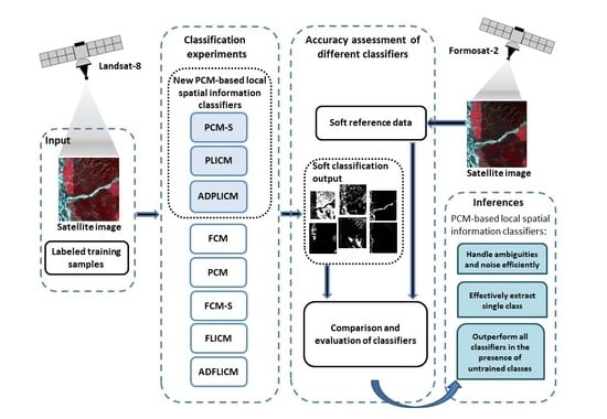
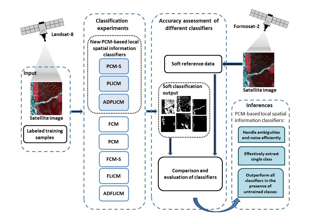
:Fuzzy c-means (FCM) and possibilistic c-means (PCM) are two commonly used fuzzy clustering algorithms for extracting land use land cover (LULC) information from satellite images. However, these algorithms use only spectral or grey-level information of pixels for clustering and ignore their spatial correlation. Different variants of the FCM algorithm have emerged recently that utilize local spatial information in addition to spectral information for clustering. Such algorithms are seen to generate clustering outputs that are more enhanced than the classical spectral-based FCM algorithm. Nonetheless, the scope of integrating spatial contextual information with the conventional PCM algorithm, which has several advantages over the FCM algorithm for supervised classification, has not been explored much. This study proposed integrating local spatial information with the PCM algorithm using simpler but proven approaches from available FCM-based local spatial information algorithms. The three new PCM-based local spatial information algorithms: Possibilistic c-means with spatial constraints (PCM-S), possibilistic local information c-means (PLICM), and adaptive possibilistic local information c-means (ADPLICM) algorithms, were developed corresponding to the available fuzzy c-means with spatial constraints (FCM-S), fuzzy local information c-means (FLICM), and adaptive fuzzy local information c-means (ADFLICM) algorithms. Experiments were conducted to analyze and compare the FCM and PCM classifier variants for supervised LULC classifications in soft (fuzzy) mode. The quantitative assessment of the soft classification results from fuzzy error matrix (FERM) and root mean square error (RMSE) suggested that the new PCM-based local spatial information classifiers produced higher accuracies than the PCM, FCM, or its local spatial variants, in the presence of untrained classes and noise. The promising results from PCM-based local spatial information classifiers suggest that the PCM algorithm, which is known to be naturally robust to noise, when integrated with local spatial information, has the potential to result in more efficient classifiers capable of better handling ambiguities caused by spectral confusions in landscapes.
1. Introduction
Land use/land cover (LULC) maps are the most useful product derived from remote sensing, as this information is vital for other applications, such as assessment and monitoring of vegetation types, crop and yield estimation, environmental impact assessment, natural resource management and monitoring, urban planning. Scientists are continually coming up with advanced classification techniques with improved classification accuracy to generate precise LULC maps. A particular classifier may not work best for all situations, as the characteristics of each image and the circumstances of each study vary greatly. For that reason, an appropriate classifier should be selected by the analyst for the task at hand [1].
Most classifiers used for satellite image analysis are based on the per-pixel approach. With conventional per-pixel classifiers or hard classifiers, the study area is assumed to consist of distinct and discrete LULC classes, which are internally homogenous [2]. The image pixels that represent geographic information on the ground are associated with a single land use or land cover class. However, a single pixel may correspond to more than one land cover in reality, such as a soil pixel with sparse grassland, which can be classified as either “grassland” or “soil” [3]. Such mixed pixels, which show affinity to more than one information class, may also occur at the indistinct class boundaries. Furthermore, ambiguities may arise due to variability within land cover classes and variation in spectral responses recorded by the sensors with corresponding ground situations. The uncertainty or fuzziness in geographic representation due to class mixtures, intermediate conditions, or within-class variability is better represented by soft classification or sub-pixel methods.
Sub-pixel scale analysis assumes an individual pixel’s spectral value to be a combination of spectral values of pure pixels from classes, i.e., the pixels are assumed to be mixed pixels. The sub-pixel scale thematic information is usually represented by soft classification outputs where the areal class proportion of each pixel is displayed, and hence a set of output fraction images is generated, one per class [4]. Such methods provide more accurate geographic representation and more truthful results, especially in the case of coarser datasets [5]. Various methods have been explored to derive soft classification outputs, a few of which are the approaches based on fuzzy-set theory, Dempster–Shafer theory, certainty factor, the softening of hard classifier outputs, neural networks, regression modeling, etc. [5,6]. Fuzzy-set-based approaches and spectral mixture analysis are the popular, simpler techniques for dealing with the mixed-pixel problem in remote sensing image classification [5]. Fuzzy set theory [7] introduced the idea of partial membership of data points in multiple clusters characterized by membership functions. The class membership values of a pixel in fuzzy-based classifiers indicate the sub-pixel scale fractional class compositions of that pixel.
One common issue in the standard unmixing or fuzzy-based soft classification methods is the requirement of defining all the classes (endmembers) [8]. As a result of this, the soft classification outputs generated from these methods depict relative measures of class membership of pixels as opposed to the absolute strength of class membership. Fuzzy c-means (FCM) [9,10], originally an unsupervised fuzzy clustering algorithm, has been successfully implemented and widely used in the field of remote sensing, both for unsupervised and supervised classifications [2,11,12,13,14,15,16]. However, FCM generates relative class membership of pixels, which means the membership of a pixel (or a data point) in a cluster is dependent on its membership in all remaining clusters [17]. Krishnapuram and Keller [18] observed the performance of FCM and its derivatives to be compromised in noisy environments because of the probabilistic constraint, which forces the membership values in FCM to be relative, and hence presented a possibilistic approach to clustering in the possibilistic c-means (PCM) algorithm. PCM is an iterative clustering algorithm similar to the FCM, but the membership of a data point (pixel) in a cluster is independent of its membership in other clusters. The membership in the PCM algorithm, therefore, represents the “degree of belonging or compatibility” as opposed to the “degree of sharing” in FCM [18]. PCM is naturally immune to noise and outliers because the noise pixels will have a low degree of compatibility in all clusters. Foody [17] suggested that PCM is more appropriate for supervised LULC classification, as untrained classes are generally encountered during supervised classification. While FCM generates the most accurate class compositions when all the classes are defined, its performance degrades in the presence of untrained classes. PCM is not affected by the presence of untrained classes and thus outperforms FCM in such scenarios [17]. Ibrahim et al. [16], on evaluating the performance of the maximum likelihood classifier (MLC), FCM, and PCM for supervised classification, found PCM to produce the highest accurate land cover maps when uncertainty existed in the dataset.
The fuzzy clustering algorithms FCM and PCM do not accommodate the spatial dependence of pixels in the input satellite image for classification [19]. The use of spectral information alone for classification often generates classification outputs that look noisy (salt and pepper effect) [20]. This is caused due to the diversity of spectral variability, inherent ground complexities, or inadequate spatial resolution [21]. Medium resolution satellite sensors, such as Landsat Thematic Mapper, cover a large area and produce images in which “the pixel size is smaller than the general extent of landscape objects” [22]. Thus, pixels within images “exhibit a high degree of spatial autocorrelation” [22], which means the pixels that are close together or that are within the local neighborhood are likely to belong to the same information class. The suitable use of this spatial information along with spectral information could help to eliminate ambiguities caused due to spectral confusions in LULC classes (intra-class spectral variation and inter-class spectral similarity), to recover the missing information, and to correct erroneous pixel classifications [5,23].
Spatial context in remote sensing image analysis can be characterized by texture extraction, filtering methods, mathematical morphology, spatial statistics, contextual techniques (segmentation and object-based image analysis), Markov random fields (MRF), relaxation labeling, the fusion of multisource data/techniques, etc. [5,6,22,24,25,26,27]. Numerous models have come up, which fuses multiple data/methods for taking full advantage of the spatial knowledge in the images for improvising the classification efficiency. Pixel-level image fusion approaches, generally categorized into multi-scale decomposition and sparse representations, are widely applied fusion approaches in remote sensing [28,29]. Anand et al. [30] used a 3D-DWT (discrete wavelet transform) for feature extraction from hyperspectral data and fed the extracted features to three machine learning (ML) algorithms, Random Forest (RF), Support Vector Machine (SVM), and K-Nearest neighbor (KNN), for classification. 3D-DWT, a multi-scale decomposition approach, incorporates the association of neighboring pixels for extracting discriminatory features while minimizing the noise in the input hyperspectral image (HSI) data. The three ML algorithms with the added 3D-DWT features performed better than the corresponding traditional version of the algorithms. Miao and Shi [20] proposed a multistep spectral-spatial method for HSI and multispectral image classification. This classification method utilized the fusion of statistical region merging (SRM) outputs and pixel-based SVM outputs using majority voting to obtain the spectral-spatial classifications.
Spatial contextual information is commonly incorporated in the spectral-based classification as pre-classification/post-classification steps or as additional feature bands during classification without modifying the classifiers. The per-pixel classifiers (SVM, RF) and subpixel classifiers (FCM) are also seen to be integrated with approaches, such as MRF and relaxation labeling, and others to simultaneously exploit the spatial and spectral information during classification [31,32,33,34]. The concept of local (neighborhood) spatial autocorrelation has emerged recently to integrate spatial information with conventional spectral-based per-pixel or sub-pixel classifiers [6,35,36]. Zhang et al. [35] modified and integrated the k-means algorithm with a neighborhood constrained index to generate a neighborhood-constrained k-means (NC-k-means) algorithm. Deng and Wu [36] came up with a spatially adaptive spectral mixture analysis (SASMA), which involved the integration of spatial and spectral information, unlike the conventional spectral mixture analysis (SMA). All the above spectral classifiers showed improved classification performance when integrated with spatial contextual information.
Deep learning approaches, especially the convolutional neural networks (CNN), have recently gained popularity because of their ability to exploit spatial data through convolution operation for feature extraction, segmentation, object detection, classification, etc. However, the 3D CNN that extracts both spectral and spatial information has high computational complexity. Hence, 2D CNNs are generally widely employed to extract spatial features (e.g., textures) from images [37]. Several studies have combined the benefits of fuzzy classification approaches with that of CNN. Balakrishnan et al. [38] proposed a meticulous fuzzy convolution c-means (MFCCM) algorithm that integrated a fuzzy clustering algorithm with CNN. Although the MFCCM algorithm utilized the significant features extracted from convolutional filtering to generate promising fuzzy clustering results in noisy environments, the algorithm exhibited limitations in terms of time complexity. Wang et al. [39] proposed a semi-supervised approach combining an improved FCM algorithm (IFCM), which effectively utilized labeled data integrated into traditional FCM for clustering, and CNN for fault detection in the sparsity of labeled data. The CNN model in this method, trained using the original data corresponding to the output labeled data from IFCM, was further used for fault detection. Although deep learning models are effective in handling complex classification scenarios by incorporating advanced learning mechanisms, large training data is required to train them to produce generalized outcomes.
The most common and simplest approach to integrating local spatial information into conventional FCM is by modifying the FCM objective function to include spatial information from the neighboring pixels within a local window. The advantage of such a method is that the spatial information can be straightforwardly incorporated into the FCM with minimum changes in the resulting implementation [19]. Integrating spatial-contextual information with spectral information in FCM has been seen to improve its robustness and classification accuracy [19,21,40,41,42,43,44,45,46]. Pham and Prince [45] came up with an iterative adaptive FCM (AFCM) algorithm that included a multiplier field term to model the brightness variations caused due to intensity inhomogeneities in magnetic resonance images. Liew et al. [46] experimented with modifying the FCM objective function with a new adaptive dissimilarity index that takes into account the influence of neighboring pixels on the central pixel within the 3 × 3 window around the pixel. Another study by Pham [19] introduced a spatial penalty term in the objective function of FCM to constrain the behavior of membership functions, keeping the centroid computations of FCM unchanged in this approach. Ahmed et al. [42], in the FCM-S algorithm, introduced a spatial neighborhood term into the conventional FCM algorithm that forced the labeling of the neighboring pixels to influence the labeling of each pixel. One limitation of this algorithm, an increase in computation time, was overcome in FCM_S1 and FCM_S2 proposed by S. Chen and Zhang [43]. FCM_S1 and FCM_S2 used a mean filter and a median filter, respectively, to simplify the computation complexity. However, the output performances of FCM-S, FCM-S1, and FCM-S2 algorithms depended on an empirically selected parameter, which controlled the robustness to noise and the effectiveness of preserving the image details. Krinidis and Chatzis [44] proposed a fuzzy local information c-means (FLICM) algorithm in which a new fuzzy factor, independent of any empirically selected parameter, was introduced into the FCM objective function. The FLICM algorithm was observed to be weak in identifying class boundary pixels and edge pixels as a result of over-smoothing [21,47]. H. Zhang et al. [21] introduced a fuzzy similarity measure based on a spatial attraction model in their adaptive fuzzy local information c-means algorithm (ADFLICM). The fuzzy similarity measure allowed each pixel during classification to be influenced by its neighboring pixels as well as its own features, thereby ensuring edge retention and noise insensitivity simultaneously. Mishra et al. [48] applied an improved FLICM algorithm as a segmentation method to extract features that were subsequently fed into the local linear wavelet neural network (LLWNN-SCA) model for breast cancer detection and classification. Suman et al. [49] performed a comparative analysis of fuzzy local spatial information algorithms, FCM-S, FLICM, and ADFLICM, with different distance measures and weighing factors.
Although the PCM algorithm is not as researched as FCM, numerous modified versions of PCM have come up recently to improve the clustering/classification performance of the conventional PCM algorithm to suit different applications [50,51,52,53,54,55,56]. In separate studies carried out by Ravindraiah and Chandra Mohan Reddy [55] and Chawla [56], the PCM algorithm was adapted to include spatial contextual information with spectral information for clustering/classification. Ravindraiah and Chandra Mohan Reddy [55] modified the PCM algorithm with induced spatial constraint to develop a spatial possibilistic c-means clustering algorithm (SPCM) for fundus image classification for diabetic retinopathy (DR) lesions. Chawla [56] developed contextual fuzzy classification algorithms using MRF with PCM as the base classifier. While the contextual PCM classifier with MRF standard regularization and the contextual PCM classifier with MRF discontinuity adaptive (DA) prior outperformed the conventional PCM classifier in terms of accuracy, the contextual PCM with DA prior preserved edges better.
The promising results of the local spatial information algorithms, FCM-S, FLICM, and ADFLICM, and the advantages of PCM over FCM in the presence of untrained classes [17], encouraged us to integrate local spatial information with the standard PCM algorithm and to investigate these algorithms for supervised LULC classification in soft (fuzzy) mode. The possibilistic c-means with spatial constraints (PCM-S), possibilistic local information c-means (PLICM), and adaptive possibilistic local information c-means (ADPLICM) algorithms are proposed, exploiting the methods used for incorporating local spatial information into the FCM-S, FLICM, and ADFLICM algorithms, respectively. The realization of the above-mentioned approaches involves simple modifications to the PCM objective function to integrate spatial data straightforwardly. With appropriate parameter values, the PCM algorithm has been proven to improve the results of FCM [57] and is recommended. Thus, we incorporate local spatial information into PCM with a view of generating better classifiers that could be used instead of, or in addition to, the FCM-based local spatial information classifiers, FCM, or PCM classifiers. The study aims not only to incorporate local spatial information into the PCM algorithm but to evaluate and compare the performance of available FCM-based local spatial information algorithms and the new PCM-based local spatial information algorithms. The contribution of our study lies in (1) understanding the potential of integrating the PCM algorithm with local spatial information for better handling of isolated pixels (noise) and other ambiguities caused by spectral confusions and (2) understanding the relevance of the choice of the fuzzy local spatial information classifiers and their parameter values, in managing outliners and generating accurate classification outputs, based on the number and nature of land cover classes for classification.
2. Materials and Methods
2.1. Study Area and Datasets
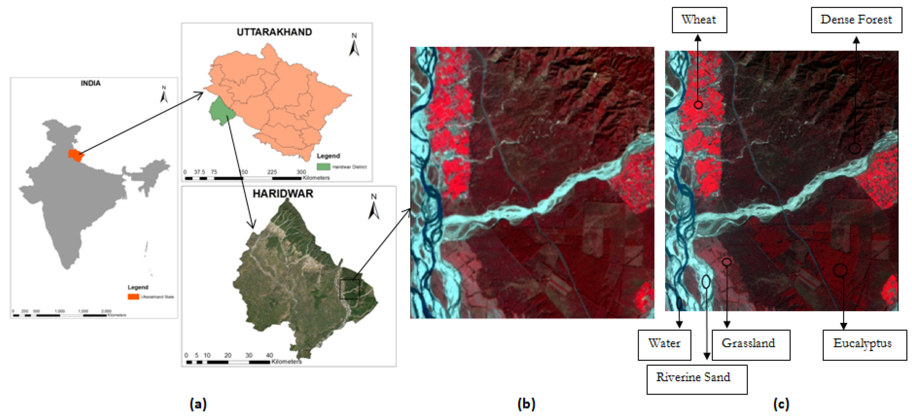
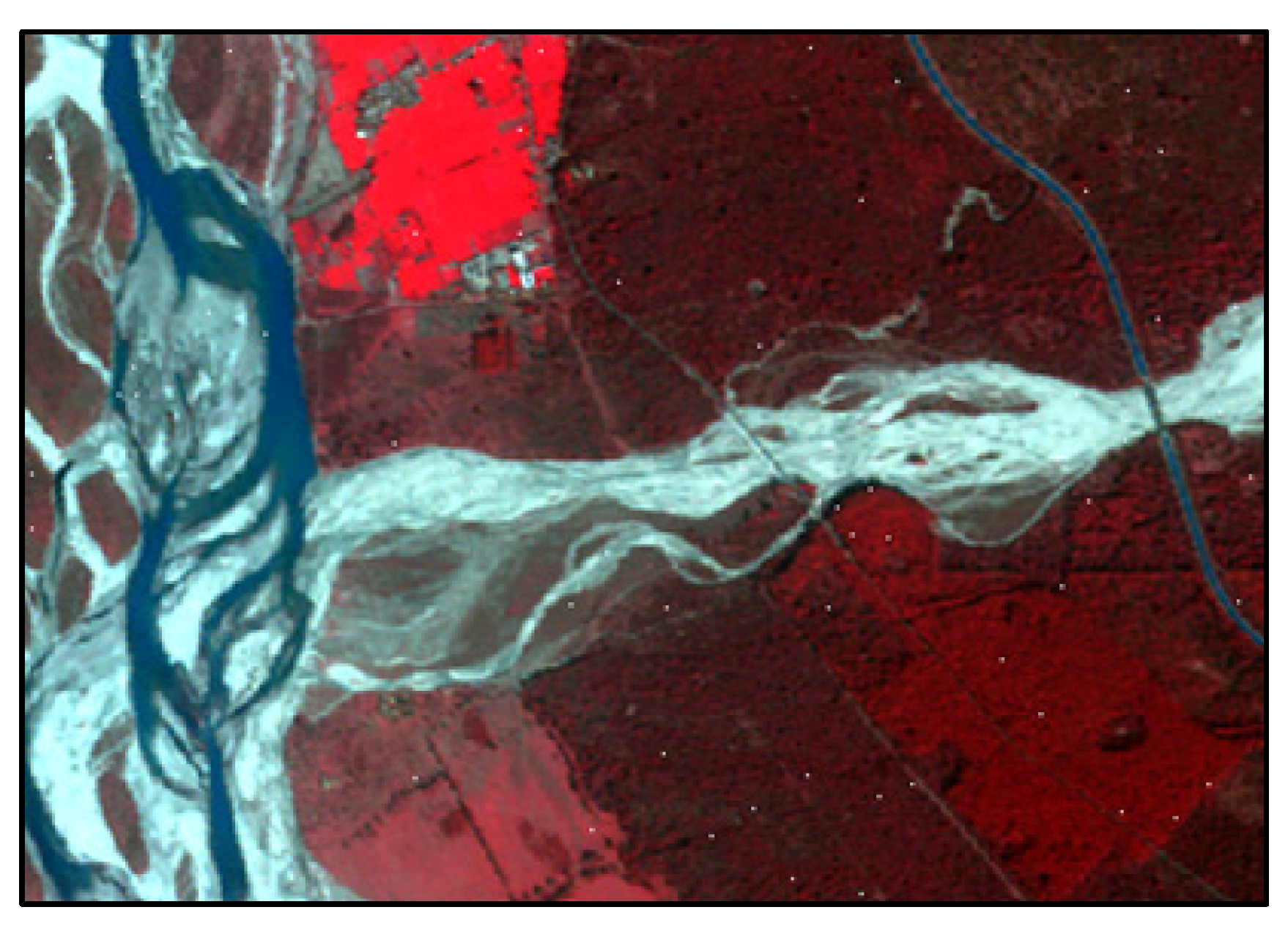
A multispectral satellite image acquired by Landsat-8 on 12 February 2015, with a spatial resolution of 30 m, was used for image classification (Figure 1b). The image covers an area located in Haridwar district of Uttarakhand state, India, extending from latitudes 29°48′48″N to 29°53′14″N and longitudes 78°9′56″E to 78°14′43″E (Figure 1a). A finer resolution Formosat-2 image of the same area with a spatial resolution of 8 m, acquired on 21 February 2015, was used for generating reference membership fraction images (Figure 1c). The area is diverse in terms of LULC classes present. Six land cover classes, namely, Dense Forest, Eucalyptus, Grassland, Riverine Sand, Wheat, and Water, were selected for our study. A training and test dataset consisting of random pixels from the Landsat-8 image was generated with the help of available field data.
2.2. Classification Algorithms
Theoretical explanations of the conventional fuzzy clustering algorithms FCM, and PCM, along with the details of FCM-based local spatial information algorithms (FCM-S, FLICM, and ADFLICM), and the proposed adaptations of these algorithms with PCM viz PCM-S, PLICM, and ADPLICM, respectively, are provided in the subsequent sub-sections. The algorithm descriptions are limited to an estimation of class membership values from supervised versions of these algorithms.
2.2.1. Fuzzy c-Means (FCM)
The FCM [9,10] is originally an unsupervised clustering algorithm, which finds fuzzy partitions and prototypes by minimizing the objective function. The optimal fuzzy clusters are obtained by minimizing the objective function in Equation (1).
The FCM objective function is subjected to the constraints in Equation (2).
where, is the matrix of cluster centres with its elements denoted by ; is the mean vector for cluster i; is a × fuzzy partition matrix representing the membership values of pixels per cluster; is the membership value of jth pixel for cluster i; is the total number of pixels; is the number of clusters; is the fuzzy weight, which controls the level of fuzziness and its value lies between 1 and infinity (the value tending to infinity produces absolutely fuzzy outputs while tending to unity produces hard or crisp outputs); is the Euclidean distance (dij2) between the jth pixel value and cluster mean .
The fuzzy membership, whose value ranges between 0 (low similarity grade) and 1 (high similarity grade), denotes the similarity a data point (pixel) shares with the cluster/class. The optimization of the FCM objective function yields Equation (3) for determining the membership function.
2.2.2. Possibilistic c-Means (PCM)
The PCM algorithm, developed by Krishnapuram and Keller [18], is a modification of the FCM clustering algorithm. PCM works on the possibilistic theory and thus relaxes the probabilistic constraint of FCM that forces the class memberships of a pixel to be dependent on one another. The objective function of the PCM algorithm is given in Equation (4) subjected to the conditions in Equation (5).
where is the “bandwidth” or “resolution” or “scale” parameter [57] that controls the shape and size of the cluster/class. Its value is selected depending on the distribution of pixels in each cluster. The definition of in Equation(6), with the value of being generally chosen to be 1, has been found to work well [57].
The membership function (Equation (7)) is derived by minimizing the objective function of PCM. Unlike in FCM, the membership value here signifies the pixel’s possibility of belonging to a cluster or its typicality to a cluster. In other words, the membership value in PCM is absolute while the membership value in FCM is relative.
The interpretation of in PCM is different from that in FCM. Increasing values in FCM signifies increased sharing of the pixels among all available clusters, while an increasing value in PCM signifies an increased possibility of all pixels belonging to a given cluster.
2.2.3. Fuzzy c-Means with Spatial Constraint (FCM-S)
The FCM-S proposed by Ahmed et al. [42] includes a spatial constraint term in the modified FCM objective function that forces the classification of the pixels to be influenced by the pixel values in the immediate neighborhood. The objective function of FCM-S is defined by Equation (8).
where is the set of neighbor pixels falling into the window around the pixel j; is the cardinality of ; is the parameter that controls the effect from the neighborhood; is the squared distance (dir2) between the pixel value and the cluster mean , where represents the rth neighbor in the neighboring window of .
2.2.4. Fuzzy Local Information c-Means (FLICM)
In the FLICM algorithm devised by Krinidis and Chatzis [44], a new fuzzy factor is introduced as a local (spatial and grey level) similarity measure for noise insensitivity and image detail preservation. The algorithm is free from empirically selected parameters. Its objective function is given in Equation (9).
where is the fuzzy factor (of the jth pixel for the ith class) that uses the spatial distance between the center pixel and the neighboring pixels in the local window to control the influence of the pixels in the neighborhood. is calculated using Equation (10).
is the spatial Euclidean distance between the centre pixel j and the neighboring pixel r; is the degree of membership of the rth neighbor pixel (of central pixel j) in cluster i.
2.2.5. Adaptive Fuzzy Local Information c-Means (ADFLICM)
The ADFLICM clustering algorithm [21] utilizes a fuzzy similarity measure derived from the spatial attraction model. Spatial attraction models are used to describe the spatial correlation between pixels in an image. The spatial attraction (SA) between two pixels j and r for class i is described by Equation (11).
The similarity measure of ADFLICM is defined by Equation (12), which is based on the spatial attraction model given in Equation (11).
The objective function of ADFLICM is described in Equation (13).
2.2.6. PCM-Based Local Spatial Information Classification Algorithms
The objective function of the standard PCM algorithm was modified to develop PCM-S, PLICM, and ADPLICM algorithms, similar to the modification of the FCM objective function in the FCM-S, FLICM, and ADFLICM algorithms, respectively. The objective functions were formulated and minimized in a fashion similar to the standard FCM/PCM classification algorithms. The necessary conditions were obtained for the objective functions of each algorithm to be at their local minimal extreme with respect to .
- (1)
- Possibilistic c-means with spatial constraint (PCM-S)
The objective function of the PCM algorithm was modified with the spatial constraint term from the FCM-S algorithm to develop the PCM-S algorithm. The PCM-S objective function is given in Equation (14).
To obtain the membership equation, the objective function had to be minimized with respect to . As the rows and columns of are independent of one another, minimizing the objective function with respect to is equivalent to minimizing the individual objective function in Equation (15) with respect to , provided that the resulting membership value lies in the interval [0,1] [18].
Differentiating Equation (15) with respect to and setting it to zero yielded the equation for the membership function given in Equation (16).
- (2)
- Possibilistic local information c-means (PLICM)
The PLICM algorithm was formulated by modifying the PCM algorithm with the fuzzy factor from the FLICM algorithm. The objective function of the PLICM algorithm is described in Equation (17).
The equation for fuzzy factor is similar to the FLICM algorithm, which is described by Equation (10). The membership function (Equation (18)) below is obtained for at its local minima with respect to .
- (3)
- Adaptive possibilistic local information c-means (ADPLICM)
An ADPLICM algorithm was formulated using the similarity measure with spatial attraction model as defined in the case of the ADFLICM algorithm. Spatial attraction () and similarity measure () equations for ADPLICM are the same as those of the ADFLICM algorithm, which correspond to Equations (11) and (12). The objective function for the ADPLICM algorithm is described in Equation (19).
The membership function of the ADPLICM algorithm obtained is given in Equation (20).
2.3. Methodology
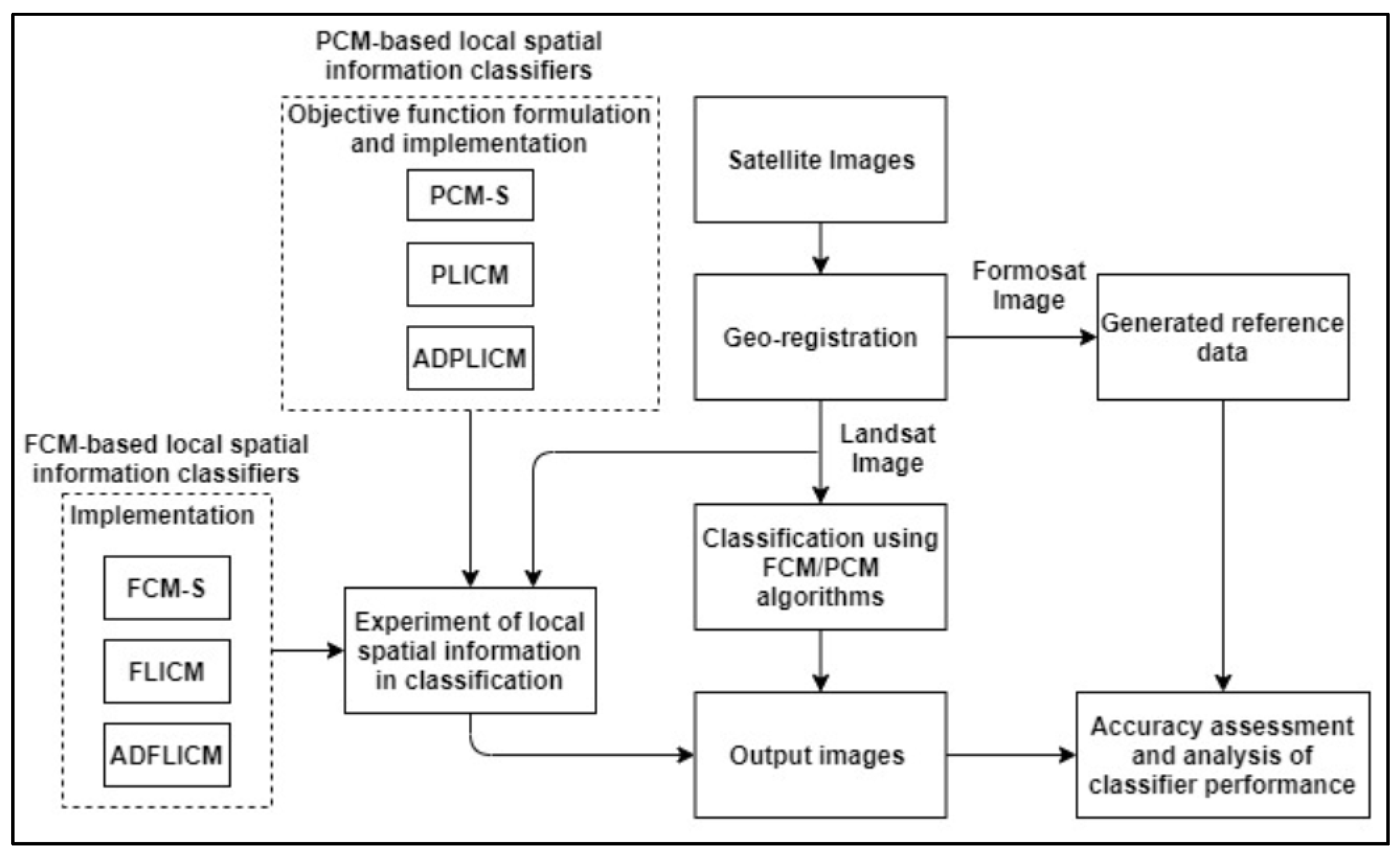
The adopted methodology used in this study is shown in Figure 2. The methodology steps involved pre-processing of satellite images, implementation of classification algorithms, optimization of algorithm parameters, and evaluation of algorithm performances by experimental analysis. All classification algorithms and accuracy assessment methods were implemented using Python 3.7 (libraries used: Rasterio, Numpy, Matplotlib, Math).
The Landsat-8 image used for classification and the Formosat-2 image used for the creation of reference membership fraction images were initially pre-processed. This included geo-referencing of Formosat-2 image and resampling to a 10 m spatial resolution using the Nearest Neighbor method so that the pixel sizes in the Formosat-2 image and the Landsat-8 image were in the ratio of 1:3. Image-to-image registration was subsequently performed using the Formosat-2 image chosen as the master image. The images were then cropped to the study area for further analysis.
The algorithm parameters, fuzzy factor , window size, and (in the case of FCM-S and PCM-S), were initially optimized for the classifiers to exploit their maximum potential. Owing to the disparity in the choice of the optimal value of in the literature [9,28,29], we followed an experimental strategy to estimate the best possible value of , in the interval [1.1,3], for which the highest classification accuracy was obtained. The window size and parameter , in FCM-S and PCM-S, were also optimized following a trial-and-error approach. The estimation of the optimal value of in the FCM-S algorithm without prior knowledge of noise was found to be difficult [44]. Larger values of were seen to generate more noise resistant outputs, while smaller values of were seen to generate outputs where image details were better preserved. Because of this, we followed an empirical approach to find the optimal value of as in other studies, where the FCM-S algorithm was studied [21,42,43,44]. The value of parameter was chosen by repeated testing in the interval of [0.2,8] and fixing the value from which maximum output accuracies from FERM and RMSE were obtained.
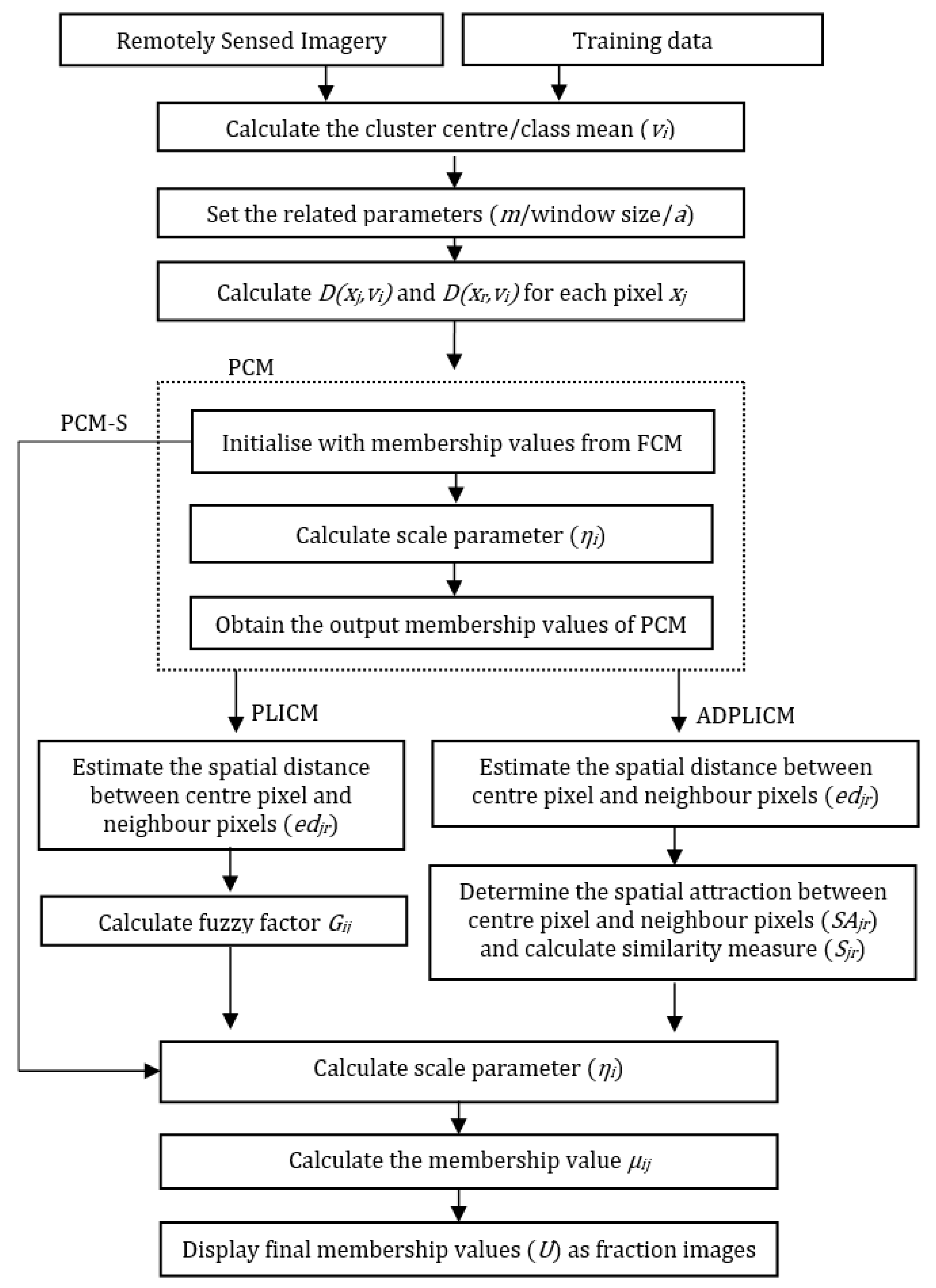
The flowcharts for the execution of the PCM-S, PLICM, and ADPLICM algorithms are presented in Figure 3. To initialize the PLICM and ADPLICM algorithms, the PCM algorithm was used. The supervised versions of the FCM, PCM, FCM-S, FLICM, and ADFLICM algorithms were also implemented for comparative analysis. The modification of unsupervised to supervised classification involved obtaining class centroids from input training data and estimating class memberships in a single step [17].
The performances of the local spatial information algorithms were examined for supervised classification in the soft (fuzzy) mode. The input image was separately classified using the FCM, PCM, FCM-S, FLICM, ADFLICM, PCM-S, PLICM, and ADPLICM classifiers for the identified six land cover classes. The accuracy matrices of the classifiers were estimated and compared to analyze the performance of the PCM-based local spatial information classifiers with the FCM-based local spatial information classifiers. The soft classification outputs from FCM and PCM were also included in the accuracy assessment to better assess the effect of including local spatial data into these standard classifiers. Furthermore, experiments were performed to evaluate all eight classifiers’ outputs in the presence of untrained classes and in the presence of isolated noisy pixels (pixels that are different from their neighboring pixels). The details of these experiments, along with the results, are explained in the next section.
As soft classification outputs represent the proportion of two or more classes in a pixel, conventional accuracy assessment methods, such as the confusion matrix [58] or kappa coefficient, could not be applied. Therefore, the overall accuracy of the fuzzy error matrix (FERM) [59] and RMSE (root mean square error) were used for assessing the accuracy of soft classified outputs generated by each algorithm with reference to the soft reference data. FERM has a layout similar to the conventional error matrix with the exception that it can have non-negative real numbers, which indicate the class proportions in the reference image and classified image, instead of non-negative integer values. The test dataset was carefully prepared to include pure pixels from homogenous regions of each class, isolated pixels, and pixels at the boundaries or edges of the classes.
3. Results
The performances of the PCM-S, PLICM, and ADPLICM classifiers were examined and compared with FCM-S, FLICM, ADFLICM, and the standard FCM/PCM classifiers through four experiments. The scenarios executed were the (1) supervised classification with all the identified classes, (2) supervised classification with untrained classes, (3) supervised classification for single class extraction, and (4) supervised classification in the presence of noise. It was observed that the optimal value of the fuzzy factor , for each classifier varied when the number of classes selected for classification varied. Hence different values were used for the same classifier in each of the scenarios executed.
3.1. Experiment 1: Supervised Classification with All the Identified Classes
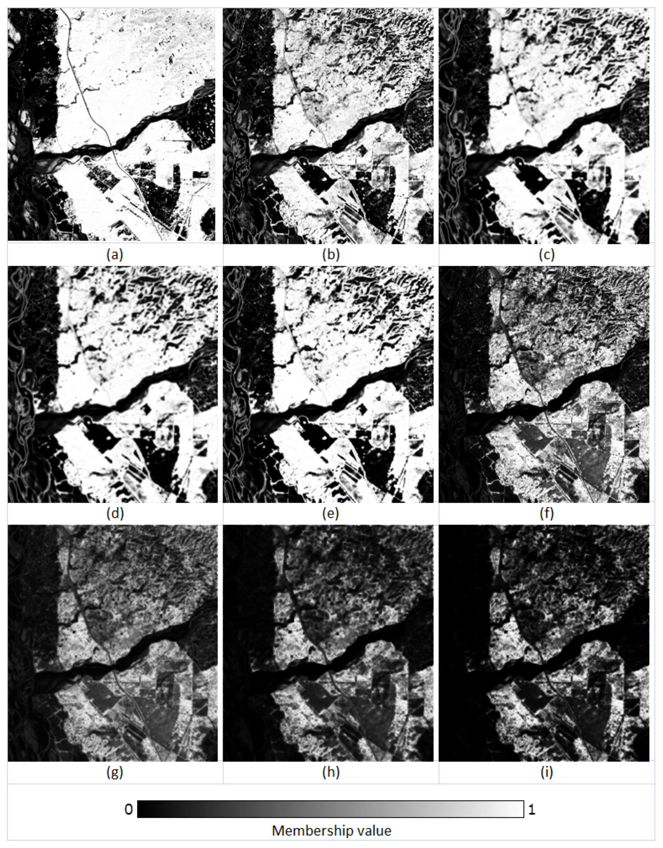
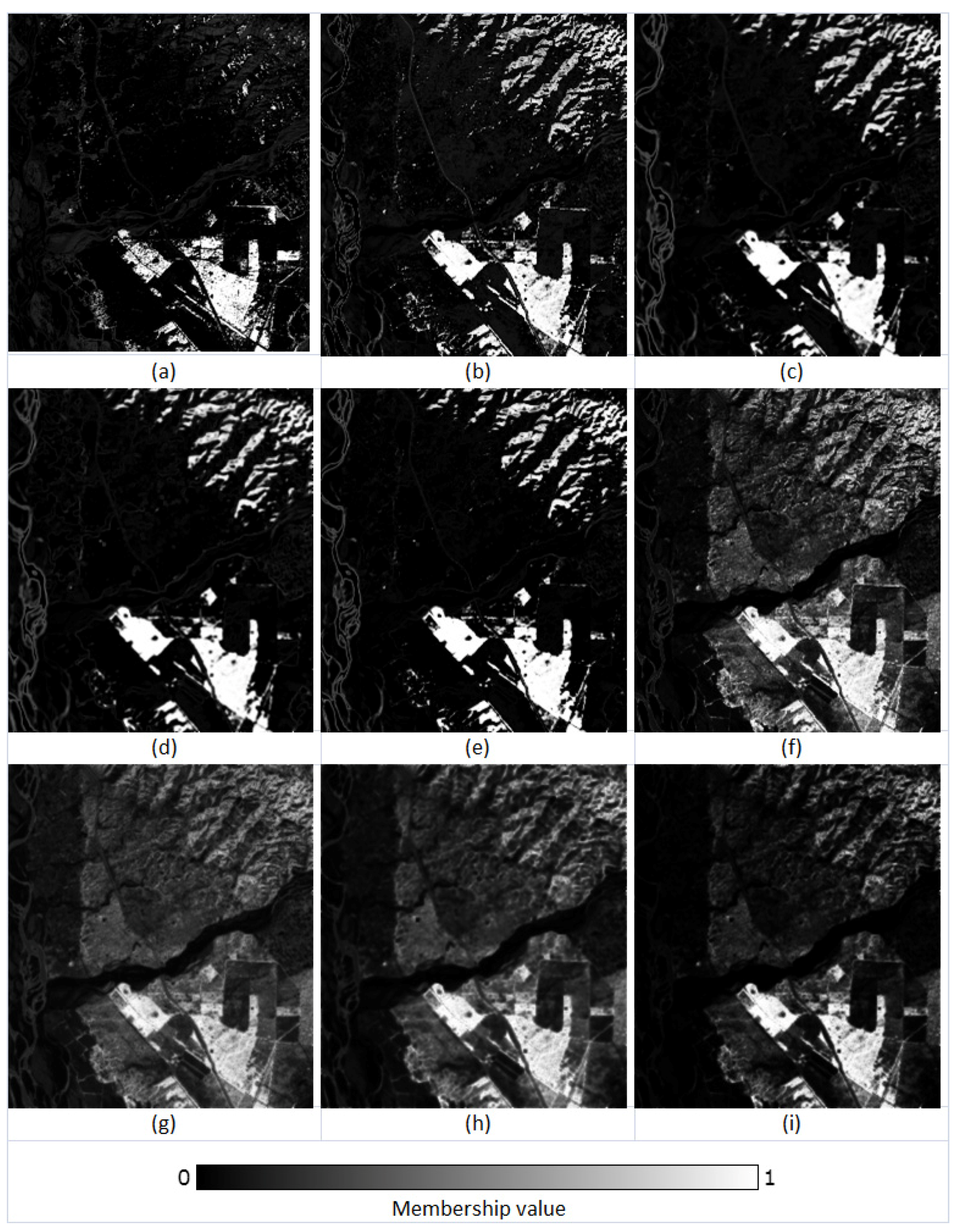
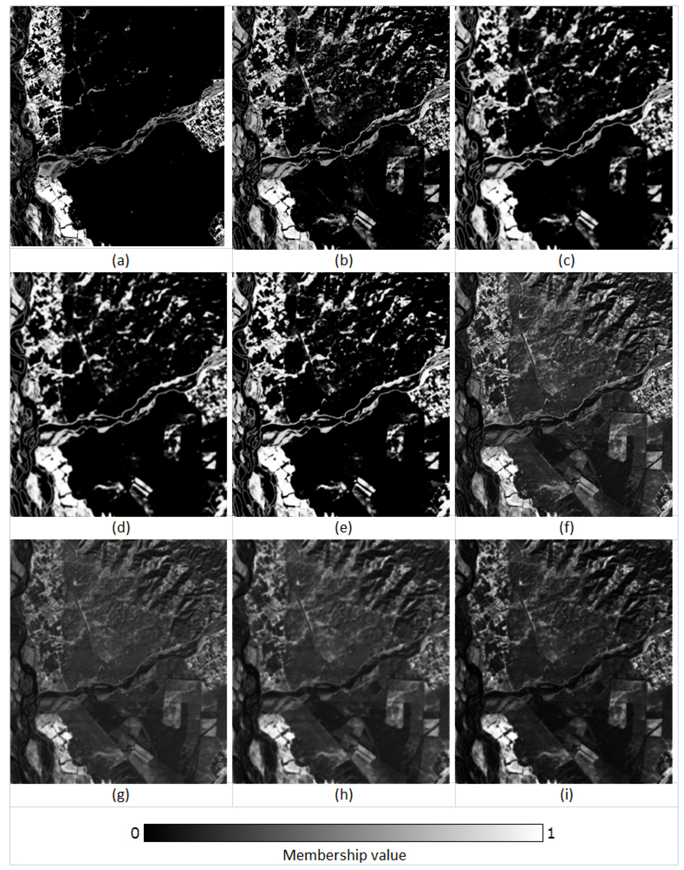
The sub-pixel land cover fraction outputs derived for all the six classes (Dense Forest, Eucalyptus, Grassland, Riverine Sand, Wheat, and Water) generated by the eight fuzzy classification algorithms are given in Figure 4, Figure 5, Figure 6, Figure 7, Figure 8 and Figure 9, respectively. The parameter values of all the algorithms were initially optimized by repeat testing and after careful examination of their effect on all the land cover classes (Table 1).
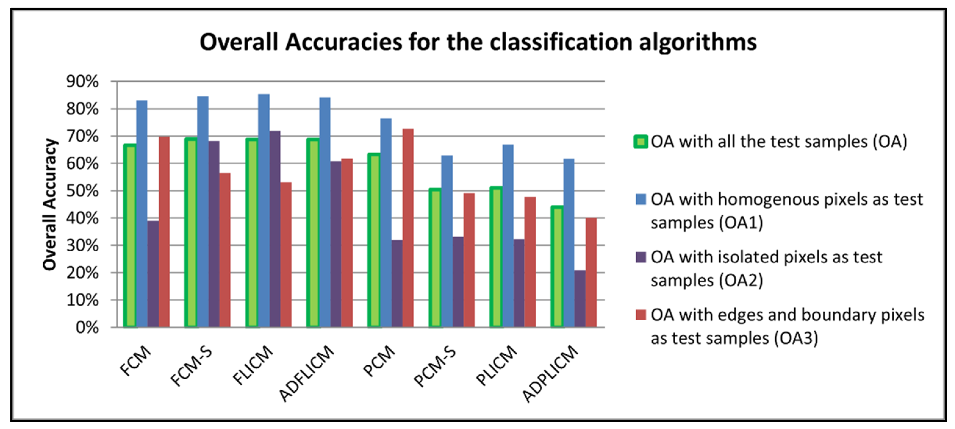
The FERM overall accuracy was used to quantitatively analyze the performance of the algorithms. The overall accuracy was calculated for each algorithm (1) while taking all the random test samples for accuracy assessment, (2) while taking only the homogenous pixels for testing, (3) while taking isolated pixels as test samples, and (4) while taking the edges and boundary pixels as test samples. The overall accuracies for the four different cases discussed above are denoted by OA, OA1, OA2, and OA3 correspondingly (Table 2 and Figure 10). The overall accuracies, in general, for all the algorithms were seen to be higher (OA1) when test data consisted of pure pixels from homogenous regions and lower (OA3) when test data consisted of mixed pixels, whose exact ground proportion was not known. While including more pure test pixels from homogenous regions could improve the general overall accuracy, the purpose of the study was to compare the algorithm performance for different cases. The overall poor accuracies of algorithms do not have a considerable impact on the conclusion and inferences of this comparative study.
The FCM classifier variants were seen to produce higher accuracies in this scenario. The FCM-S, FLICM, and ADFLICM showed greater overall accuracies while all the random test sample pixels were used for accuracy assessment. Although FLICM and FCM-S were effective in removing isolated pixels and their classification performances were slightly higher than that of conventional FCM in homogenous regions (Figure 10 and Figure 11), they produced smoother outputs, which resulted in the loss of image details, such as edges and boundaries (Figure 12). As inferred by H. Zhang et al. [21] in their study, the ADFLICM algorithm showed acceptable performance compared to FCM-S and FLICM in terms of handling isolated pixels while simultaneously retaining the image details (Figure 12). While the overall accuracies of PCM and PCM-based local spatial information classifiers were lower, the PCM classifier was seen to retain the edges and boundary pixels better than the FCM variants (OA3 in Figure 10).
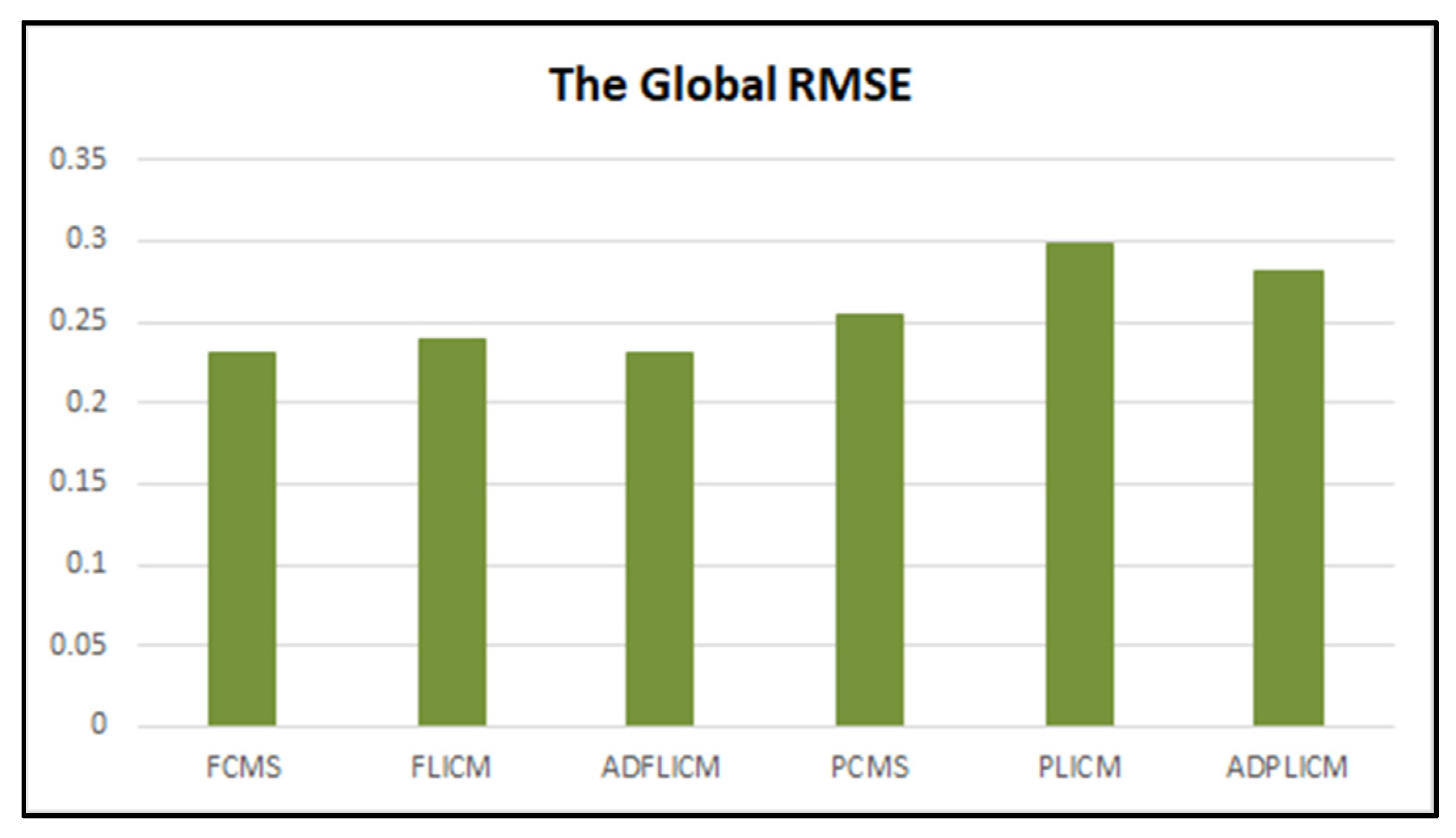
The comparison of global RMSE values estimated for fuzzy local spatial information classifiers also implied the superiority of the FCM-based local spatial classifiers over the PCM-based local spatial information classifiers (Table 3 and Figure 13). The PCM-S, PLICM, and ADPLICM generated higher RMSE values, while the FCM-S, FLICM, and ADFLICM generated lower RMSE values.
3.2. Experiment 2: Supervised Classification with Untrained Classes
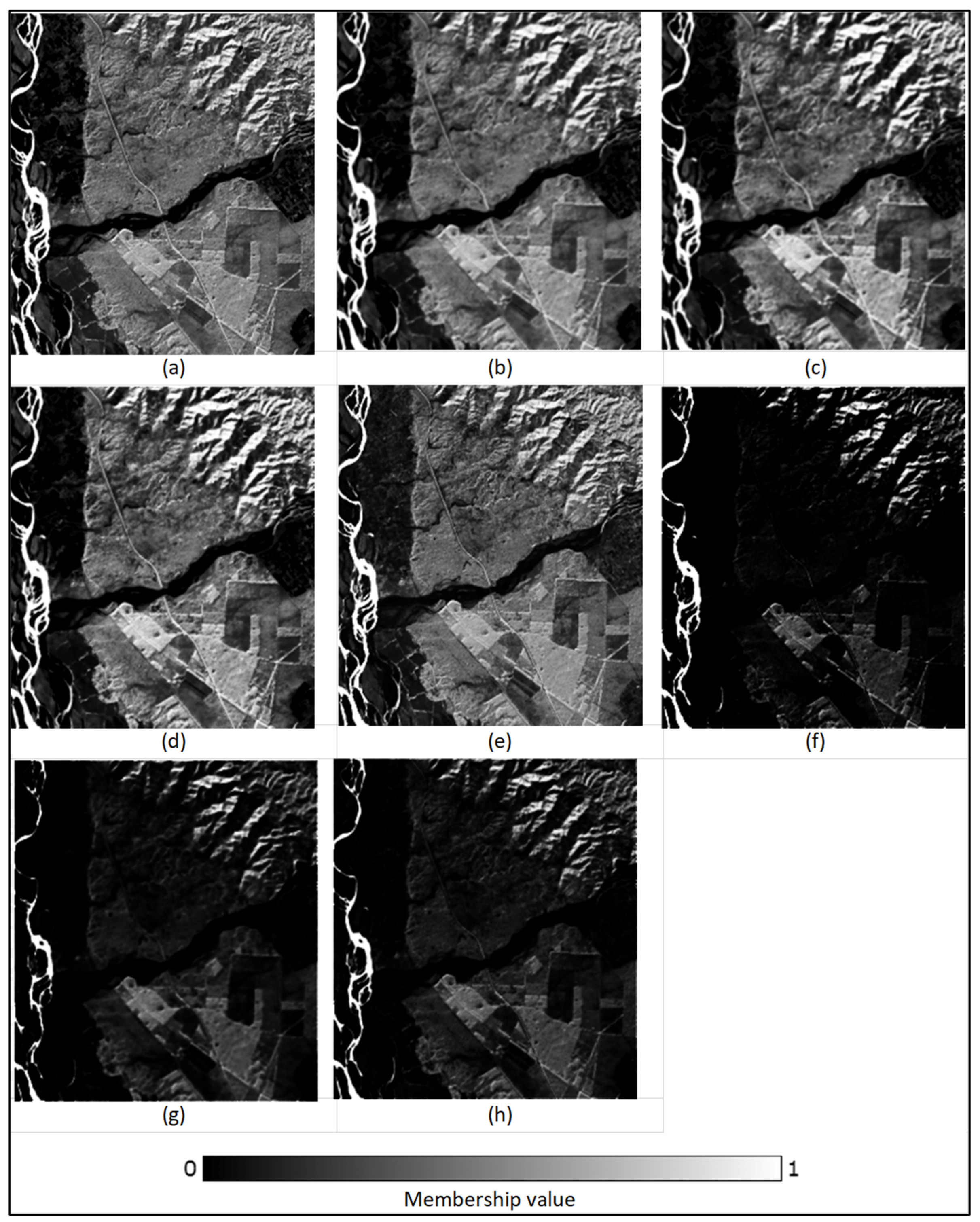
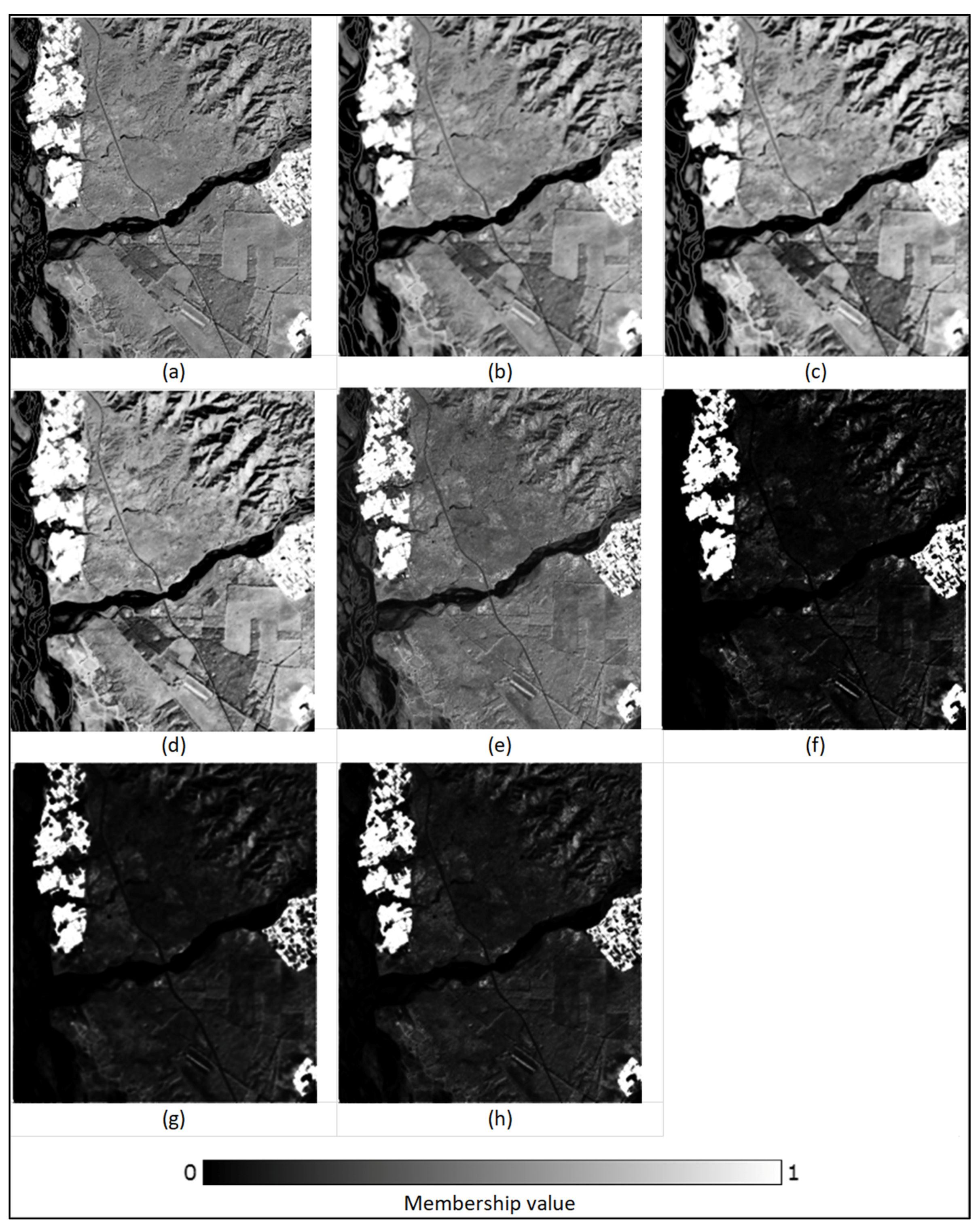
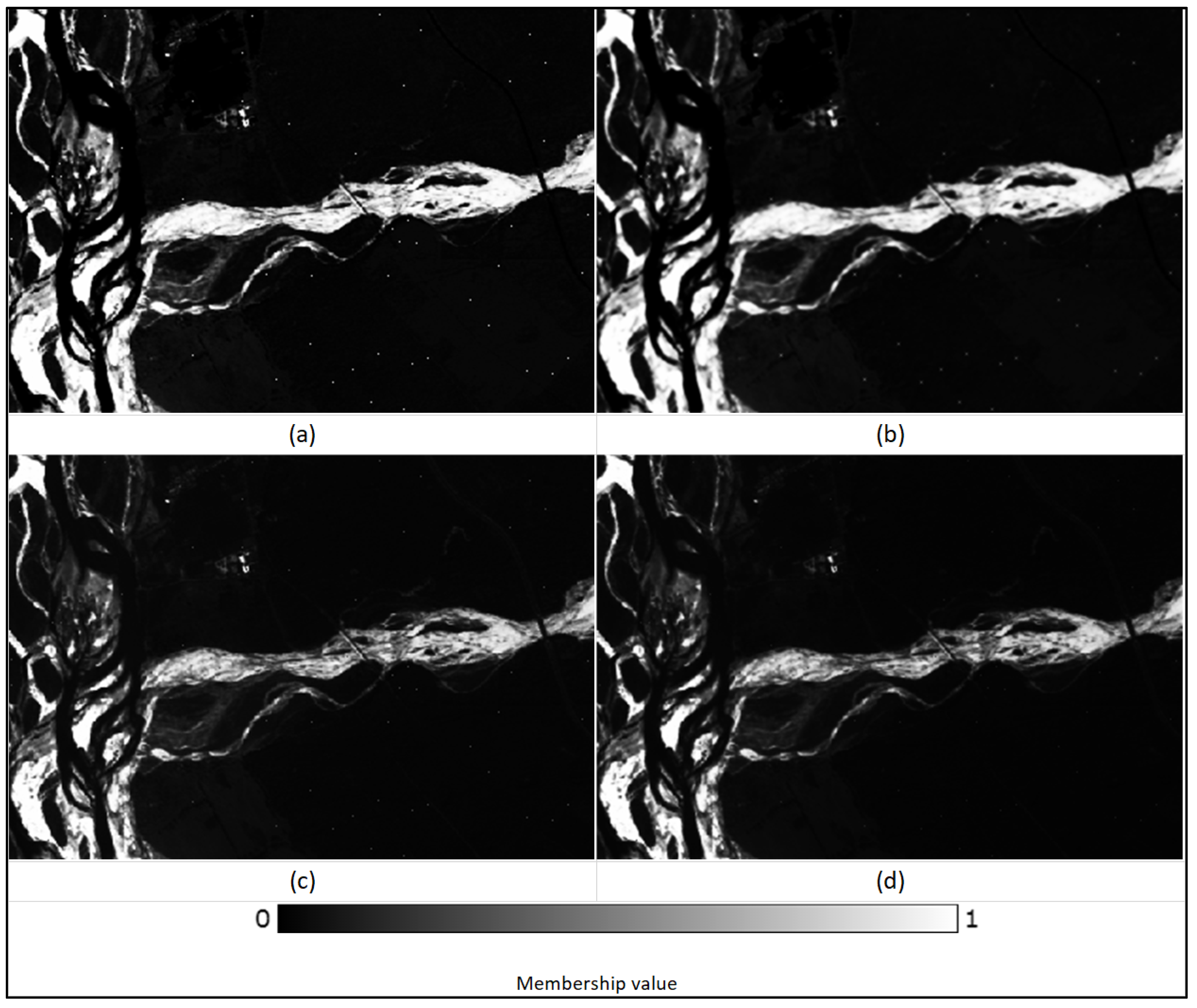
To understand the performance of the fuzzy local spatial information algorithms in the presence of untrained classes, training pixels from a few information classes were excluded from the training data. Three classes ‘Riverine Sand’, ‘Water’, and ‘Wheat’ were defined, and the training pixels for the remaining classes were removed from the training data before classification. This meant that the pixels in the study area from the omitted classes from training data ideally should be considered as noisy pixels by the classifiers. The output fraction images for the three classes mentioned above were generated by each of the eight classifiers FCM, FCM-S, PCM, PCM-S, PLICM, and ADPLICM separately (Figure 14, Figure 15 and Figure 16). The values chosen for were 1.5, 1.2, 1.5, and 1.4, respectively, for PCM, PCM-S, PLICM, and ADPLICM algorithms. The remaining parameter values were the same as those given in Table 1.
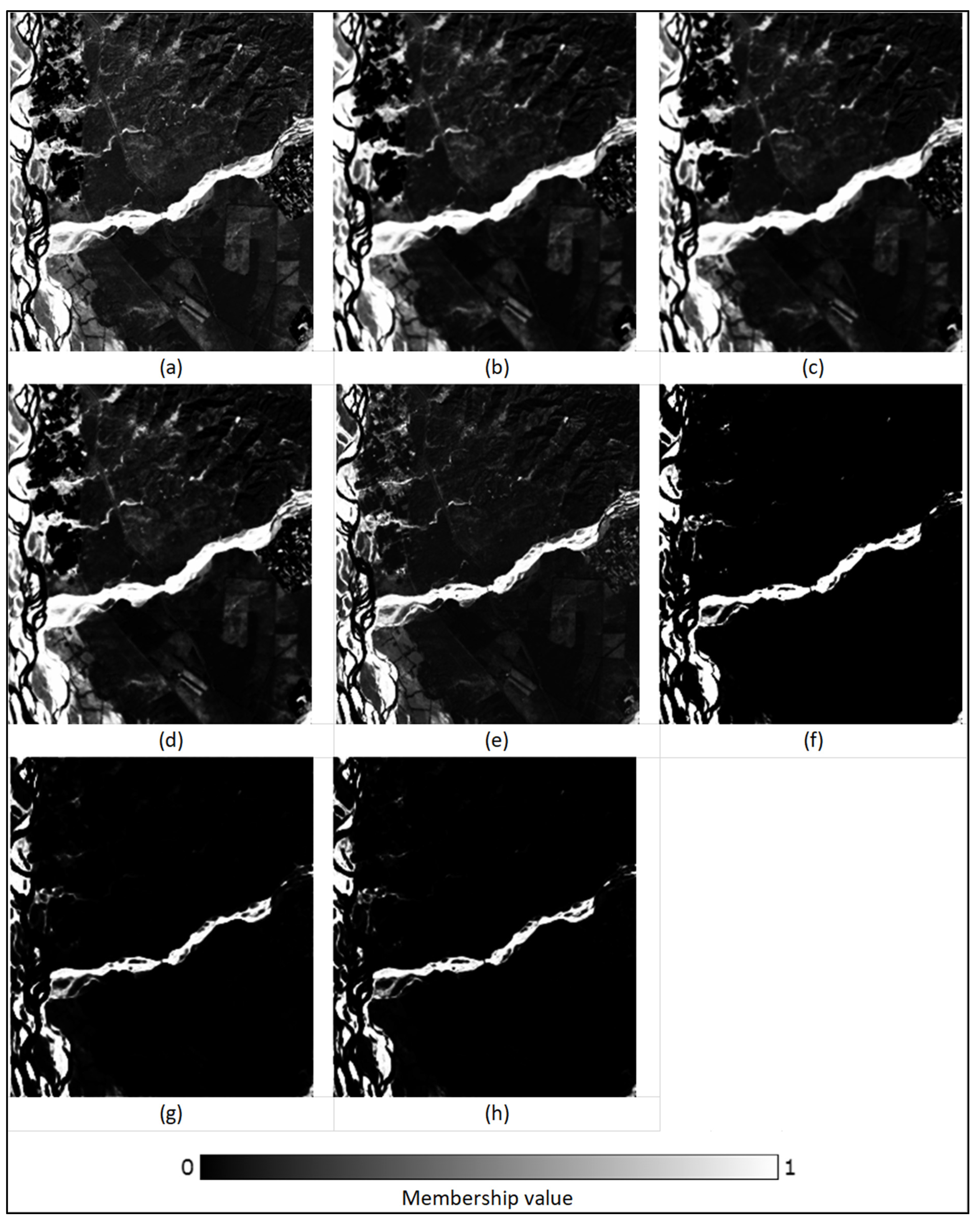
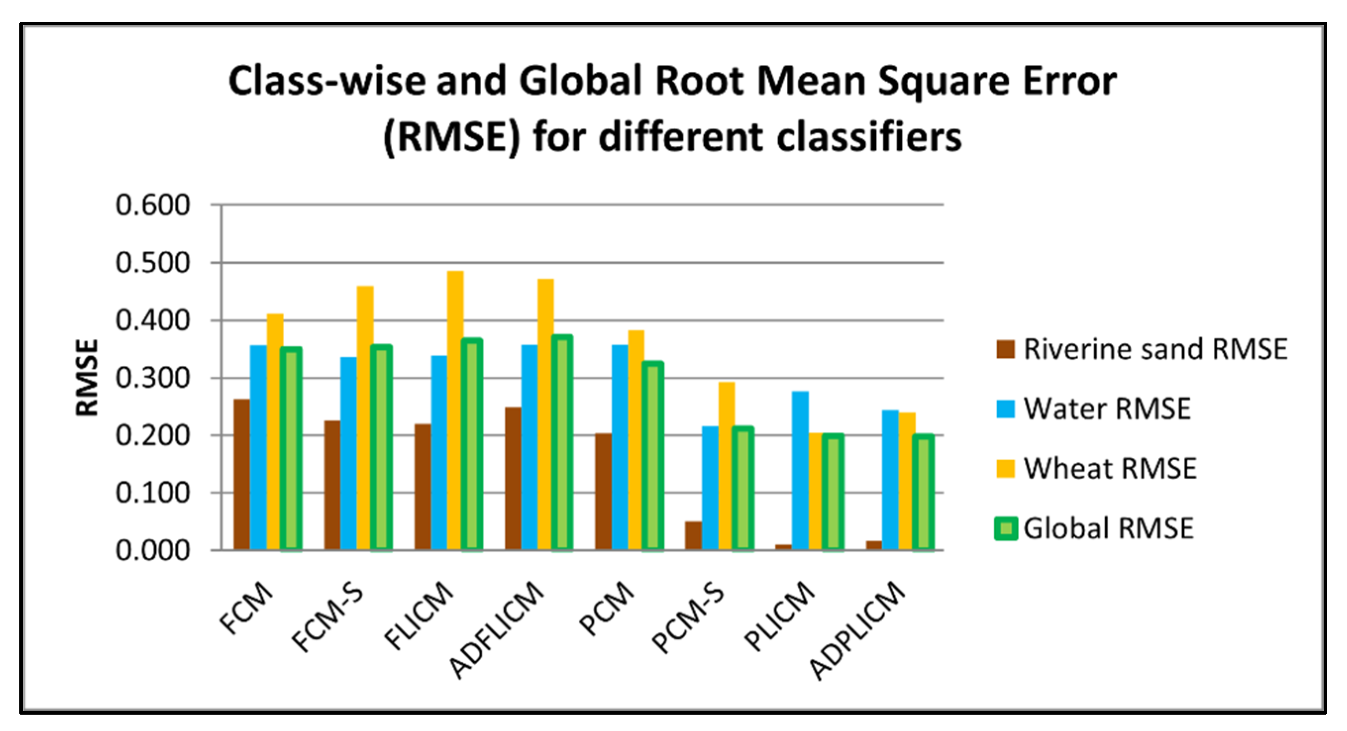
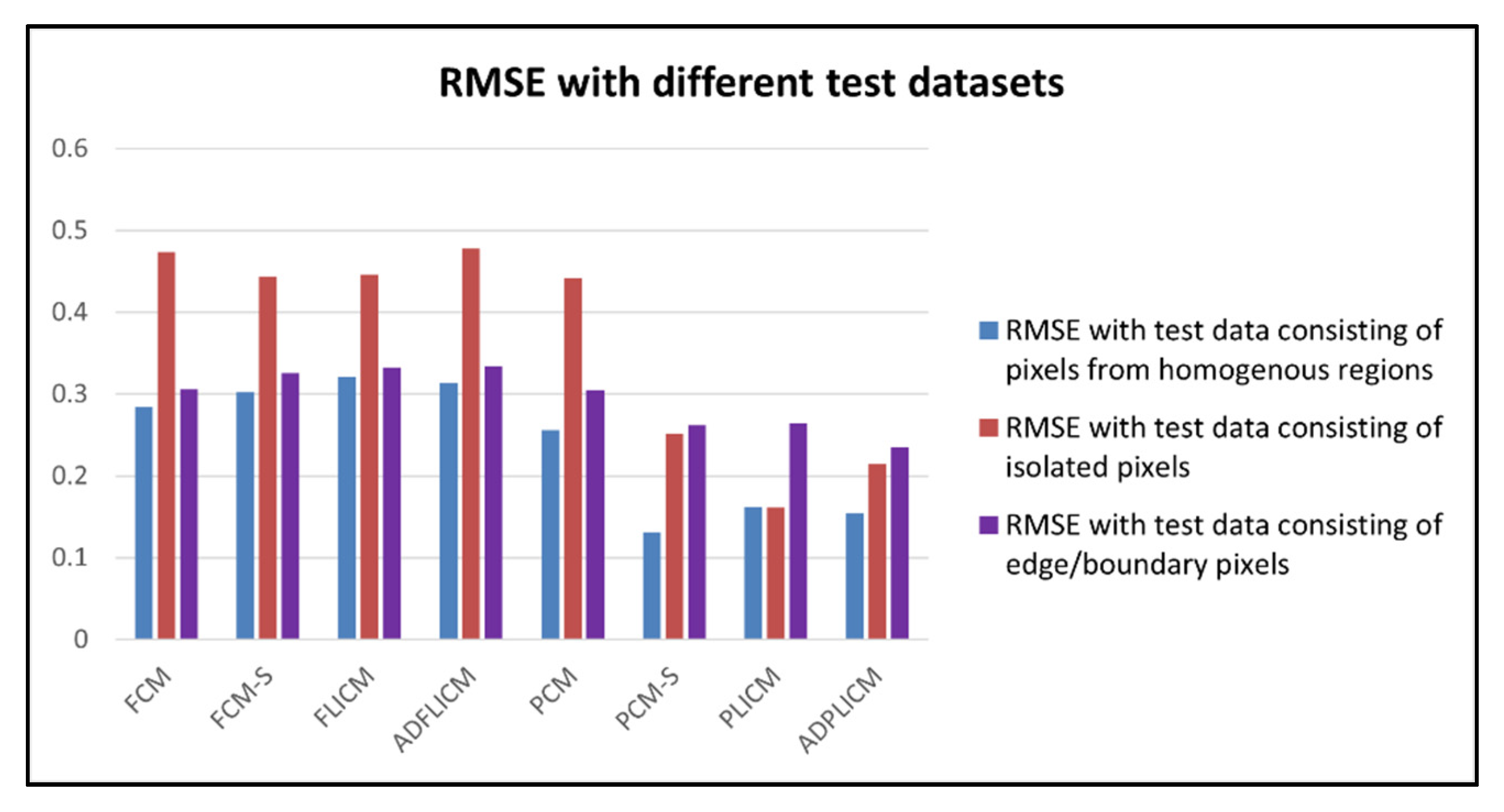
The global and class-wise RMSE values were estimated for outputs from each classifier (Table 4 and Figure 17). The PCM-based local spatial information classifiers, PCM-S, PLICM, and ADPLICM, exhibited lower RMSE values, which meant that there was less disparity between the output fraction images generated from these classifiers and the corresponding reference fraction images. Although the PLICM classifier was seen to be slightly advantageous over the other two algorithms in terms of global RMSE value, the class-wise RMSE for the Water class and visual interpretation suggested a significant loss in membership values for Water pixels with the PLICM classifier. To better analyze the performance of PCM-based local spatial information classifiers, RMSE calculation was repeated with test pixels from homogenous regions, noisy test pixels, and test pixels from borders and edges of the LULC classes (Figure 18). The RMSE values obtained in this case affirmed that the loss of image details was maximal in the PLICM classifier among the PCM-based local spatial information classifiers and minimal in the ADPLICM classifier. The RMSE values with noisy test pixels were, in general, lower for the PCM-based local spatial information classifiers, with PLICM producing the lowest value. The ADPLICM classifier was seen to perform better in retaining the image details among the PCM-based local information classifiers.
3.3. Experiment 3: Supervised Classification for Single Class Extraction
Extracting a single land cover class might often be required in remote sensing applications. The FCM algorithm and its variants cannot be used to extract a single class from satellite images because of the probabilistic membership constraint in Equation (2), which forces the membership values of the pixels in the single output fraction image generated to be one. In contrast, the PCM algorithm proved viable for one-class classification [60]. For the extraction of a single LULC class from the input dataset, PCM, PCM-S, PLICM, and ADPLICM were used in this study. The training data for the ‘Wheat’ class alone was given as an input to the classifiers, and output fraction images for the standard PCM and the three PCM-based local spatial information classification algorithms were generated (Figure 19). The RMSE values obtained for outputs of the classifiers are given in the table below (Table 5). Based on the RMSE value, PLICM/ADPLICM was observed to be the better performing classifier in extracting the ‘Wheat’ class.
3.4. Experiment 4: Supervised Classification in the Presence of Noise
The local spatial information algorithms were investigated with a noisy image to evaluate their noise tolerance ability. The Formosat-2 image was corrupted with noisy pixels or isolated pixels whose DN values differed substantially from the surrounding pixels. This was accomplished by setting the DN values of random pixels in the image to “255” in all bands, thereby resulting in random noise pixels appearing as ‘white dots’ in the image (Figure 20). The noisy image was then separately classified using FCM, FCM-S, PCM, and PCM-S classifiers with the training data of three classes (‘Riverine Sand’, ‘Water’, and ‘Wheat’). FCM-S and PCM-S were chosen among the local spatial information classifiers since the effect from the neighboring pixels for classification could be controlled using the parameter , unlike the other local spatial information classifiers. The value for the parameter was set to 2 in FCM-S and 0.2 in PCM-S. The value of 1.6 was used in all four classifiers.
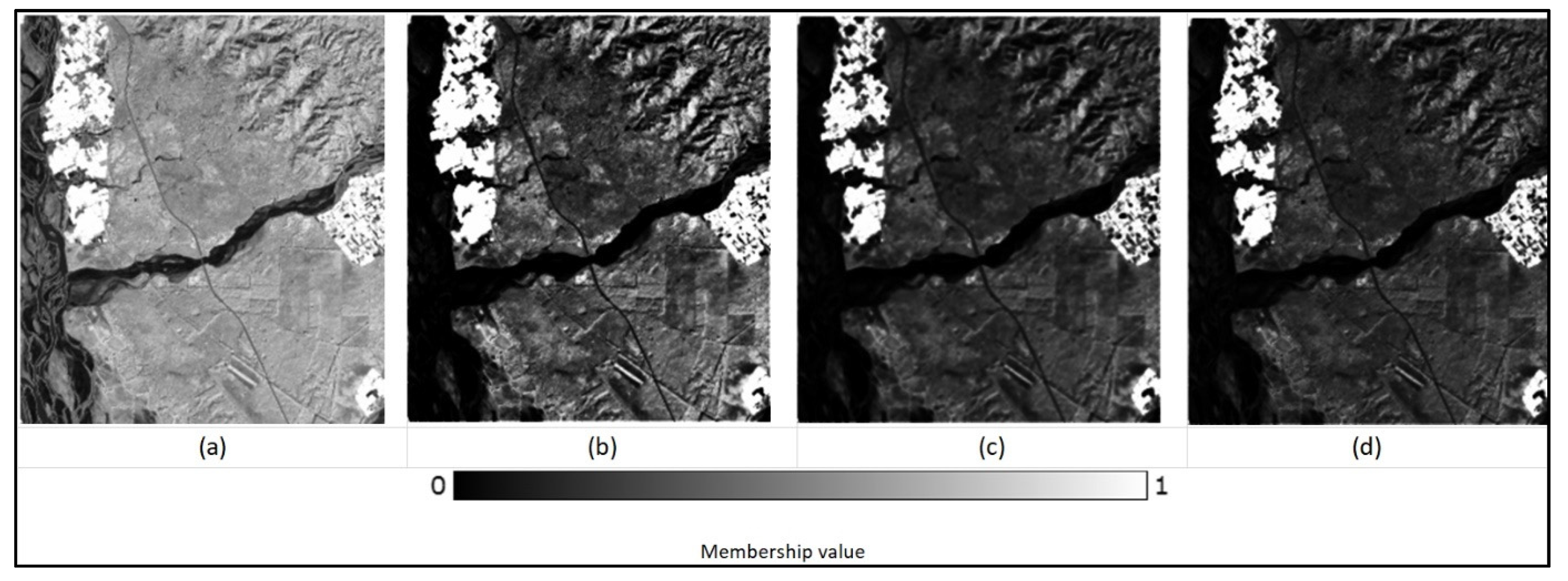
The noisy pixels in the input image appeared as isolated pixels in the classification outputs, predominantly in the class proportion images generated for ‘Riverine Sand’. The membership fraction images of the class ‘Riverine Sand’ generated by FCM, FCM-S, PCM, and PCM-S classifiers are shown below (Figure 21). The isolated pixels were most evident in the FCM output, owing to their high membership values in the class ‘Riverine Sand’ relative to other defined classes. The noise was seen to be less noticeable in the FCM-S classifier output as compared to the FCM output, very minimal in the PCM output, and negligible in the PCM-S output.
4. Discussion
While the choice of reference data and accuracy assessment methods hugely influence the analysis and conclusions drawn from a study, a few specific observations of the results and the accuracy matrices obtained during the scenarios executed in our study are described below. The overall accuracy of FERM and the visual interpretation demonstrated that the three FCM-based local spatial information classifiers (FCM-S, FLICM, and ADFLICM) produced more accurate results, followed by the FCM classifier for classifications with all the six LULC classes. On the contrary, the output quality of the FCM spatial variants degraded significantly in the presence of untrained classes. However, the land cover compositions obtained from the PCM-based local spatial information classifiers were in close agreement with the reality/reference image when a few classes were excluded from training. The three PCM-based local spatial information classifiers (PCM-S, PLICM, and ADPLICM) produced similar RMSE values, which were lower than those of the standard PCM classifier. In other words, the effectiveness of the PCM algorithm in the presence of untrained classes and in handling isolated pixels (noise) was seen to have further improved by incorporating it with local spatial information. While PLICM and ADPLICM were seen to be slightly advantageous in creating accurate land cover class compositions, the empirically set parameter in PCM-S allowed control of the neighborhood effect, depending on the noise intensity in the input image. Among the PCM-based local spatial information classifiers, ADPLICM was seen to preserve maximum image details, such as the ADFLICM of the FCM-based local spatial information classifier.
It was not possible to make a general comparison of the performance of the FCM-based local spatial information classifiers with those of PCM-based local spatial information classifiers since the fundamental behaviors of their corresponding base classifiers were different. The fraction outputs in the FCM classifier illustrated how well every image pixel was accommodated among the existing classes, while the fraction images of the classes in the PCM classifier focused on allocating every image pixel to that class. Due to this, the FCM variants performed well when all the classes were defined, but the performance degraded when a few classes were excluded from training. As Foody [44] concluded in his study, the PCM classifier sometimes is more appropriate than the FCM classifier, although the PCM produces less accurate land cover estimates when all classes are defined. Similar results were observed in our study, in which the PCM and the PCM-based local spatial information classifiers produced lower accuracies than the FCM classifier variants when all classes were defined (Experiment 1). However, the performance of the PCM classifier variants was seen to improve in the presence of untrained classes, as the membership values in these classifiers are calculated using the absolute measure instead of the relative measures [17]. The typical membership of the PCM makes it naturally immune to noise, and hence it results in a more accurate representation of reality in ambiguous environments, regardless of the number of training classes available [16,18]. Further, the typicality of PCM membership values was seen to be enhanced when integrated with local spatial information. In other words, the PCM-based local spatial information classifiers were observed to be even more advantageous in cases where generally the conventional PCM classifier performed better than the FCM variants. To summarize, the FCM-based local spatial information classifiers and PCM-based local spatial information classifiers worked well in situations where their respective base classifier performed better, disregarding the obvious smoothing that resulted from integration with spatial contextual information.
The fuzzy local spatial information classifiers investigated in this study were observed to have obvious advantages over the conventional fuzzy classifiers in handling the noisy pixels and isolated pixels that occurred due to spectral confusions. Nevertheless, there was a loss of image details in these local spatial information classifier outputs due to smoothing in the classes with lesser spatial extent, such as the ‘Water’ class, and also at the edges and boundaries of classes. The new PCM-based local spatial information classifiers showed extreme loss of image details and poor performance among all the classifiers during supervised classifications with training pixels from all the available landcover classes. However, these classifiers were found to be more efficient than the other fuzzy classifiers at handling noise and producing accurate fuzzy classification outputs during supervised classifications in the presence of untrained classes. Overall, the new PCM-based local spatial information classifiers might be the right choice over existing PCM, FCM, or the FCM-based local spatial variants in the presence of untrained classes and for single class extraction.
While this study elucidates the performance of PCM-based local spatial information algorithms and a few of their advantages, some major limitations of the study need to be acknowledged. First, the PCM performance greatly depends on its initialization. FCM, which is said to provide sensible initialization and scale estimate in less contaminated data [57], was used for initializing the PCM algorithm and hence the outputs of PCM and its variants were seen to produce different class proportion images on inclusion/exclusion of training classes for classification. Second, limited approaches have been explored for incorporating local spatial information in the PCM algorithm with measures that use the spatial Euclidean distance between the center pixel and neighboring pixels. This study could be extended to exploit measures such as the correlation among the pixels to control the effect of neighboring pixels on the center pixel. Third, a small study area in India was chosen for investigating the new algorithms, as the area is well-known and hence suitable for making a relative analysis of results from the existing and new algorithms. The evaluation could be extended to other areas with a wider set of LULC classes. Fourth, there is no standard process for accuracy assessment for soft classification. Methods for the creation of the soft reference data and accuracy assessment of the soft classified outputs are still open research areas. We mainly used RMSE for obtaining a comparative judgment and have not performed any statistical analysis tests on the data or results obtained. Performing appropriate statistical significance tests correctly and drawing inferences cautiously using such tests could provide validity of the results [61].
5. Conclusions
Relevant information processing depends on good representation methods for information and efficient processing algorithms. Over decades, classifiers have been developed to improve the extraction of useful information from remote sensing imagery. In addition to spectral information, ancillary data, such as spatial-contextual information, has been seen to greatly enhance the classifier’s performance. The primary aim of this study was to investigate the effect of incorporating local spatial information into the PCM algorithm using simpler methods and to evaluate the benefits of the new PCM-based local spatial information classifiers over the existing FCM-based local spatial information classifiers. The algorithms PCM-S, PLICM, and ADPLICM, were developed for the classification and compared with the existing FCM-S, FLICM, and ADFLICM classifier outputs. To substantiate the advantages of integrating local spatial information for classification, the conventional FCM and PCM classifiers were also included in the assessment. Trials were performed to evaluate and compare the output of all the eight classifiers with all the classes, in the presence of untrained classes, and upon the introduction of isolated pixels. While it was not possible to comment on which classifier consistently gave better classification results, PCM-based local spatial information classifiers were observed to produce higher accuracies in the presence of untrained classes and in the presence of noise. The PLICM and ADPLICM classifiers producing lower global RMSE values, with ADPLICM being better at image detail preservation and PLICM being efficient at handling isolated pixels, generated more accurate class proportions for classifications in the presence of untrained classes and for extracting a single land cover class. At the same time, the adjustable parameter in the PCM-S classifier allowed the control of the classifier’s tolerance to input noise. In general, the performance of the PCM classifier was demonstrably improved as the overall RMSE value was seen to have reduced by more than 0.1 by integrating it with spatial information. Likewise, the RMSE values obtained for the three PCM-based local spatial information classifiers in the presence of untrained classes measured around 0.20, whereas for FCM-based local spatial information classifiers, the RMSE values obtained were in the range of 0.35–0.37. Therefore, there is a huge potential for the PCM classifier integrated with local spatial information to generate land cover compositions that are closer to reality and with much clearer management of outliers. In other words, PCM spatial information classifiers could produce better classification results than conventional PCM, FCM, or FCM variants, especially in the absence of an exhaustive set of information classes for training.
Author Contributions
Conceptualization, A.K., A.M. and P.J.; methodology, A.M. and A.K.; software, A.M.; validation, A.K., A.M. and P.J.; formal analysis, A.M.; writing—original draft preparation, A.M.; writing—review and editing, A.K. and P.J.; visualization, A.M.; supervision, A.K. and P.J. All authors have read and agreed to the published version of the manuscript.
Funding
This research received no external funding.
Institutional Review Board Statement
Not applicable.
Informed Consent Statement
Not applicable.
Data Availability Statement
Not applicable.
Acknowledgments
We thank the International Institute of Spatial Lifecourse Epidemiology (ISLE) for research support. We also thank Suzanne Buckley for improving the language of the manuscript.
Conflicts of Interest
The authors declare no conflict of interest.
References
- Campbell, J.B.; Wynne, R.H. Introduction to Remote Sensing, 5th ed.; Guilford Publications: New York, NY, USA, 2011; ISBN 978-1-60918-176-5. [Google Scholar]
- Zhang, J.; Foody, G.M. Fully-fuzzy supervised classification of sub-urban land cover from remotely sensed imagery: Statistical and artificial neural network approaches. Int. J. Remote Sens. 2001, 22, 615–628. [Google Scholar] [CrossRef]
- Wang, F. Fuzzy supervised classification of remote sensing images. IEEE Trans. Geosci. Remote Sens. 1990, 28, 194–201. [Google Scholar] [CrossRef] [Green Version]
- Foody, G.M.; Doan, H.T.X. Variability in Soft Classification Prediction and its implications for Sub-pixel Scale Change Detection and Super Resolution Mapping. Photogramm. Eng. Remote Sens. 2007, 73, 923–933. [Google Scholar] [CrossRef] [Green Version]
- Lu, D.; Weng, Q. A survey of image classification methods and techniques for improving classification performance. Int. J. Remote Sens. 2007, 28, 823–870. [Google Scholar] [CrossRef]
- Li, M.; Zang, S.; Zhang, B.; Li, S.; Wu, C. A Review of Remote Sensing Image Classification Techniques: The Role of Spatio-contextual information. Eur. J. Remote Sens. 2014, 47, 389–411. [Google Scholar] [CrossRef]
- Zadeh, L.A. Fuzzy sets. Inf. Control 1965, 8, 338–353. [Google Scholar] [CrossRef] [Green Version]
- Foody, G.M. Sub-Pixel Methods in Remote Sensing. In Remote Sensing Image Analysis: Including The Spatial Domain; De Jong, S.M., Van der Meer, F.D., Eds.; Springer: Dordrecht, The Netherlands, 2004; pp. 37–49. ISBN 978-1-4020-2560-0_3. [Google Scholar]
- Bezdek, J.C.; Ehrlich, R.; Full, W. FCM: The fuzzy c-means clustering algorithm. Comput. Geosci. 1984, 10, 191–203. [Google Scholar] [CrossRef]
- Bezdek, J.C. Pattern Recognition with Fuzzy Objective Function Algorithms; Springer: Boston, MA, USA, 1981; ISBN 978-1-4757-0452-5. [Google Scholar]
- Atkinson, P.M.; Cutler, M.E.J.; Lewis, H. Mapping sub-pixel proportional land cover with AVHRR imagery. Int. J. Remote Sens. 1997, 18, 917–935. [Google Scholar] [CrossRef]
- Bastin, L. Comparison of fuzzy c-means classification, linear mixture modelling and MLC probabilities as tools for unmixing coarse pixels. Int. J. Remote Sens. 1997, 18, 3629–3648. [Google Scholar] [CrossRef]
- Cannon, R.L.; Dave, J.V.; Bezdek, J.C.; Trivedi, M.M. Segmentation of a Thematic Mapper Image Using the Fuzzy c-Means Clusterng Algorthm. IEEE Trans. Geosci. Remote Sens. 1986, GE-24, 400–408. [Google Scholar] [CrossRef]
- Fisher, P.F.; Pathirana, S. The ordering of multitemporal fuzzy land-cover information derived from landsat MSS data. Geocarto Int. 1993, 8, 5–14. [Google Scholar] [CrossRef]
- Foody, G.M. Approaches for the production and evaluation of fuzzy land cover classifications from remotely-sensed data. Int. J. Remote Sens. 1996, 17, 1317–1340. [Google Scholar] [CrossRef]
- Ibrahim, M.A.; Arora, M.K.; Ghosh, S.K. Estimating and accommodating uncertainty through the soft classification of remote sensing data. Int. J. Remote Sens. 2005, 26, 2995–3007. [Google Scholar] [CrossRef]
- Foody, G.M. Estimation of sub-pixel land cover composition in the presence of untrained classes. Comput. Geosci. 2000, 26, 469–478. [Google Scholar] [CrossRef]
- Krishnapuram, R.; Keller, J.M. A Possibilistic Approach to Clustering. IEEE Trans. Fuzzy Syst. 1993, 1, 98–110. [Google Scholar] [CrossRef]
- Pham, D.L. Spatial models for fuzzy clustering. Comput. Vis. Image Underst. 2001, 84, 285–297. [Google Scholar] [CrossRef] [Green Version]
- Miao, Z.; Shi, W. A New Methodology for Spectral-Spatial Classification of Hyperspectral Images. J. Sens. 2016, 2016, 1–12. [Google Scholar] [CrossRef] [Green Version]
- Zhang, H.; Wang, Q.; Shi, W.; Hao, M. A Novel Adaptive Fuzzy Local Information C -Means Clustering Algorithm for Remotely Sensed Imagery Classification. IEEE Trans. Geosci. Remote Sens. 2017, 55, 5057–5068. [Google Scholar] [CrossRef]
- Stuckens, J.; Coppin, P.R.; Bauer, M.E. Integrating Contextual Information with per-Pixel Classification for Improved Land Cover Classification. Remote Sens. Environ. 2000, 71, 282–296. [Google Scholar] [CrossRef]
- Tso, B.; Mather, P.M. Classification Methods for Remotely Sensed Data, 2nd ed.; CRC Press: Boca Raton, FL, USA, 2009; ISBN 978-1-42009-072-7. [Google Scholar]
- Haouas, F.; Ben Dhiaf, Z.; Solaiman, B. Fusion of spatial autocorrelation and spectral data for remote sensing image classification. In Proceedings of the 2nd International Conference on Advanced Technologies for Signal and Image Processing (ATSIP), Monastir, Tunisia, 21–23 March 2016; pp. 537–542. [Google Scholar]
- Moser, G.; Serpico, S.B.; Benediktsson, J.A. Land-Cover Mapping by Markov Modeling of Spatial–Contextual Information in Very-High-Resolution Remote Sensing Images. Proc. IEEE 2013, 101, 631–651. [Google Scholar] [CrossRef]
- Richards, J.A.; Jia, X. Remote Sensing Digital Image Analysis, 4th ed.; Springer: Berlin/Heidelberg, Germany, 2006; ISBN 978-3-540-29711-6. [Google Scholar]
- Wang, L.; Shi, C.; Diao, C.; Ji, W.; Yin, D. A survey of methods incorporating spatial information in image classification and spectral unmixing. Int. J. Remote Sens. 2016, 37, 3870–3910. [Google Scholar] [CrossRef]
- Li, S.; Kang, X.; Fang, L.; Hu, J.; Yin, H. Pixel-level image fusion: A survey of the state of the art. Inf. Fusion 2017, 33, 100–112. [Google Scholar] [CrossRef]
- Liu, Y.; Liu, S.; Wang, Z. A general framework for image fusion based on multi-scale transform and sparse representation. Inf. Fusion 2015, 24, 147–164. [Google Scholar] [CrossRef]
- Anand, R.; Veni, S.; Aravinth, J. Robust Classification Technique for Hyperspectral Images Based on 3D-Discrete Wavelet Transform. Remote Sens. 2021, 13, 1255. [Google Scholar] [CrossRef]
- Ghimire, B.; Rogan, J.; Miller, J. Contextual land-cover classification: Incorporating spatial dependence in land-cover classification models using random forests and the Getis statistic. Remote Sens. Lett. 2010, 1, 45–54. [Google Scholar] [CrossRef] [Green Version]
- Yu, H.; Gao, L.; Li, J.; Li, S.; Zhang, B.; Benediktsson, J. Spectral-Spatial Hyperspectral Image Classification Using Subspace-Based Support Vector Machines and Adaptive Markov Random Fields. Remote Sens. 2016, 8, 355. [Google Scholar] [CrossRef] [Green Version]
- Kumar, B.; Dikshit, O. Spectral Contextual Classification of Hyperspectral Imagery With Probabilistic Relaxation Labeling. IEEE Trans. Cybern. 2017, 47, 4380–4391. [Google Scholar] [CrossRef] [PubMed]
- Dutta, A. Fuzzy c-Means Classification of Multispectral Data Incorporating Spatial Contextual Information by Using Markov Random Field. Master’s Thesis, Faculty of Geo-Information and Earth Observation (ITC), University of Twente, Enschede, The Netherlands, 2009. [Google Scholar]
- Zhang, B.; Li, S.; Wu, C.; Gao, L.; Zhang, W.; Peng, M. A neighbourhood-constrained k -means approach to classify very high spatial resolution hyperspectral imagery. Remote Sens. Lett. 2013, 4, 161–170. [Google Scholar] [CrossRef]
- Deng, C.; Wu, C. A spatially adaptive spectral mixture analysis for mapping subpixel urban impervious surface distribution. Remote Sens. Environ. 2013, 133, 62–70. [Google Scholar] [CrossRef]
- Saralioglu, E.; Gungor, O. Semantic segmentation of land cover from high resolution multispectral satellite images by spectral-spatial convolutional neural network. Geocarto Int. 2020, 1–21. [Google Scholar] [CrossRef]
- Balakrishnan, N.; Rajendran, A.; Palanivel, K. Meticulous fuzzy convolution C means for optimized big data analytics: Adaptation towards deep learning. Int. J. Mach. Learn. Cybern. 2019, 10, 3575–3586. [Google Scholar] [CrossRef]
- Wang, Y.; Han, M.; Wu, Y. Semi-supervised Fault Diagnosis Model Based on Improved Fuzzy C-means Clustering and Convolutional Neural Network. In IOP Conference Series: Material Science and Engineering, Proceedings of the 10th International Conference on Quality, Reliability, Risk, Maintenance, and Safety Engineering (QR2MSE 2020), Shaanxi, China, 8–11 October 2020; IOP Publishing: Bristol, UK, 2021. [Google Scholar]
- Cai, W.; Chen, S.; Zhang, D. Fast and robust fuzzy c-means clustering algorithms incorporating local information for image segmentation. Pattern Recognit. 2007, 40, 825–838. [Google Scholar] [CrossRef] [Green Version]
- Wang, X.-Y.; Bu, J. A fast and robust image segmentation using FCM with spatial information. Digit. Signal Process. 2010, 20, 1173–1182. [Google Scholar] [CrossRef]
- Ahmed, M.N.; Yamany, S.M.; Mohamed, N.; Farag, A.A.; Moriarty, T. A modified fuzzy C-means algorithm for bias field estimation and segmentation of MRI data. IEEE Trans. Med. Imaging 2002, 21, 193–199. [Google Scholar] [CrossRef] [PubMed]
- Chen, S.; Zhang, D. Robust image segmentation using FCM with spatial constraints based on new kernel-induced distance measure. IEEE Trans. Syst. Man Cybern. Part B 2004, 34, 1907–1916. [Google Scholar] [CrossRef] [Green Version]
- Krinidis, S.; Chatzis, V. A robust fuzzy local information C-Means clustering algorithm. IEEE Trans. Image Process. Publ. IEEE Signal Process. Soc. 2010, 19, 1328–1337. [Google Scholar] [CrossRef]
- Pham, D.L.; Prince, J.L. An adaptive fuzzy C-means algorithm for image segmentation in the presence of intensity inhomogeneities. Pattern Recognit. Lett. 1999, 20, 57–68. [Google Scholar] [CrossRef]
- Liew, A.W.C.; Leung, S.H.; Lau, W.H. Fuzzy image clustering incorporating spatial continuity. IEEE Proc. Vis. Image Signal Process. 2000, 147, 185. [Google Scholar] [CrossRef]
- Gong, M.; Zhou, Z.; Ma, J. Change Detection in Synthetic Aperture Radar Images based on Image Fusion and Fuzzy Clustering. IEEE Trans. Image Process. 2012, 21, 2141–2151. [Google Scholar] [CrossRef]
- Mishra, S.; Gopi Krishna, T.; Kalla, H.; Ellappan, V.; Aseffa, D.T.; Ayane, T.H. Breast Cancer Detection and Classification Using Improved FLICM Segmentation and Modified SCA Based LLWNN Model. In Computational Vision and Bio-Inspired Computing, Proceedings of the 4th International Conference on Computational Vision and Bio Inspired Computing, Coimbatore, India, 19–20 November 2020; Smys, S., Tavares, J.M.R.S., Bestak, R., Shi, F., Eds.; Springer: Singapore, 2021; pp. 401–413. [Google Scholar]
- Suman, S.; Kumar, D.; Kumar, A. Study the Effect of Convolutional Local Information-Based Fuzzy c-Means Classifiers with Different Distance Measures. J. Indian Soc. Remote Sens. 2021, 49, 1561–1568. [Google Scholar] [CrossRef]
- Jie, Y.; Daojun, T. A Modified Improved Possibilistic c -Means Method for Computed Tomography Image Segmentation. J. Med. Imaging Health Inform. 2018, 8, 555–560. [Google Scholar] [CrossRef]
- Yu, H.; Fan, J. Cutset-type possibilistic c-means clustering algorithm. Appl. Soft Comput. 2018, 64, 401–422. [Google Scholar] [CrossRef]
- Li, K.; Huang, H.-K.; Li, K.-L. A modified PCM clustering algorithm. In Proceedings of the 2003 International Conference on Machine Learning and Cybernetics, Xi’an, China, 5 November 2003; pp. 1174–1179. [Google Scholar]
- Zang, J. Image Segmentation Using Possibilistic C Means Based on Particle Swarm Optimization. In Proceedings of the 2009 WRI Global Congress on Intelligent Systems, Xiamen, China, 19–21 May 2009; pp. 119–123. [Google Scholar]
- Singhal, M.; Payal, A.; Kumar, A. Importance of individual sample of training data in modified possibilistic c-means classifier for handling heterogeneity within a specific crop. J. Appl. Remote Sens. 2021, 15. [Google Scholar] [CrossRef]
- Ravindraiah, R.; Chandra Mohan Reddy, S. Exudates Detection in Diabetic Retinopathy Images Using Possibilistic C-Means Clustering Algorithm with Induced Spatial Constraint. In Artificial Intelligence and Evolutionary Computations in Engineering Systems, Proceedings of the International Conference on Artificial Intelligence and Evolutionary Computations in Engineering Systems, Madanapalle, India, 27–29 April 2017; Dash, S.S., Naidu, P.C.B., Bayindir, R., Das, S., Eds.; Springer: Singapore, 2018; pp. 455–463. [Google Scholar]
- Chawla, S. Possibilistic c-Means-Spatial Contextual Information Based Sub-Pixel Classification Approach for Multi-Spectral Data. Master’s Thesis, Faculty of Geo-Information and Earth Observation (ITC), University of Twente, Enschede, The Netherlands, 2010. [Google Scholar]
- Krishnapuram, R.; Keller, J.M. The possibilistic C-means algorithm: Insights and recommendations. IEEE Trans. Fuzzy Syst. 1996, 4, 385–393. [Google Scholar] [CrossRef]
- Congalton, R.G.; Green, K. Assessing the Accuracy of Remotely Sensed Data; Mapping Science; CRC Press: Boca Raton, FL, USA, 2008; ISBN 978-0-42914-397-7. [Google Scholar]
- Binaghi, E.; Brivio, P.A.; Ghezzi, P.; Rampini, A. A fuzzy set-based accuracy assessment of soft classification. Pattern Recognit. Lett. 1999, 20, 935–948. [Google Scholar] [CrossRef]
- Kumar, A.; Saggar, S. Class Based Ratioing Effect on Sub-Pixel Single Land Cover. In Proceedings of the International Archives of the Photogrammetry, Remote Sensing and Spatial Information Sciences, Beijing, China, 3–11 July 2008; pp. 527–532. [Google Scholar]
- Demšar, J. Statistical comparisons of classifiers over multiple data sets. J. Mach. Learn. Res. 2006, 7, 1–30. [Google Scholar]
Figure 1.
(a) The study area, located in the Haridwar district of Indian state Uttarakhand. (b) False-color composite of Landsat-8 image of the study area. (c) False-color composite of Formosat-2 images with the identified LULC classes in the study area.
Figure 1.
(a) The study area, located in the Haridwar district of Indian state Uttarakhand. (b) False-color composite of Landsat-8 image of the study area. (c) False-color composite of Formosat-2 images with the identified LULC classes in the study area.

Figure 2.
Steps for the adopted methodology in the study.

Figure 3.
The flowchart for the design and implementation of PCM-based local spatial information classification algorithms.
Figure 3.
The flowchart for the design and implementation of PCM-based local spatial information classification algorithms.

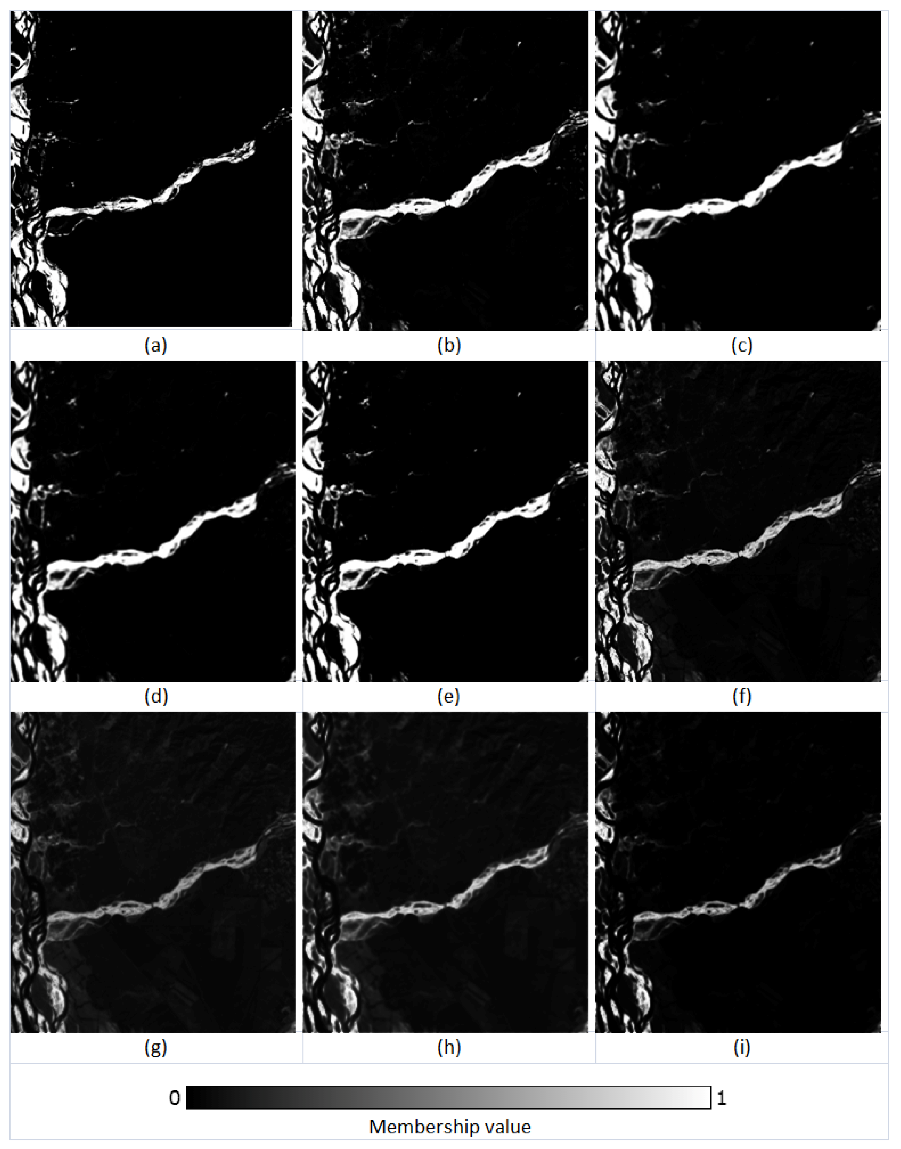
Figure 4.
The membership fraction (0–1) for the class ‘Dense Forest’ in (a) reference, (b) FCM output, (c) FCM-S output, (d) FLICM output, (e) ADFLICM output, (f) PCM output, (g) PCM-S output, (h) PLICM output, and (i) ADPLICM output.
Figure 4.
The membership fraction (0–1) for the class ‘Dense Forest’ in (a) reference, (b) FCM output, (c) FCM-S output, (d) FLICM output, (e) ADFLICM output, (f) PCM output, (g) PCM-S output, (h) PLICM output, and (i) ADPLICM output.

Figure 5.
The membership fraction (0–1) for the class ‘Eucalyptus’ in (a) reference, (b) FCM output, (c) FCM-S output, (d) FLICM output, (e) ADFLICM output, (f) PCM output, (g) PCM-S output, (h) PLICM output, and (i) ADPLICM output.
Figure 5.
The membership fraction (0–1) for the class ‘Eucalyptus’ in (a) reference, (b) FCM output, (c) FCM-S output, (d) FLICM output, (e) ADFLICM output, (f) PCM output, (g) PCM-S output, (h) PLICM output, and (i) ADPLICM output.

Figure 6.
The membership fraction (0–1) for the class ‘Grassland’ in (a) reference, (b) FCM output, (c) FCM-S output, (d) FLICM output, (e) ADFLICM output, (f) PCM output, (g) PCM-S output, (h) PLICM output, and (i) ADPLICM output.
Figure 6.
The membership fraction (0–1) for the class ‘Grassland’ in (a) reference, (b) FCM output, (c) FCM-S output, (d) FLICM output, (e) ADFLICM output, (f) PCM output, (g) PCM-S output, (h) PLICM output, and (i) ADPLICM output.

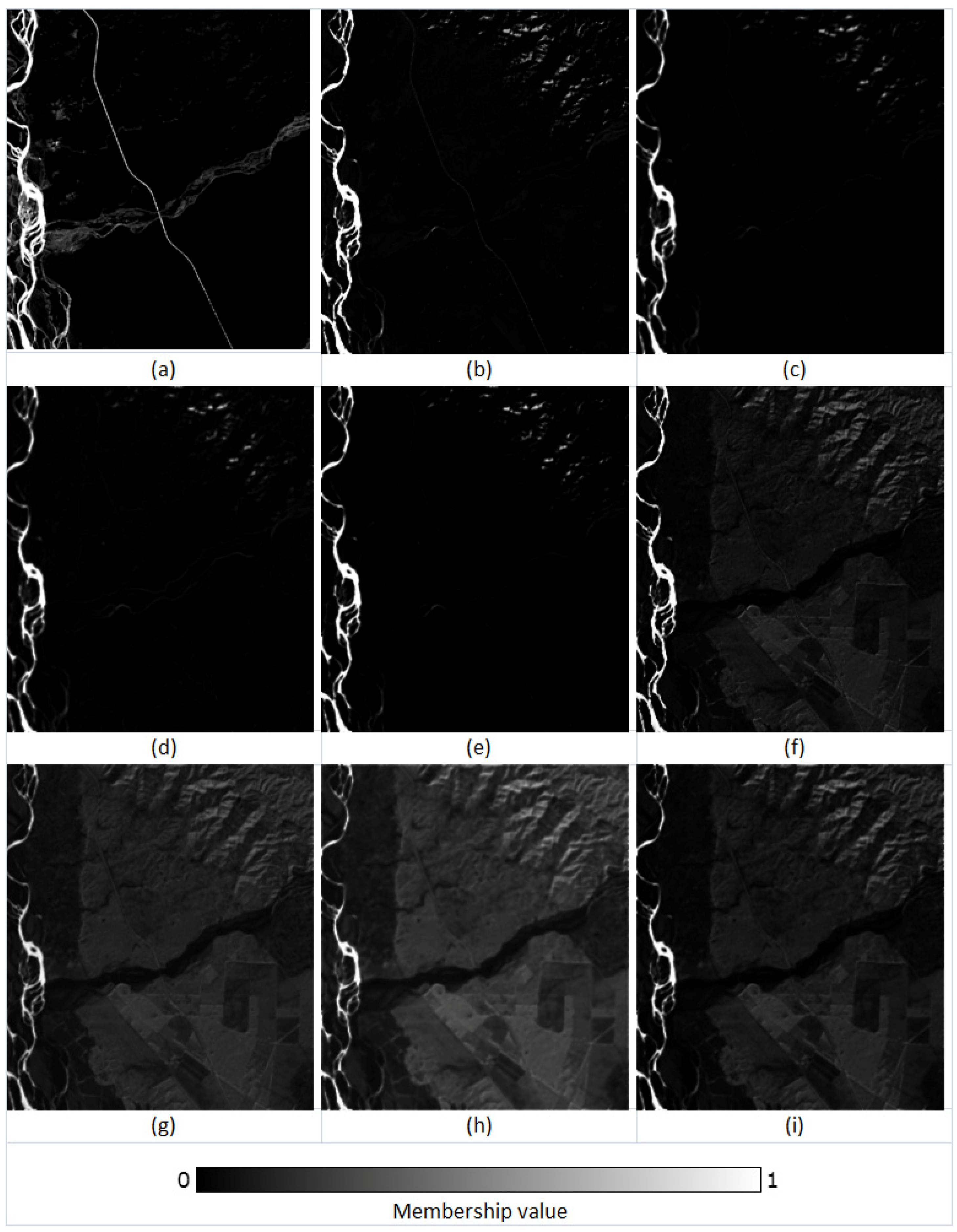
Figure 7.
The membership fraction (0–1) for the class ‘Riverine Sand’ in (a) reference, (b) FCM output, (c) FCM-S output, (d) FLICM output, (e) ADFLICM output, (f) PCM output, (g) PCM-S output, (h) PLICM output, and (i) ADPLICM output.
Figure 7.
The membership fraction (0–1) for the class ‘Riverine Sand’ in (a) reference, (b) FCM output, (c) FCM-S output, (d) FLICM output, (e) ADFLICM output, (f) PCM output, (g) PCM-S output, (h) PLICM output, and (i) ADPLICM output.

Figure 8.
The membership fraction (0–1) for the class ‘Water’ in (a) reference, (b) FCM output, (c) FCM-S output, (d) FLICM output, (e) ADFLICM output, (f) PCM output, (g) PCM-S output, (h) PLICM output, and (i) ADPLICM output.
Figure 8.
The membership fraction (0–1) for the class ‘Water’ in (a) reference, (b) FCM output, (c) FCM-S output, (d) FLICM output, (e) ADFLICM output, (f) PCM output, (g) PCM-S output, (h) PLICM output, and (i) ADPLICM output.

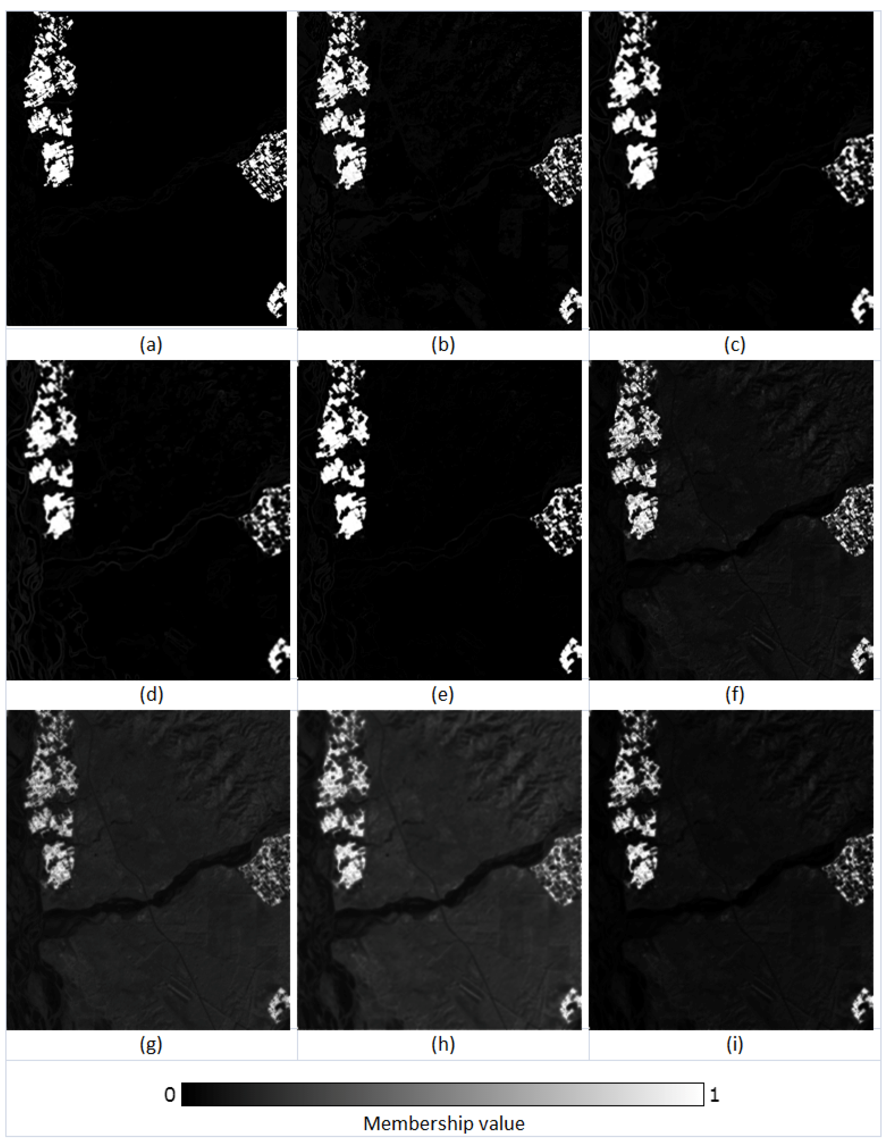
Figure 9.
The membership fraction (0–1) for the class ‘Wheat’ in (a) reference, (b) FCM output, (c) FCM-S output, (d) FLICM output, (e) ADFLICM output, (f) PCM output, (g) PCM-S output, (h) PLICM output, and (i) ADPLICM output.
Figure 9.
The membership fraction (0–1) for the class ‘Wheat’ in (a) reference, (b) FCM output, (c) FCM-S output, (d) FLICM output, (e) ADFLICM output, (f) PCM output, (g) PCM-S output, (h) PLICM output, and (i) ADPLICM output.

Figure 10.
FERM overall accuracy (in percentage) of classification algorithms when tested with different sample sets.
Figure 10.
FERM overall accuracy (in percentage) of classification algorithms when tested with different sample sets.

Figure 11.
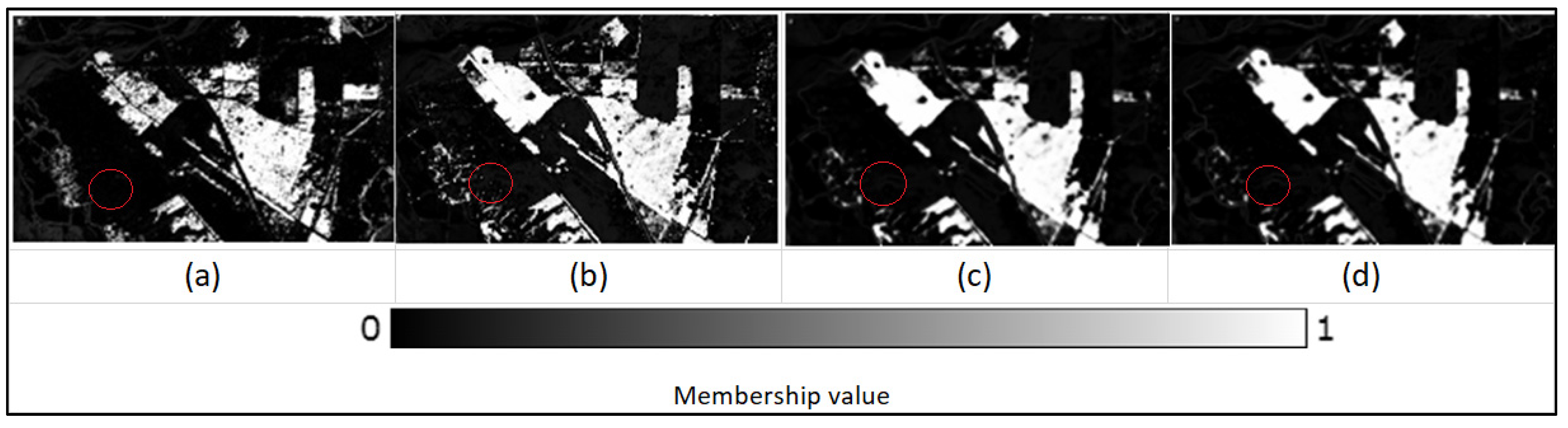
Example of fuzzy local spatial information classifiers in removing isolated pixels: (a) Reference fraction image for ‘Eucalyptus’ class, (b) FCM classifier output fraction image with isolated pixels, (c) FCM-S classifier output fraction image where isolated pixels are handled, and (d) FLICM classifier output fraction image where isolated pixels are handled.
Figure 11.
Example of fuzzy local spatial information classifiers in removing isolated pixels: (a) Reference fraction image for ‘Eucalyptus’ class, (b) FCM classifier output fraction image with isolated pixels, (c) FCM-S classifier output fraction image where isolated pixels are handled, and (d) FLICM classifier output fraction image where isolated pixels are handled.

Figure 12.
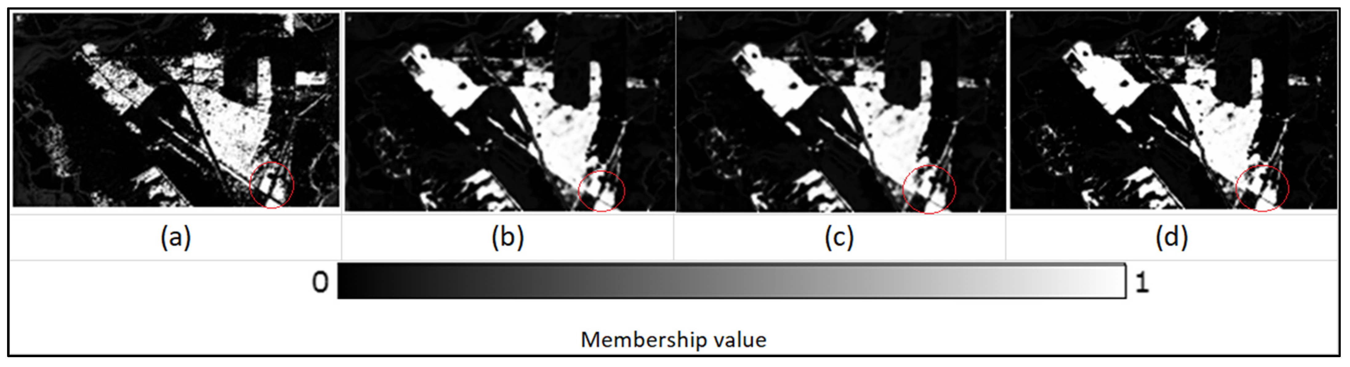
Example of fuzzy local spatial information classifiers in image detail preservation: (a) Reference fraction image for ‘Eucalyptus’ class, (b) FCM-S classifier output fraction image with vague edges, (c) FLICM classifier output fraction image with vague edges, and (d) ADFLICM classifier output fraction image with edges better preserved.
Figure 12.
Example of fuzzy local spatial information classifiers in image detail preservation: (a) Reference fraction image for ‘Eucalyptus’ class, (b) FCM-S classifier output fraction image with vague edges, (c) FLICM classifier output fraction image with vague edges, and (d) ADFLICM classifier output fraction image with edges better preserved.

Figure 13.
Global RMSE values for fuzzy local spatial information classifier outputs.

Figure 14.
Membership fraction (0–1) for the class ‘Riverine Sand’ generated by (a) FCM, (b) FCM-S, (c) FLICM, (d) ADFLICM, (e) PCM, (f) PCM-S, (g) PLICM, and (h) ADPLICM classifiers in the presence of untrained classes.
Figure 14.
Membership fraction (0–1) for the class ‘Riverine Sand’ generated by (a) FCM, (b) FCM-S, (c) FLICM, (d) ADFLICM, (e) PCM, (f) PCM-S, (g) PLICM, and (h) ADPLICM classifiers in the presence of untrained classes.

Figure 15.
Membership fraction (0–1) for the class ‘Water’ generated by (a) FCM, (b) FCM-S, (c) FLICM, (d) ADFLICM, (e) PCM, (f) PCM-S, (g) PLICM, and (h) ADPLICM classifiers in the presence of untrained classes.
Figure 15.
Membership fraction (0–1) for the class ‘Water’ generated by (a) FCM, (b) FCM-S, (c) FLICM, (d) ADFLICM, (e) PCM, (f) PCM-S, (g) PLICM, and (h) ADPLICM classifiers in the presence of untrained classes.

Figure 16.
Membership fraction (0–1) for the class ‘Wheat’ generated by (a) FCM, (b) FCM-S, (c) FLICM, (d) ADFLICM, (e) PCM, (f) PCM-S, (g) PLICM, and (h) ADPLICM classifiers in the presence of untrained classes.
Figure 16.
Membership fraction (0–1) for the class ‘Wheat’ generated by (a) FCM, (b) FCM-S, (c) FLICM, (d) ADFLICM, (e) PCM, (f) PCM-S, (g) PLICM, and (h) ADPLICM classifiers in the presence of untrained classes.

Figure 17.
Accuracy assessment results of the classifiers based on RMSE values.

Figure 18.
Global RMSE values of classifiers for different test datasets.

Figure 19.
The membership fraction image for the ‘Wheat’ class generated by (a) PCM, (b) PCM-S, (c) PLICM, and (d) ADPLICM algorithms.
Figure 19.
The membership fraction image for the ‘Wheat’ class generated by (a) PCM, (b) PCM-S, (c) PLICM, and (d) ADPLICM algorithms.

Figure 20.
Formosat-2 image corrupted with noise.

Figure 21.
The membership fraction image for the ‘Riverine Sand’ class generated by (a) FCM, (b) FCM-S, (c) PCM, and (d) PCM-S algorithms.
Figure 21.
The membership fraction image for the ‘Riverine Sand’ class generated by (a) FCM, (b) FCM-S, (c) PCM, and (d) PCM-S algorithms.


Table 1.
The parameter values optimized for the conventional classifiers and the local spatial information classifiers for supervised classification with all the classes.
Table 1.
The parameter values optimized for the conventional classifiers and the local spatial information classifiers for supervised classification with all the classes.
| FCM | PCM | FCM-S | PCM-S | FLICM | PLICM | ADFLICM | ADPLICM | |
|---|---|---|---|---|---|---|---|---|
| m | 1.7 | 1.8 | 1.5 | 2.2 | 1.7 | 2.2 | 1.5 | 1.8 |
| a | - | - | 2 | 0.5 | - | - | - | - |
| window size 1 | - | - | 3 | 3 | 3 | 3 | 3 | 3 |
1 Window size = 3 implies a 3 × 3 window around each pixel, making the number of neighboring pixels for each pixel to be 8 (i.e., NR = 8).
Table 2.
The overall accuracy (in percentage) of FERM obtained from the conventional fuzzy classification algorithms and fuzzy local spatial information classification algorithms.
Table 2.
The overall accuracy (in percentage) of FERM obtained from the conventional fuzzy classification algorithms and fuzzy local spatial information classification algorithms.
| FCM | FCM-S | FLICM | ADFLICM | PCM | PCM-S | PLICM | ADPLICM | |
|---|---|---|---|---|---|---|---|---|
| OA | 66.63% | 68.97% | 68.74% | 68.71% | 63.19% | 50.42% | 51.02% | 43.92% |
| OA1 | 83.04% | 84.51% | 85.31% | 84.08% | 76.42% | 62.88% | 66.79% | 61.67% |
| OA2 | 38.96% | 68.25% | 71.91% | 60.77% | 32.01% | 33.22% | 32.22% | 20.81% |
| OA3 | 69.82% | 56.46% | 53.03% | 62% | 72.71% | 49.12% | 47.73% | 40.09% |
Table 3.
Global RMSE values for fuzzy local spatial information classifiers.
| FCM-S | FLICM | ADFLICM | PCM-S | PLICM | ADPLICM | |
|---|---|---|---|---|---|---|
| RMSE | 0.230 | 0.239 | 0.230 | 0.254 | 0.297 | 0.281 |
Table 4.
RMSE values estimated on the outputs of different classifiers when supervised classification was applied in the presence of untrained classes.
Table 4.
RMSE values estimated on the outputs of different classifiers when supervised classification was applied in the presence of untrained classes.
| FCM | FCM-S | FLICM | ADFLICM | PCM | PCM-S | PLICM | ADPLICM | |
|---|---|---|---|---|---|---|---|---|
| Riverine Sand | 0.262 | 0.227 | 0.220 | 0.249 | 0.203 | 0.050 | 0.010 | 0.016 |
| Water | 0.356 | 0.336 | 0.338 | 0.358 | 0.358 | 0.216 | 0.276 | 0.243 |
| Wheat | 0.412 | 0.459 | 0.486 | 0.472 | 0.382 | 0.293 | 0.205 | 0.240 |
| Overall RMSE | 0.349 | 0.354 | 0.365 | 0.371 | 0.324 | 0.212 | 0.199 | 0.197 |
Table 5.
RMSE values of PCM-based classifiers for single class (‘Wheat’) extraction.
| PCM | PCM-S | PLICM | ADPLICM | |
|---|---|---|---|---|
| RMSE | 0.515 | 0.379 | 0.270 | 0.279 |
Publisher’s Note: MDPI stays neutral with regard to jurisdictional claims in published maps and institutional affiliations. |
© 2021 by the authors. Licensee MDPI, Basel, Switzerland. This article is an open access article distributed under the terms and conditions of the Creative Commons Attribution (CC BY) license (https://creativecommons.org/licenses/by/4.0/).
Share and Cite
MDPI and ACS Style
Madhu, A.; Kumar, A.; Jia, P. Exploring Fuzzy Local Spatial Information Algorithms for Remote Sensing Image Classification. Remote Sens. 2021, 13, 4163. https://doi.org/10.3390/rs13204163
AMA Style
Madhu A, Kumar A, Jia P. Exploring Fuzzy Local Spatial Information Algorithms for Remote Sensing Image Classification. Remote Sensing. 2021; 13(20):4163. https://doi.org/10.3390/rs13204163
Chicago/Turabian StyleMadhu, Anjali, Anil Kumar, and Peng Jia. 2021. "Exploring Fuzzy Local Spatial Information Algorithms for Remote Sensing Image Classification" Remote Sensing 13, no. 20: 4163. https://doi.org/10.3390/rs13204163
Note that from the first issue of 2016, this journal uses article numbers instead of page numbers. See further details here.