
Water Extraction in SAR Images Using Features Analysis and Dual-Threshold Graph Cut Model

1
Key Laboratory of Technology in Geo-Spatial Information Processing and Application System, Chinese Academy of Sciences, Beijing 100190, China
2
Aerospace Information Research Institute, Chinese Academy of Sciences, Beijing 100094, China
3
School of Electronic, Electrical and Communication Engineering, University of Chinese Academy of Sciences, Beijing 100049, China
4
The State Key Laboratory of High Speed Railway Track Technology, China Academy of Railway Sciences, Beijing 100891, China
*
Author to whom correspondence should be addressed.
Remote Sens. 2021, 13(17), 3465; https://doi.org/10.3390/rs13173465
Submission received: 9 July 2021
/
Revised: 25 August 2021
/
Accepted: 27 August 2021
/
Published: 1 September 2021
(This article belongs to the Section Remote Sensing Image Processing)
Abstract
:Timely identifying and detecting water bodies from SAR images are significant for flood monitoring and water resources management. In recent decades, deep learning has been applied to water extraction but is subject to the large difficulty of acquiring SAR dataset of various water bodies types, as well as heavy labeling work. In addition, the traditional methods mostly occur over the large, open lakes and rivers, rarely focusing on complex areas such as the urban water, and cannot automatically acquire the classification threshold. To address these issues, a novel water extraction method is proposed with high accuracy in this paper. Firstly, a multiscale feature extraction using a Gabor filter is conducted to reduce the noise and roughly identify water feature. Secondly, we apply the Otsu algorithm as well as a voting strategy to initially extract the homogeneous regions and for subsequent Gaussian mixture model (GMM). Finally, the dual threshold is obtained from the fitted Gaussian distribution of water and non-water, which is integrated into the graph cut model to redefine the weights of the edges, then constructing the energy function of the water map. The dual-threshold graph cut (DTGC) model precisely pinpoints the water location by minimizing the energy function. To verify the efficiency and robustness, our method and comparison methods, including the IGC method and IACM method, are tested on six different types of water bodies, by performing the accuracy assessment via comparing outcomes with the manually labeled ground truth. The qualitative and quantitative results show that the overall accuracy of our method for the whole dataset all surpasses 99%, along with an obvious improvement of the Kappa, F1-score, and IoU indicators. Therefore, DTGC method has the absolute advantage of automatically capturing water maps in different scenes of SAR images without specific prior knowledge and can also determine the optimal threshold range.
1. Introduction
Water resources have played an indispensable role in human agriculture and industrial production and life. Efficient monitoring of the distribution of water bodies can capture the attention of water resource managers for public health and safety (such as floods and pollution), water supply, tourism, etc. [1].
Recently, the remotely sensed data have been extensively utilized for the mapping of water. The optical image has a high resolution, capable of providing detailed and visible band information characteristics, which has been exploited for the water body extraction [2]. However, it is easily restricted by various night and weather factors, hindering the real-time acquisition of images, especially emergency tasks in severe weather conditions, such as the real-time monitoring of disaster areas [3], whereas synthetic aperture radar (SAR), such as a microwave active sensor, is unaffected by cloud cover, acquires images overnight, enables all-weather imaging [4], and has a wide range of observations. Therefore, drawing water mapping based on SAR images has garnered more attention from scholars recently [5,6]. Furthermore, the use of effective and relatively low-cost remote sensing technology to monitor floods and droughts can make a great contribution to the decision making and rescue action [5].
Currently, a variety of methods have been proposed to accurately map the extent of water and monitor flood changes from SAR images, which can be divided into two categories: deep-learning methods and the conventional methods. In recent decades, deep learning has made significant progress in water extraction, which is primarily based on optical images, as proposed in [1,7,8,9], but relatively little on SAR images [10,11], mainly because it is limited by the acquisition of high-quality SAR image dataset. For example, [11] used a dataset of 10 SAR images with a size of nearly 10,000 × 10,000 and cropped and expanded it to 21,180 images for training, verifying, and testing the dense depth separation convolution segmentation network, but it was time consuming for researchers to label such large amounts of data. Furthermore, the test sets and training sets should have the same size, meaning that large images need to be segmented in advance. Thus, in this article, we are committed to traditional methods for unsupervised water extraction over SAR images of any size and type.
Based on our summary, water surface mapping mainly includes the following basic algorithms: (i) threshold-based segmentation; (ii) region growing algorithm; (iii) texture feature-based method; and (iv) active contour model (ACM)-based method. However, the application of the above single algorithm has an inherent limitation. The threshold method is of simplicity and is computationally less time consuming, while it is easily affected by the image quality and the external environment, possibly resulting in misclassifications and holes. For large SAR data, the (ii) method has a heavy computational burden [12] and is limited by the seed point, with poor automation. Then, extracting the texture feature is often used for the preliminary identification in a series of processing chain, which is widely implemented in object-oriented methods by being combined with other algorithms, such as MRF, random forest, graph cut, etc. The process of ACM method is complex and time consuming, and the results are dependent upon the initial boundary conditions. Therefore, for mapping accurate water body information, the existing studies are more concerned about a combined application of multiple basic algorithms.
Du et al. [13] used the expectation-maximum (EM) algorithm to iteratively calculate the parameters of the Gaussian mixture model and combined with the graph cut model to extract the water surface. Leng et al. [14] applied the two-stage Otsu algorithm to obtain the initial contour line, and the regional ACM method was carried out in the narrow band to detect the edge of Poyang Lake, which was established at a certain distance from the initial boundary. Marcin et al. in [15] first performed watershed segmentation and then merged the segmented area into the output area of the river channel after selecting the seed point for optimizing the classification results. Sghaier et al. [16] proposed a method to identify rivers based on the local texture feature measurement and global knowledge related to the shape of the target object and the mathematical morphology. By using the tile-based thresholding to determine the initial boundary and the active contour model to refine the boundary, the heuristic and automatic water extraction (HAWE) method proposed in [17] was implemented to improve the accuracy of detecting the water from the Sentinel-1 SAR images. Evidently, the effective combination of algorithms contributes to the accuracy of water extraction.
However, to our knowledge, a large number of papers pay more attention to the exploration for large lakes [14,17,18,19,20,21], rivers [15,16], and the reservoirs [22,23], but few studies refer to the identification of water bodies in urban areas [8], which mainly includes urban rivers, ponds, small lakes, and fishing pools [1]. Li et al. [24] described a method of extracting complex urban rivers, but different subimage blocks had to be manually adjusted and selected for certain operations; therefore, there was a lack of automation. Mason et al. [25] used SAR images and LiDAR data to collect urban flood information semi-automatically, and only 76% of the water was correctly detected. Zeng et al. [26] adopted the optical image roughly to extract the water body with accuracy as high as 91%, which increased to the 94% through being rectified by SAR images. Automatically extracting the different urban water types only from a single SAR image is very challenging.
Specular reflection occupies a major position in water bodies, which indicates the reason for its low gray value and uniform texture characteristics. Generally, the uniformity is considered as the best feature for characterizing water surfaces, and it is conducive to the extraction of a large water area with a simple background. By contrast, small water bodies and low albedo non-water surfaces in urban areas may be confused by asphalt roads and shadows of buildings [27] because of a similar gray value but whose surface size is not large enough compared to that of water, along with strong spot response characteristics. In this context, the presence of speckle noise causes problems in extracting water [4], as well as impeding the accurate analysis of the SAR images. Through experiments, we find that every SAR image has a threshold for roughly identifying water bodies that are determined by analyzing the histogram of SAR image intensity [28]. Researchers have used the threshold solution methods, yet they rarely involve study areas with relatively little water surface, for the reason that the image histogram only displays one prominent peak [28]; therefore, finding the threshold is difficult. For all the above reasons, it becomes especially hard to identify the multiple water types across complex scenes. Moreover, in most traditional methods, the extraction extent is relatively narrow, being only applicable for distinguishing one type of water.
To deal with the mentioned problems, this paper proposes a novel water extraction algorithm using SAR images. First, the Gabor filter is employed to produce texture feature maps, which are binarized by the Otsu algorithm, and then an initial image segmentation with voting strategy is generated. Second, we calculate the initial segmentation map as GMM parameters for estimating the probability distributions, such that the dual threshold is derived from them. Finally, the proposed dual-threshold graph cut (DTGC) model is implemented on the SAR images to obtain water segmentation results. Such a combination of multiscale texture features and the DTGC model can not only locate the optimal threshold range through a dual threshold but also extract various water types, as well as assist long-term water monitoring.
The rest of this paper is organized as follows: In Section 2, the related theories of the proposed method are discussed in detail. Section 3 presents information about the dataset and experimental results. The qualitative and quantitative discussion for results is provided in Section 4. Finally, the conclusions are discussed in Section 5.
2. Materials and Methods
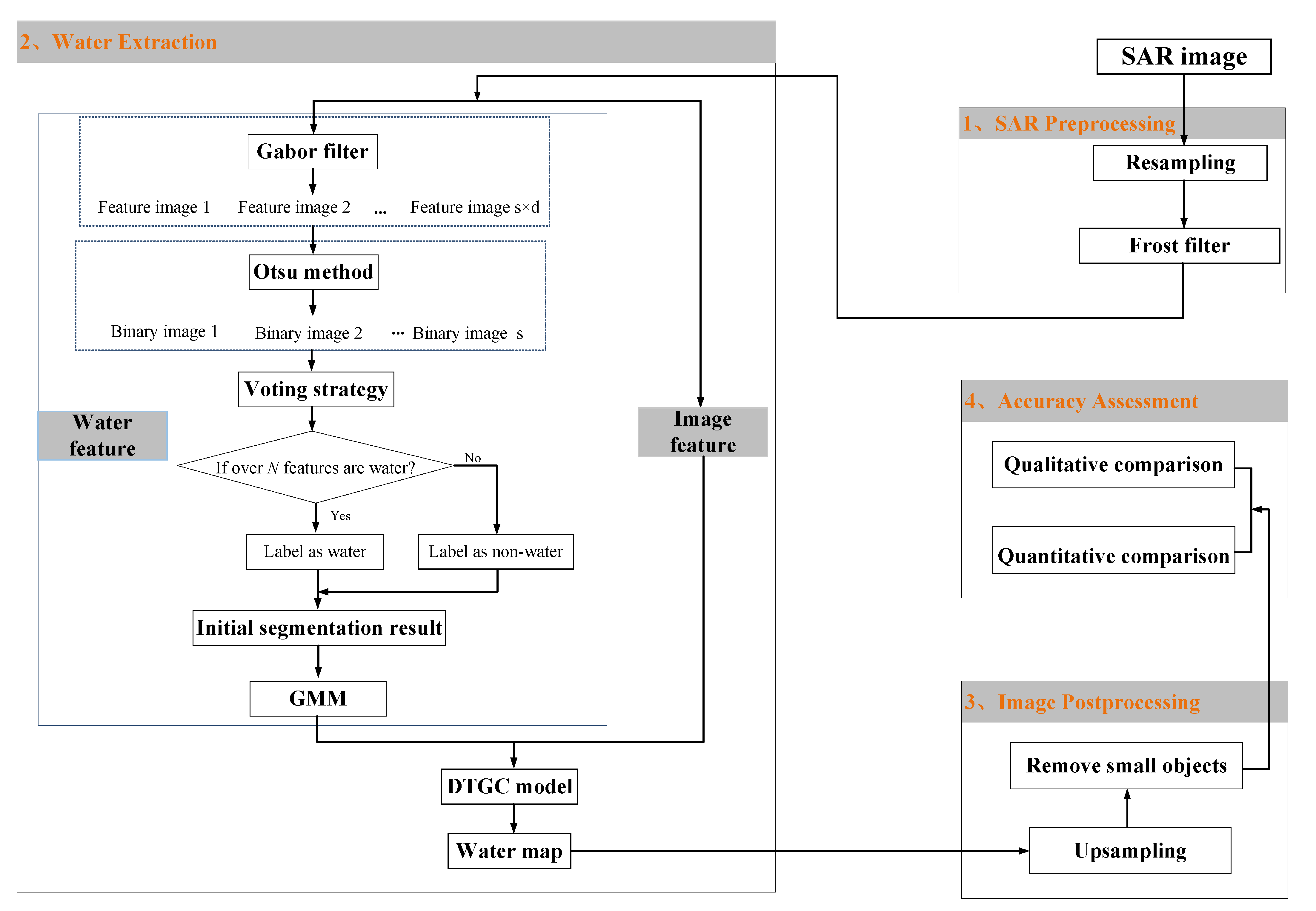
An overview of the proposed approach is presented in Figure 1. It is primarily divided into the following four parts: image preprocessing, water extraction, image postprocessing, and accuracy assessment. In the image preprocessing part, it includes image resampling and a Frost filter. The purpose of resampling is to fasten the running speed of the proposed framework while making the water feature more concentrated, and the Frost filter is used to suppress the speckle noise. In the second part, we employ the Gabor filter to analyze the texture characteristics of the water body and the proposed DTGC algorithm to acquire the whole water area. In the third step, when the water body extraction is completed initially, performing upsampling to restore the original image size; at the same time, some isolated, small non-water targets are corrected or removed through postprocessing. Finally, we qualitatively and quantitatively compare the accuracy of all methods by using different test data to validate the effectiveness and universality of the DTGC model.
2.1. Image Preprocessing
2.1.1. Image Resampling
We use the nearest-neighbor interpolation method to resample the image in this article, the purpose of which is to resize the SAR image and enhance the image segmentation speed. The specific formula of the resampling is shown in (1):
Equation (1) represents the resampling for the SAR image by times. The choice of parameter , which belongs to [0,1], is essential to the result, possibly leading to a significant reduction of useful information if biased. In addition, resampling results in a reduction in spatial resolution, which becomes times that of the original resolution. However, when the image data are large, the scaled-down images have the advantage of increasing the sensing range while reducing the amount of calculation, making it more convenient to concentrate on the extraction of water features. In addition, the quality of image segmentation can be further improved upon subsequent experiments.
2.1.2. Frost Filter
The SAR images are highly suppressed by the coherent speckle noise. Therefore, this paper applies the Frost filter to reduce the influence of speckle noise and make the histogram show obvious peaks and troughs for study areas with relatively little water by combining them with resampling, which are only displays one prominent peak [28]. The Frost filter function [29] is defined as below:
where is the position of the current pixel, represents the output of the filter, the represents the pixel value in the window centered in , is a regulator, is a variant coefficient defined by the ratio of sample standard deviation and sample mean, and is the distance between any pixels in the current window to the central pixel [29].
2.2. Water Extraction
For the previous methods, apart from the single objective, it also has the inability to obtain the best threshold for detecting any type of water bodies. Herein, a novel method is designed for segmenting the water areas from a single SAR image, as well as overcoming the difficulties in extracting water bodies over complicated SAR image scenes. The DTGC model is improved based on the theory of graph cut [30], by using a dual threshold to redefine the weights of the graph cut model edge, and constructs the energy function of the water map in accordance with the water feature and image feature. The flowchart of the water extraction method is shown in Section 2 of Figure 1.
We employ the Otsu algorithm to binarize the multiscale feature images generated by Gabor filter. In addition, the initial segmentation image obtained by the voting strategy is explored for calculating the GMM parameters. Then, the probability density of the pixels being water and non-water bodies is taken as the water feature, while the image feature comprehensively considers the relationship between the gray value and spatial position of the pixel neighborhood. Under the combined application of these, the proposed method minimizes the energy function of the graph and directly obtains the accurate water map information.
2.2.1. Water Feature
For the large area of water surface, Gaussian distribution assumed is suitable for fitting its image intensity histogram, which contains two partially overlapped distributions of water and non-water pixels [28]. In addition, the segmentation threshold can be easily computed by their intersection, whereas, with regard to the SAR images with relatively small water, the optimal threshold is difficult to acquire due to the not prominent troughs. Thus, we utilize two Gaussian distributions to fit the distribution of water and non-water pixels, constituting the Gaussian mixture model (GMM), whose parameters are obtained under the combined application of the Gabor filter, Otsu method, and voting strategy. Then, the Gaussian probability of the pixels being water and non-water is considered as the water feature.
First, the Gabor filter is applied to capture the texture features. The Gabor filter is a complex sine function that is modulated by a Gaussian envelope, which has been widely used in the computer vision and image-processing fields [31]. The filter used in this study is even a symmetric Gabor filter [31] for providing detailed features of different scales and directions with form:
The parameters are further specified in Equation (4):
where is the direction of the Gabor filter kernel; is the standard deviation of the Gaussian envelope, which determines the scale of the Gabor filter; and represents the number of scales and directions, respectively; and denotes the ellipticity of the Gabor function [31].
In the entire paper, the scale of the Gabor filter is set to 5, and the direction is set to 6, setting to for refining texture features. Then, this generates a multiscale and multidirectional feature set , which has been normalized.
Second, the Otsu method is applied to binarize the texture feature set. With the purpose of extracting the most representative features, we employ the maximum method to fusing the multidirectional intermediate images instead of using all features, then obtaining the fusion image that is composed of the largest feature values of pixels at each scale, which is defined as:
To maximize noise rejection and retain the image information, we binarize the fused image of each scale by the initial threshold , which is delivered by the Otsu algorithm [32], for capturing the most obvious feature of pixels. In this way, the optimal feature map for each scale is calculated as:
Generally, due to the speckle noise interference, the optimal threshold must be smaller than the threshold obtained from the original image. Hence, such a pixel tends to be water when ; therefore, the feature values of pixels satisfying this condition are set to 1. By contrast, if the pixels meet the given condition that , these pixels are more possible to belong to the background, whose feature values are set to 0. After that, the optimal feature maps of five scales are presented.
Third, we adopt the voting strategy for the final feature map. Five feature maps are produced by the above processes, of which each pixel contains five features, water or non-water. Therefore, the voting strategy in [33] is introduced to get the final segmentation image instead of averaging.
If the sum of pixel features considered that water is greater than or equal to a feature threshold , the corresponding pixel is tentatively determined as water that is given the value 1. Otherwise, the value 0 is given. The changes with different SAR images, whose range is [1,5], generally 3 or 4. The binarized initial segmentation image is obtained after a series of operations above.
Then, we establish the Gaussian mixture model (GMM). Usually, GMM parameters are estimated by the EM algorithm [34], while requiring continuous iterations to arrive at the optimal value, which takes a long time for large images and lowering accuracy. Therefore, the proposed method utilizes the initial segmentation map obtained by voting strategy to calculate the expectation , variance , and weight of foreground and background as GMM parameters, rather than EM method. Collection of the parameters is described as below:
where . The probability density distributions of water () and non-water () are computed by using Equation (8) [35]:
At last, the energy function of the water feature can be expressed as Equation (9) [36]:
where represents all pixels in the image, and the label of indicates whether it is water (fg) or non-water (bg). The cost of assigning a label to the pixel is specified by Equation (10):
2.2.2. Image Feature
We integrate the image feature into the energy function according to the paper [36]. The image feature links the amplitude information and the spatial position information of the pixel neighborhood, measuring the similarity between neighboring pixels pairs.
The energy function of the image feature [36] is as follows:
where and represent the image amplitude value of the adjacent pixel and , indicates all pairs of neighboring pixels, correspondingly, and denotes the Euclidean distance of them, along with meaning the average value of all neighboring pixel pairs of the entire image.
2.2.3. DTGC Model
Dual-Threshold
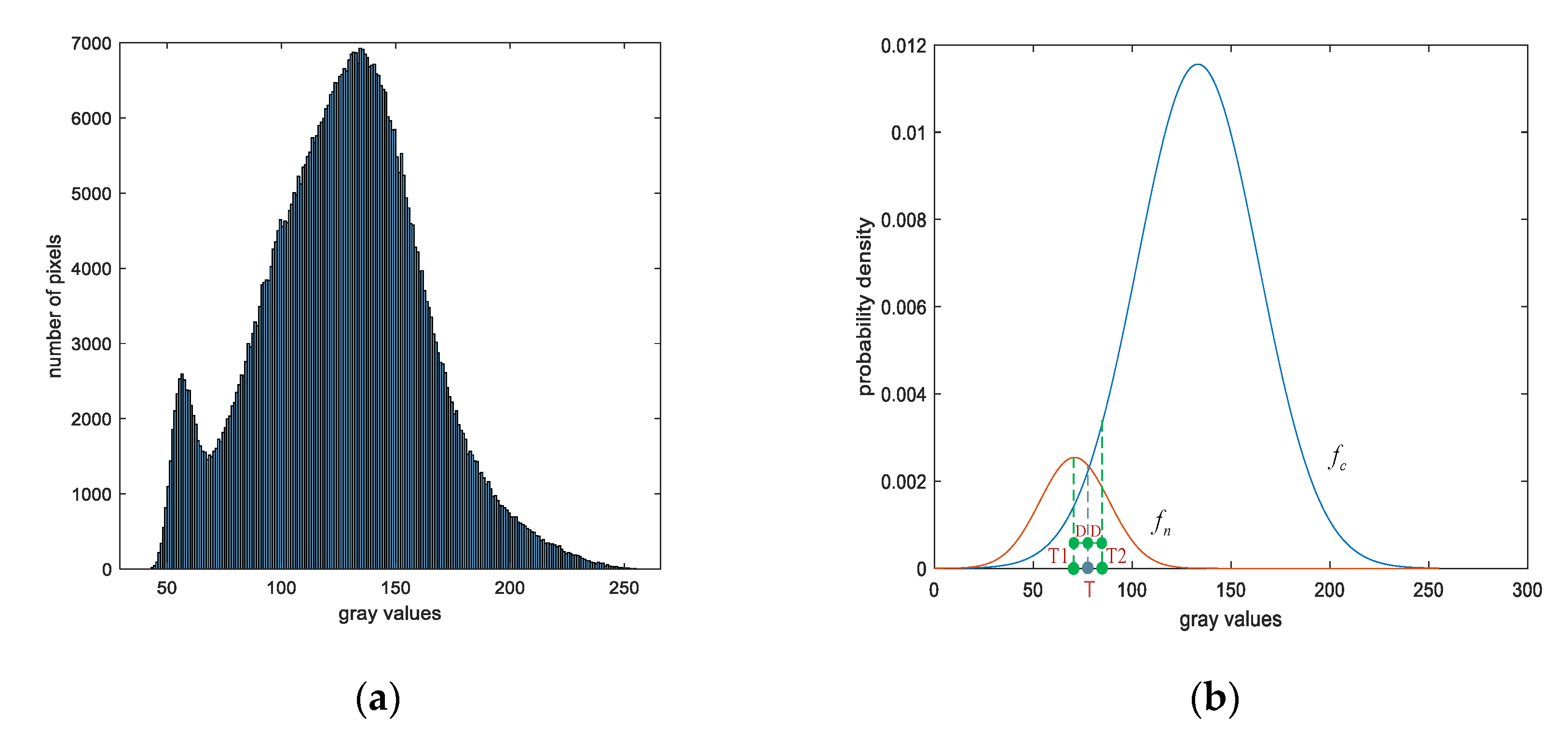
An example used for analyzing the fitting effect of GMM in this section is shown in Figure 2. Figure 2a is the gray histogram, and the probability distribution curves of each gray value belonging to water and non-water are and , respectively, which are further illustrated in Figure 2b, where the GMM properly fits the gray histogram trend of the SAR image.
It is observed that the distribution curves in Figure 2b intersect at the pixel value . Supposing that the is used as the threshold for segmentation, fractured boundaries and voids may occur. Therefore, inspired by the , a dual threshold is introduced to retain edge information.
We first set the threshold range [,] near , as shown in Figure 2b, and the formula is given by (14).
where indicates the distance between and or and is defined as:
The coefficients 0.5 in Equation (15) are the best value selected through numerous experiments, which can be changed according to requirements. The and are from Equation (7).
Energy Function
This paper constructs the energy function by establishing the water feature () and image feature (), and it serves:
where , ranging from 0 to 1, is the weighting coefficient for balancing the relative relationship between the image itself and its neighborhood. If multilook processing is performed, it can increase the parameter to improve the accuracy of the results.
Graph Construction
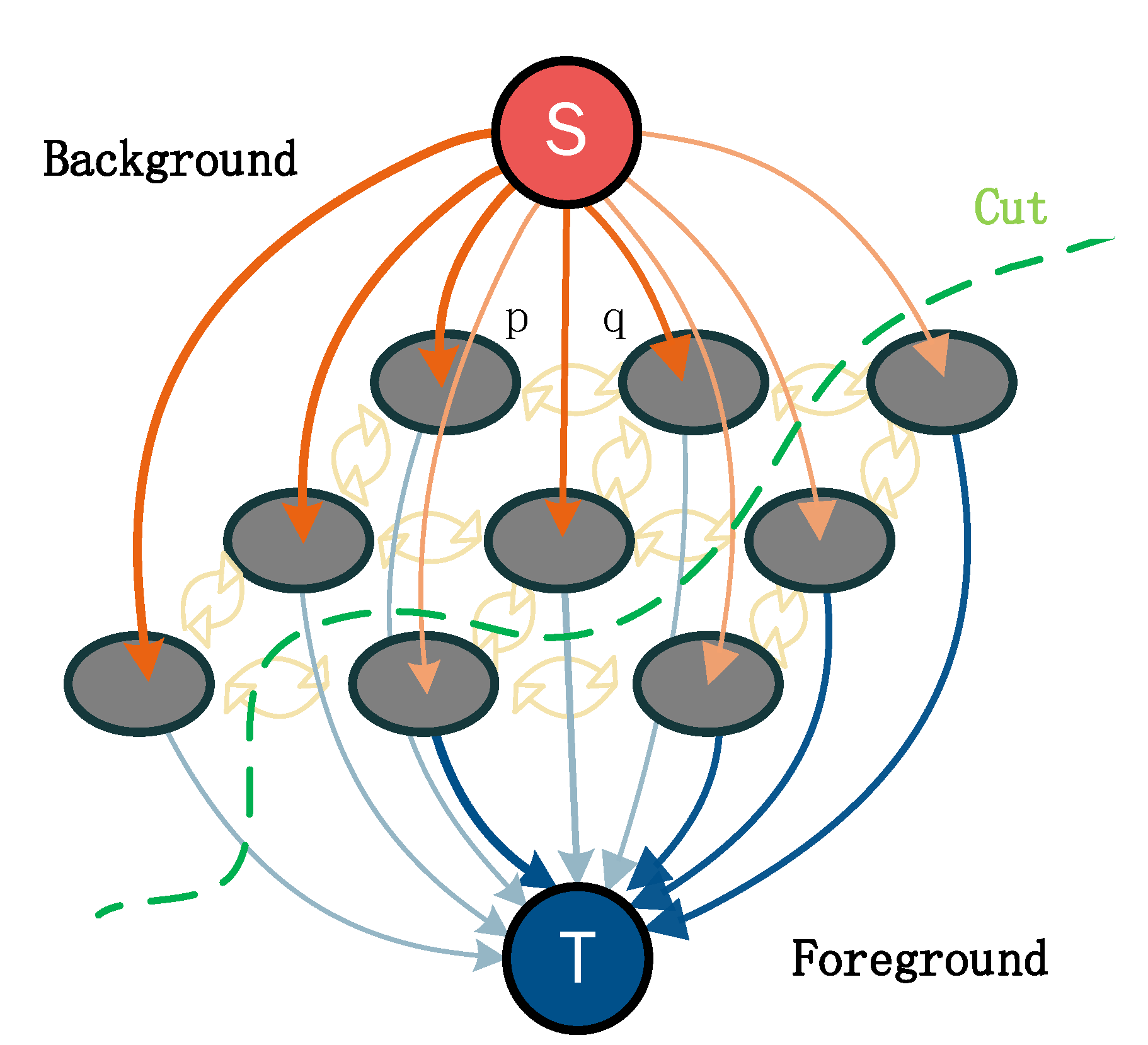
Next, according to [36], we create a graph for a single SAR image, including nodes and edge sets , as demonstrated in Figure 3 and Equation (17).
The nodes contain two different types, which are terminal nodes and pixel nodes. The former includes source and sink that, respectively, represent the background and foreground of the image. In the latter, each pixel represents a node. The is set as suggested in [36]:
In addition, there are two kinds of edges in the , namely, the neighbor connecting edge and the terminal connecting edge . The eight-neighborhood pixel of the pixel forms an , and each pixel is connected to the foreground and the background ; therefore, the edge and constitute the edge . The weights of and are related to the image feature and water feature potential separately.
Weight Setting
In this work, we improve the weight setting method in [36] by combining the dual threshold for better classification performance, with the edge weight type and its weight setting conditions depicted in Table 1 that are based on the following ideas:
- For , similar pixels should be assigned higher weights, whereas obviously different pixels are given lower weights [37].
- For , the edge weights are further restricted by the dual threshold. A detailed analysis of Figure 2b, when , the probability of the gray value on the curve surpasses more than 1 time of which on the , showing that the possibility of pixels belonging to the foreground is very low. Thus, to ensure that the minimum cut acts on the edge , the edge weights of pixels that meet the above given condition are assigned as 0. In a similar way, for the case of , the probability of pixels being water is slightly greater than that of non-water. Specifically, because of the water body generally of a low gray value, the pixels fulfilling the above conditions have a greater chance of being water; therefore, the weights of the edge are set to 0.
- For , supposing that the edge weights between the interval [,] and [,] are still serving as the Gaussian probability, the boundary of water and non-water sometimes would become blurred. Therefore, the weights are set to and allow the maximum flow to pass. The definition rule of is in Equation (19):
Energy Minimization
Dealing with the problem of the minimum cut of the graph is finding the minimum loss of the cut [38], which partitions the nodes into two disjoint parts: water and non-water. The cut is as follows:
where is the weight of edge , which belongs to a cut of Graph , and denotes the set of all cuts. The new min-cut/max-flow algorithm presented in [37] is employed for energy minimization in this paper.
2.3. Postprocessing
After adopting the DTGC model, pixels are successfully classified into two categories: water and non-water. However, the ships have brighter pixels that occur within the detected objects, which may lead to several small gaps. Additionally, thresholding always suffers from the noise that often exists in confounding the environment of SAR images [10], in terms of obscured buildings, road shadows, small non-target water, as well as mountain shadows, etc., making the separation of these objects from the results difficult.
As a consequence, for delineating the extent of the water from SAR images completely, it is necessary to postprocess the extraction results that are achieved by the DTGC model. The procedure is mainly divided into three parts: (1) The nearest-neighbor interpolation algorithm is still applied to complete upsampling to restore the original image size; (2) it needs to fill gaps caused by ships or sand; and (3) we determine the minimum ratio of the bounding rectangle to its area [13] along with setting the minimum area threshold [16] for eliminating small patches of non-targets. The third step is mainly because the water bodies are characterized by irregular shapes, whose area is usually smaller than the area of its smallest circumscribed rectangle. However, regarding the above noise, the difference is relatively small, meaning that the object is removed in the case that its area is smaller than or close to its smallest circumscribed rectangle area.
2.4. Accuracy Assessment
To gain a deeper insight into the performance of the DTGC algorithm, we made the manually labeled results based on Google Earth as the ground truth and compared our method with two typical methods, namely, improved graph cuts (IGC) [13] and improved ACM (IACM) [14]. For comprehensively measuring the accuracy of the three methods over the ground truth, the comparison is divided into two parts, one containing the qualitative comparison by visual inspection on results with different water types and another for quantitative evaluation by taking six evaluation metrics, pixel by pixel, including the overall accuracy (OA), the precision (Pre), the recall (Rec), the Kappa coefficient (Kappa), the F1-score, and the intersection over Union (IoU) [9]. These metrics are defined as follows:
where TP, FP, TN, and FN denote the true positive, false positive, true negative, and false negative pixels, respectively [10]. P is the total number of image pixels, and . In theory, the high precision and recall rate indicate a low commission and omission error. Simultaneously, the Kappa, F1-score, and IoU indexes are the comprehensive indicators of evaluating the entire performance of a method [1].
3. Results
3.1. Study Area and Dataset Description
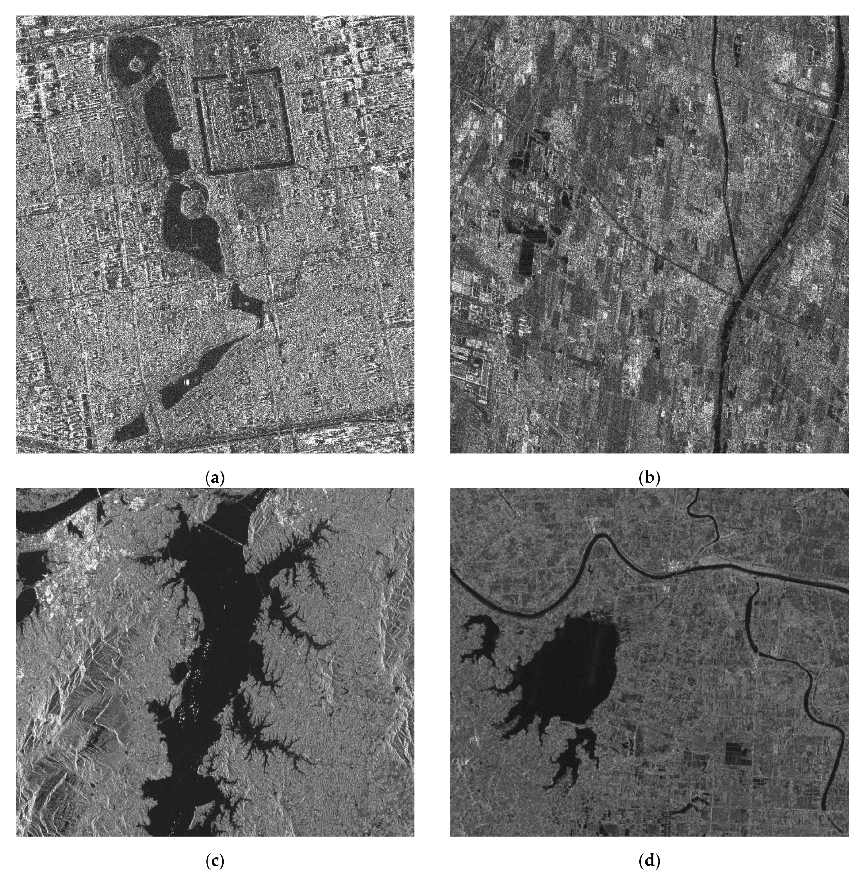
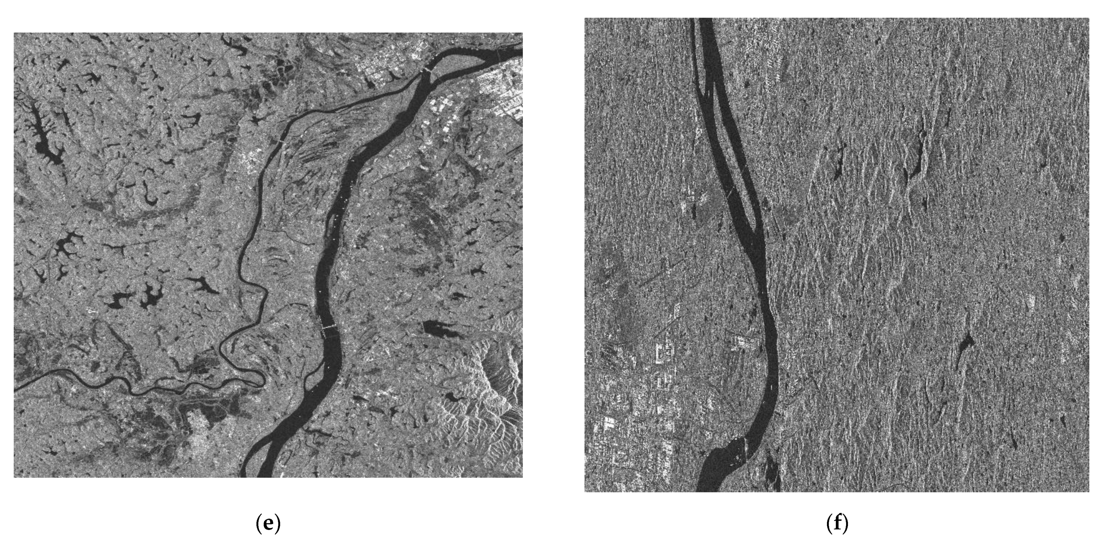
Within the study, the water bodies of the six regions under the complex and changeable environment were selected to test the performance of the proposed method, mainly relating to urban water, lakes and rivers, etc. The dataset is, respectively, from the satellites of TerraSAR-X (3 m resolution), GF-3 (3 m resolution) and Sentinal-1 (10 m resolution). The GF-3 and TerraSAR-X use the raw SAR intensity image with the preprocessing in Figure 1, and only the Sentinel-1 data are performed by terrain correction, which does not affect the experimental results. Our method is applicable to any kind of SAR intensity images. The specific data information is given in Figure A1 of Appendix A and Table 2.
3.2. Experiment Results
In this experiment, three classification methods, which are the proposed method, IGC method, and IACM method, were tested on six SAR images of different scenes and different satellites. Moreover, for further thorough analysis, in addition to the results of the three methods, the parameter setting for each image is also shown, as well as the detected texture feature maps.
3.2.1. Parameter Setting
In terms of objectively evaluating the results of water extraction and ensuring the authenticity and reliability of the comparison experiments, the same pretreatment is employed on all the methods. According to the Section 2.2.1, the scale of Gabor filter is 5, the direction is 6, and ellipticity is set to ,which are the determined parameters and do not change with the images. In addition, the setting of some parameters obviously influences the comparison results, which involve the resampling factor , the energy function coefficient of the DTGC model, the energy function coefficient of IGC model in [13], and the number of iterations in [14].
The data of the following parameters are all the optimal results that come from the continuous experimentations, as well as trial and error, which are listed in Table 3.
In addition, then we use the equivalent numbers of looks (ENL) [39] to evaluate the effect of resampling and Frost filter in preprocessing. Table 4 shows the comparison between the original image and the denoised image. The higher the ENL value, the higher the smoothing efficiency of the speckle noise in the uniform area [39]. It can be seen from Table 4 that the preprocessing can effectively reduce noise interference, especially in urban water bodies.
3.2.2. Feature Extraction Results
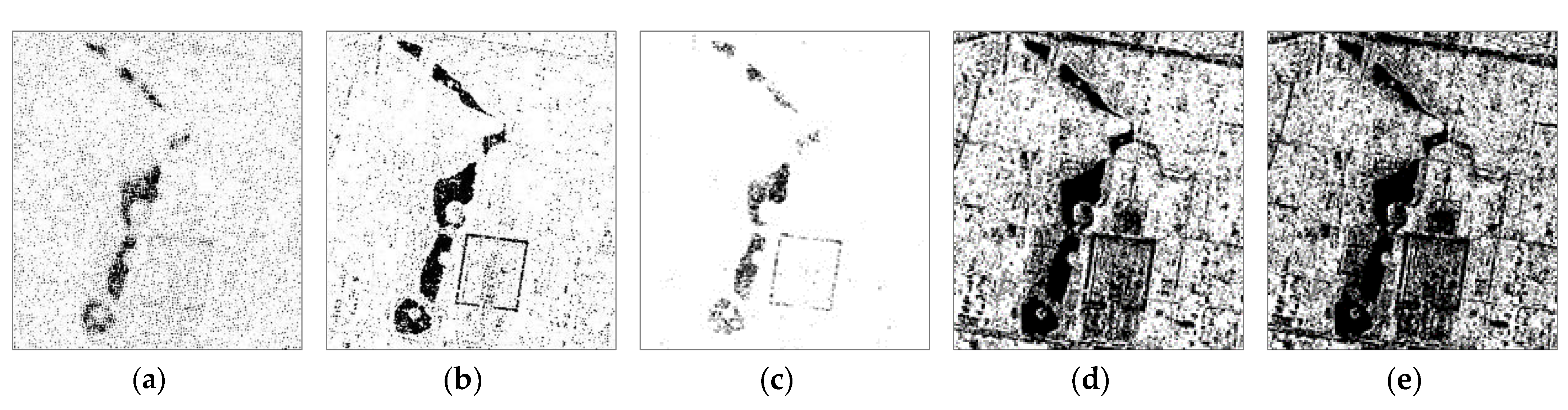
Taking Data A as an example, the binarized images of five scales containing black pixels (water area) and white pixels (non-water area) are generated by the Otsu thresholding method, as presented in Figure 4. Additionally, parallel operation was taken in this article to increase the running speed.
In Figure 4, we note that all scales of the water features are extracted, wherein, the feature map in scale 2 gives the preferable result, but the edges are fractured to varying degrees. The noise is the least in the scale 3, albeit with a large number of missing targets. Meanwhile, the optimal scale for different data is not uniform. Thus, in this situation, for ensuring the integrity of the water surface, the best choice is to employ a voting strategy rather than manually selecting the optimal scale from all feature maps.
Next, Figure 5 exactly reveals the initial segmentation results acquired by a voting strategy over all data, which are responsible for providing more accurate parameters for the subsequent GMM. In observing Figure 5a, compared with the map of scale 2, even though the noise has increased, it does not affect the recognition for the basic outline of the water body. Therefore, the voting strategy has been also applied to other data.
3.2.3. Proposed Method and Comparison Methods Results
The GMM parameters of each image are calculated from the initial segmentation maps in Figure 5 and then along with integrating the proposed DTGC model for the accurate water area classification. Finally, with setting the parameters according to 3.2.1, the results of our method and comparison methods across the whole dataset are given in Figure 6, where the omission error and commission error are also displayed, labeled green and red separately.
4. Discussion
To confirm the feasibility and robustness of our method, the following three aspects are comprehensively explored. In Section 4.1, the extraction outcomes of all methods for different water types are qualitatively analyzed. In Section 4.2, evaluation indicators in Section 2.4 are used to quantitatively compare the proposed method with other methods. In Section 4.3, we compute the running time of the dataset for comparing the algorithm complexity.
4.1. Qualitative Comparison for Different Water Types
In this section, visually, we compare the overall performance of these methods on all different test sites. It can be intuitively seen in Figure 7 that the classification results of three methods are different. On the whole, all algorithms perform better throughout obvious and clear water bodies, such as large lakes, rivers, and urban lakes. However, in comparison with the IGC and IACM method, the DTGC method gives the most favorable results in detecting urban water bodies surrounded by a complex environment in Data A and Data B, which are also the main targets in this paper.
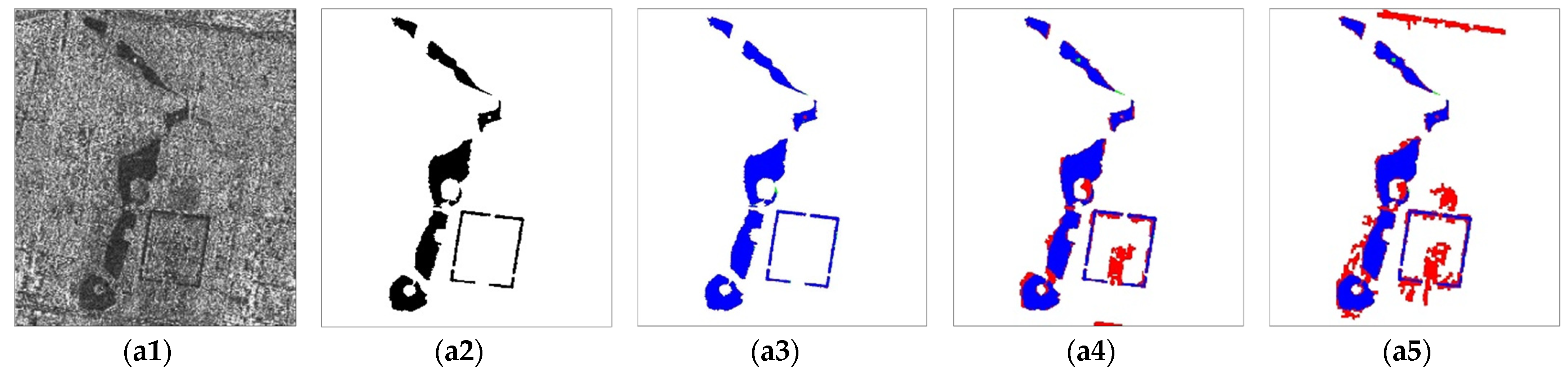
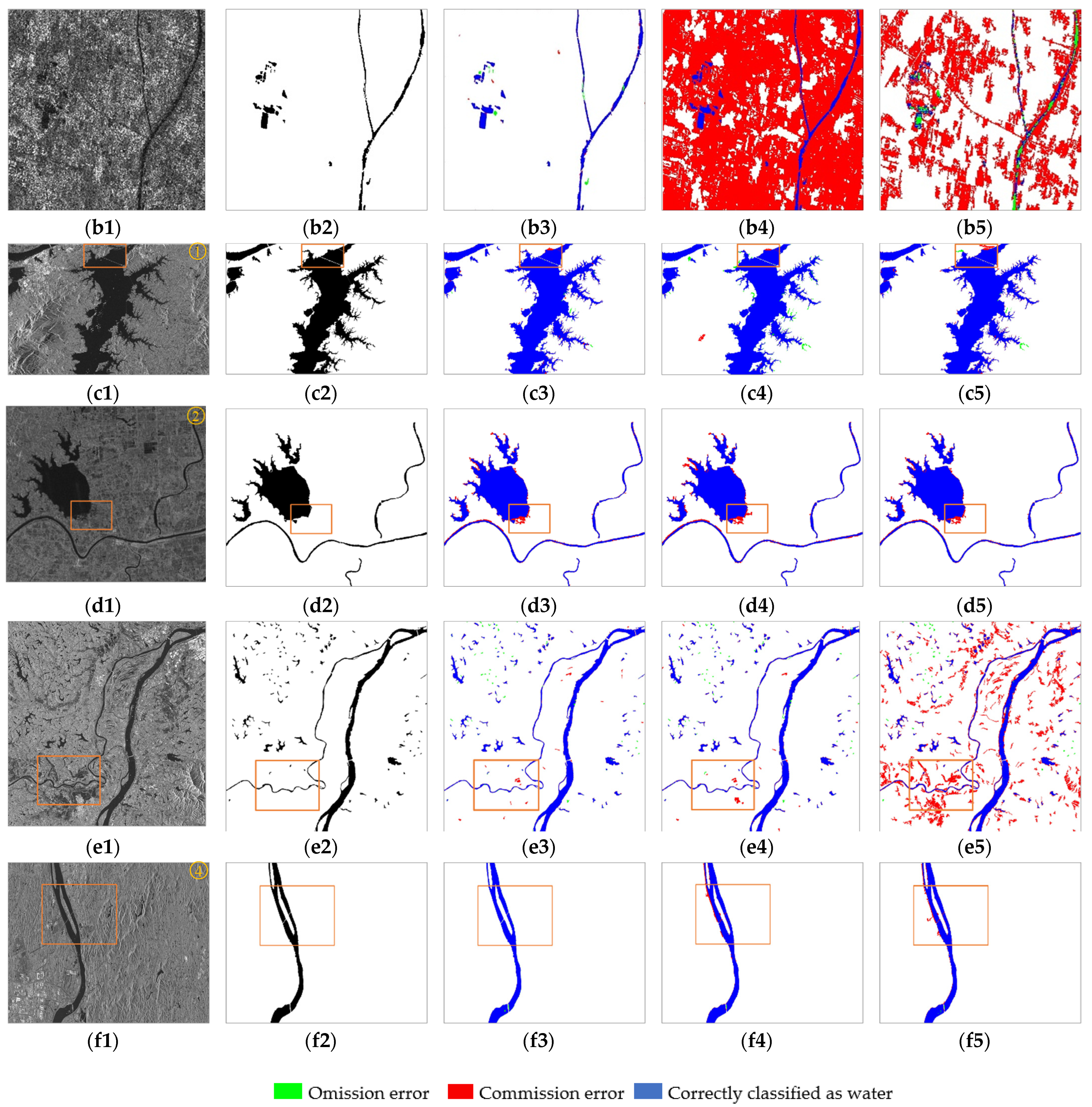
From Figure 6 (a1–a5), we can see that all methods can identify slightly larger lakes, but the comparison methods perform worst in the boundary information, both of which have serious errors in the rivers around the Forbidden City. In the case of relatively less water surface in Figure 6b, both the IGC and IACM methods are affected by noise, such that they wrongly detect a large number of dense buildings and roads as water, with fuzzy boundary information, whereas, in Figure 6 (b3), we find that the outcome of our method is quite accurate.
The urban water is not obviously visible in the SAR image due to dense urban buildings, etc.; therefore, it becomes difficult to identify any significant water pixels only by pixel-based processing. Although our method can refine the boundaries as well as suppressing noise to a certain extent, it still has the omission and commission error.
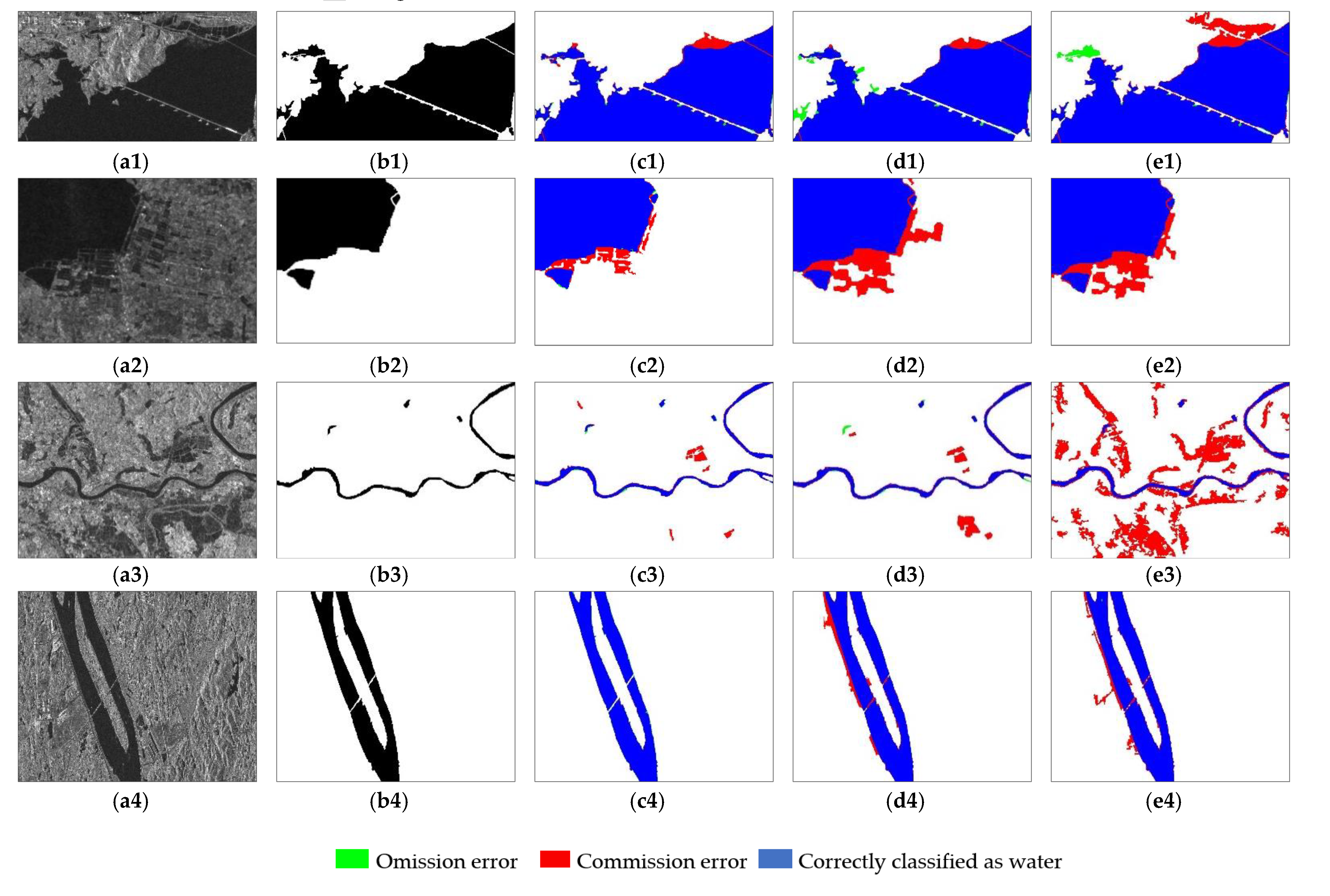
The results of Data C–F demonstrate a notable improvement over the three methods in detecting the overall outline of open lakes and rivers, yet with some discrepancies between them, as shown in Figure 7, where the enhancement in four zoomed-in regions ①–④ of Figure 6 is further visualized.
Regarding the first line images in Figure 7, the reason of the largest discrepancy occurring in the top-right corner is that the IACM method incorrectly identifies the buildings as water. Moreover, the three methods have varying degrees of omission errors. Upon visual inspection for the results of the site ②, all methods have the false-alarm errors, which are most severe in the IGC method. In addition, only our method and the IGC method can extract most small water bodies without being disturbed by the noise in Data E. As for the wide river Data F, where there are few buildings and other interference objects, it can be clearly visualized that all methods perform notably well in distinguishing the target and the background. The orange boxes in Figure 6e,f reveal the regions of commission errors at the water boundary that are eliminated in the DTGC result, as can be further seen in Figure 7 (d3,e3), where the comparison methods have an overdetection, especially the IACM method. Moreover, another interesting result for site ④ is that the comparison methods all divide the riverbank into a water area by mistake, because both classes have similar gray values.
In conclusion, the classification outcomes for all tested methods in Figure 6 and Figure 7 suggest that the proposed method can adequately capture the water-cover region, noting that the effect in extracting open water and small water areas is also not inferior to the contrast methods. Furthermore, the IGC and IACM methods contain more meaningless noise caused by urban buildings and other non-water objects. In addition, the accuracy of three methods is further quantitatively discussed in Section 4.2.
4.2. Classification Accuracy Results of Three Methods
To measure the overall performance of the DTGC model over the whole test set, this paper calculated the evaluation indexes in Section 2.4, based on the water maps extracted by the three methods and the ground truth. Table 5 summarizes the accuracy on six test areas for all methods.
With regard to the urban water extraction, the statistics indicate that the proposed method achieves a high accuracy, with the precision of Data A and Data B at 96.26% and 89.03%, and the Kappa, F1-score, and IoU indicators are all over 0.9, with absolute advantages. Furthermore, for Data B, both the IGC and IACM methods perform poorly, erroneously classifying a large group of buildings as water with precision as low as 3.2% and 4.4% separately. In Data A, the comparison methods perform slightly better, with IoU at 0.721 and 0.554. The water that is not completely detected by the two methods is because the estimation of GMM parameters and initial boundary leads to bad decision making. In contrast with the comparison methods, by considering multiscale texture features, the DTGC approach can obviously suppress the noise as well as achieve a satisfactory classification result, showing as much as a 33% overall accuracy enhancement and more for other indicators.
The areas in Data C–F cover relatively few dense buildings around lakes and rivers; therefore, the division accuracy of the comparative methods has been improved significantly, with a lower commission error, all less than 3%. Moreover, when extracting Poyang Lake from Data C, the pre-index of IGC method reaches up to 98.34%, which is superior to other methods, but our method performs better in Kappa, F1-score, and IoU indicators. Regarding the other data, the proposed method shows an improvement in all indicators. Then, focusing on the detection results of small tributary Data E, the larger commission errors exist in the IACM method, while the DTGC method via a dual threshold perfectly locates the boundary, reducing the commission error by nearly 49%, although still having the omission error because of postprocessing that wrongly removed some small water.
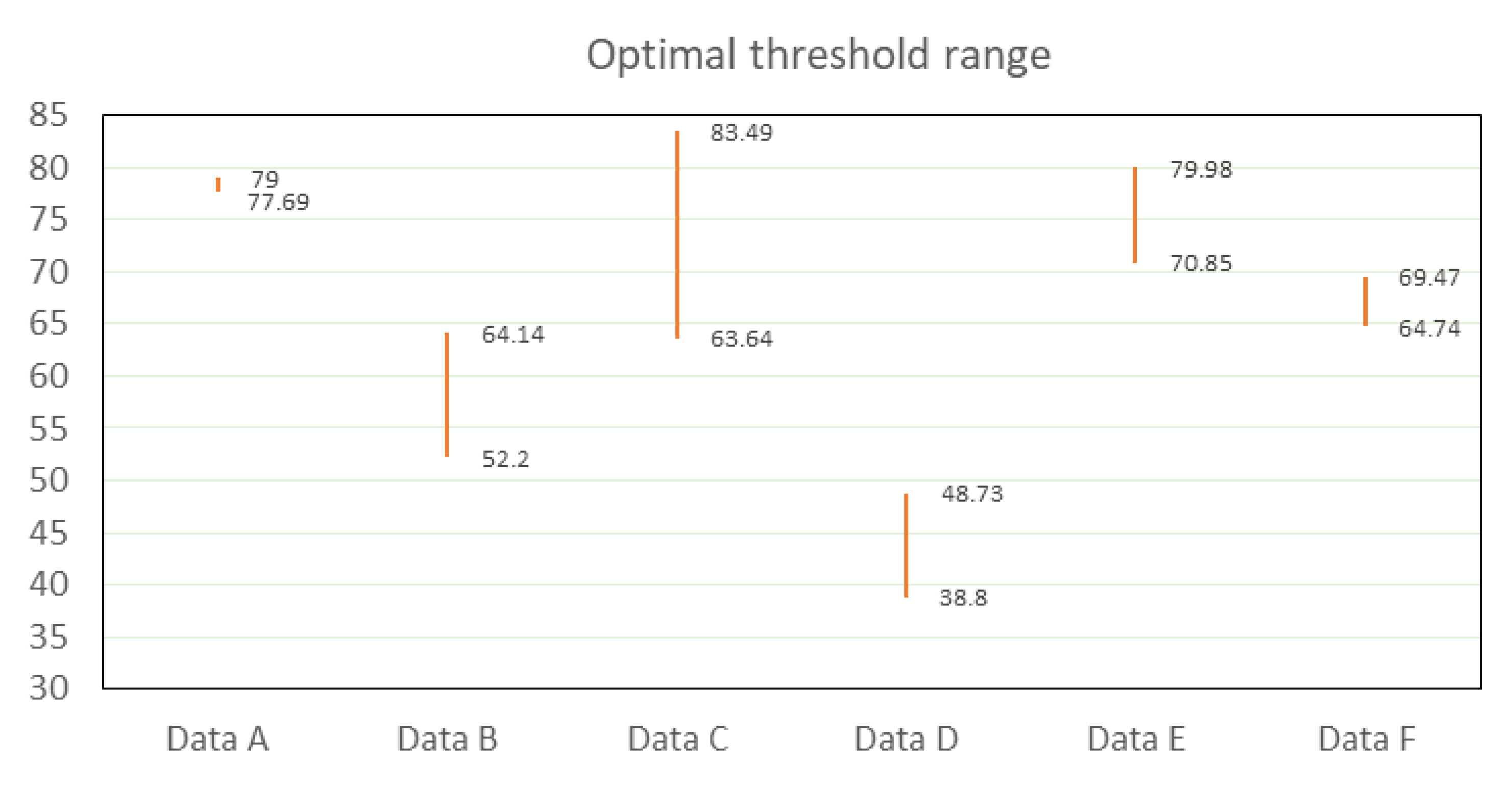
On the whole, it summarizes that the proposed method has the highest agreement with the reference image no matter what type of body of water, improving overall accuracy to over 99% as well as minimizing the error, and the three comprehensive indicators all show a significant improvement across the dataset. The proposed method in this paper set the optimal threshold to a range, but the threshold range was not absolute, only further limiting the weights of the graph cut model. In addition, according to Equation (14), the optimal threshold range [,] for the different data is shown in Figure 8.
In summary, the DTGC model has been proven to be a powerful and stable method for water binary classification, but there are still some factors affecting its accuracy.
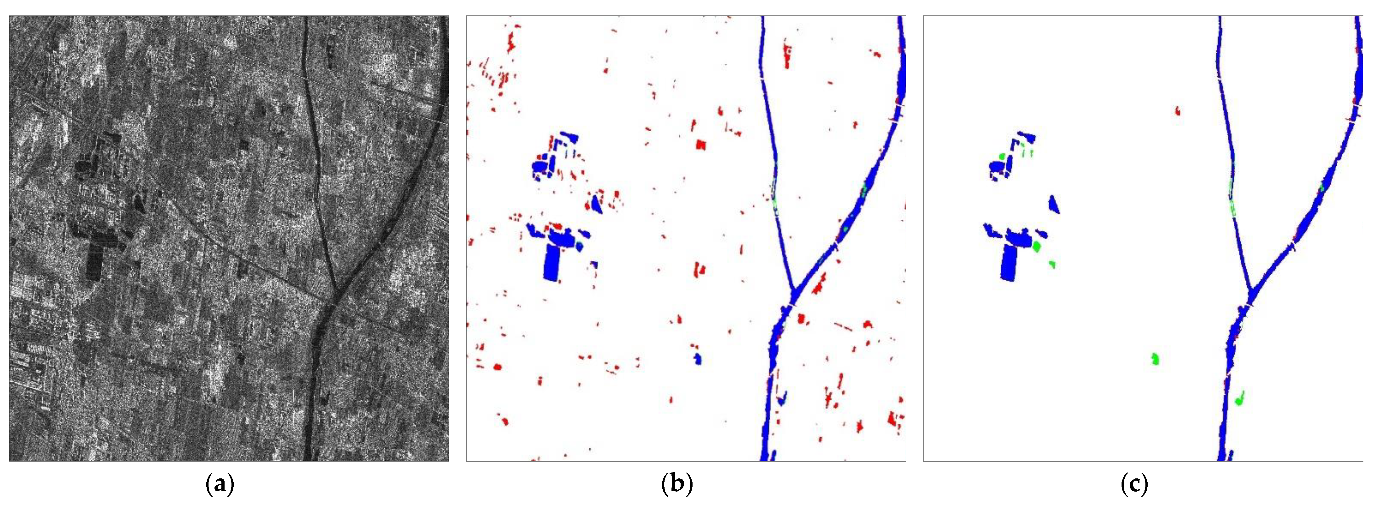
One is the noise interference problems. The accuracy of extracting is in general more susceptible to noise with similar properties of water, which creates a difficulty in distinguishing them with only a single SAR image; therefore, some of the reasons for a slight commission and omission error can be understood. Although postprocessing can further screen out the noise, it also brings about other problems. An example of this phenomenon is depicted in Figure 9. After the DTGC model is employed, despite a large number of false detections, water extraction is almost extracted completely. Then, postprocessing is carried out for the purpose of eliminating the false alarm errors as well as inevitably bringing about the missed detection, as shown in Figure 9c, which is also why most papers are more inclined to extract large, open-water bodies that are relatively concentrated and easy to filter.
The other is the boundary issue. The optimal threshold is limited to a custom range [,], which can detect almost 90% of the boundary, but by judging from the results, the ability to suppress boundary noise needs to be further improved. Furthermore, when the boundary of the water body is very close to the ships inside the target water, resampling may cause the loss of the boundary information, but this situation is still relatively rare.
Therefore, to present a more accurate and convincing picture of water extraction, it would be necessary to emphatically consider solving the above problems.
4.3. The Fitting Effect of Different Probability Distributions
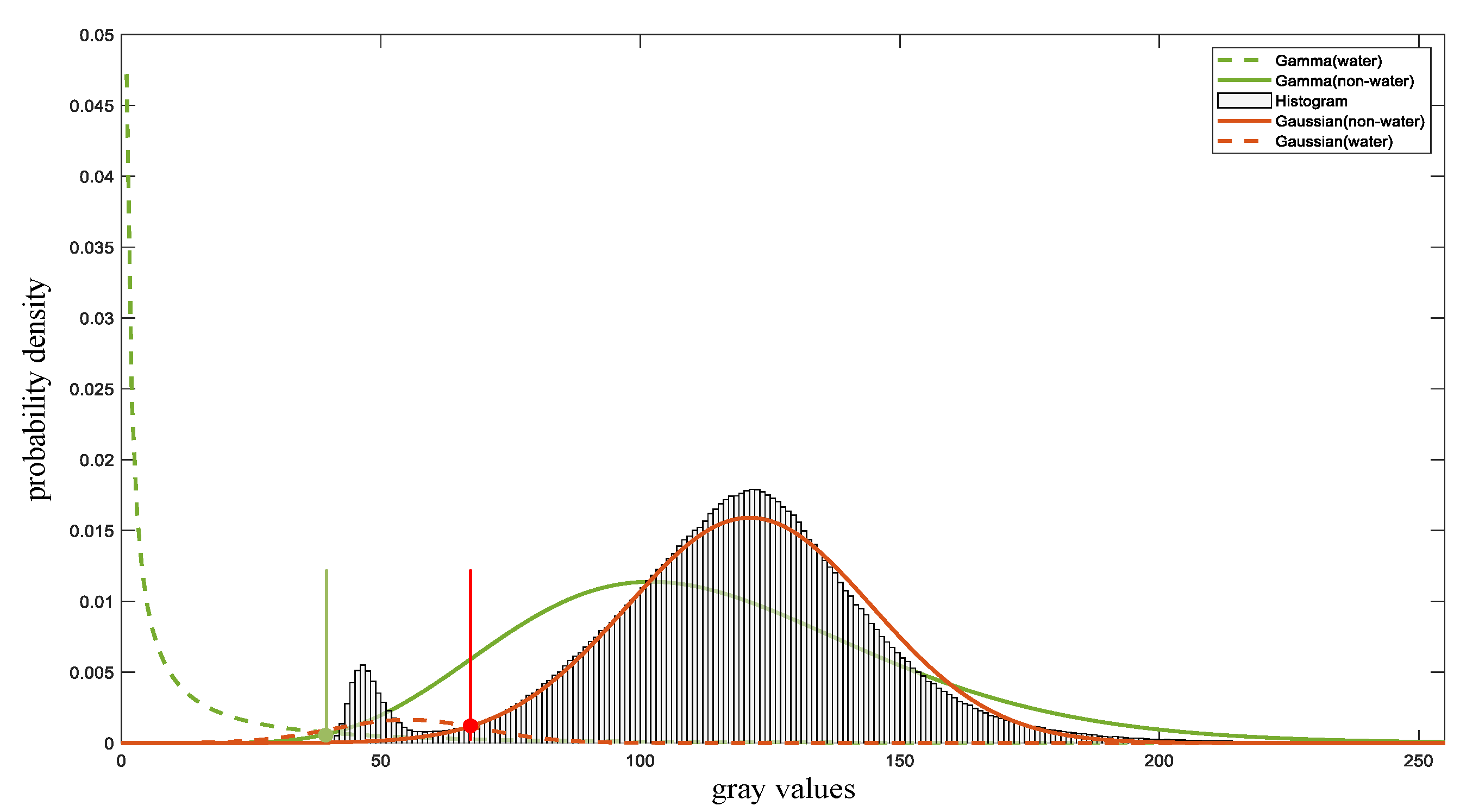
Many studies fit the SAR image intensity histogram with Gamma distribution [40] or Gaussian distribution [41]. Therefore, we chose Data F as an example to compare the above two distributions, and the results are shown in Figure 10 It can be clearly seen that the GMM intersection point (red) used in this paper is located near the trough, which is significantly better than the fitting effect of the Gamma distribution (green). Therefore, in this article, we did not hesitate to choose to use the Gaussian mixture model.
4.4. Algorithm Complexity
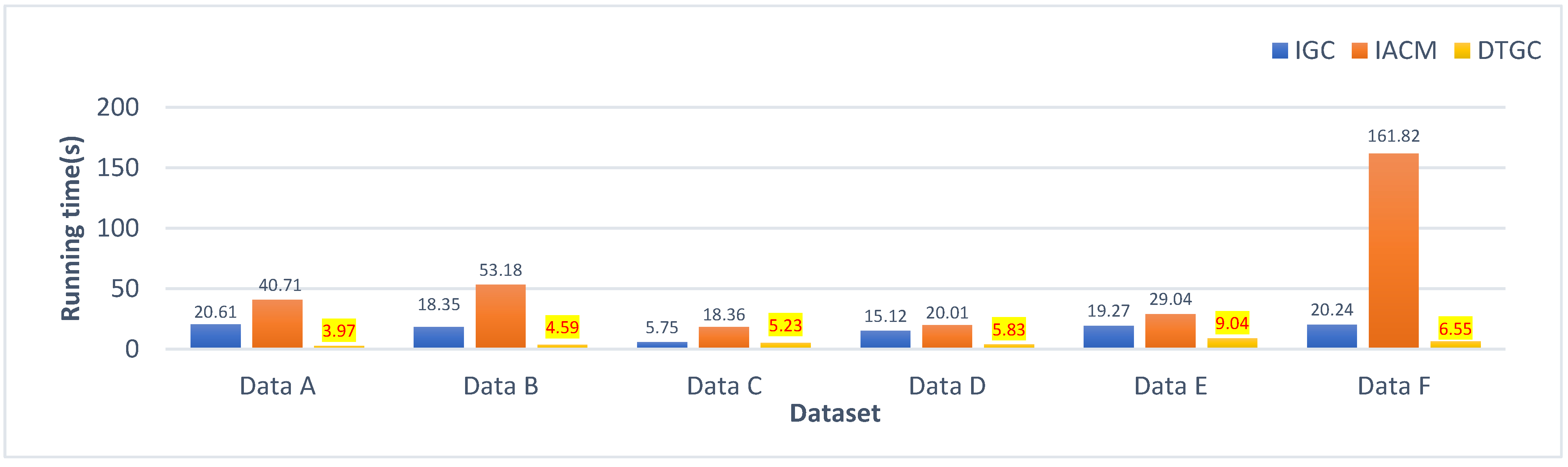
The running time is also a very important criterion to measure and analyze the computational efficiency of the three methods. Our experiment was done in the software MATLAB (2020) 64-bit operating system, and the hardware environment was AMD Ryzen 7 5800H 3.2 GHz and 16GB RAM. The runtimes for comparison are listed in Figure 11.
It is obvious that the proposed framework has the shortest running time and is far ahead of the comparison methods, indicating that the two measures of resampling and parallelism can effectively improve the running speed, whereas the repeated iterations of the EM algorithm in the IGC method and the ACM algorithm in the IACM method hinder their algorithm’s efficiency.
5. Conclusions
In the paper, we propose a novel and efficient algorithm for identifying water surface, not only notably improving the accuracy of classification in complex areas, but also expanding the scope of water body extraction. We first use the maximum to represent the texture feature of each scale in different directions and employ the Otsu algorithm to binarize the multiscale feature images generated by the Gabor filter, by taking advantage of more information during pixel-by-pixel classification. In addition, the initial segmentation image obtained by the voting strategy is explored for calculating the GMM parameters. This process effectively distinguishes the water from feature maps, which is capable of suppressing the coherent speckle noise, as well as greatly improving the fitting effect of Gaussian distributions of water and non-water. The experimental results demonstrate that the successful implementation of DTGC model has the following innovations:
- Locating the optimal threshold range by introducing the dual threshold. The dual-threshold is a good approach to determine threshold automatically. The DTGC model provides better results, pinpointing the water body location.
- Expanding the types of water bodies extracted from SAR images. The proposed method performs reliably better across open lakes, rivers, and complex areas than other traditional methods, making it a compelling classification tool.
- Achieving rapid and automatic extraction of various water types without requiring manual screening of thresholds and other specific prior knowledge.
The value of DTGC model combined with the multiscale Gabor filter is not only captured in solving a series of problems existing in traditional methods but also fully meets the demand of automatic, high accuracy, fast speed, and wide application. The experimental results also prove the universality and robustness of our method in processing the SAR images.
In the future work, we will continue to explore more models to improve the accuracy of water extraction from SAR image dataset under complex scenes, along with solving the problems mentioned in Section 4.2, as well as reducing the postprocessing steps.
Author Contributions
Conceptualization, L.B.; methodology, L.B.; software, L.B.; validation, L.B.; formal analysis, L.B.; investigation, L.B.; resources, L.B.; data curation, L.B.; writing—original draft preparation, L.B.; writing—review and editing, L.B. and X.L.; visualization, L.B.; supervision, L.B.; project administration, X.L. and J.Y.; funding acquisition, X.L and J.Y. All authors have read and agreed to the published version of the manuscript.
Funding
This research was supported by National Key Research and Development Program of China, grant number 2018YFC1505100 and the China Academy of Railway Sciences Fund, grant number 2019YJ028.
Institutional Review Board Statement
Not applicable.
Informed Consent Statement
Not applicable.
Data Availability Statement
The data that support the findings of this study are available from the corresponding author upon reasonable request.
Acknowledgments
The authors are thankful to the Copernicus Programme of the European Space Agency and Alaska Satellite Facility for freely providing the Sentinel-1 data, the remote sensing data sharing website (http://ids.ceode.ac.cn/) of the Institute of Remote Sensing and Digital Earth, Chinese Academy of Sciences, for freely providing the GF-3 data, and German Aerospace Agency for freely providing the TerraSAR-X data.
Conflicts of Interest
The authors declare no conflict of interest.
Appendix A
The appendix contains six SAR image data used in the paper, respectively, Data A–F, which are shown in Figure A1.
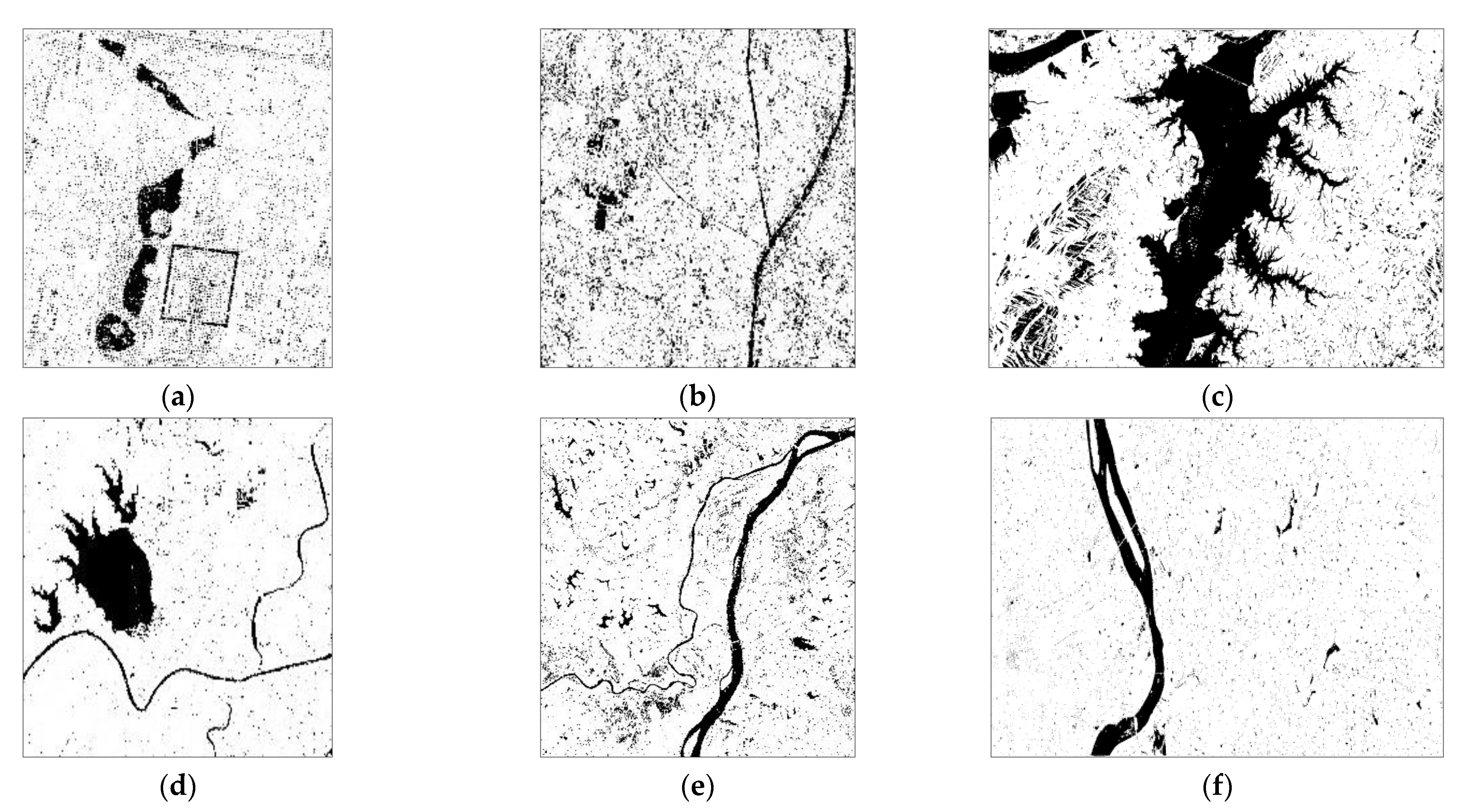
Figure A1.
The SAR images from Data A to Data F of the study area. (a): Data A, (b): Data B, (c): Data C, (d): Data D, (e):Data E, (f):Data F.
Figure A1.
The SAR images from Data A to Data F of the study area. (a): Data A, (b): Data B, (c): Data C, (d): Data D, (e):Data E, (f):Data F.


References
- Wang, Y.; Li, Z.; Zeng, C.; Xia, G.-S.; Shen, H. An Urban Water Extraction Method Combining Deep Learning and Google Earth Engine. IEEE J. Sel. Top. Appl. Earth Obs. Remote Sens. 2020, 13, 769–782. [Google Scholar] [CrossRef]
- Zhuang, Y.; Wang, P.; Yang, Y.; Shi, H.; Chen, H.; Bi, F. Harbor Water Area Extraction from Pan-Sharpened Remotely Sensed Images Based on the Definition Circle Model. IEEE Geosci. Remote Sens. Lett. 2017, 14, 1690–1694. [Google Scholar] [CrossRef]
- Yuan, J.; Lv, X.; Dou, F.; Yao, J. Change Analysis in Urban Areas Based on Statistical Features and Temporal Clustering Using TerraSAR-X Time-Series Images. Remote Sens. 2019, 11, 926. [Google Scholar] [CrossRef] [Green Version]
- Hoekstra, M.; Jiang, M.; Clausi, D.A.; Duguay, C. Lake Ice-Water Classification of RADARSAT-2 Images by Integrating IRGS Segmentation with Pixel-Based Random Forest Labeling. Remote Sens. 2020, 12, 1425. [Google Scholar] [CrossRef]
- Li, N.; Wang, R.; Deng, Y.; Chen, J.; Liu, Y.; Du, K.; Lu, P.; Zhang, Z.; Zhao, F. Waterline Mapping and Change Detection of Tangjiashan Dammed Lake After Wenchuan Earthquake from Multitemporal High-Resolution Airborne SAR Imagery. IEEE J. Sel. Top. Appl. Earth Obs. Remote Sens. 2014, 7, 3200–3209. [Google Scholar] [CrossRef]
- Bi, F.; Chen, J.; Wei, H.; Zhao, Y. A hierarchical method for accurate water region detection in SAR images. In Proceedings of the IET International Radar Conference 2015, Hangzhou, China, 14–16 October 2015; pp. 1–4. [Google Scholar]
- Zhou, Y.; Luo, J.; Shen, Z.; Hu, X.; Yang, H. Multiscale Water Body Extraction in Urban Environments from Satellite Images. IEEE J. Sel. Top. Appl. Earth Obs. Remote Sens. 2014, 7, 4301–4312. [Google Scholar] [CrossRef]
- Huang, X.; Xie, C.; Fang, X.; Zhang, L. Combining Pixel- and Object-Based Machine Learning for Identification of Water-Body Types from Urban High-Resolution Remote-Sensing Imagery. IEEE J. Sel. Top. Appl. Earth Obs. Remote Sens. 2015, 8, 2097–2110. [Google Scholar] [CrossRef]
- Guo, H.; He, G.; Jiang, W.; Yin, R.; Yan, L.; Leng, W. A Multi-Scale Water Extraction Convolutional Neural Network (MWEN) Method for GaoFen-1 Remote Sensing Images. ISPRS Int. J. Geoinf. 2020, 9, 189. [Google Scholar] [CrossRef] [Green Version]
- Katiyar, V.; Tamkuan, N.; Nagai, M. Near-Real-Time Flood Mapping Using Off-the-Shelf Models with SAR Imagery and Deep Learning. Remote Sens. 2021, 13, 2334. [Google Scholar] [CrossRef]
- Zhang, J.; Xing, M.; Sun, G. A Water Segmentation Algorithm for SAR Image Based on Dense Depthwise Separable Convolution. J. Radars 2019, 8, 400–412. [Google Scholar]
- Liu, Z.; Li, F.; Li, N.; Wang, R.; Zhang, H. A Novel Region-Merging Approach for Coastline Extraction From Sentinel-1A IW Mode SAR Imagery. IEEE Geosci. Remote Sens. Lett. 2016, 13, 324–328. [Google Scholar] [CrossRef]
- Du, Y.; Xu, J.; Liu, S. Water Self-extraction Algorithm From Remote Sensing Image Based on Improved Graph Cut. Comput. Eng. Design 2019, 40, 1413–1417. [Google Scholar]
- Leng, Y.; Liu, Z.; Zhang, H.; Wang, Y.; Li, N. Improved ACM Algorithm for Poyang Lake Monitoring. J. Electron. Inf. Technol. 2017, 39, 1064–1070. [Google Scholar]
- Ciecholewski, M. River channel segmentation in polarimetric SAR images: Watershed Transform Combined with Average Contrast Maximisation. Expert Syst. Appl. 2017, 82, 196–215. [Google Scholar] [CrossRef]
- Sghaier, M.O.; Foucher, S.; Lepage, R. River Extraction from High-Resolution SAR Images Combining a Structural Feature Set and Mathematical Morphology. IEEE J. Sel. Top. Appl. Earth Obs. Remote Sens. 2017, 10, 1025–1038. [Google Scholar] [CrossRef]
- Hu, S.; Qin, J.; Ren, J.; Zhao, H.; Ren, J.; Hong, H. Automatic Extraction of Water Inundation Areas Using Sentinel-1 Data for Large Plain Areas. Remote Sens. 2020, 12, 243. [Google Scholar] [CrossRef] [Green Version]
- Mao, C.; Wan, S. A Water/Land Segmentation Algorithm Based on an Improved Chan-Vese Model with Edge Constraints of Complex Wavelet Domain. Chin. J. Electron. 2015, 24, 361–365. [Google Scholar] [CrossRef]
- Zeng, L.; Schmitt, M.; Li, L.; Zhu, X.X. Analysing changes of the Poyang Lake water area using Sentinel-1 synthetic aperture radar imagery. Int. J. Remote Sens. 2017, 38, 7041–7069. [Google Scholar] [CrossRef] [Green Version]
- Ding, X.; Li, X. Monitoring of the water-area variations of Lake Dongting in China with ENVISAT ASAR images. Int. J. Appl. Earth Obs. Geoinf. 2011, 13, 894–901. [Google Scholar] [CrossRef]
- Xing, L.; Tang, X.; Wang, H.; Fan, W.; Wang, G. Monitoring monthly surface water dynamics of Dongting Lake using Sentinel-1 data at 10 m. PeerJ 2018, 6, e4992. [Google Scholar] [CrossRef] [PubMed]
- Niu, S.; Li, N.; Guo, Z.; Wang, R.; Guo, Y.; Wu, L.; Zhao, J. Robust boundary extraction of great lakes by blocking Active Contour Model using Chinese GF-3 SAR data: A case study of Danjiangkou reservoir, China. J. Eng. 2019, 2019, 6876–6879. [Google Scholar] [CrossRef]
- Ferrentino, E.; Nunziata, F.; Buono, A.; Urciuoli, A.; Migliaccio, M. Multi-polarization time-series of Sentinel-1 SAR imagery to analyze variations of reservoirs’ water-body. IEEE J. Sel. Top. Appl. Earth Obs. Remote Sens. 2020, 13, 840–846. [Google Scholar] [CrossRef]
- Li, Y.; Yang, Y.; Zhao, Q. Urban Riverway Extraction from High-Resolution SAR Image Based on Blocking Segmentation and Discontinuity Connection. Remote Sens. 2020, 12, 4014. [Google Scholar] [CrossRef]
- Mason, D.C.; Speck, R.; Devereux, B.; Schumann, G.J.P.; Neal, J.C.; Bates, P.D. Flood Detection in Urban Areas Using TerraSAR-X. IEEE Trans. Geosci. Remote Sens. 2010, 48, 882–894. [Google Scholar] [CrossRef] [Green Version]
- Zeng, C.; Wang, J.; Huang, X.; Bird, S.; Luce, J.J. Urban water body detection from the combination of high-resolution optical and SAR images. In Proceedings of the 2015 Joint Urban Remote Sensing Event (JURSE), Lausanne, Switzerland, 30 March–1 April 2015. [Google Scholar]
- Feyisa, G.L.; Meilby, H.; Fensholt, R.; Proud, S.R. Automated Water Extraction Index: A new technique for surface water mapping using Landsat imagery. Remote Sens. 2014, 140, 23–35. [Google Scholar] [CrossRef]
- Liang, J.; Liu, D. A local thresholding approach to flood water delineation using Sentinel-1 SAR imagery. ISPRS J. Photogramm. Remote Sens. 2020, 159, 53–62. [Google Scholar] [CrossRef]
- Sun, Z.; Zhang, Z.; Chen, Y.; Liu, S.; Song, Y. Frost Filtering Algorithm of SAR Images with Adaptive Windowing and Adaptive Tuning Factor. IEEE Geosci. Remote Sens. Lett. 2020, 17, 1097–1101. [Google Scholar] [CrossRef]
- Greig, D.M.; Porteous, B.T.; Seheult, A.H. Exact Maximum A Posteriori Estimation for Binary Images. J. R. Stat. Soc. 1989, 51, 271–279. [Google Scholar] [CrossRef]
- Meng, Q.; Wen, X.; Yuan, L.; Xu, H. Factorization-Based Active Contour for Water-Land SAR Image Segmentation via the Fusion of Features. IEEE Access 2019, 7, 40347–40358. [Google Scholar] [CrossRef]
- Otsu, N. A Threshold Selection Method from Gray-Level Histograms. IEEE Trans. Syst. Man Cybern. 1979, 9, 62–66. [Google Scholar] [CrossRef] [Green Version]
- Deng, Y.; Zhang, H.; Wang, C.; Liu, M. Object-oriented water extraction of PolSAR image based on target decomposition. In Proceedings of the 2015 IEEE 5th Asia-Pacific Conference on Synthetic Aperture Radar (APSAR), Singapore, 1–4 September 2015; pp. 596–601. [Google Scholar]
- Dempster, A.P. Maximum likelihood from incomplete data via the EM algorithm. J. R. Stat. Soc. 1977, 39, 1–38. [Google Scholar]
- Zhao, B.; Zhong, Y.; Ma, A.; Zhang, L. A Spatial Gaussian Mixture Model for Optical Remote Sensing Image Clustering. IEEE J. Sel. Top. Appl. Earth Obs. Remote Sens. 2016, 9, 5748–5759. [Google Scholar] [CrossRef]
- Xiao, P.; Yuan, M.; Zhang, X.; Feng, X.; Guo, Y. Cosegmentation for Object-Based Building Change Detection from High-Resolution Remotely Sensed Images. IEEE Trans. Geosci. Remote Sens. 2017, 55, 1587–1603. [Google Scholar] [CrossRef]
- Zhang, K.; Fu, X.; Lv, X.; Yuan, J. Unsupervised Multitemporal Building Change Detection Framework Based on Cosegmentation Using Time-Series SAR. Remote Sens. 2021, 13, 471. [Google Scholar] [CrossRef]
- Boykov, Y.; Kolmogorov, V. An experimental comparison of min-cut/max- flow algorithms for energy minimization in vision. IEEE Trans. Pattern Anal. Mach. Intell. 2004, 26, 1124–1137. [Google Scholar] [CrossRef] [Green Version]
- Chen, P.; Cai, X.; Zhao, D.; Liang, R.; Intelligence, M. Side scan sonar image speckle noise reduction based on adaptive BM3D. Opto-Electron. Eng. 2020, 47, 71–80. [Google Scholar]
- Giustarini, L.; Hostache, R.; Kavetski, D.; Chini, M.; Corato, G.; Schlaffer, S.; Matgen, P. Probabilistic Flood Mapping Using Synthetic Aperture Radar Data. IEEE Trans. Geosci. Remote Sens. 2016, 54, 6958–6969. [Google Scholar] [CrossRef]
- Giustarini, L.; Hostache, R.; Matgen, P.; Schumann, G.J.P.; Bates, P.D.; Mason, D.C. A Change Detection Approach to Flood Mapping in Urban Areas Using TerraSAR-X. IEEE Trans. Geosci. Remote Sens. 2013, 51, 2417–2430. [Google Scholar] [CrossRef] [Green Version]
Figure 1.
The overview of this study. The parameters and are the number of scales and directions of Gabor filter. The parameter is a feature threshold of voting strategy.
Figure 1.
The overview of this study. The parameters and are the number of scales and directions of Gabor filter. The parameter is a feature threshold of voting strategy.

Figure 2.
The fitting effect of GMM for the SAR image. (a) The histogram of gray values. (b) The fitted GMM distribution curves of water () and non-water ().
Figure 2.
The fitting effect of GMM for the SAR image. (a) The histogram of gray values. (b) The fitted GMM distribution curves of water () and non-water ().

Figure 3.
An example of graph cut segmentation for a simple 3 × 3 image (adapted from [36]).
Figure 3.
An example of graph cut segmentation for a simple 3 × 3 image (adapted from [36]).

Figure 4.
The optimal feature maps of Data A. (a–e) are maps of a scale 1–5, respectively.

Figure 5.
(a–f) are the initial segmentation results from Data A to Data F. The black and white pixels indicate water and non-water, respectively.
Figure 5.
(a–f) are the initial segmentation results from Data A to Data F. The black and white pixels indicate water and non-water, respectively.

Figure 6.
The water segmentation results by using different methods on dataset. (a1–f1) are the original images, (a2–f2) are the manually labeled ground truth. (a3–f3), (a4–f4), and (a5–f5) are the extraction outcomes of the proposed method, IGC method in [13], and IACM method in [14]. The highlighted colors in the results represent water (blue), omission error (green), and commission error (red).


Figure 7.
The above classification results for the zoomed-in region ①–④ of Data C–F. (a): SAR image, (b): the ground truth, (c): DTGC method, (d): IGC method, and (e): IACM method. The highlighted colors in results represent water (blue), omission error (green), and commission error (red).
Figure 7.
The above classification results for the zoomed-in region ①–④ of Data C–F. (a): SAR image, (b): the ground truth, (c): DTGC method, (d): IGC method, and (e): IACM method. The highlighted colors in results represent water (blue), omission error (green), and commission error (red).

Figure 8.
The optimal threshold range of Data A–F.

Figure 9.
The results classified without and with postprocessing in Data B. (a): SAR image, (b): result without postprocessing, and (c): result with postprocessing.
Figure 9.
The results classified without and with postprocessing in Data B. (a): SAR image, (b): result without postprocessing, and (c): result with postprocessing.

Figure 10.
The comparison of Gamma distribution (green) and Gaussian distribution (red) for fitting the intensity histogram of Data F.
Figure 10.
The comparison of Gamma distribution (green) and Gaussian distribution (red) for fitting the intensity histogram of Data F.

Figure 11.
Runtimes of the various methods using dataset.


Table 1.
Weight Setting.
| Edge Type | Weight | Condition |
|---|---|---|
| 0 | ||
| 0 |
Table 2.
List of SAR dataset used in this work.
| Scheme | Satellite | Size | Location | Type | Polarization | Date |
|---|---|---|---|---|---|---|
| Data A | TerraSAR-X | 2404 × 2638 | Chaoyang District, Beijing | Urban water | HH | 9 May 2013 |
| Data B | GF-3 | 2444 × 2444 | Fangshan District, Beijing | Urban water | HH | 28 July 2017 |
| Data C | Sentinal-1 | 4669 × 3032 | Poyang Lake, Jiangxi | Lakes | VH | 8 July 2020 |
| Data D | Sentinal-1 | 2965 × 1735 | East Lake, Hunan | Lakes and rivers | VH | 25 September 2016 |
| Data E | Sentinal-1 | 2765 × 3007 | Poyang Lake, Jiangxi | Small tributary | VH | 8 July 2020 |
| Data F | TerraSAR-X | 6626 × 5273 | Xiangjiang, Hunan | Rivers | HH | 24 July 2020 |
Table 3.
Parameter setting of three methods.
| Parameter | Data A | Data B | Data C | Data D | Data E | Data F |
|---|---|---|---|---|---|---|
| 0.3 | 0.45 | 0.35 | 0.75 | 0.8 | 0.5 | |
| 0.2 | 0.25 | 0.2 | 0.45 | 0.2 | 0.2 | |
| 0.8 | 0.25 | 0.9 | 0.2 | 0.2 | 0.2 | |
| 10 | 10 | 5 | 10 | 20 | 20 |
Table 4.
Parameter setting of three methods.
| Image | Data A | Data B | Data C | Data D | Data E | Data F |
|---|---|---|---|---|---|---|
| Original | 12.71 | 9.55 | 5.66 | 10.40 | 11.94 | 17.60 |
| Denoised | 3.52 | 3.26 | 4.36 | 8.57 | 9.80 | 5.02 |
Table 5.
Water body extraction accuracy of the various methods.
| Test data | Method | OA(%) | Pre(%) | Rec(%) | Kappa | F1-score | IoU |
|---|---|---|---|---|---|---|---|
| Data A | IGC | 90.91 | 72.48 | 99.31 | 0.826 | 0.838 | 0.721 |
| IACM | 95.27 | 55.69 | 99.09 | 0.689 | 0.713 | 0.554 | |
| DTGC | 99.70 | 96.26 | 98.82 | 0.972 | 0.975 | 0.952 | |
| Data B | IGC | 18.12 | 3.18 | 99.96 | 0.010 | 0.062 | 0.032 |
| IACM | 65.59 | 4.35 | 56.08 | 0.032 | 0.081 | 0.042 | |
| DTGC | 99.50 | 90.13 | 92.46 | 0.906 | 0.908 | 0.832 | |
| Data C | IGC | 99.03 | 98.34 | 97.08 | 0.971 | 0.977 | 0.955 |
| IACM | 98.92 | 95.99 | 99.09 | 0.968 | 0.975 | 0.952 | |
| DTGC | 99.16 | 96.91 | 99.22 | 0.975 | 0.981 | 0.962 | |
| Data D | IGC | 98.77 | 88.51 | 99.69 | 0.931 | 0.938 | 0.883 |
| IACM | 98.94 | 90.00 | 99.73 | 0.940 | 0.946 | 0.900 | |
| DTGC | 99.46 | 96.61 | 98.13 | 0.970 | 0.972 | 0.946 | |
| Data E | IGC | 99.04 | 87.62 | 96.28 | 0.912 | 0.917 | 0.847 |
| IACM | 92.16 | 41.13 | 97.40 | 0.547 | 0.580 | 0.408 | |
| DTGC | 99.24 | 90.64 | 96.32 | 0.929 | 0.934 | 0.876 | |
| Data F | IGC | 99.66 | 92.13 | 99.45 | 0.955 | 0.957 | 0.917 |
| IACM | 99.63 | 91.28 | 99.53 | 0.950 | 0.952 | 0.909 | |
| DTGC | 99.88 | 99.13 | 97.72 | 0.983 | 0.984 | 0.969 |
The bolded data represents the highest data, which mainly further emphasizes the superiority of our proposed algorithm.
Publisher’s Note: MDPI stays neutral with regard to jurisdictional claims in published maps and institutional affiliations. |
© 2021 by the authors. Licensee MDPI, Basel, Switzerland. This article is an open access article distributed under the terms and conditions of the Creative Commons Attribution (CC BY) license (https://creativecommons.org/licenses/by/4.0/).
Share and Cite
MDPI and ACS Style
Bao, L.; Lv, X.; Yao, J. Water Extraction in SAR Images Using Features Analysis and Dual-Threshold Graph Cut Model. Remote Sens. 2021, 13, 3465. https://doi.org/10.3390/rs13173465
AMA Style
Bao L, Lv X, Yao J. Water Extraction in SAR Images Using Features Analysis and Dual-Threshold Graph Cut Model. Remote Sensing. 2021; 13(17):3465. https://doi.org/10.3390/rs13173465
Chicago/Turabian StyleBao, Linan, Xiaolei Lv, and Jingchuan Yao. 2021. "Water Extraction in SAR Images Using Features Analysis and Dual-Threshold Graph Cut Model" Remote Sensing 13, no. 17: 3465. https://doi.org/10.3390/rs13173465
Note that from the first issue of 2016, this journal uses article numbers instead of page numbers. See further details here.