Spatial-Aware Network for Hyperspectral Image Classification

Abstract

Deep learning is now receiving widespread attention in hyperspectral image (HSI) classification. However, due to the imbalance between a huge number of weights and limited training samples, many problems and difficulties have arisen from the use of deep learning methods in HSI classification. To handle this issue, an efficient deep learning-based HSI classification method, namely, spatial-aware network (SANet) has been proposed in this paper. The main idea of SANet is to exploit discriminative spectral-spatial features by incorporating prior domain knowledge into the deep architecture, where edge-preserving side window filters are used as the convolution kernels. Thus, SANet has a small number of parameters to optimize. This makes it fit for small sample sizes. Furthermore, SANet is able not only to aware local spatial structures using side window filtering framework, but also to learn discriminative features making use of the hierarchical architecture and limited label information. The experimental results on four widely used HSI data sets demonstrate that our proposed SANet significantly outperforms many state-of-the-art approaches when only a small number of training samples are available.

1. Introduction

Hyperspectral images (HSIs) usually contain abundant spectral information [1,2,3,4]. Such rich spectral information makes it possible to distinguish subtle spectral differences of different materials. Consequently, HSI classification has been widely used in a variety of applications, including environmental management [5], agriculture [6], and surveillance [7]. Over the past few decades, a large number of methods have been proposed to predict the class label of each pixel in HSI. However, it is still a challenging issue in HSI [4,8,9,10,11,12,13,14,15]. One of the most challenging issues is the limited available training samples. The reason for this is that it is difficult and time consuming to collect a large number of training samples [4,16].

The early research on HSI classification mainly focuses on exploring spectral features directly from spectrum, such as methods based on dimensionality reduction [17,18] and band selection [19]. However, due to the spatial variability and spectral heterogeneity of land covers, spectral-only methods usually fail to provide better performance. It is well known that neighborhood pixels in HSI are highly correlated [20]. As a result, a lot of efforts have been dedicated to integrate the spatial and spectral information for HSI classification [21]. In the past few years, a wide variety of spectral-spatial methods have been developed [20,22,23]. For example, extended morphological profiles (EMPs) is proposed to integrate spectral and spatial information in HSI [24]. In addition, a discriminative low-rank Gabor filtering method is also used to extract spatial-spectral features of HSI [25]. In [26], edge-preserving filtering (EPF) is used for obtaining spectral-spatial features of HSI for the first time. Random fields technology has also been widely used for incorporating spatial information into HSI classification, such as Markov random field (MRF) [27] and conditional random field (CRF) [28]. Moreover, sparsity has been used as a constraint to extract spectral-spatial features in different ways [29,30,31,32,33,34,35,36,37]. Recently, segmentation-based strategy is used to produce more spatially homogeneous classification maps [38,39,40,41]. Zehtabian et al. propose an approach for the development of automatic object-based techniques used for HSI classification [41]. Zheng et al. design a spectral-spatial HSI classificaion method that is based on superpixel segmentation and distance-weighted linear regression classifier to tackle the small labeled training sample size problem [41]. Although these methods can extract spectral-spatial features for HSI classification, low-level features are more sensitive to local changes occurred in HSI, especially in the case of small training samples [42].

The past few years have witnessed a surge of interest in deep learning [2,43]. Motivated by its success in natural image processing, a growing number of deep learning methods are designed for HSI classification [4,44,45]. In the early stages, stacked autoencoders (SAEs) and deep belief networks (DBNs) have been used for HSI classification in [46,47], respectively. This research attempts to intuitively feed the vector-based input into unsupervised deep learning models. However, this strategy suffers from spatial information loss. In order to address this issue, convolutional neural networks (CNNs) are used to learn effective spectral-spatial features residing in HSI [4]. For instance, Cao et al. adopted the CNN to extract deep spatial features [48]. In [49], 3D CNN is also adopted to extract spectral-spatial features. Furthermore, a 3D generative adversarial network (3D-GAN) is also applied in HSI classification [50], where adversarial samples are used as training samples. Although remarkable progress has been made in deep learning-based HSI classification, there still exist some important issues should be dealt with [4,12]. One of the most important issues is the imbalance between lots of weights and a small number of available samples [4,12,51]. That is, the training samples are usually very limited while deep learning models usually require a large number of samples to train [4,11,21]. Although some methods have been designed to deal with this problem, it is still an open problem. For example, RPNet has been proposed in [52], but the discrimination ability of random patches are not guaranteed.

As it is well known, one of the essential theories of deep learning is to learn effective features using a hierarchical architecture [11,21]. Furthermore, existing research shows that incorporating prior domain knowledge into deep learning models can promote their performance and reduce sample complexity [53]. Consequently, designing a deep learning method by incorporating the prior knowledge of HSI is a feasible way to promote the classification performance. In HSI classification, structure-preserving is one kinds of well known prior information, which has been widely used to extract spatial information by using filtering technology [26,54,55,56]. However, traditional smoothing filters, whose centers are aligned with the pixels being processed, usually lead to edge blurring and loss of spatial information [57]. Recently, side window filtering (SWF), which aligns the window’s side or corner with the pixel being processed, is proposed to handle an edge blurring problem in traditional filters [57]. As a result, SWF may outperform traditional smoothing filters in HSI analysis and classification.

Based on the discussion above, this paper will present a deep learning model called a spatial-aware network (SANet) for HSI classification. The proposed method can learn spectral-spatial features with a small amount of training samples. In summary, the major contributions of proposed SANet are twofold.

• This paper incorporates, for the first time in the literature, a side window filtering framework into deep architecture for HSI classification. We utilize SWF to effectively discover the spatial structure information in HSIs.
• This paper proposes an effective deep learning method. There are only a very small number of parameters that need to be determined. Thus, the proposed method can efficiently learn the spectral-spatial features by using a small number of training samples.

This paper is organized in the following manner: Section 2 gives a detailed description of the SANet for HSI classification. Section 3 validates the effectiveness of the proposed SANet on four typical data sets. The comprehensive comparison with several state-of-the-art methods is also presented. Finally, conclusions are drawn in Section 4.

2. Methodology

2.1. Spatial-Aware Network for Feature Learning

Figure 1 details the overall flowchart of our proposed SANet, where only six hidden layers are shown for clarity. In contrast to the traditional deep learning methods, which adopt an end-to-end approach to learn, there is no back propagation during the implementation of SANet. Instead, by using the predefined convolutional filters (side window filters), SANet can extract deep features efficiently. By convolving side window filters and integrating them into a deep hierarchical architecture to form SANet, we not only retain the characteristics of side window filtering but also give play to the powerful feature learning ability of deep learning. As shown in Figure 1, SANet has a hierarchical architecture, which includes F layer, P layer, and R layer, where the F layer combines their inputs with different filters to extract spatial features, P layer outputs the structure-preserving responses, and R layer processes their inputs by a supervised dimension reduction method, thereby increasing discriminability and reducing redundancy. These three layers can form one spectral-spatial feature learning unit. The detailed descriptions are as follows.

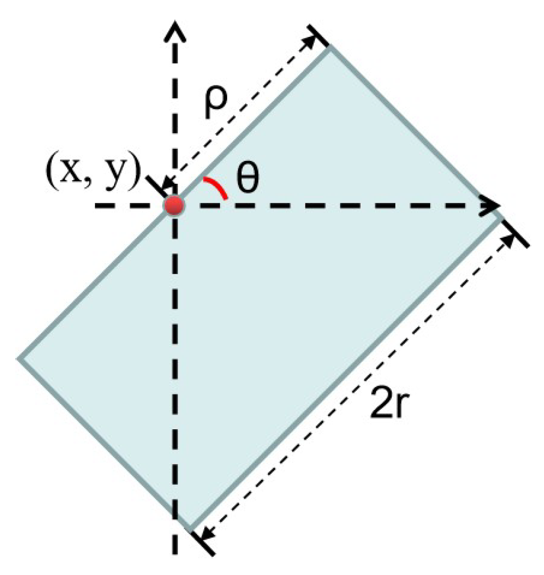
$F_1$Layer: Let $\mathbf{X}\in R^{m\times n\times b}$ be the original HSI, where m, n, b are the row number, column number, and band number, respectively. Let ${\mathbf{X}}_i$ represent the ith band of the input HSI, and ${\mathbf{X}}_i(x,y)$ is the reflectance value at the position $(x,y)$. ${\mathbf{X}}_i$ can be filtered using different side windows with different radius. Figure 2 shows the definition of continuous side window, where $(x,y)$ is the position of the pixel being processed, $\theta$ denotes the window orientation, r represents the radius of the window (can be predefined by users), and $\rho \in [0,r]$. By changing $\theta$ and $\rho$, different side windows can be obtained, where the pixel being processed should be on the side or corner of the window.

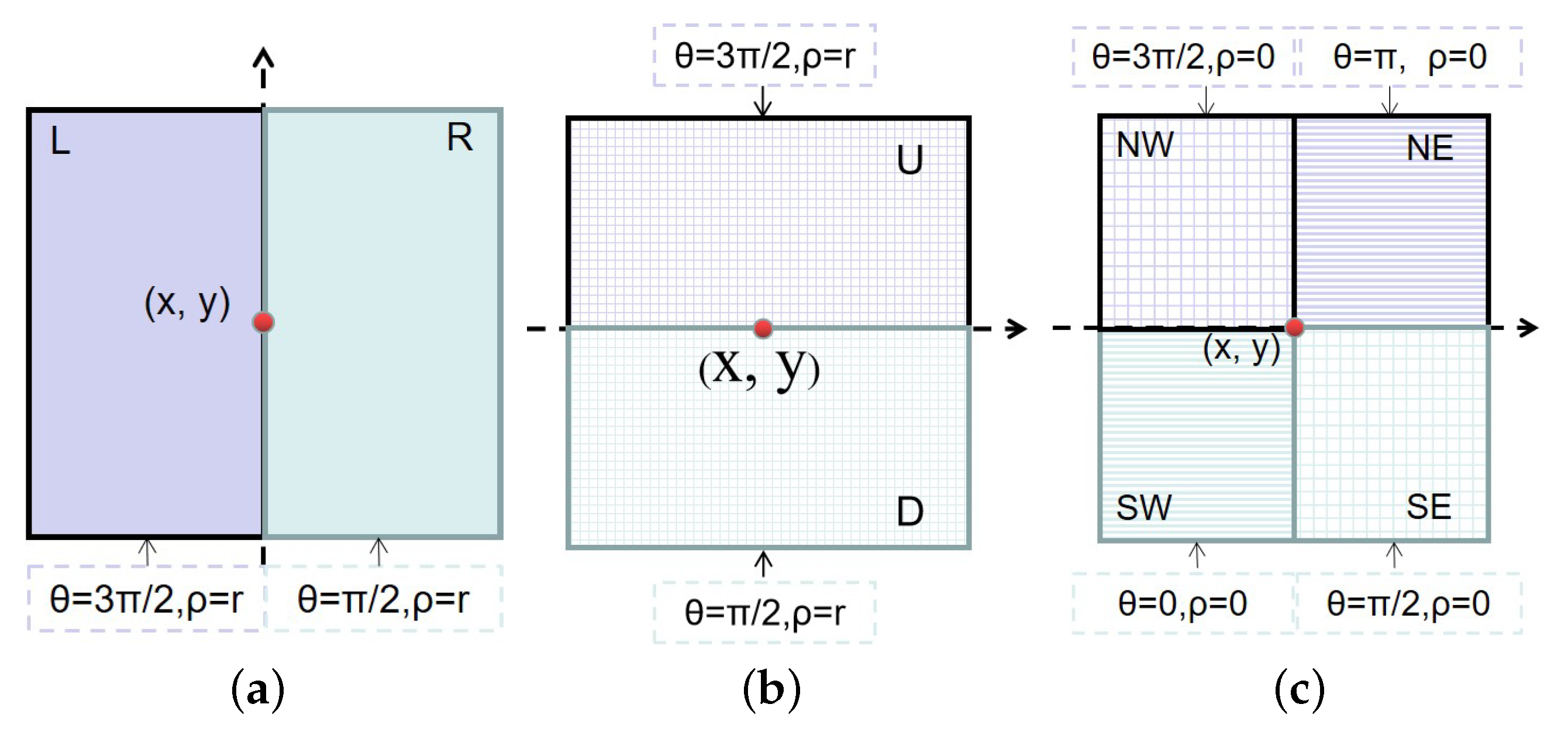
In practice, there are only a limited quantity of side windows that can be used, where Figure 3 shows eight side windows. These side windows correspond to $\theta =k\times \frac{\pi }{2}(k\in [0,3])$ and $\rho =\{0,r\}$. Letting $\rho =r$, we can obtain four side windows, which are shown in Figure 3a,b. If we set $\rho =0$, we can get another four side windows, which can be found in Figure 3c. In this paper, eight side windows shown in Figure 3 are used for exploring the spatial information in HSI. Note that we can design more side windows with different sizes, shapes, and orientations by changing r, $\theta$, and $\rho$.

Note that the side window technique can be embedded into a wide variety of filters, such as Gaussian filter, median filter, bilateral filter, and guided filter. In this paper, box filter is used for simplicity. Then, the output is given by

$${\mathbf{X}}_i^{F_1,\theta ,\rho ,r_j}(x,y)=\widehat{F}({\mathbf{X}}_i(x,y),\theta ,\rho ,r_j),$$

(1)

where $\widehat{F}$ stands for filtering operation, $r_j$ is the radius of the window, and $j=1,2,\cdots \widehat{r}$ ($\widehat{r}$ is the total number of the radius). Here, different $r_j$ corresponds to different scales. On each scale, eight side windows ($L,R,U,D,SW,SE,NE,NW$ denoted in Figure 3) have been used in this paper. Thus, we can obtain eight feature maps on each scale. Note that only one scale is used in Figure 1 for illustration purposes only. The filtering results on the i-th band are denoted by ${\mathbf{X}}_i^{F_1}$. Figure 4 shows the multiscale filtering on the ith band. We can carry out this operation on all of the bands. Thus, the total number of the feature maps is $N=\widehat{r}\times b\times 8$. Finally, the output of this layer is denoted by ${\mathbf{X}}^{F_1}\in R^{m\times n\times N}$.

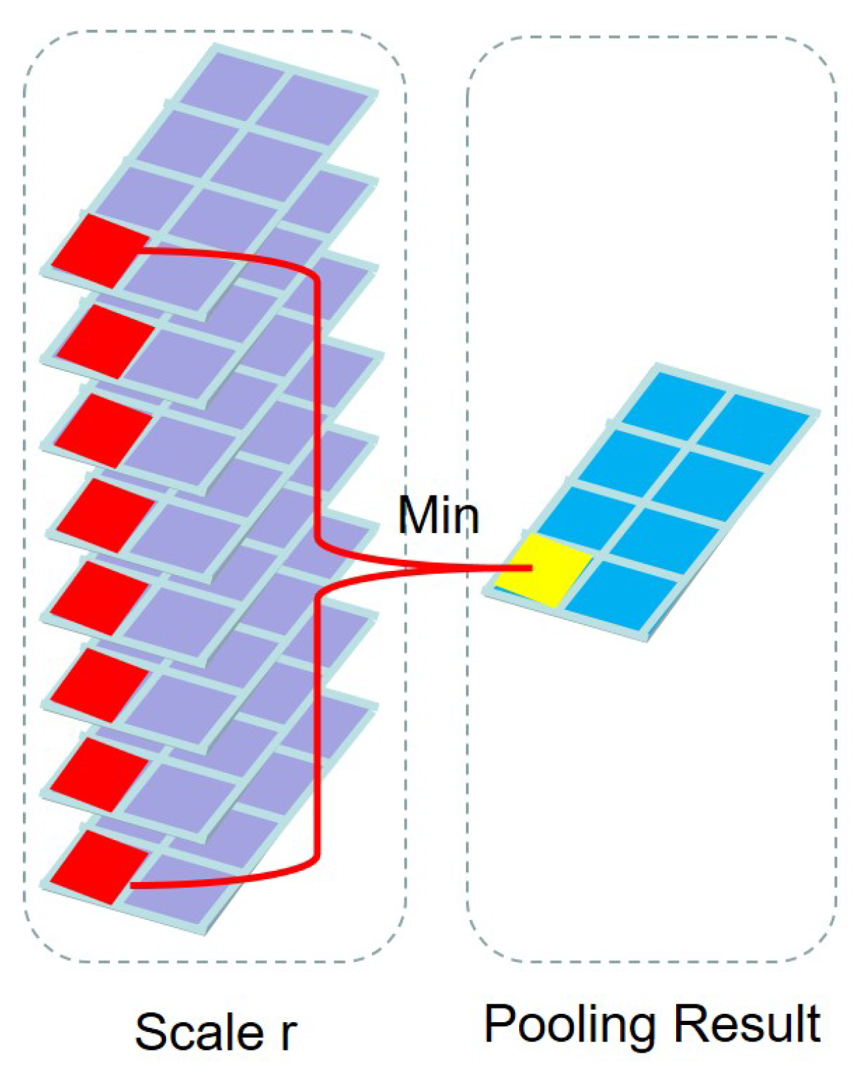
$P_1$Layer: In this layer, the MIN pooling is operated over different maps belonging to the same scale. That is, we keep only the minimum output over eight feature maps belonging to the same scale at each position. That is,

$${\mathbf{P}}_i^{P_1,r_j}(x,y)=\underset{\theta =k\times \frac{\pi }{2}(k\in [0,3]),\rho \in \{0,r_j\}}{min}{\mathbf{X}}_i^{F_1,\theta ,\rho ,r_j}(x,y),$$

(2)

where ${\mathbf{P}}_i^{P_1,r_j}(x,y)$ is the element of ${\mathbf{P}}_i^{P1,r_j}$ in the xth row and yth column. Hence, one scale band is formed by eight feature maps with the same scale in the output of F1 layer (see Figure 5). Finally, we can obtain the feature map ${\mathbf{P}}^{P_1}\in R^{m\times n\times b\widehat{r}}$.

$R_1$Layer: In this layer, feature fusion is carried out to reduce the redundant information residing in high-dimensional ${\mathbf{P}}^{P_1}$. Thus, this layer is also called feature fusion layer. This feature fusion operation can not only reduce redundancy but also speeding up the following feature learning. In theory, any feature fusion methods can be used in this layer. For simplicity, linear discriminant analysis (LDA) is adopted in this paper. It can not only reduce the dimension of the data but also able to increase the discriminability of the learned spectral-spatial features. Therefore, the stacked feature maps in ${\mathbf{P}}^{P_1}$ are fused together as follows:

$${\mathbf{Y}}^{R_1}(x,y)={\left({\mathbf{P}}^{P_1}(x,y)\right)}^T\mathbf{A},$$

(3)

where $\mathbf{A}$ is the LDA projection matrix learned from the training samples and consists of S projection directions. Finally, the output of this layer can be denoted by ${\mathbf{Y}}^{R_1}\in R^{m\times n\times S}$.

Feature Learning in Deep Layers: Let ${\mathbf{Y}}^{R_{h-1}}$ denote the output of the $R_{h-1}$ layer. For purpose of learning spectral-spatial features in higher layers, we can take ${\mathbf{Y}}^{R_{h-1}}$ as the input data and perform the same operations with in $F_1$ layer, $P_1$ layer and $R_1$ layer. In this way, we can obtain spectral-spatial features from different layers as $\{{\mathbf{Y}}^{R_1},{\mathbf{Y}}^{R_2},\cdots ,{\mathbf{Y}}^{R_h}\}$. In this paper, $F_i$, $P_i$, and $R_i$, which are carried out successively, form the ith spectral-spatial feature learning unit. The number of the feature learning units represents the depth of the proposed deep model. Consequently, we can learn deep spectral-spatial features with increasing depth.

2.2. Classification Layer

In this layer, the learned spectral-spatial features are fed into classifiers. Previous studies have shown that different layers of deep model can extract different levels of spectral-spatial features [58]. Low-level features always contain more detailed information, and high-level features are more invariant. All of these features are very important for HSI classification. It is reasonable to use both high-level and low-level features for robust HSI classification. Based on this observation, $\{{\mathbf{Y}}^{R_1},{\mathbf{Y}}^{R_2},\cdots ,{\mathbf{Y}}^{R_L}\}$ are concatenated for HSI classification, where L is the number of the spectral-spatial feature learning units. Finally, these concatenated spectral-spatial features are fed into SVM for classification.

The pseudocode of the SANet is detailed in Algorithm 1, where ${\mathbf{T}}_r$ consists of indexes and labels of the training samples. For the sake of convenience, the original input HSI is denoted by ${\mathbf{Y}}^{R_0}$. As can be seen, the proposed SANet is easy to implement.

Algorithm 1 SANet

Require: $\mathbf{X}\in R^{m\times n\times b}$, $T_r=[{\mathbf{I}}_x,{\mathbf{I}}_y,\mathbf{L}]$. Ensure: Predicted Labels. 1: ${\mathbf{Y}}^{R_0}=\mathbf{X}$ 2: for  $l=1:L$  do 3:        for $i=1:size({\mathbf{Y}}^{R_{l-1}},3)$ do 4:              for $r=1:\widehat{r}$ do 5:                    Filtering on $F_l$ layer, obtain ${\mathbf{X}}_i^{F_l,r}\in R^{m\times n\times 8}$. 6:               end for 7:        end for 8:        for $i=1:size({\mathbf{Y}}^{R_{l-1}},3)$ do 9:                for $j=1:\widehat{r}$ do 10:                    MIN pooling on each ${\mathbf{X}}_i^{F_1,r_j}$, obtain ${\mathbf{P}}_i^{P_l,r_j}\in R^{m\times n}$. 11:                end for 12:     end for 13:     Feature fusion on $R_l$ layer, obtain ${\mathbf{Y}}^{R_l}\in R^{m\times n\times S}$. 14: end for 15: Concatenation of $\{{\mathbf{Y}}^{R_l},{\mathbf{Y}}^{R_2},\cdots ,{\mathbf{Y}}^{R_L}\}$. 16: Using SVM for classification.

In summary, the proposed method is not only simple but also effective to make use of the spectral-spatial information. In SANet, label information is used in each feature fusion layer. Thus, the proposed method has high discriminability. In addition, the proposed method has a small number of parameters to be determined. Consequently, the proposed method is fit for HSI classification with a small number of training samples.

3. Experimental Results and Analysis

In this section, experimental results on four real HSI data sets will be given to comprehensively demonstrate the effectiveness of SANet. For comparison, we also present experimental results of some state-of-the-art methods, including hybrid spectral convolutional neural network (HybridSN) [59], convolutional neural network with Markov random fields (CNN-MRF) [48], local covariance matrix representation (LCMR) [51], SP-guided training sample enlargement and distance weighted linear regression-based method (STSE_DWLR) [40], and random patches network (RPNet) [52], where CNN-MRF adopted a data augmentation strategy. In this paper, three commonly preferred performance indexes, including overall accuracy (OA), average accuracy (AA) and $\kappa$ coefficient [60], are used to evaluate the performance of different methods. In this paper, all experiments were repeated 10 times, and the average OAs, AAs, and $\kappa$ coefficients are reported to evaluate the performances of different methods. Furthermore, full classification maps of different methods are also given for visual analysis.

3.1. Data Sets

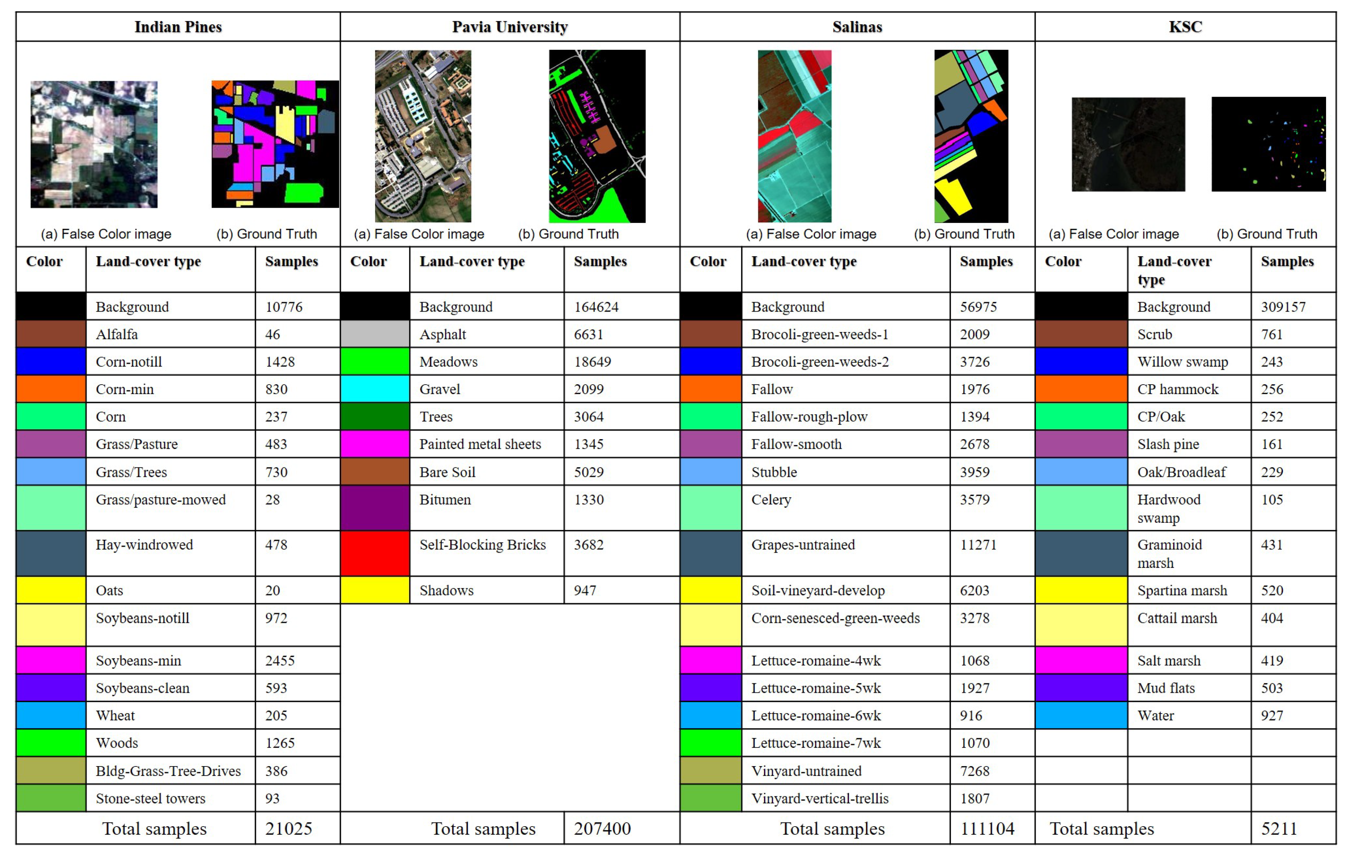
In our experiments, four well-known publicly available data sets, including Indian Pines, Pavia University, Salinas, and Kennedy Space Center, have been used to verify the effectiveness of SANet. Figure 6 shows a brief summary of these HSIs. The detailed information about them is given as follows.

3.1.1. Indian Pines

This image was gathered by the AVIRIS sensor over the Indian Pines test site in northwestern Indiana. This image comprises $145\times 145$ pixels, with a total of 224 spectral bands [61]. In addition, the spatial resolution is 20 meters per pixel (mpp). In our experiments, 200 spectral channels are retained by removing four null bands and 20 corrupted bands [62]. The name and quantity of each class are reported in the first column of Figure 6, where 10,249 samples contain ground truth information, and they belong to 16 different classes. HSI classification on this data set is challenging, due to the presence of mixed pixels and imbalanced class distribution [63].

3.1.2. Pavia University

The second image was recorded by the ROSIS sensor during a flight campaign over Pavia, northern Italy. The size of it is 610 × 340 × 115, and its spatial resolution is 1.3 mpp. In our experiments, 103 out of the 115 bands are kept after having removed 12 noisy bands. The total number of the labeled pixels is 42,776. In addition, these labeled pixels belong to 9 land-cover classes (see the second column of Figure 6).

3.1.3. Salinas

The third HSI used in experiments was acquired by the 224-band AVIRIS sensor over Salinas Valley, California. This image contains $512\times 217$ pixels with a spatial resolution of 3.7 mpp. After discarding the water absorption bands and noisy bands, there are 204 bands have been used in the experiments. A total of 54,129 pixels labeled in 16 classes are used for classification. Finally, the false color image and ground truth map are presented in the third column of Figure 6.

3.1.4. KSC

The last dataset was also acquired by the AVIRIS, but over the Kennedy Space Center (KSC), Florida, in 1996. Due to water absorption and the existence of low signal-noise ratio channels, 176 of them were used in our experiments. There are 13 land cover classes with 5211 labeled pixels. A three-band false color image and the ground-truth map are shown in Figure 6.

3.2. SANet Structure Analysis

The proposed SANet is a deep learning-based method. It can learn spectral-spatial features in a hierarchical way. Thus, the setting of the structure parameters of SANet plays an important role in feature learning. Here, we investigate how the depth and the number of scales in each layer influence the classification performance. In this section, only the experimental results on Indian Pines have been given, since we can make the same conclusions on other data sets. Here, only 2% labeled samples per class are used as training samples.

3.2.1. Depth Effect

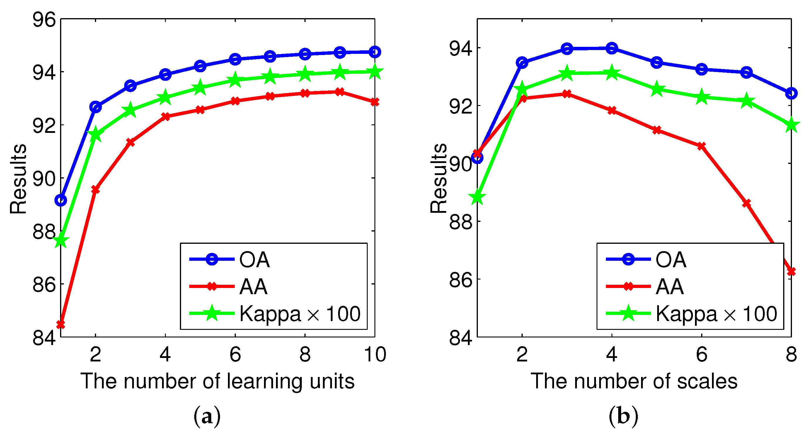
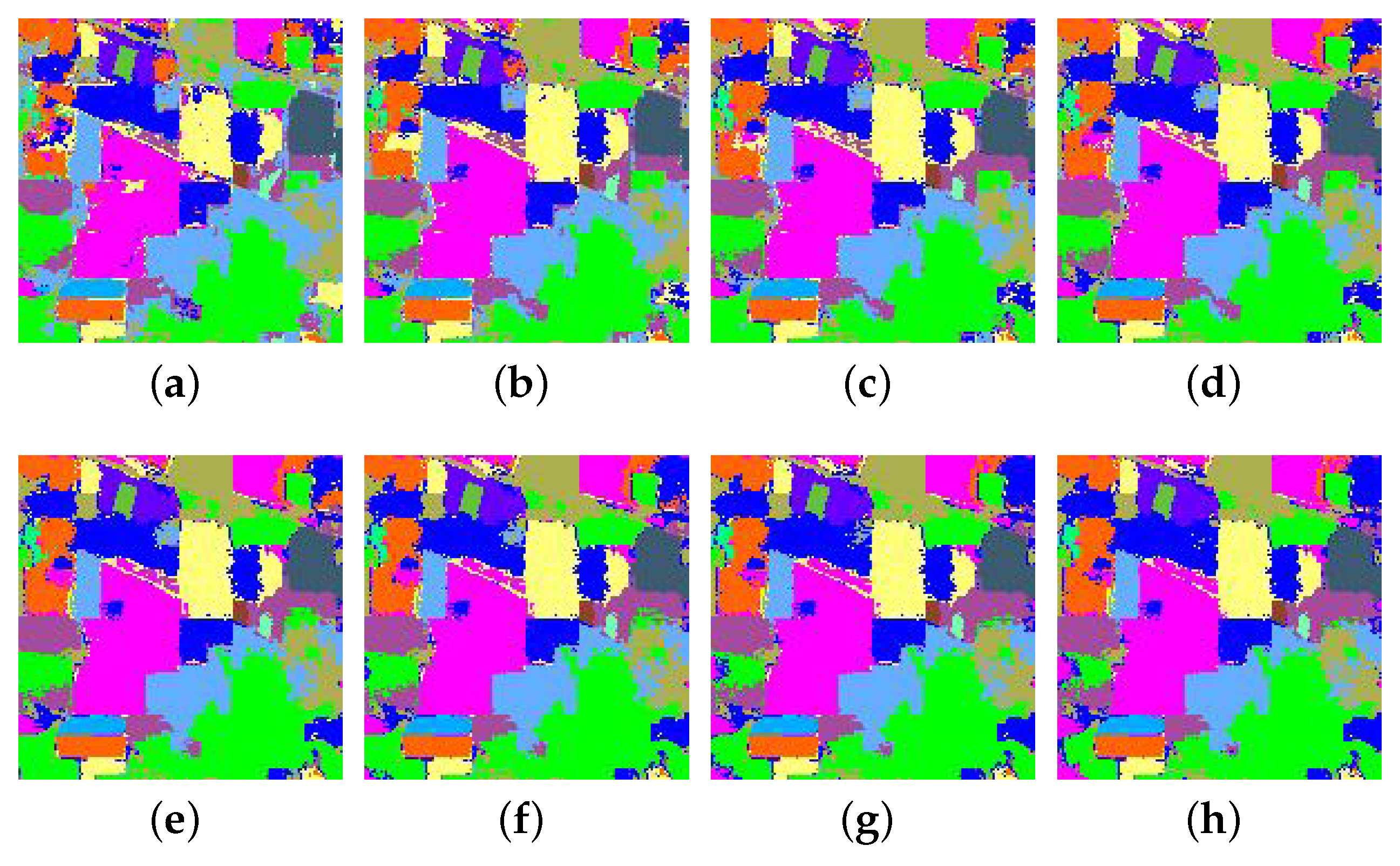
The depth of representations is of central importance for deep learning methods. In the proposed method, the depth determines the abstraction level of the learned spectral-spatial features. Consequently, extensive experiments have been conducted to show the relationship between the number of spectral-spatial learning units and the classification performance. In these experiments, we change only the depth and fix other parameters to investigate classification performance. Figure 7a and Figure 8 show the quantitative results and the classification maps with different depths. It is obvious that, with the increase of the depth, we will obtain better performance. However, it does not mean the deeper the better, which can be found from the curves in Figure 7a. Too deep layers could lead to over smoothing problems. Consequently, the number of the spectral-spatial feature learning units, which depicts the depth, is set to five for all data sets.

3.2.2. Scale Effect

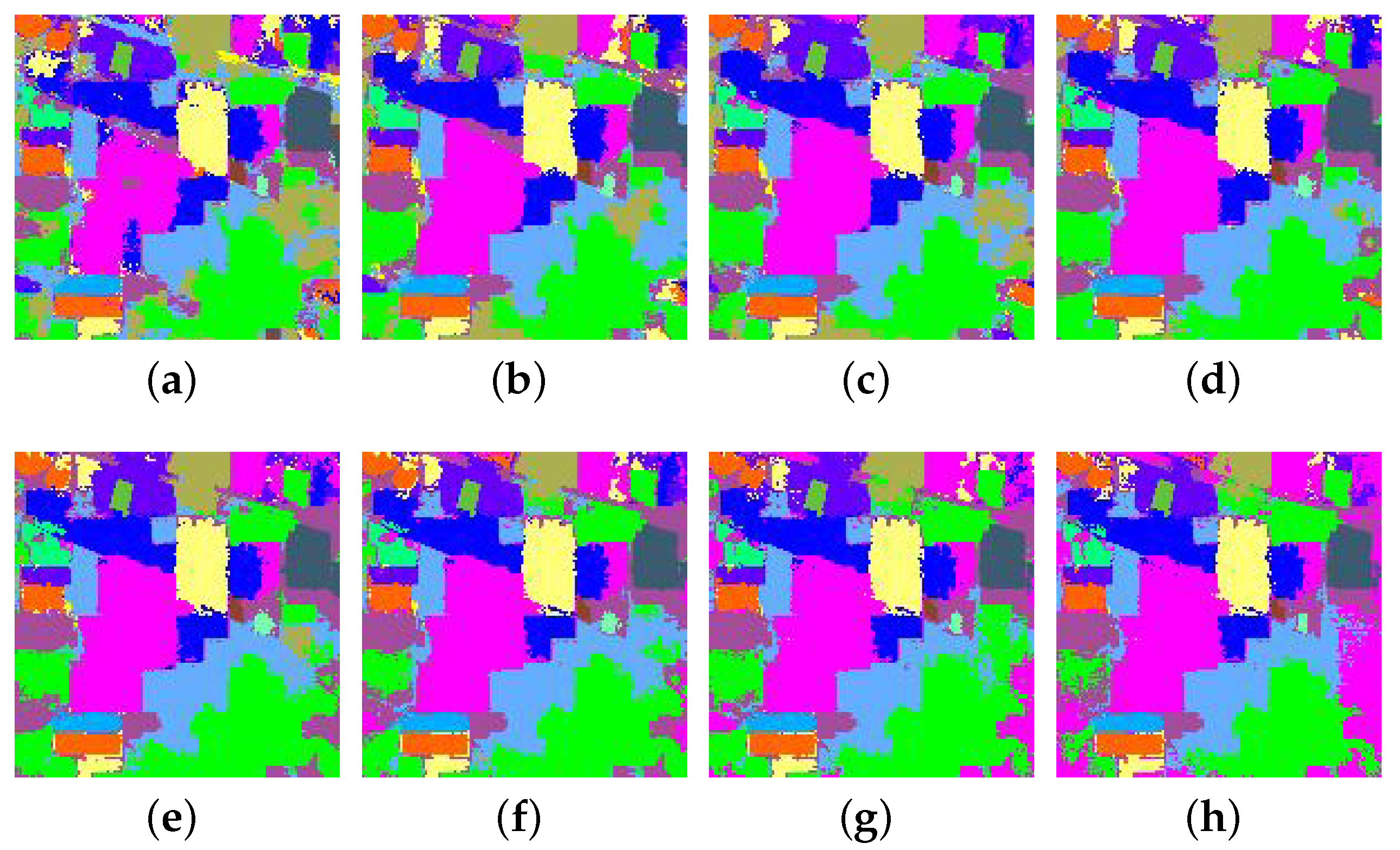
Multiscale is also an important factor related to the classification performance of SANet. The number of scales can also control the architecture or topology of the network. In order to show how to determine the number of scales, we change only the scale number in each layer and fix other parameters. As shown in Figure 7b, as the number of scales grows, the classification accuracies have a trend of rising first and then declining. We can see that SANet obtains the highest $\kappa$ coefficient when the number of scale is 3. Figure 9 also gives the classification maps corresponding to different scales. It can be observed that SANet obtains a better map when $\widehat{r}$ is set to 3. According to these observations, we experimentally set the number of scales, $\widehat{r}$, as 3 for all data sets. In this paper, the radii of side windows are set to {3, 5, 7}. A large scale number usually incurs high computational cost. Thus, it is also a trade-off between accuracy and computational expense to set $\widehat{r}$ as 3.

3.3. Comparison with State-of-the-Art Methods

In order to demonstrate the advantages of our SANet, we mainly consider the case of a small training set in this section.

3.3.1. Experimental Results on Indian Pines Data Set

The first experiment is conducted on an Indian Pines data set, where the number of training samples per class is set to be 2% of labeled samples, and the remaining samples are used for testing.

Table 1. Classification accuracies of HybridSN, STSE_DWLR, CNN-MRF, LCMR, RPNet, and SANet on the Indian Pines data set. The best results are highlighted in bold font.

No.	HybridSN	STSE_DWLR	CNN-MRF	LCMR	RPNet	SANet
1	17.78	97.78	46.67	96.67	14.67	97.56
2	70.29	82.47	70.33	91.54	86.90	92.49
3	71.87	85.23	67.75	84.06	69.43	89.82
4	70.69	82.28	43.36	77.72	26.21	78.58
5	83.30	79.41	78.94	93.51	83.62	88.88
6	97.76	97.23	85.69	95.58	90.69	98.36
7	48.15	60.00	36.30	100.0	70.74	99.26
8	99.57	100.0	92.46	100.0	84.81	99.94
9	0.000	13.68	69.47	74.21	41.58	62.11
10	79.22	83.74	63.03	83.61	78.68	88.63
11	91.77	96.13	87.88	92.44	95.92	96.26
12	54.73	79.35	59.52	83.80	48.43	89.35
13	78.11	98.41	71.05	97.15	89.10	99.30
14	96.53	97.89	95.05	96.71	92.17	99.95
15	63.76	98.44	57.27	93.04	55.63	91.64
16	75.82	88.79	80.77	80.44	29.67	99.01
OA	82.22	90.38	77.39	91.12	81.80	93.97
AA	68.71	83.80	69.10	90.03	66.14	91.95
$\kappa$	0.797	0.890	0.740	0.899	0.788	0.931

reports the quantitative results obtained by the proposed SANet and five state-of-the-art methods. Note that the best results are highlighted in bold font. We can observe that SANet achieves the best performance in terms of OA, AA, and $\kappa$. In addition, the proposed method obtains the best results on most of the classes. These experimental results also show that CNN-MRF achieves the lowest OA and $\kappa$ coefficient among six methods, mainly because CNN-MRF is directly trained with a small number of training samples, which may lead to overfitting problems. The OA, AA, and $\kappa$ of the CNN-MRF approach are 77.39%, 69.10%, and 0.740, respectively, while the results obtained by the proposed method are 93.97%, 91.95%, and 0.931, respectively. This indicates that the average improvement is more than 15%. LCMR achieves better results than HybridSN, STSE_DWLR, CNN-MRF, and RPNet, since it is a handcrafted feature extraction method designed for a small training set. However, the performance of the LCMR is still inferior to the proposed method. The main reason is that LCMR only considers the spectral-spatial features on single scale, while the proposed proposed method integrates multiscale spectral-spatial features using deep architecture.

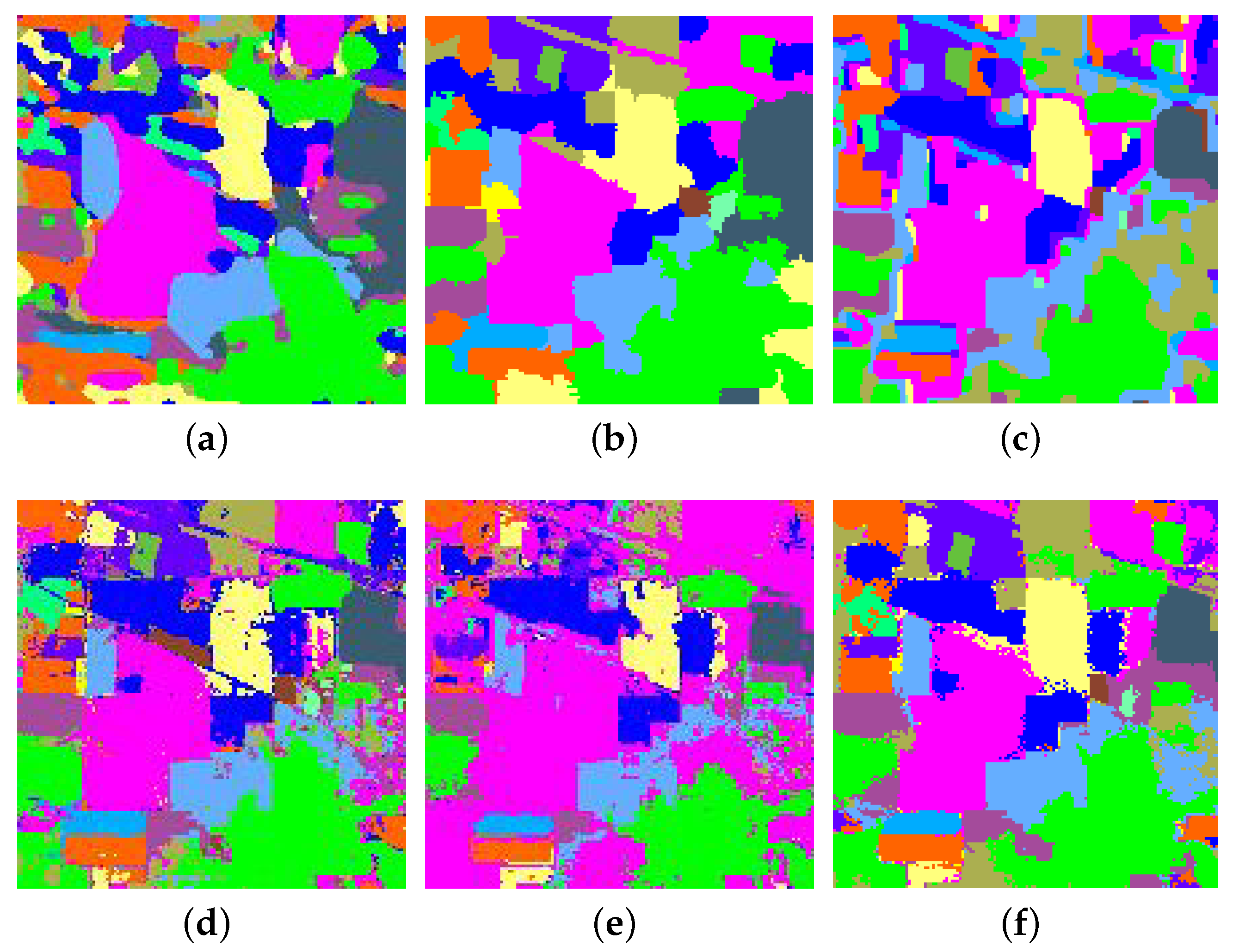
Apart from the quantitative comparisons, we also verify the effectiveness of the proposed method from a visual perspective. Figure 10 presents the full classification maps of different methods, and these maps are produced by one of the random experiments. We can easily observe that the proposed method obtains the best performance. HybridSN, STSE_DWLR, and CNN-MRF lead to oversmoothed classification maps. However, LCMR and RPNet always result in noisy classification maps. Our method can not only preserve the structures in accordance with the false color image (see Figure 6) but also produce smoother results. The main reasons for its good performance are threefold. First, by using a side window filtering principle, the edges and the boundaries of the HSI can be preserved, and the homogeneous regions can be smoothed. Second, the SANet can effectively exploit the spectral-spatial feature from different scales. Third, the LDA is used to remove the redundancy residing in the data, thus the proposed method can extract more discriminative features.

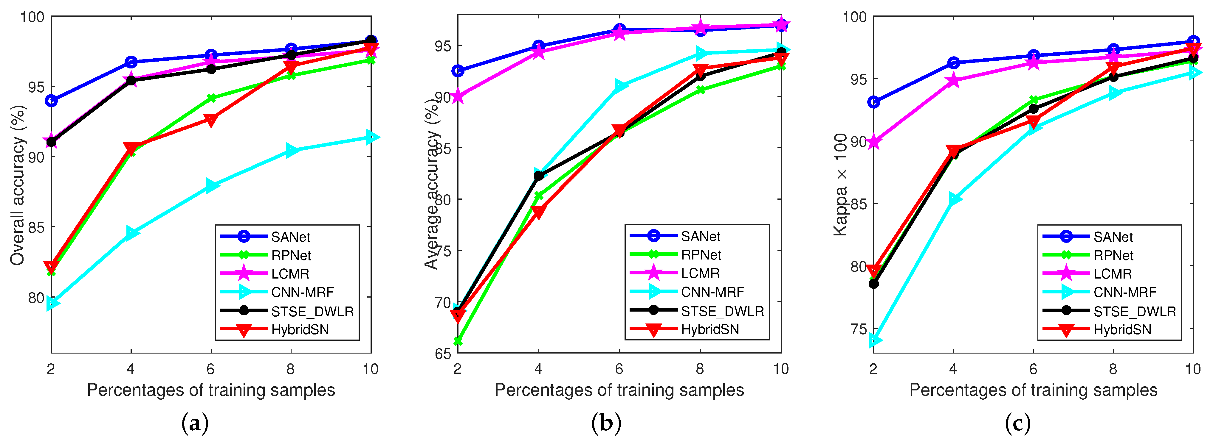
Furthermore, we analyze the effects of the number of training samples. We use 2%, 4%, 6%, 8%, and 10% randomly selected samples for each class in Indian Pines data set. We can make the observation from Figure 11 that the performance of the compared methods and the proposed method improve as the size of the training set increases. It is also noteworthy that SANet performs the best, especially when the number of training sample is small. This implies that the proposed approach is more suitable for HSI classification. Since the labeled samples are often difficult and expensive to be collected in practice.

Finally, the running times of different methods are presented in

Table 2. Running time of different methods on Indian Pines data set (S).

HybridSN	STSE_DWLR	CNN-MRF	LCMR	RPNet	SANet
170.18	26.15	438	9.59	5.82	11.73

. These results show that the proposed method has the low computational complexity, and the deep learning-based methods are time consuming. We can also make the same conclusion on other three data sets.

3.3.2. Experimental Results on Pavia University Data Set

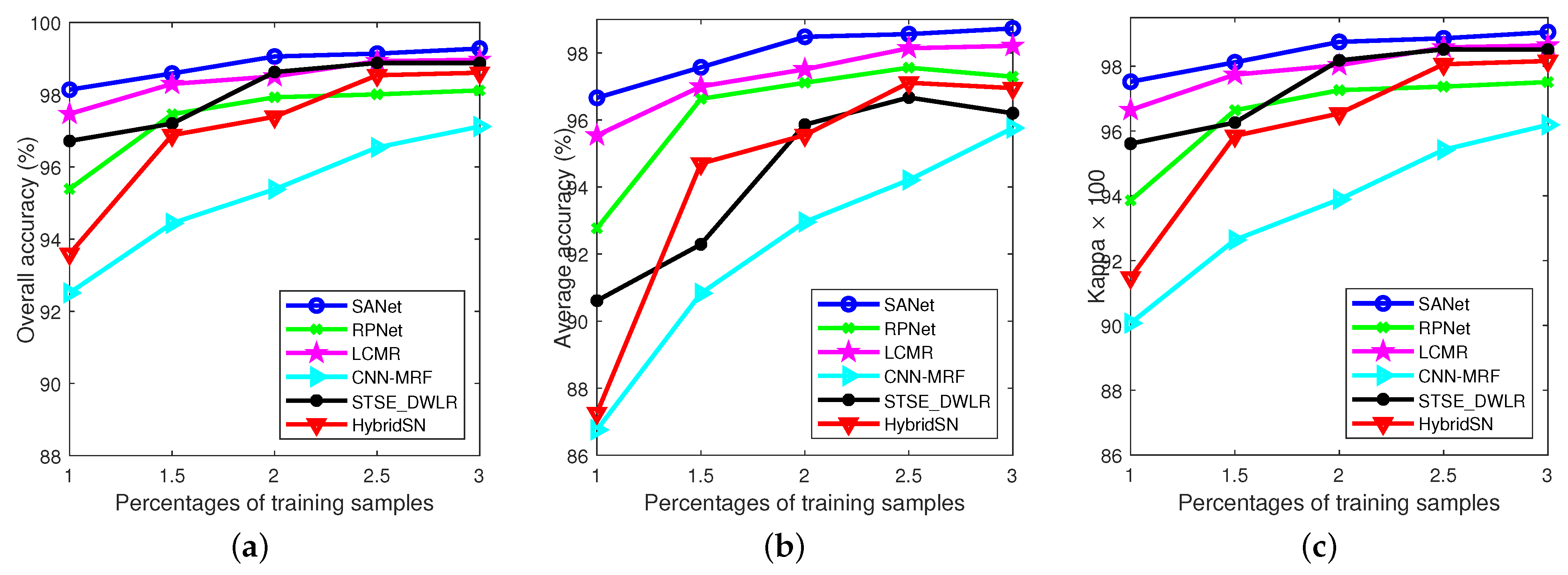
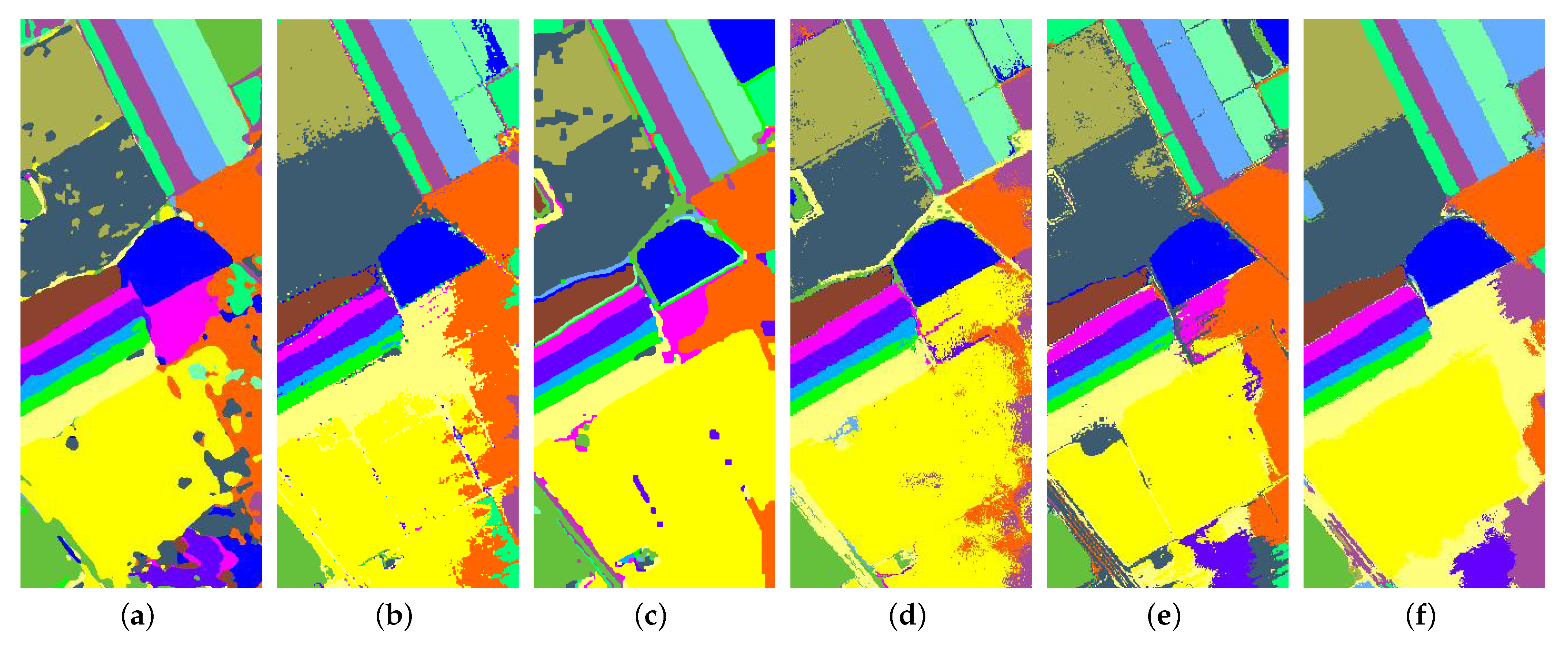
The second experiment is performed on the Pavia University data set (see Figure 6). In this case, 1% of labeled samples are randomly selected to form the training set.

Table 3. Classification accuracies of HybridSN, STSE_DWLR, CNN-MRF, LCMR, RPNet, and SANet on the Pavia University data set. The best results are highlighted in bold font.

No.	HybridSN	STSE_DWLR	CNN-MRF	LCMR	RPNet	SANet
1	90.78	99.84	93.79	95.82	91.40	98.55
2	99.84	99.98	98.51	99.53	97.94	99.85
3	71.80	99.83	65.04	92.23	86.48	92.54
4	73.95	74.82	95.95	98.25	91.23	92.38
5	98.05	99.62	96.66	97.81	95.51	99.69
6	99.86	100.0	93.15	99.14	93.83	99.21
7	99.62	99.98	64.00	94.75	81.66	96.95
8	92.24	97.97	80.21	92.97	87.40	95.93
9	59.23	43.48	93.55	89.36	96.03	94.87
OA	93.59	96.72	92.51	97.47	93.87	98.14
AA	87.26	90.61	86.76	95.54	91.28	96.67
$\kappa$	0.932	0.956	90.07	0.967	0.918	0.975

presents the quantitative results with respect to different metrics. We again conclude that SANet achieves the best performance compared with other state-of-the-art spectral-spatial methods. As can be seen, except for the proposed method, deep learning-based methods achieve the lower accuracies because of the limited training samples. Figure 12 visualizes the classification results of all the methods. We can observe in Figure 12b that STSE_DWLR leads to oversmoothing. In contrast, the proposed method can preserve the details of HSI. Figure 13 shows the influence of training samples size (ranging from 1% to 3%, with a step of 0.5% per class) on classification performance. Most of the compared methods achieve similar accuracies when the number of training samples is large enough. In contrast, the proposed method has obvious advantages in the case of small samples.

3.3.3. Experimental Results on the Salinas Data Set

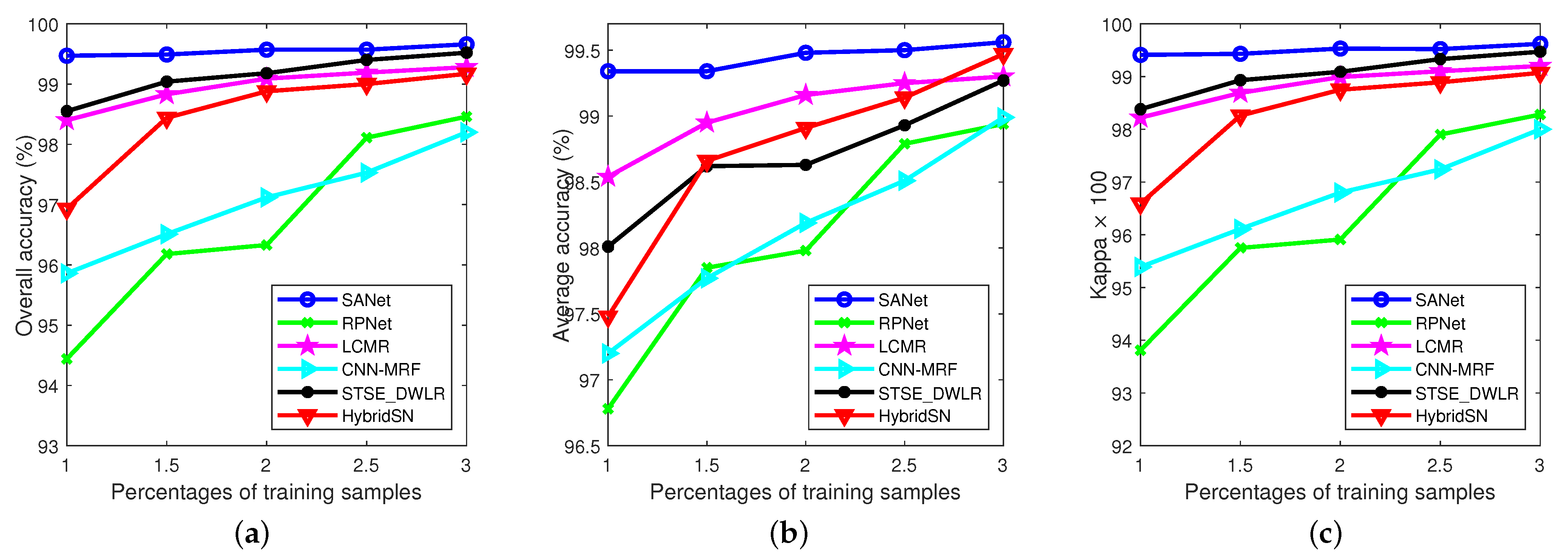
The third experiment is performed on the Salinas data set. Similar conclusions can be made from

Table 4. Classification accuracies of HybridSN, STSE_DWLR, CNN-MRF, LCMR, RPNet, and SANet on the Salinas data set. The best results are highlighted in bold font.

No.	HybridSN	STSE_DWLR	CNN-MRF	LCMR	RPNet	SANet
1	99.80	99.23	99.73	99.89	99.03	100.0
2	99.97	99.69	98.13	99.31	99.73	99.94
3	99.49	99.80	98.72	99.76	99.38	100.0
4	99.49	99.17	88.47	97.36	98.80	99.94
5	99.81	97.16	99.89	98.38	99.01	98.62
6	100.0	99.81	99.74	99.40	99.63	99.87
7	99.66	99.36	99.69	99.36	99.48	99.85
8	96.30	99.50	93.57	97.94	92.30	99.72
9	98.65	99.46	99.59	99.78	99.26	100.0
10	99.37	97.45	95.55	98.39	97.85	97.20
11	98.32	94.74	99.75	99.91	96.16	99.70
12	99.94	99.95	99.86	99.95	99.98	100.0
13	91.36	95.46	98.84	98.62	98.81	98.82
14	86.37	91.95	98.03	95.12	95.68	94.91
15	88.99	96.42	85.82	95.97	89.41	98.99
16	100.0	99.01	99.25	97.51	98.43	99.21
OA	96.34	98.55	95.86	98.40	96.31	99.39
AA	97.48	98.01	97.20	98.54	97.68	99.17
$\kappa$	0.966	0.984	0.954	0.982	0.959	0.993

and Figure 14, where 1% labeled samples are randomly selected per class for training. These results also demonstrate that the proposed SANet delivers the best performance in terms of OA, AA, and $\kappa$. Figure 14 also shows that HybridSN and CNN-MRF yield oversmoothed classification maps, while STSE_DWLR, LCMR and RPNet produce maps with much noise. Finally, Figure 15 shows the influence of the number of training samples (ranging from 1% to 3%, with a step of 0.5% per class) on the performance of the different methods. Similarly, we can conclude that the proposed method can achieve the best results with limited training samples. Furthermore, we can also find that all the methods show comparable performance only when enough training samples are available. This is due to the fact that conventional deep learning methods usually require a large number of training samples to obtain optimal parameter values.

3.3.4. Experimental Results on the KSC Data Set

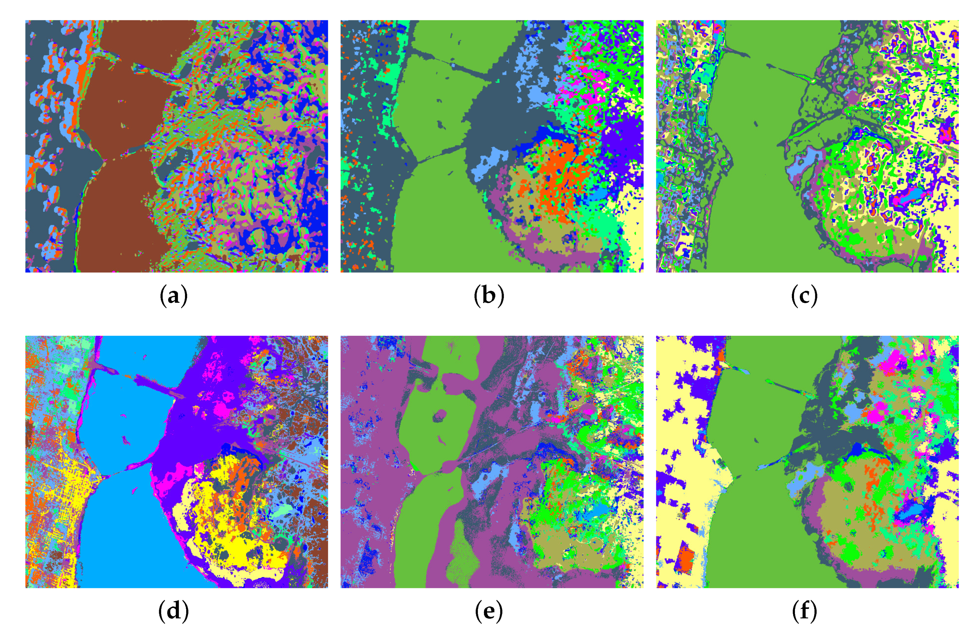
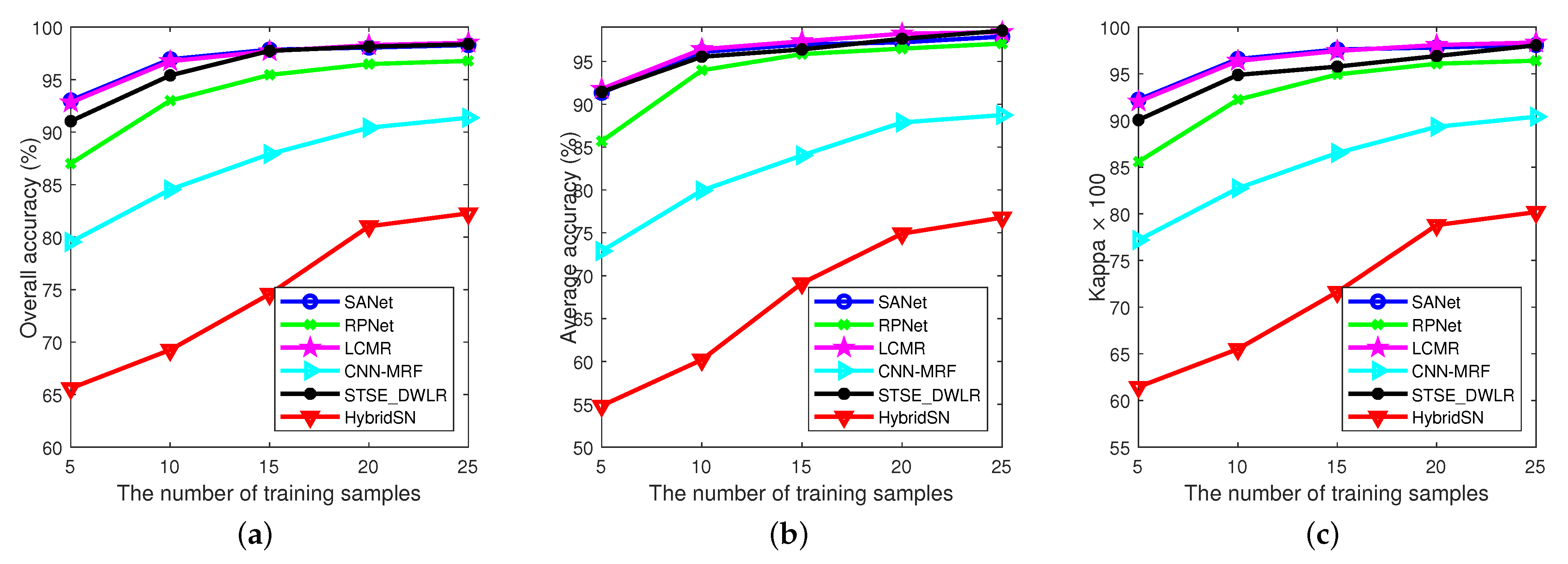
The fourth experiment is performed on the KSC data set. Similar conclusions can be made from

Table 5. Classification accuracies of HybridSN, STSE_DWLR, CNN-MRF, LCMR, RPNet, and SANet on the KSC data set. The best results are highlighted in bold font.

No.	HybridSN	STSE_DWLR	CNN-MRF	LCMR	RPNet	SANet
1	98.03	79.84	98.05	91.56	82.38	93.76
2	54.79	83.91	56.06	89.24	75.08	99.16
3	61.43	92.71	66.25	97.81	71.83	92.95
4	30.12	93.00	31.06	85.38	76.03	69.51
5	50.13	90.45	48.17	84.55	90.00	77.95
6	68.21	98.17	72.00	91.12	76.70	93.62
7	99.90	98.80	99.86	93.80	99.90	96.80
8	79.46	80.68	79.28	88.29	88.12	86.29
9	81.86	87.50	81.03	83.05	86.82	90.70
10	68.92	97.44	70.07	99.42	88.67	97.42
11	77.42	87.83	79.37	91.98	93.77	94.20
12	77.11	98.49	76.65	97.01	87.53	95.04
13	100.0	100.0	100.0	100.0	97.14	100.0
OA	79.53	91.04	79.55	92.83	87.01	93.02
AA	72.88	91.45	72.91	91.79	85.69	91.34
$\kappa$	0.7717	0.9005	0.7720	0.9203	0.8558	0.9223

and Figure 16, where five labeled samples are randomly selected per class for training. These results also demonstrate that the proposed SANet delivers the best performance in terms of OA, and $\kappa$. Figure 16 also shows that HybridSN and CNN-MRF yield oversmoothed classification maps, while LCMR and RPNet produce maps with much noise. Finally, Figure 17 shows the influence of the number of training samples (ranging from 5 to 25, with a step of 5 per class) on the performance of the different methods. Similarly, we can conclude that the proposed method can achieve the best results with limited training samples. Furthermore, we can also find that all the methods show comparable performance only when enough training samples are available. The reason for this is that conventional deep learning methods have high sample complexity.

To sum up, the experimental results on four typical data sets show that the proposed approach can provide better results than other tested methods. The proposed method can alleviate the potential overfitting problems that deep learning-based methods usually suffer when dealing with HSI classification.

4. Conclusions and Future Research

This paper develops an efficient deep spectral-spatial feature learning method for HSI classification. The proposed approach can obtain high accuracy with limited labeled samples by introducing the side window filtering principle to the deep feature learning, and integrating the spatial and the spectral information contained in the original HSIs. Our results also corroborate that incorporating prior domain knowledge into deep architecture can deal with the small sample problem in HSI classification. Future work will focus on improving the performance of the proposed method from the viewpoint of filtering, such as more effective filtering technology being able be applied to the side window filtering framework.

References

- Wan, S.; Gong, C.; Zhong, P.; Du, B.; Zhang, L.; Yang, J. Multiscale dynamic graph convolutional network for hyperspectral image classification. IEEE Trans. Geosci. Remote Sens. 2020, 58, 3162–3177. [Google Scholar] [CrossRef] [Green Version]
- Zhang, L.; Zhang, L.; Du, B. Deep learning for remote sensing data: A technical tutorial on the state of the art. IEEE Geosci. Remote Sens. Mag. 2016, 4, 22–40. [Google Scholar] [CrossRef]
- Goetz, A.F. Three decades of hyperspectral remote sensing of the Earth: A personal view. Remote Sens. Environ. 2009, 113, S5–S16. [Google Scholar] [CrossRef]
- Li, S.; Song, W.; Fang, L.; Chen, Y.; Ghamisi, P.; Benediktsson, J.A. Deep Learning for Hyperspectral Image Classification: An Overview. IEEE Trans. Geosci. Remote Sens. 2019, 57, 6690–6709. [Google Scholar] [CrossRef] [Green Version]
- Bioucas-Dias, J.M.; Plaza, A.; Camps-Valls, G.; Scheunders, P.; Nasrabadi, N.; Chanussot, J. Hyperspectral remote sensing data analysis and future challenges. IEEE Geosci. Remote Sens. Mag. 2013, 1, 6–36. [Google Scholar] [CrossRef] [Green Version]
- Zhang, X.; Sun, Y.; Shang, K.; Zhang, L.; Wang, S. Crop classification based on feature band set construction and object-oriented approach using hyperspectral images. IEEE J. Sel. Top. Appl. Earth Obs. Remote Sens. 2016, 9, 4117–4128. [Google Scholar] [CrossRef]
- Uzkent, B.; Rangnekar, A.; Hoffman, M. Aerial vehicle tracking by adaptive fusion of hyperspectral likelihood maps. In Proceedings of the IEEE Conference on Computer Vision and Pattern Recognition Workshops, Honolulu, HI, USA, 21–26 July 2017; pp. 39–48. [Google Scholar]
- He, X.; Chen, Y.; Lin, Z. Spatial-Spectral Transformer for Hyperspectral Image Classification. Remote Sens. 2021, 13, 498. [Google Scholar] [CrossRef]
- Yang, W.; Peng, J.; Sun, W.; Du, Q. Log-Euclidean Kernel-Based Joint Sparse Representation for Hyperspectral Image Classification. IEEE J. Sel. Top. Appl. Earth Obs. Remote Sens. 2019, 12, 5023–5034. [Google Scholar] [CrossRef]
- Ma, Y.; Zhang, Y.; Mei, X.; Dai, X.; Ma, J. Multifeature-Based Discriminative Label Consistent K-SVD for Hyperspectral Image Classification. IEEE J. Sel. Top. Appl. Earth Obs. Remote Sens. 2019, 12, 4995–5008. [Google Scholar] [CrossRef]
- Signoroni, A.; Savardi, M.; Baronio, A.; Benini, S. Deep Learning Meets Hyperspectral Image Analysis: A Multidisciplinary Review. J. Imaging 2019, 5, 52. [Google Scholar] [CrossRef] [Green Version]
- Audebert, N.; Le Saux, B.; Lefèvre, S. Deep Learning for Classification of Hyperspectral Data: A Comparative Review. IEEE Geosci. Remote Sens. Mag. 2019, 7, 159–173. [Google Scholar] [CrossRef] [Green Version]
- Kang, X.; Zhuo, B.; Duan, P. Dual-path network-based hyperspectral image classification. IEEE Geosci. Remote Sens. Lett. 2018, 16, 447–451. [Google Scholar] [CrossRef]
- Jia, S.; Deng, X.; Zhu, J.; Xu, M.; Zhou, J.; Jia, X. Collaborative representation-based multiscale superpixel fusion for hyperspectral image classification. IEEE Trans. Geosci. Remote Sens. 2019, 57, 7770–7784. [Google Scholar] [CrossRef]
- Tu, B.; Wang, J.; Zhang, G.; Zhang, X.; He, W. Texture Pattern Separation for Hyperspectral Image Classification. IEEE J. Sel. Top. Appl. Earth Obs. Remote Sens. 2019, 12, 3602–3614. [Google Scholar] [CrossRef]
- Pan, B.; Shi, Z.; Xu, X. MugNet: Deep learning for hyperspectral image classification using limited samples. ISPRS J. Photogramm. Remote Sens. 2018, 145, 108–119. [Google Scholar] [CrossRef]
- Luo, F.; Zhang, L.; Du, B.; Zhang, L. Dimensionality reduction with enhanced hybrid-graph discriminant learning for hyperspectral image classification. IEEE Trans. Geosci. Remote Sens. 2020, 58, 5336–5353. [Google Scholar] [CrossRef]
- Plaza, A.; Martinez, P.; Plaza, J.; Perez, R. Dimensionality reduction and classification of hyperspectral image data using sequences of extended morphological transformations. IEEE Trans. Geosci. Remote Sens. 2005, 43, 466–479. [Google Scholar] [CrossRef] [Green Version]
- Chang, C.I.; Du, Q.; Sun, T.L.; Althouse, M.L. A joint band prioritization and band-decorrelation approach to band selection for hyperspectral image classification. IEEE Trans. Geosci. Remote Sens. 1999, 37, 2631–2641. [Google Scholar] [CrossRef] [Green Version]
- Ghamisi, P.; Maggiori, E.; Li, S.; Souza, R.; Tarablaka, Y.; Moser, G.; De Giorgi, A.; Fang, L.; Chen, Y.; Chi, M.; et al. New frontiers in spectral-spatial hyperspectral image classification: The latest advances based on mathematical morphology, Markov random fields, segmentation, sparse representation, and deep learning. IEEE Geosci. Remote Sens. Mag. 2018, 6, 10–43. [Google Scholar] [CrossRef]
- He, N.; Paoletti, M.E.; Haut, J.M.; Fang, L.; Li, S.; Plaza, A.; Plaza, J. Feature extraction with multiscale covariance maps for hyperspectral image classification. IEEE Trans. Geosci. Remote Sens. 2019, 57, 755–769. [Google Scholar] [CrossRef]
- He, L.; Li, J.; Liu, C.; Li, S. Recent advances on spectral–spatial hyperspectral image classification: An overview and new guidelines. IEEE Trans. Geosci. Remote Sens. 2018, 56, 1579–1597. [Google Scholar] [CrossRef]
- Li, W.; Du, Q. Gabor-filtering-based nearest regularized subspace for hyperspectral image classification. IEEE J. Sel. Top. Appl. Earth Obs. Remote Sens. 2014, 7, 1012–1022. [Google Scholar] [CrossRef]
- Benediktsson, J.A.; Palmason, J.A.; Sveinsson, J.R. Classification of hyperspectral data from urban areas based on extended morphological profiles. IEEE Trans. Geosci. Remote Sens. 2005, 43, 480–491. [Google Scholar] [CrossRef]
- He, L.; Li, J.; Plaza, A.; Li, Y. Discriminative low-rank Gabor filtering for spectral–spatial hyperspectral image classification. IEEE Trans. Geosci. Remote Sens. 2016, 55, 1381–1395. [Google Scholar] [CrossRef]
- Kang, X.; Li, S.; Benediktsson, J.A. Spectral–spatial hyperspectral image classification with edge-preserving filtering. IEEE Trans. Geosci. Remote Sens. 2014, 52, 2666–2677. [Google Scholar] [CrossRef]
- Li, J.; Bioucas-Dias, J.M.; Plaza, A. Spectral–spatial hyperspectral image segmentation using subspace multinomial logistic regression and Markov random fields. IEEE Trans. Geosci. Remote Sens. 2012, 50, 809–823. [Google Scholar] [CrossRef]
- Zhong, P.; Wang, R. Jointly learning the hybrid CRF and MLR model for simultaneous denoising and classification of hyperspectral imagery. IEEE Trans. Neural Netw. Learn. Syst. 2014, 25, 1319–1334. [Google Scholar] [CrossRef]
- Li, C.; Ma, Y.; Mei, X.; Liu, C.; Ma, J. Hyperspectral image classification with robust sparse representation. IEEE Geosci. Remote Sens. Lett. 2016, 13, 641–645. [Google Scholar] [CrossRef]
- Jia, S.; Zhang, X.; Li, Q. Spectral–Spatial Hyperspectral Image Classification Using l1/2 Regularized Low-Rank Representation and Sparse Representation-Based Graph Cuts. IEEE J. Sel. Top. Appl. Earth Obs. Remote Sens. 2015, 8, 2473–2484. [Google Scholar] [CrossRef]
- Chen, C.; Chen, N.; Peng, J. Nearest regularized joint sparse representation for hyperspectral image classification. IEEE Geosci. Remote Sens. Lett. 2016, 13, 424–428. [Google Scholar] [CrossRef]
- Wei, Y.; Zhou, Y.; Li, H. Spectral-Spatial Response for Hyperspectral Image Classification. Remote Sens. 2017, 9, 203. [Google Scholar] [CrossRef] [Green Version]
- Zhou, Y.; Wei, Y. Learning hierarchical spectral–spatial features for hyperspectral image classification. IEEE Trans. Cybern. 2016, 46, 1667–1678. [Google Scholar] [CrossRef]
- Peng, J.; Li, L.; Tang, Y.Y. Maximum likelihood estimation-based joint sparse representation for the classification of hyperspectral remote sensing images. IEEE Trans. Neural Netw. Learn. Syst. 2018, 30, 1790–1802. [Google Scholar] [CrossRef] [PubMed]
- Peng, J.; Jiang, X.; Chen, N.; Fu, H. Local adaptive joint sparse representation for hyperspectral image classification. Neurocomputing 2019, 334, 239–248. [Google Scholar] [CrossRef]
- Xu, Y.; Du, B.; Zhang, L. Beyond the Patchwise Classification: Spectral-Spatial Fully Convolutional Networks for Hyperpsectral Image Classificaiton. IEEE Trans. Big Data 2020, 6, 492–506. [Google Scholar] [CrossRef]
- Jiang, J.; Chen, C.; Yu, Y.; Jiang, X.; Ma, J. Spatial-aware collaborative representation for hyperspectral remote sensing image classification. IEEE Geosci. Remote Sens. Lett. 2017, 14, 404–408. [Google Scholar] [CrossRef]
- Tarabalka, Y.; Chanussot, J.; Benediktsson, J.A. Segmentation and classification of hyperspectral images using watershed transformation. Pattern Recognit. 2010, 43, 2367–2379. [Google Scholar] [CrossRef] [Green Version]
- Tu, B.; Kuang, W.; Zhao, G.; Fei, H. Hyperspectral image classification via superpixel spectral metrics representation. IEEE Signal Process. Lett. 2018, 25, 1520–1524. [Google Scholar] [CrossRef]
- Zheng, C.; Wang, N.; Cui, J. Hyperspectral image classification with small training sample size using superpixel-guided training sample enlargement. IEEE Trans. Geosci. Remote Sens. 2019, 57, 7307–7316. [Google Scholar] [CrossRef]
- Zehtabian, A.; Ghassemian, H. Automatic object-based hyperspectral image classification using complex diffusions and a new distance metric. IEEE Trans. Geosci. Remote Sens. 2016, 54, 4106–4114. [Google Scholar] [CrossRef]
- Deng, C.; Xue, Y.; Liu, X.; Li, C.; Tao, D. Active transfer learning network: A unified deep joint spectral–spatial feature learning model for hyperspectral image classification. IEEE Trans. Geosci. Remote Sens. 2019, 57, 1741–1754. [Google Scholar] [CrossRef] [Green Version]
- Shrestha, A.; Mahmood, A. Review of Deep Learning Algorithms and Architectures. IEEE Access 2019, 7, 53040–53065. [Google Scholar] [CrossRef]
- Kang, X.; Li, C.; Li, S.; Lin, H. Classification of hyperspectral images by Gabor filtering based deep network. IEEE J. Sel. Top. Appl. Earth Obs. Remote Sens. 2018, 11, 1166–1178. [Google Scholar] [CrossRef]
- Hang, R.; Liu, Q.; Hong, D.; Ghamisi, P. Cascaded recurrent neural networks for hyperspectral image classification. IEEE Trans. Geosci. Remote Sens. 2019, 57, 5384–5394. [Google Scholar] [CrossRef] [Green Version]
- Chen, Y.; Lin, Z.; Zhao, X.; Wang, G.; Gu, Y. Deep learning-based classification of hyperspectral data. IEEE J. Sel. Top. Appl. Earth Obs. Remote Sens. 2014, 7, 2094–2107. [Google Scholar] [CrossRef]
- Chen, Y.; Zhao, X.; Jia, X. Spectral–spatial classification of hyperspectral data based on deep belief network. IEEE J. Sel. Top. Appl. Earth Obs. Remote Sens. 2015, 8, 2381–2392. [Google Scholar] [CrossRef]
- Cao, X.; Zhou, F.; Xu, L.; Meng, D.; Xu, Z.; Paisley, J. Hyperspectral image classification with Markov random fields and a convolutional neural network. IEEE Trans. Image Process. 2018, 27, 2354–2367. [Google Scholar] [CrossRef] [PubMed] [Green Version]
- Yang, X.; Ye, Y.; Li, X.; Lau, R.Y.; Zhang, X.; Huang, X. Hyperspectral image classification with deep learning models. IEEE Trans. Geosci. Remote Sens. 2018, 56, 5408–5423. [Google Scholar] [CrossRef]
- Zhu, L.; Chen, Y.; Ghamisi, P.; Benediktsson, J.A. Generative adversarial networks for hyperspectral image classification. IEEE Trans. Geosci. Remote Sens. 2018, 56, 5046–5063. [Google Scholar] [CrossRef]
- Fang, L.; He, N.; Li, S.; Plaza, A.J.; Plaza, J. A new spatial–spectral feature extraction method for hyperspectral images using local covariance matrix representation. IEEE Trans. Geosci. Remote Sens. 2018, 56, 3534–3546. [Google Scholar] [CrossRef]
- Xu, Y.; Du, B.; Zhang, F.; Zhang, L. Hyperspectral image classification via a random patches network. ISPRS J. Photogramm. Remote Sens. 2018, 142, 344–357. [Google Scholar] [CrossRef]
- Muralidhar, N.; Islam, M.R.; Marwah, M.; Karpatne, A.; Ramakrishnan, N. Incorporating Prior Domain Knowledge into Deep Neural Networks. In Proceedings of the 2018 IEEE International Conference on Big Data (Big Data), Seattle, WA, USA, 10–13 December 2018; pp. 36–45. [Google Scholar]
- Pan, B.; Shi, Z.; Xu, X. Hierarchical guidance filtering-based ensemble classification for hyperspectral images. IEEE Trans. Geosci. Remote Sens. 2017, 55, 4177–4189. [Google Scholar] [CrossRef]
- Kang, X.; Xiang, X.; Li, S.; Benediktsson, J.A. PCA-based edge-preserving features for hyperspectral image classification. IEEE Trans. Geosci. Remote Sens. 2017, 55, 7140–7151. [Google Scholar] [CrossRef]
- Della Porta, C.J.; Bekit, A.A.; Lampe, B.H.; Chang, C.I. Hyperspectral Image Classification via Compressive Sensing. IEEE Trans. Geosci. Remote Sens. 2019, 57, 8290–8303. [Google Scholar] [CrossRef]
- Yin, H.; Gong, Y.; Guoping, Q. Side Window Filtering. In Proceedings of the IEEE Conference on Computer Vision and Pattern Recognition, Long Beach, CA, USA, 16–20 June 2019; pp. 147–156. [Google Scholar]
- Du, C.; Wang, Y.; Wang, C.; Shi, C.; Xiao, B. Selective feature connection mechanism: Concatenating multi-layer cnn features with a feature selector. Pattern Recognit. Lett. 2020, 129, 108–114. [Google Scholar] [CrossRef]
- Roy, S.K.; Krishna, G.; Dubey, S.R.; Chaudhuri, B.B. HybridSN: Exploring 3D-2D CNN Feature Hierarchy for Hyperspectral Image Classification. IEEE Geosci. Remote Sens. Lett. 2019, 17, 492–506. [Google Scholar]
- Pu, H.; Chen, Z.; Wang, B.; Jiang, G.M. A Novel Spatial–Spectral Similarity Measure for Dimensionality Reduction and Classification of Hyperspectral Imagery. IEEE Trans. Geosci. Remote Sens. 2014, 52, 7008–7022. [Google Scholar]
- Paoletti, M.E.; Haut, J.M.; Fernandez-Beltran, R.; Plaza, J.; Plaza, A.J.; Pla, F. Deep pyramidal residual networks for spectral–spatial hyperspectral image classification. IEEE Trans. Geosci. Remote Sens. 2019, 57, 740–754. [Google Scholar] [CrossRef]
- Haut, J.M.; Paoletti, M.E.; Plaza, J.; Li, J.; Plaza, A. Active learning with convolutional neural networks for hyperspectral image classification using a new bayesian approach. IEEE Trans. Geosci. Remote Sens. 2018, 56, 6440–6461. [Google Scholar] [CrossRef]
- Li, J.; Bioucas-Dias, J.M.; Plaza, A. Spectral-spatial classification of hyperspectral data using loopy belief propagation and active learning. IEEE Trans. Geosci. Remote Sens. 2013, 51, 844–856. [Google Scholar] [CrossRef]
Figure 1.
Schematic diagram of the proposed SANet, where only six hidden layers have been given for simplicity.
Figure 2.
Definition of the SWF.
Figure 3.
(a) The left and right side windows; (b) the up and down side windows; (c) the northwest, northeast, southwest, and southeast side windows.
Figure 4.
Multiscale filtering on band i, where feature maps have been derived from one band.
Figure 5.
MIN pooling on the rth scale corresponding to band i. For the ith band, each scale can produce one feature map.
Figure 6.
Details of the Indian Pines, Pavia University, and Salinas HSI data sets. They include the false color images, ground truths, and numbers of samples per class.
Figure 7.
Effect of using different numbers of (a) learning units and (b) scales.
Figure 8.
Full classification maps of Indian Pines data set using different numbers of learning units. (a) one unit; (b) two units; (c) three units; (d) four units; (e) five units; (f) six units; (g) seven units; (h) eight units.
Figure 9.
Full classification maps of Indian Pines data set using different numbers of scales. (a) one scale; (b) two scales; (c) three scales; (d) four scales; (e) five scales; (f) six scales; (g) seven scales; (h) eight scales.
Figure 10.
Classification maps for the Indian Pines data set using different methods. (a) HybridSN; (b) STSE_DWLR; (c) CNN-MRF; (d) LCMR; (e) RPNet; (f) SANet.
Figure 11.
Experimental results of different methods with various numbers of training samples on Indian Pines data set. (a) OAs; (b) AAs; (c) coefficients.
Figure 12.
Classification maps for the University of Pavia data set using different methods. (a) HybridSN; (b) STSE_DWLR; (c) CNN-MRF; (d) LCMR; (e) RPNet; (f) SANet.
Figure 13.
Experimental results of different methods with various numbers of training samples on Pavia University data set. (a) OAs; (b) AAs; (c) coefficients.
Figure 14.
Classification maps for the Salinas data set using different methods. (a) HybridSN; (b) STSE_DWLR; (c) CNN-MRF; (d) LCMR; (e) RPNet; (f) SANet.
Figure 15.
Experimental results of different methods with various numbers of training samples on Salinas data set. (a) OAs; (b) AAs; (c) coefficients.
Figure 16.
Classification maps for the Center of KSC data set using different methods. (a) HybridSN; (b) STSE_DWLR; (c) CNN-MRF; (d) LCMR; (e) RPNet; (f) SANet.
Figure 17.
Experimental results of different methods with various numbers of training samples on KSC data set. (a) OAs; (b) AAs; (c) coefficients.