Article

Mapping Regional Soil Organic Matter Based on Sentinel-2A and MODIS Imagery Using Machine Learning Algorithms and Google Earth Engine

1
School of Public Administration and Law, Northeast Agricultural University, Harbin 150030, China
2
Department of Earth System Science, Tsinghua University, Beijing 100089, China
3
Key Laboratory of Forest Ecology and Environment of State Forestry Administration, Institute of Forest Ecology, Environment and Protection, Chinese Academy of Forestry, Beijing 100091, China
4
College of Surveying and Geo-Informatics, Tongji University, Shanghai 200092, China
5
School of Environment, Tsinghua University, Beijing 100089, China
6
Northeast Institute of Geography and Agroecology, Chinese Academy of Sciences, Changchun 130012, China
*
Author to whom correspondence should be addressed.
Remote Sens. 2021, 13(15), 2934; https://doi.org/10.3390/rs13152934
Submission received: 22 June 2021 / Revised: 21 July 2021 / Accepted: 22 July 2021 / Published: 26 July 2021

Abstract

:
Many studies have attempted to predict soil organic matter (SOM), whereas mapping high-precision and high-resolution SOM maps remains a challenge due to the difficulty of selecting appropriate satellite data sources and prediction algorithms. This study aimed to investigate the influence of different remotely sensed images and machine learning algorithms on SOM prediction. We constructed two comparative experiments, i.e., full-band and common-band variable datasets of Sentinel-2A and MODIS images using Google Earth Engine (GEE). The predictive performances of random forest (RF), artificial neural network (ANN), and support vector regression (SVR) algorithms were evaluated, and the SOM map was generated for the Songnen Plain. Results showed that the model based on the full-band Sentinel-2A dataset achieved the best performance. The application of Sentinel-2A data resulted in mean relative improvements (RIs) of 7.67% and 5.87%, respectively. The RF achieved a lower root mean squared error (RMSE = 0.68%) and a higher coefficient of determination (R2 = 0.67) in all of the predicted scenarios than ANN and SVR. The resultant SOM map accurately characterized the SOM spatial distribution. Therefore, the Sentinel-2A data have obvious advantages over MODIS due to their higher spectral and spatial resolutions, and the combination of the RF algorithm and GEE is an effective approach to SOM mapping.

Graphical Abstract

1. Introduction

Soil is an integral part of terrestrial ecosystems and plays a vital role in the circulation of energy and materials between the atmosphere and the biosphere [1,2]. Soil organic matter (SOM) is an important component of soil that affects soil fertility and carbon sequestration [3,4,5,6,7] and plays an important role in improving crop yield [8,9,10] and maintaining agricultural sustainability and food security [11]. Therefore, accurately predicting and quantifying the spatial distribution of SOM is vital for promoting the improvement of soil fertility, the development of a sustainable regional ecosystem, and the implementation of soil management policies [12]. Although many studies have been done on building SOM prediction models and accomplishing mapping of spatial distribution, it remains a challenge to accurately map SOM content due to the difficulty of selecting appropriate satellite data sources and prediction algorithms for a specific region.
Numerous methods have been developed to map the spatial distribution of SOM. The traditional approach applies a titration procedure [13] to soil samples in a spectrophotometer [14] to determine the SOM content. However, it is difficult to quantitatively obtain the SOM spatial distribution at large scales [15] because large amounts of time and money are required to conduct soil survey activities; moreover, the measured SOM values are significantly affected by the field experience of the soil surveyor [16,17]. Subsequently, geostatistical methods [18] (e.g., kriging and cokriging) are widely applied to predict SOM [12,19,20,21,22,23]. However, these methods require the collection of sufficiently dense [23,24,25,26] and representative soil samples [27], as well as the assumption of second-order stationarity [28,29]. With the rapid development of remote sensing technology, SOM prediction approaches based on satellite remote sensing data have undergone significant development. Early SOM remote sensing prediction relied mainly on linear regression analysis [12,30,31,32,33]. Currently, various empirical models have been gradually developed and have exhibited improved prediction accuracy [34,35]. These models generally associate different statistical methods with predictive variables that are closely related to the SOM content [35,36], such as combining remote sensing data with topographical data. However, it is worth noting that problems of nonlinearity and multicollinearity exist in the kriging and multiple linear regression calculation processes [37,38,39,40].
To overcome these restrictions, the application of machine learning algorithms, such as random forest (RF) [41,42,43,44,45], artificial neural network (ANN) [23,26,29,40,46,47], and support vector regression (SVR) [11,48,49] algorithms, has gradually developed in soil science research due to the significant advantages of these algorithms over previous approaches, i.e., improved model accuracy, greater computing efficiency, and simplified fitting. Due to the spatial variability in climatic conditions, soil parent materials, human activities, and land use management, no single algorithm model is universally applicable for predicting SOM in different regions [50,51]. Some researchers have tried to compare the SOM prediction performances of multiple algorithms [11,52]. However, most of the existing studies in Northeast China have explored SOM prediction accuracy generally based on a single algorithm and a single type of satellite imagery [53,54,55,56,57] or on hyperspectral satellite data [58,59]. Therefore, the combination of different machine learning algorithms with multiple satellite images for SOM prediction must be further explored.
Thus far, many studies have suggested that SOM is sensitive over the entire visible near-infrared (VNIR)-shortwave infrared (SWIR) (400–2500 nm) region [60,61,62]. The SOM content can be reflected by differences in the spectral reflectance characteristics of soil [63,64,65]. A great deal of work has been done in applying remote sensing images to establish prediction models for soil properties and to complete the mapping of the spatial distribution of soil properties by using sensitive bands or spectral indices as model input variables; this is particularly common with Moderate Resolution Imaging Spectroradiometer (MODIS) products (e.g., MOD09A1 images) [50,54,66,67]. However, MOD09A1 pixels frequently include data from different dates during the eight-day composite period [54], and the pixels may simultaneously reflect abnormal conditions in local areas caused by other environmental factors (e.g., atmospheric conditions and crop residue); these issues arise due to the limitation of the moderate spatial resolution of the sensor and thereby limit the potential improvement of SOM prediction accuracy.
To overcome the heterogeneity of MODIS pixels, it is thus important to use remotely sensed data with higher spectral and spatial resolutions to ensure reasonable SOM prediction accuracy and produce high-precision spatial distribution maps. The Sentinel-2A satellite performs multispectral imaging missions with high spatial resolution and includes 13 bands in the visible, near-infrared (NIR), and shortwave infrared (SWIR) regions of the spectrum. The use of Sentinel-2A data significantly improves the spatial resolution of observations and provides an effective solution to the problems of the low availability and spatial resolution of MODIS data. Therefore, it is necessary to evaluate the application potential of Sentinel-2A data for SOM prediction to supplement the insufficiency of the information contained in MODIS data and to draw high-precision spatial distribution maps.
To our knowledge, relatively little is understood about the underlying relationships between the spatial distribution of SOM and the separate use of time series Sentinel-2A and MODIS images derived from the Google Earth Engine (GEE) data pool with three machine learning algorithms (i.e., RF, ANN, and SVR). Hence, our study was undertaken with the following objectives: (1) to compare the performances of Sentinel-2A and MODIS data for SOM prediction; (2) to compare the performances of models based on different machine learning algorithms for regional-scale SOM prediction; and (3) to map the spatial distribution patterns of SOM content in the cultivated areas of the Songnen Plain.

2. Materials and Methods

Figure 1 shows a comprehensive overview of the methods applied to map SOM in the Songnen Plain. The major parts are as follows: the yellow panels collect field samplings and build the training and validation sample sets; the purple panels construct two sets of comparative experiments, namely, full-band and common-band variable datasets using time-series Sentinel-2A and MODIS images based on the GEE cloud platform; the grey panels establish SOM prediction models using the RF, ANN, and SVR algorithms based on the training sample dataset and two sets of variable datasets and assess the model performance based on the validation sample dataset; the green panels select the optimal model and perform SOM mapping.

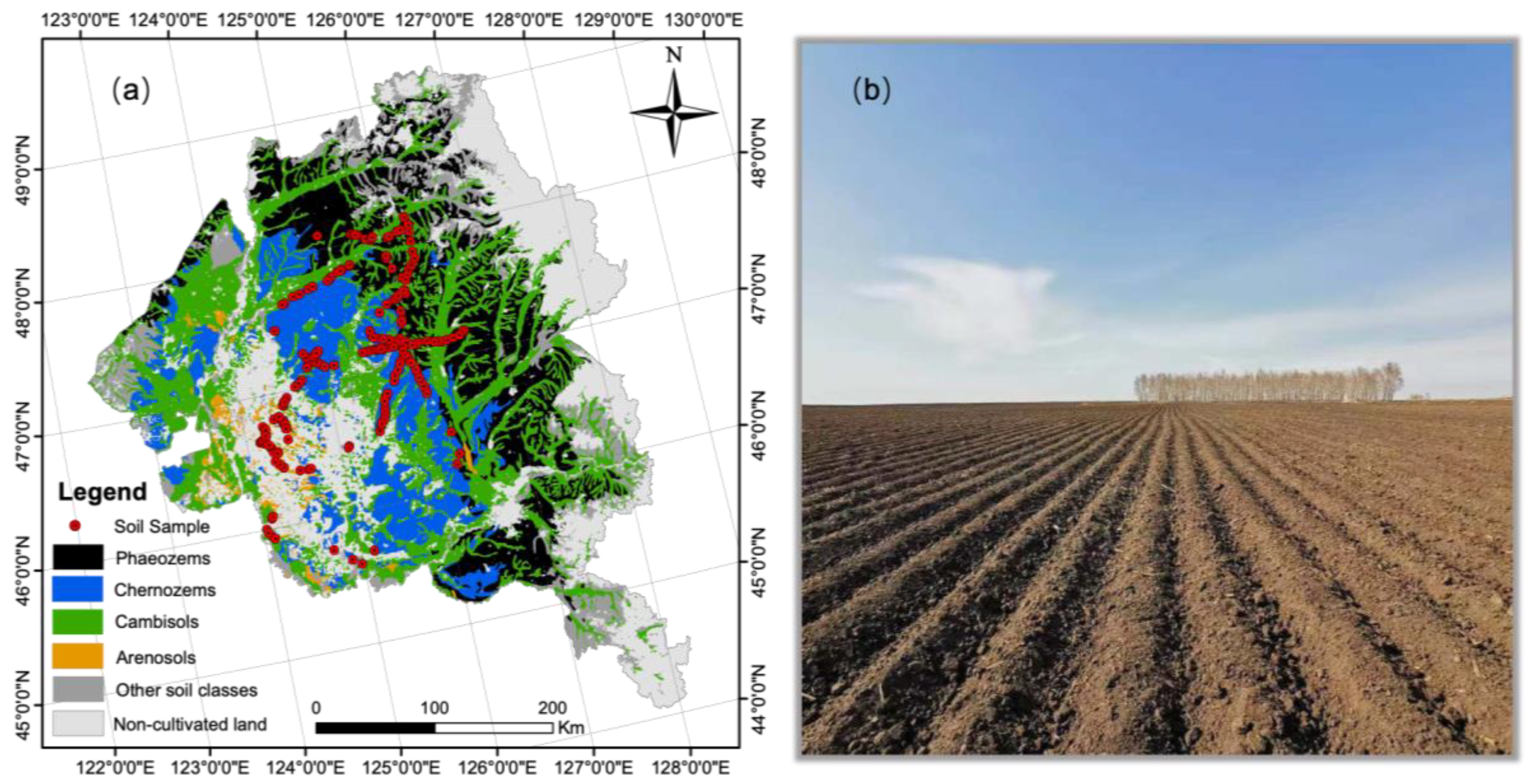
2.1. Study Area and Field Sampling

Our study area was located on the northern Songnen Plain (122~131°E, 43~49°N) (Figure 2). This area is an important food production base, with good natural conditions for crop growth. The climatic conditions are dominated by a temperate continental semi-arid and semi-humid monsoon climate, with an annual mean precipitation varying between 400 mm and 600 mm [68] and an annual average air temperature of 3.3 °C [69]. The overall terrain of the cultivated land in our study area is relatively flat. The elevation is high in the northeast and low in the southwest, ranging from 104~496 m. The study area has fertile soil resources with relatively high SOM contents; they provide good soil fertility conditions for planting various crops, such as maize, soybeans, and rice.
The Songnen Plain is commonly deemed to be an area with typical Mollisols [70,71]. Four soil types are mainly distributed in the cultivated land, including black soil, chernozems soil, aeolian soil, and meadow soil, which are represented as Phaeozems, Chernozems, Arenosols, and Cambisols in the World Reference Base for Soil Resources (WRB) [72,73]. Phaeozems and Chernozem are distributed in the northeastern part of Songnen Plain, and their SOM contents are higher than those of other soils. Arenosols are located in the southwest with low SOM content, and Cambisols are scattered among the other three soil types and distributed in low-lying areas.
Since the cultivated land in the study area is ploughed from the end of March to the beginning of April every year, the soil is exposed to the ground from then on. There is no snow cover or straw burning, almost no residual on the soil surface, and no large area of vegetation cover in the study area (Figure 2b), so from early April to late May belongs to the bare period of cultivated land, which is defined as the bare soil period. A field survey was conducted over the bare soil period to select the sample collection areas on the cultivated land of the Songnen Plain. The topsoil (0–20 cm) samples along the vertical profile of the soil were collected. To ensure that the SOM content of the sampling points would be representative, we selected flat and open cultivated lands along both sides of the highway for sample collection, and the sample intervals were about 10 km. We superimposed a 30 m spatial resolution digital ‘cultivated land’ mask on the soil map with ArcMap 10.2 to help select soil sampling locations. Then, 5–6 subsampling points were randomly selected in a square grid within a 30 × 30 m area. The soil samples were obtained by mixing the subsamples so that the measured SOM content can effectively reflect the average level of regional SOM content. Finally, a portable global positioning system (GPS, G350, Beijing UniStrong Science and Technology Limited Company, Beijing, China) was applied to record the geographic locations and collection times of each sample. In total, 281 soil samples from cultivated land were collected. The samples were placed in polyethylene plastic bags and kept at 4 °C until they were transported to the laboratory for analysis. Subsequently, the soil samples were air-dried, and fallen leaves and stones were removed from the samples. The samples were then passed through a 0.20 mm mesh [74] and measured for their SOM content using the potassium dichromate volumetric method [75].

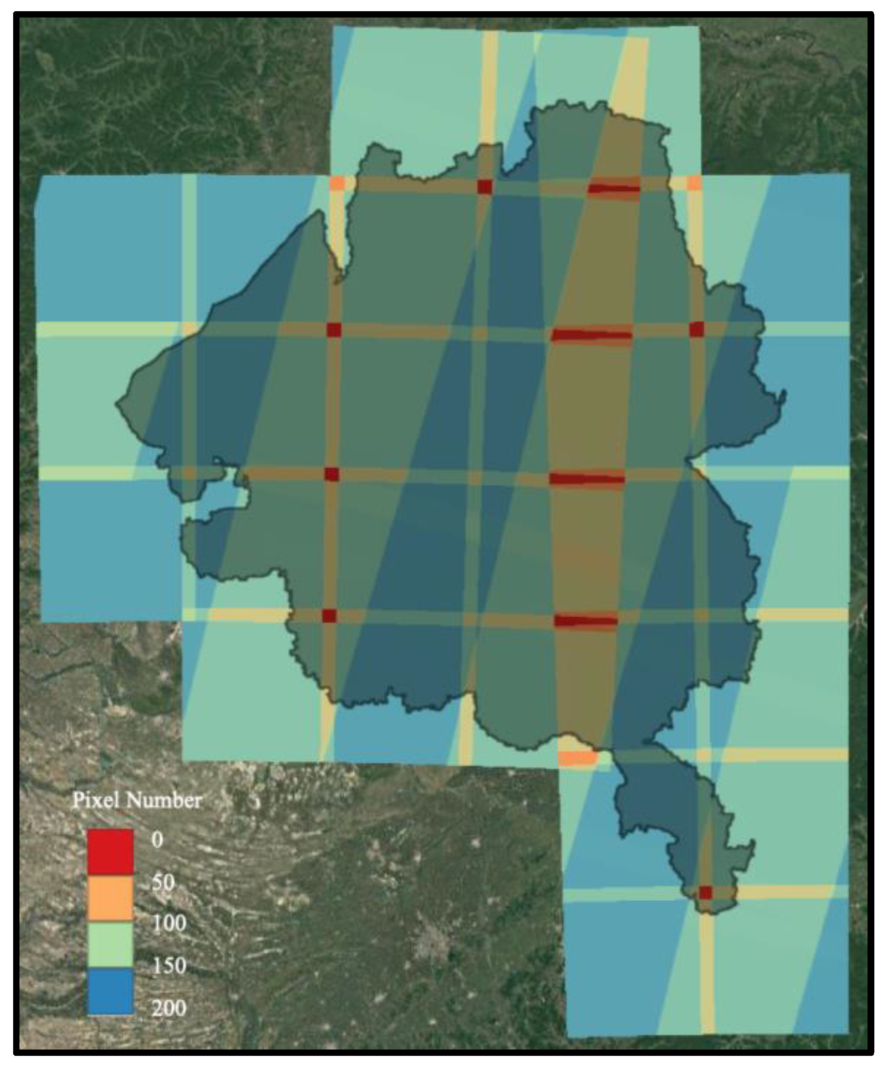
2.2. Remotely Sensed Imagery

2.2.1. Sentinel-2A and MODIS Satellite Data

Sentinel-2A and MOD09A1 images were used as the main remote sensing data for analysis and were derived from the GEE data pool (https://code.earthengine.google.com/, accessed on 28 June 2020). As the MOD09A1 image is a composite dataset, cloud processing is not required. For Sentinel-2A data, automatic cloud and cloud shadow masking methods were used, which creates gaps with no data in different locations for different image dates. After that, all available multi-temporal observations covering the study area were used to generate a seamless median composite imagery for the target year of 2020, which is conducive to reduce the poor observation effect caused by frequent clouds and shadows. In our study, remote sensing images in the bare soil period were used as data sources, which could effectively capture the surface information of bare cultivated soil and reduce interference, thereby obtaining a more real soil surface reflectance. In total, we used 1540 Sentinel-2A images and 14 MODIS images in the period of April to May in 2019–2020 (Figure 3). Table 1 shows the band parameter information for the Sentinel-2A and MOD09A1 imagery. The common bands for the Sentinel-2A and MOD09A1 images were b2 or b3 (blue band), b3 or b4 (green band), b4 or b1 (red band), b8 or b2 (NIR band), b11 or b6 (SWIR-1 band), and b12 or b7 (SWIR-2 band).

2.2.2. Land Cover Dataset

The MODIS land cover type product (MCD12Q1) was applied to obtain the land cover map of the Songnen Plain in 2020 at a 500 m spatial resolution [76]. It included 11 natural vegetation classes, three non-vegetated land classes, and three other classes that were obtained [77] using supervised classification and post-processing that incorporated prior knowledge to further refine specific classes. Therefore, the MCD12Q1 land cover type product was used to identify cropland pixels and extract the boundary of the croplands on the Songnen Plain for SOM prediction.

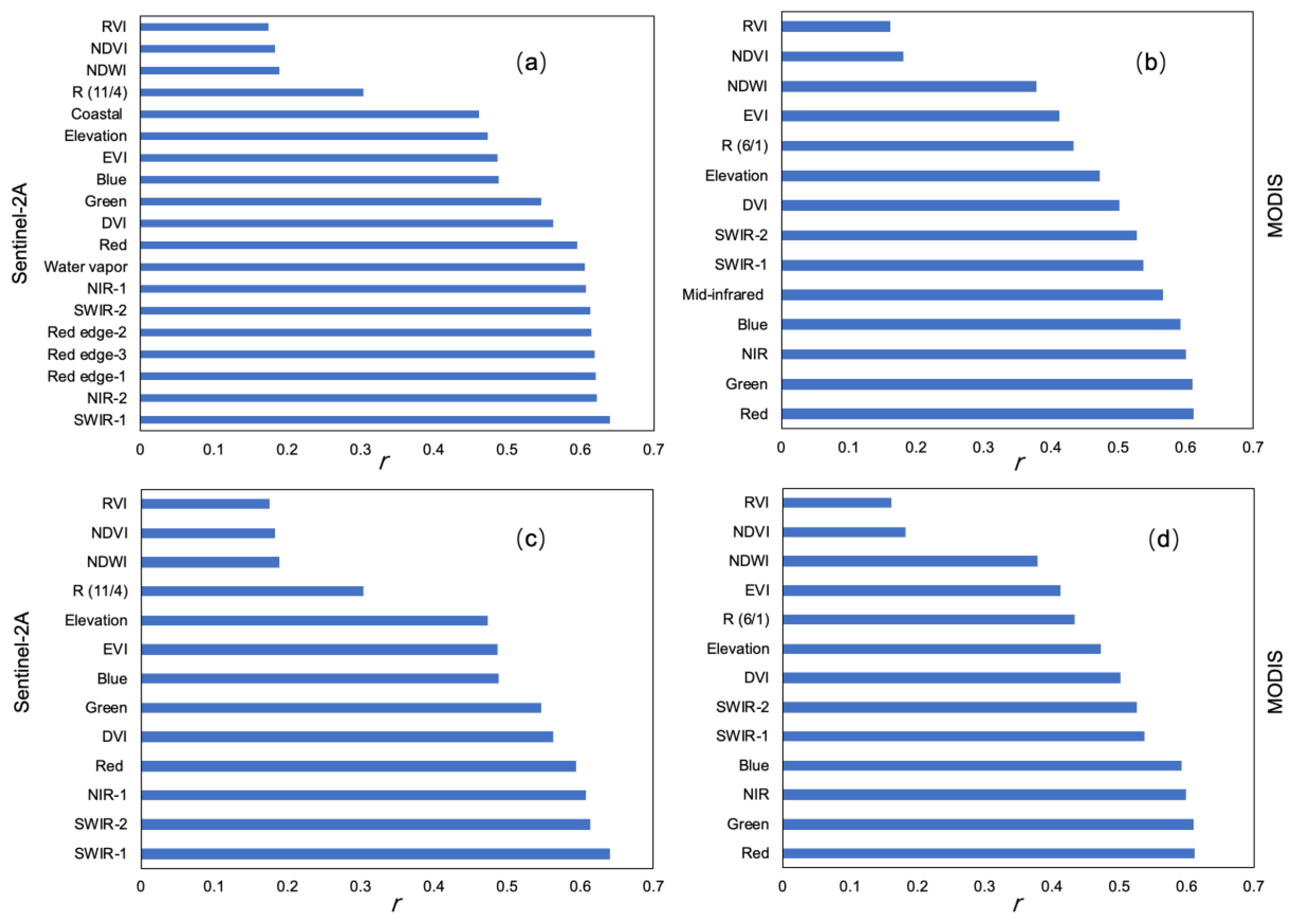
2.3. Variable Datasets Construction

Our variable dataset consisted of spectral bands, spectral indices, and terrain factor in this study. The scheme of full-band and common-band variable datasets using Sentinel-2A and MODIS images is shown in Table 2. The spectral bands were provided by Sentinel-2A and MODIS images. The calculations and descriptions of spectral indices and terrain factor are as follows.

2.3.1. Spectral Index Construction

A spectral index is an effective and rapid way to construct model input variables [78]. This approach can also reduce reflection spectrum errors and thereby improve the accuracy of SOM prediction [79,80]. We calculated the following indices: ratio spectral indices, such as R 11 ( 6 ) / 4 ( 1 ) [53,54,56], the ratio vegetation index (RVI) [50], and the enhanced vegetation index (EVI) [50,81,82]; difference spectral indices, such as the difference vegetation index (DVI) [50,83]; and normalized difference spectral indices, such as the normalized difference water index (NDWI) [50,84,85,86] and the normalized difference vegetation index (NDVI) [50,87,88]. Prior studies have proven that the ratio index, difference index, and normalized difference index are conducive to predicting SOM [54,58,89]. The typical moisture absorption bands in the soil spectrum at 1400, 1900, and 2200 nm [90] correspond to b11 (6) and b12 (7) of Sentinel-2A and MODIS imageries. According to previous SOM predictions in the literature covering the Songnen Plain over the bare period [53,54,56], R(6/1) was determined as the ratio of b6 to b1 based on MODIS imagery, which generally showed a good relationship with SOM and was thus used as the model input variable. This spectral index can denote soil moisture information and reduce the negative impact of precipitation on SOM prediction; thereby improving the prediction accuracy. Therefore,   R 11 ( 6 ) / 4 ( 1 ) was adopted as an empirical spectral index based on Sentinel-2A (i.e., R(11/4)) and MODIS (i.e., R(6/1)) images in our study. NDVI, EVI, RVI, and DVI are the four most commonly used vegetation spectral indices to characterize vegetation information, which are able to reduce the influence of early growing seedlings on SOM prediction and provide a better environment for SOM spatial prediction. Moreover, NDWI was constructed mainly reflecting the soil moisture status [91] when there was almost no crop coverage. The spectral indices listed above were calculated based on the following equations:
R 11 ( 6 ) / 4 ( 1 ) = b 11 ( 6 ) b 4 ( 1 )
R V I = b N I R 1 b r e d
EVI = 2.5 × b N I R 1 b r e d b N I R 1 + 6 b r e d 7.5 b b l u e + 1
D V I = b N I R 1 b r e d
N D V I = b N I R 1 b r e d b N I R 1 + b r e d
N D W I = b N I R 1 b S W I R 1 b N I R 1 + b S W I R 1
where b11 and b6 represent the Sentinel-2A and MODIS imagery SWIR-1 bands, respectively, and b4 and b1 represent the red bands of those two images.

2.3.2. Terrain Factor
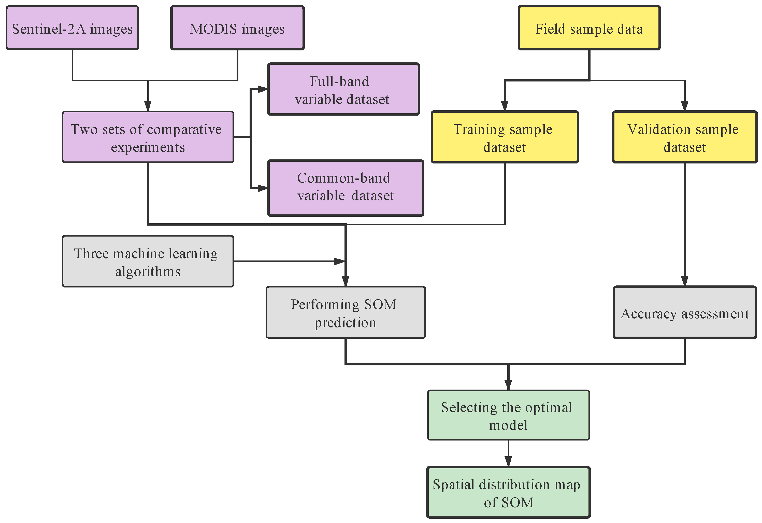
Elevation data was extracted from the World Wildlife Fund (WWF) HydroSHEDS void-filled DEM dataset; this dataset characterizes changes in soil’s physical and chemical properties at a spatial resolution of 90 m and was used for terrain analysis in this study. The elevation is a vital factor affecting the distribution of SOM for areas with relatively large terrain changes, which has been widely applied for producing land cover maps [92,93,94,95] and performing soil attribute predictions [50,66].

2.4. Methodology

2.4.1. Machine Learning Algorithms

RF is an ensemble decision tree (DT)-based machine learning algorithm, and the predicted SOM content was determined by the results of multiple DTs [96,97]. The RF algorithm uses mainly the bootstrap aggregating technique (bagging) and the recursive partitioning method to combine and average the prediction results of multiple unrelated DTs [98]. It performs SOM prediction by using a feedback iteration process and calculates the out-of-bag (OOB) error [97] to achieve the optimal prediction result, thereby avoiding model variability and instability [20,99]. We applied the random forest function [100] on the GEE cloud platform to perform SOM prediction. Here, three parameters were required to establish the RF models: the number of trees (i.e., n-tree), many features in each split (i.e., m-try), and the minimum number of samples that needed to occur on a leaf node (i.e., min_samples_leaf); these values were set to 300, 3, and 5, respectively.
SVR is a form of support vector machine (SVM) that aims to solve regression problems based on the support vector concept. Due to the high applicability and robustness of the model constructed by the SVM algorithm, it has been widely used in classification and regression problems in various fields [58,101,102]. Notably, setting the kernel function and the parameter C is extremely important for obtaining good model performance [58]. The kernel function is applied to project the dataset into a high-dimensional feature space and then to perform the regression prediction process. Meanwhile, the optimal parameter C value was determined by the minimum root mean squared error (RMSE) [58]. We used the kernlab package in R software [47] and the radial basis function (RBF) as the kernel function for performing SOM predictions in our study.
A back-propagation ANN was applied in our study that constructed a non-linear, non-parametric estimation error back-propagation regression model [103]. The input layer includes the independent variables used to perform the predictions and continuously feeds back the learning results (i.e., the bias) to the hidden layer. Then, the hidden layer discerns the complexity of the prediction model and implements non-linear mapping [40]. Finally, the output layer obtains a trained neural network. Through the process of forward and backward propagation, a trained model can calculate the gradient, update the weight of the network, and estimate the biases; that is, the biases are continuously assigned to each layer of the “neuron” until the biases of the neural network reach an acceptable range, thus stopping the running program and achieving the regression prediction of SOM [40,58]. The ANN model was constructed by programming it in MATLAB software, and the optimal prediction accuracy was evaluated on the basis of the RMSE value.

2.4.2. Assessment and Prediction

To assess the model accuracy, the soil sample data were randomly divided into two groups: 75% [46] of the sample data was used to train the models, and the remaining 25% was used for validation purposes. The RMSE [50,104,105,106] and the coefficient of determination (R2) [104,107] were used to evaluate the prediction accuracy of the models. The mean error (ME) [11,19,20,50] was applied to assess the unbiased prediction. Furthermore, we also used relative improvement (RI) in the RMSE [52,108] to measure the improvement in the prediction accuracy achieved by using the Sentinel-2A dataset rather than the MODIS dataset. These statistical indicators were calculated with the following equations:
RMSE = i = 1 n ( o i p i ) 2 n
R 2 = 1 i = 1 n ( p i o i ) 2 i = 1 n ( o i o ¯ ) 2
M E = 1 n i = 1 n ( o i p i )
R I = R M S E m R M S E n R M S E m × 100 %
where oi and pi denote the observed and predicted SOM values, respectively; n denotes the number of soil samples used for validation; p ¯ and o ¯ denote the means of the predicted and observed SOM values; and R M S E m and R M S E n denote the RMSE values for a single machine learning algorithm model using MODIS and Sentinel-2A imagery, respectively.
Identifying the optimal model based on the accuracy of the SOM prediction results was crucial for mapping the spatial distribution of SOM content with sufficient accuracy. The optimal model generally has a lower RMSE value and higher R2 value, denoting higher prediction accuracy [40,54], with the RMSE value approaching 0 and R2 value approaching 1 [20,40]. The ME value approaching zero signifies an unbiased prediction [20]. Therefore, in this study, the optimal model was identified and used to produce the spatial distribution map of SOM content.

3. Results and Analysis

3.1. Descriptive Statistics of the SOM Content

The descriptive statistics for the SOM contents in the whole, training, and validation datasets were performed with SPSS Statistics 22 software and are shown in Table 3. The measured SOM content in the whole soil sampling dataset ranged from 0.43 to 7.90%, with a mean of 3.85% and a standard deviation (SD) of 1.21. The measured SOM contents in the whole, training, and validation datasets had similar mean and SD values, indicating that the soil samples in the randomly allocated training and validation datasets had high representativeness. Therefore, the prediction results could reflect the spatial distribution patterns of SOM with sufficient accuracy.

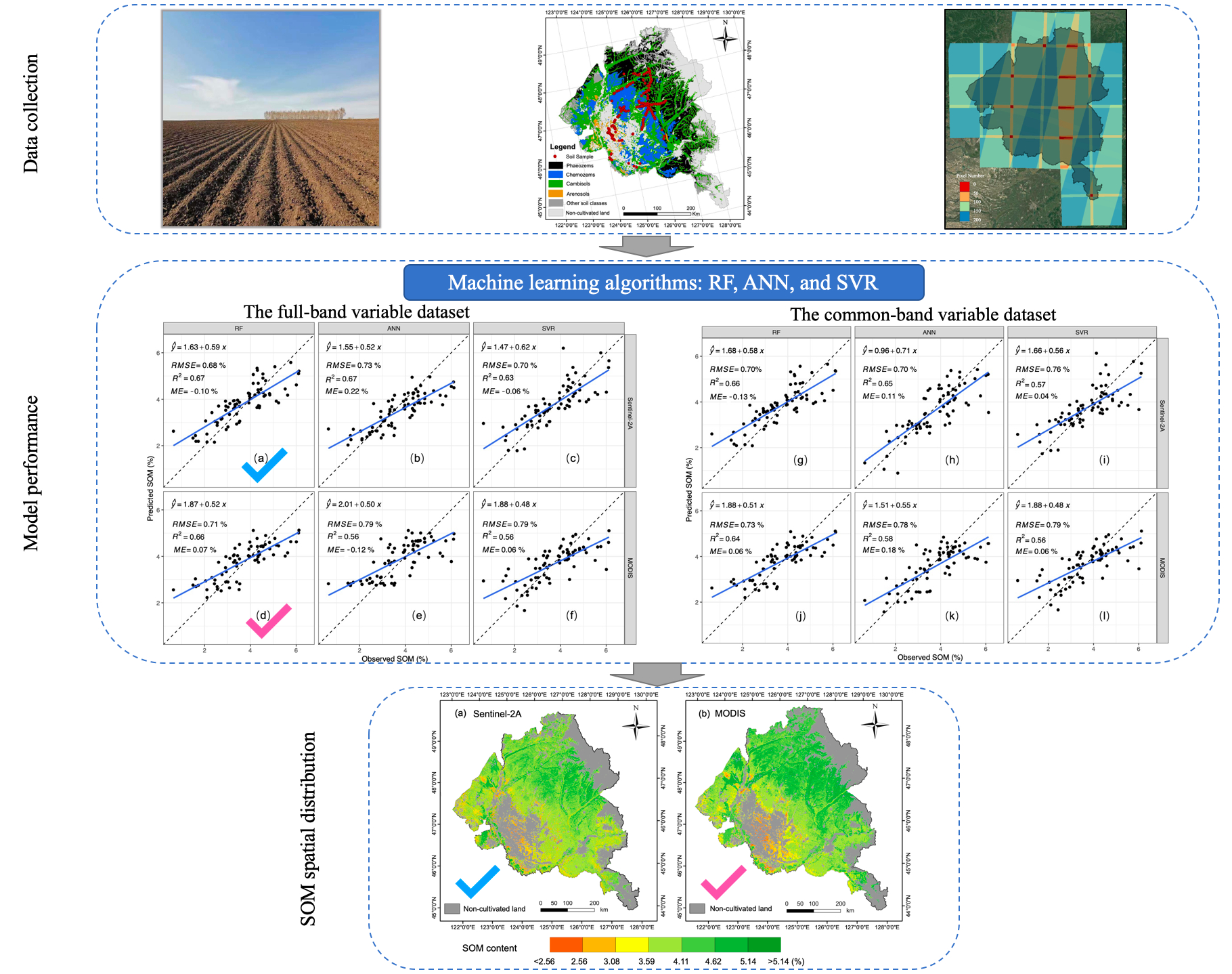
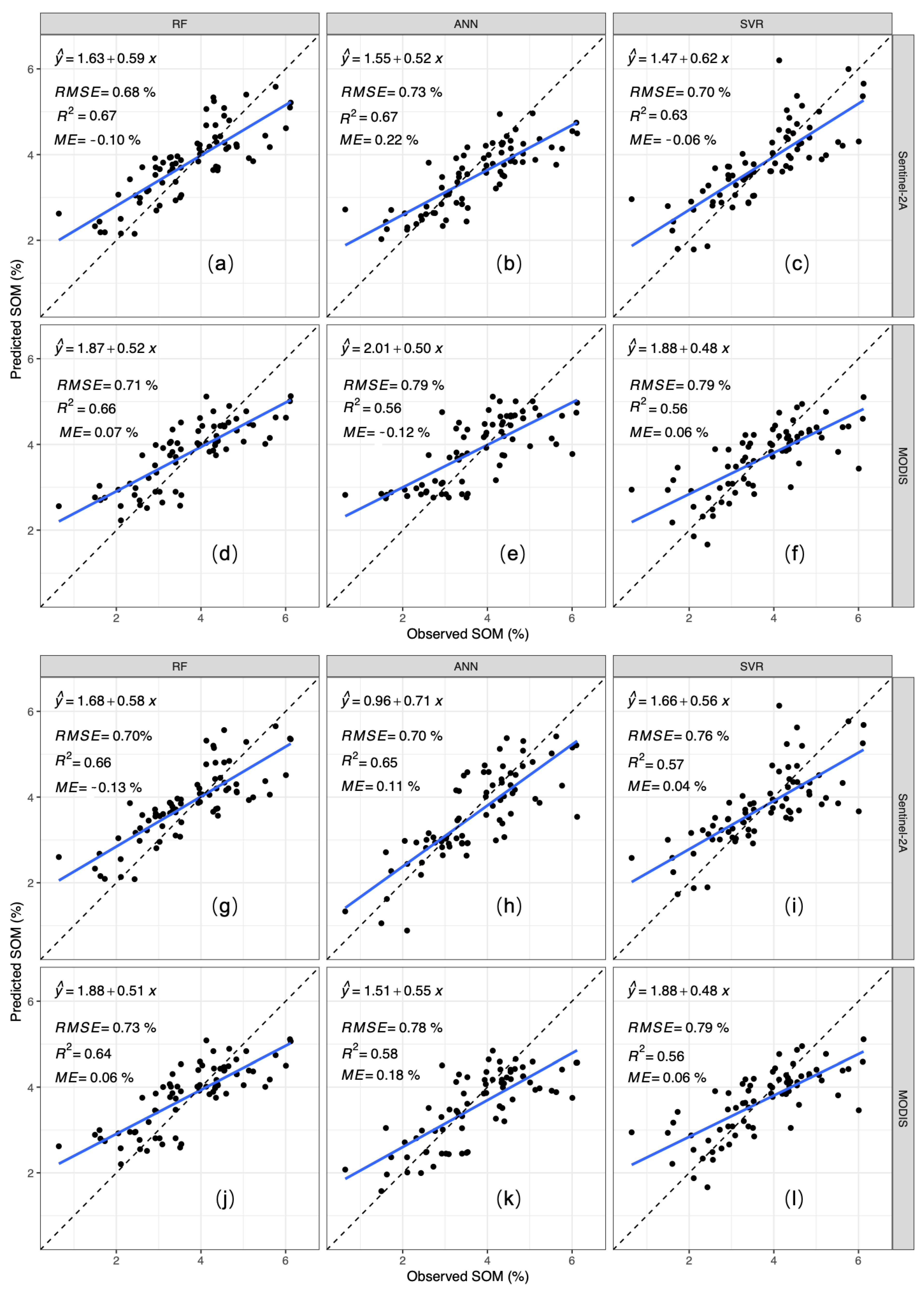
3.2. Model Performance

The Pearson correlation coefficients (r) between the independent variable and the SOM content were calculated and then used to rank all the independent variables. Figure 4 shows the correlation analysis results based on the full-band (Figure 4a,b) and common-band (Figure 4c,d) variable datasets of the Sentinel-2A and MODIS images. We found that the independent variables as the model inputs had a good correlation coefficient with the SOM content on all of the predicted scenarios. The level of statistical significance of the variables was p < 0.01.
Figure 5 shows the performances of the RF, ANN, and SVR models in predicting SOM based on the full-band (Figure 5a–f) and common-band (Figure 5g–l) variable datasets from the Sentinel-2A and MODIS images. In two sets of comparative experiments, we found that the model performances of the three machine learning algorithms based on Sentinel-2A images were better than those of the algorithms based on the MODIS images. As shown in Figure 5a–f, the RF, ANN, and SVR models had lower RMSE values (0.68%, 0.73%, and 0.70%) and higher R2 (0.67, 0.67, and 0.63) values when they were based on the Sentinel-2A dataset (Figure 5a–c); in contrast, the three models had slightly higher RMSE values (0.71%, 0.79%, and 0.79%) and lower R2 values (0.66, 0.56, and 0.56) when they were based on the MODIS dataset (Figure 5d–f). Notably, these results also demonstrate that the multi-band characteristics of Sentinel-2A images make them more helpful than MODIS images for predicting SOM with high accuracy. Simultaneously, the ME values were overall low. The lower ME values were generally obtained by SVR and RF algorithms and the highest was obtained by ANN algorithm on all of the predicted scenarios. Moreover, comparing Figure 5g–i and Figure 5j–l when the common-band variable datasets of Sentinel-2A and MODIS images were used as model inputs, the model performances of the three machine learning algorithms of the former (Figure 5g–i) achieved lower RMSE values (0.70%, 0.70%, and 0.76%) and higher R2 (0.66, 0.65, and 0.57) values, whereas, the latter (Figure 5j–l) achieved higher RMSE values (0.73%, 0.78%, and 0.79%) and lower R2 values (0.64, 0.58, and 0.56), which is due to the high spatial resolution of the Sentinel-2A images resulting in improved prediction accuracy.
Comparing the statistical indicator of RMSE values, the application of Sentinel-2A data resulted in mean RIs of 7.67% and 5.87% compared to the application of MODIS data, respectively, in the two sets of comparative experiments. Moreover, the above results also indicated that the predictive ability of the RF models produced a lower RMSE (0.68%) and a higher R2 (0.67) in all of the predicted scenarios than those of the ANN and SVR models; therefore, the RF model achieved the highest prediction accuracy when it was based on the variable datasets from the full-band Sentinel-2A images, and was selected as the optimal prediction model.
In addition, we also mapped the spatial distribution of the residuals (Figure 6) of the optimal prediction model. The values of residuals were divided into six levels and given different colours so that the spatial distribution characteristics of the values of each level can be clearly observed. Figure 6 showed that the residual points of different levels were irregular and randomly distributed without a clustered distribution that is too high or too low in a certain area. Therefore, the SOM prediction model established in our study is suitable for performing SOM prediction, which can be used to draw the spatial distribution map of SOM in the Songnen Plain.

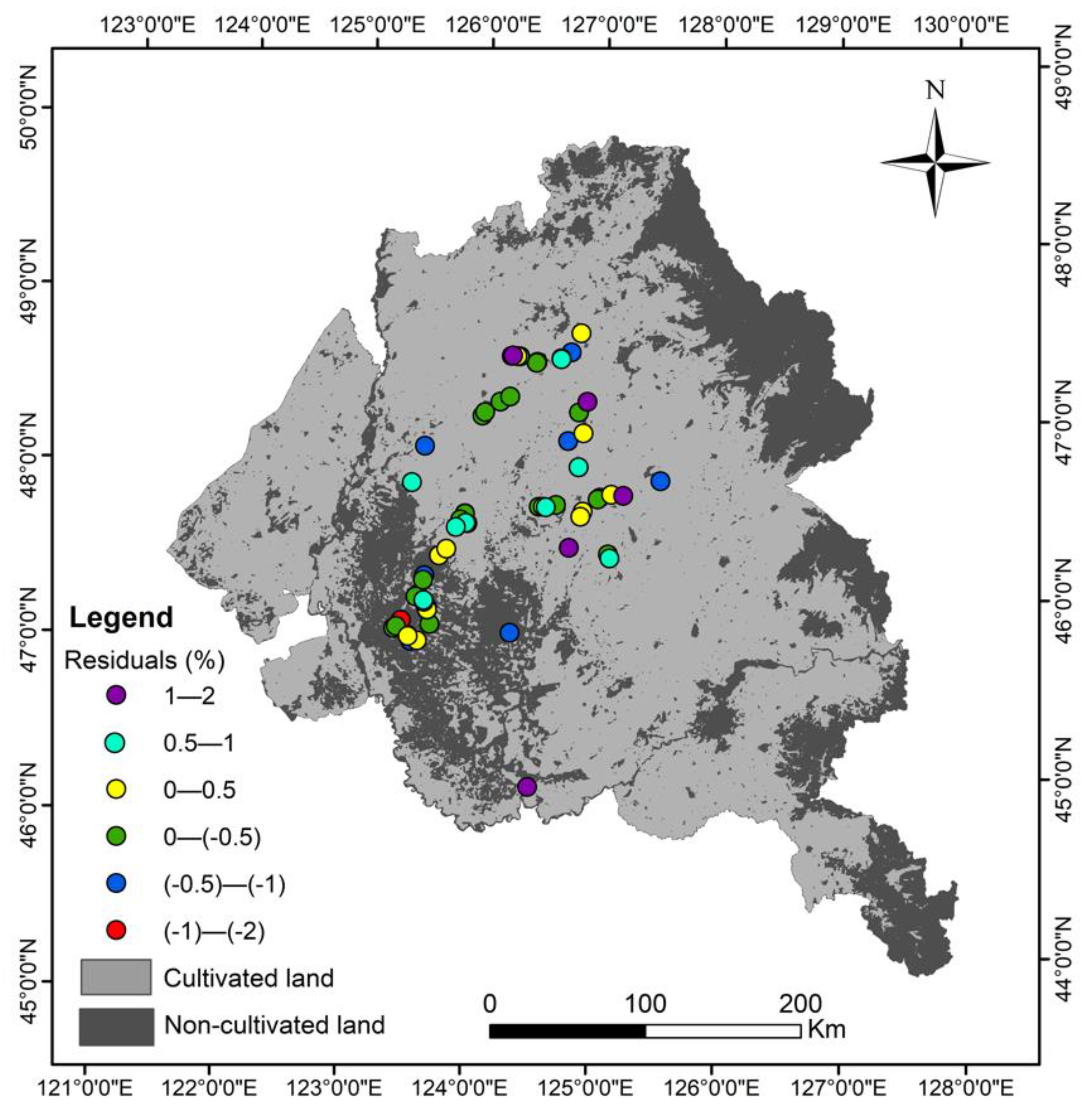
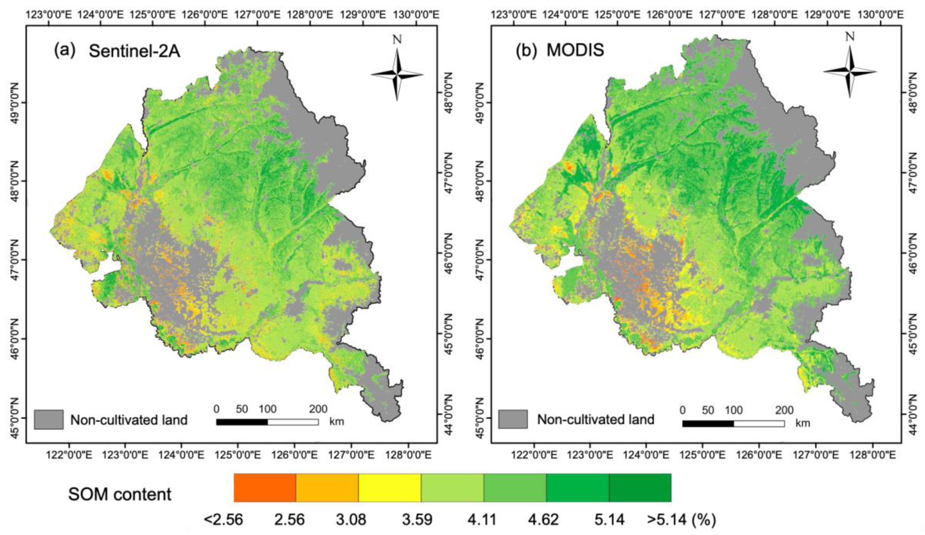
3.3. Spatial Characteristics of Predicted SOM Map

To demonstrate the result of the optimal prediction in our experiment and implement a comparative analysis of the mapping results of the two images, the SOM content of the study area was mapped based on the predictions generated from full-band Sentinel-2A (Figure 7a) and MODIS (Figure 7b) imagery datasets by the RF algorithm (Figure 7). Figure 7a,b both showed that the SOM content was predicted to be high in the northeastern part of the study area and low in the southwestern part, which is consistent with the literature [53,54,56,58,59]. Due to the high latitude, cold environment, and distribution of SOM-rich soil types (e.g., Phaeozems and Chernozems) in the northeastern part of the study area, the predicted SOM was higher in this region. However, low-SOM soil types (e.g., Arenosols) and pastoral areas are widely distributed in the southwestern part of the study area, and the predicted SOM in that region was relatively low. Since Cambisols are usually distributed in low-lying areas, the migration of soil caused by external conditions such as rainwater led to the soil accumulating in these areas, resulting in a higher SOM content. Therefore, the SOM content on the Songnen Plain generally exhibited a trend of being high in the northeast and low in the southwest.

4. Discussion

4.1. Comparison of Sentinel-2A-Based and MODIS-Based Models

SOM prediction methods using satellite remote sensing data have made considerable progress. Numerous studies have applied satellite remote sensing data, including moderate-resolution data such as MODIS images, to perform SOM prediction and map its spatial distribution patterns [30,50,54,66,77,109]. However, the use of MODIS products (e.g., MOD09A1) has some limitations. First, each MOD09A1 image is an eight-day composite dataset, and the temporal information associated with each pixel may be inconsistent [54]; this can increase the negative effects of the spatial heterogeneity of soil properties and the spatial variations in pixel temporal information and soil moisture, resulting in lower prediction accuracy. Second, the accuracy of SOM prediction models can be influenced by the satellite image quality and environmental factors, and the pixels in MODIS images may reflect abnormal conditions in local areas. This is especially notable in MOD09A1 images with a 500 m resolution and may lead to anomalies in soil surface reflectivity that reduce the accuracy of SOM prediction. Therefore, the prediction accuracy of models based on MODIS data is limited due to the high subpixel heterogeneity [110,111].
We established two sets of comparative experiments and constructed separate full-band and common-band variable datasets, which aimed at comparing the performances of Sentinel-2A and MODIS data from the perspectives of spectral information richness and spatial resolution. The results demonstrated that the accuracies of the three machine learning algorithms that used Sentinel-2A data were all higher than those of the algorithms that used MODIS data because of the richer spectral information contained in the multi-band series and the higher spatial resolution of the Sentinel-2A data. The superiority of Sentinel-2 images has also been verified in other research fields [111,112]. Therefore, our study suggests that using Sentinel-2A images can significantly improve SOM prediction accuracy and may provide opportunities to generate high-resolution, high-precision maps of the spatial distribution of SOM.

4.2. Applicability of Machine Learning Algorithms

The results showed that the RF algorithm achieved slightly better performance than the ANN and SVR algorithms. Consistent with the existing literature, the RF algorithm represented a promising approach for mapping the spatial patterns of SOM at the regional scale. For example, Mahmoudzadeh et al. [113] applied RF, which outperformed the SVM and cubist (CU) algorithms, to predict the spatial distribution of SOM in western Iran. Tziachris et al. [20] confirmed that the RF algorithm consistently outperformed the regression kriging (RK) algorithm for soil attribute mapping. Moreover, Chen et al. [50] demonstrated that compared to DT and bagging DT (BDT) algorithms, the RF attained a higher R2 value when evaluating the SOM changes at the regional scale. Simultaneously, our study achieved better model performance based on Sentinel-2A images using the RF algorithm compared to the previous research result in the Songnen Plain. Dou et al. [54] established a regional SOM prediction model and mapped the spatial distribution of SOM content using the stepwise multiple regression method based on MODIS images, but the RMSE value (0.81%) was higher than that of our study (0.68%). Therefore, the RF algorithm has been widely recognized in SOM prediction at the regional scale and yielded promising model performance.
The use of the RF algorithm provided certain advantages that can be summarized as: (1) RFs can not only quickly predict the training and validation datasets but can also effectively avoid overfitting due to the implementation of random sampling strategies [44,58]; (2) the multicollinearity problem between features can be effectively avoided, supporting high-dimensional features [114,115]; (3) the hierarchical relationships can be characterized, showing good stability in regard to missing and unbalanced data [116]; (4) it has strong robustness to the outliers in the variables, and handles these outliers through the binding method [117]; (5) they can also provide the importance of explanatory variables to determine their contributions for the model and the main predictive factors [117,118]. Moreover, the RF algorithm also has significant advantages in terms of OOB error, and it is generally considered a good estimate of the expected error of unseen data [119]. Although machine learning algorithms can handle non-linear and missing data well and can effectively avoid multicollinearity between features, SVR and back-propagation ANNs have certain limitations. For instance, the back-propagation ANN algorithm is similar to a “black box” [58,120,121]; it is difficult to find the appropriate kernel function for the SVM for each specific application, and the algorithm is highly complex [122,123,124]. Simultaneously, due to the spatial variability in climatic conditions, soil parent materials, human activities, and land use management, the prediction accuracy of different algorithm models may vary greatly among different study areas, and no single algorithm is universally applicable for different regions [50,51]. Therefore, future studies should consider how to obtain a more universal SOM prediction model and improve the computational efficiency of such a model to enhance its practical applicability.

4.3. Advantages of the Google Earth Engine for SOM Prediction

As a comprehensive big data platform for resource integration, GEE is a cloud-based geospatial analysis platform that provides large storage and robust computing capacities [92,125]. It allows users to easily access interactive remote sensing images and algorithms to perform scientific analyses for research and visualize geographic system information [126]. Currently, the GEE data pool includes a catalogue of satellite images and geospatial datasets from numerous remote sensing satellites around the world that spans more than 40 years [92,125]. Although GEE has been widely applied for the production of land cover type maps [92,93,94,95], it is rarely used in studies of the spatial prediction of soil properties. Thus, the application of GEE for SOM prediction requires further exploration and development. In our study, the GEE cloud platform was applied to allow rapid access and complex pre-processing of time series Sentinel-2A and MODIS images without requiring local downloads. In addition, the RF algorithm was used with the algorithm function of the GEE platform to generate a high-precision spatial distribution map of SOM. Therefore, the usage of GEE can greatly improve the efficiency of scientific researchers [127], and it has been widely applied in scientific research in many fields at local, regional, and global scales [92,125].

4.4. Limitations and Future Researches

We identified three limitations to this study. First, we chose to predict SOM with only Sentinel-2A and MODIS imagery datasets, and the bare soil period for cultivated land was adopted as our research period. Due to the limitation of the short bare period and the influence of clouds, few images covering the study area can be effectively used, so the time-series images were applied to generate seamless composite images in our study. The composite image can make up for the lack of single image information caused by the poor observation effect with frequent clouds reduce the impact of different ground conditions, and eliminate vegetation information [128]. However, only a few studies have applied composite images to predict SOM [50] or soil organic carbon (SOC) [129,130,131], which is because the application potential and interpretability of these composite images need to be further evaluated.Therefore, future studies should attempt to assess other remote sensing image sources with high spatial-temporal resolution [58,107,132,133,134] and fusion images of different time periods or types [135,136] to decrease the uncertainty in SOM predictions at the regional scale, thereby achieving more accurate maps of the spatial distribution of SOM. Secondly, our results demonstrated that the RF algorithm resulted in better model performance than the ANN and SVR algorithms. Nevertheless, other methods should also be tested to achieve better model performance for SOM prediction in future studies. Potential methods include Bayesian maximum entropy (BME) [82], geographically weighted RK (GWRK) [137,138] and hybrid algorithms (e.g., ANN-kriging, RF-kriging) [20,139], which have been applied for SOM prediction. It has also been shown that integrating different algorithms or images generally improves the accuracy of SOM mapping at the regional scale.
Furthermore, the prediction accuracies achieved in our study were considered satisfactory, but a good model should exhibit not only excellent performance but also strong robustness and generalization ability [40]. It has been widely recognized that the use of spatially related auxiliary variables can effectively improve the prediction accuracy of soil attributes, and the spatial distribution pattern of SOM are generally controlled by environmental variables such as elevation [55,140]. Our results showed that elevation had a higher correlation with SOM, and was adopted as the model input variable. Consistent with previous research, elevation is an important topographical attribute and as the model input variable to investigate the impact of terrain conditions on SOM content levels [20,30,40,50,141]. However, the SOM distribution is controlled by multiple environmental factors, such as climatic condition, geological units, vegetation cover information, and land use measures [19,23,139,142]. Therefore, the objective of future research is to build a more comprehensive and appropriate set of feature variables and to incorporate various specific agricultural management practices in order to improve the accuracy of SOM prediction and more accurately map the spatial distribution of SOM.

5. Conclusions

Using the GEE cloud platform, we built separate full-band and common-band variable datasets with Sentinel-2A and MODIS datasets in order to confirm the superiority of the Sentinel-2A dataset. We also evaluated the performances of the RF, ANN, and SVR algorithms for SOM prediction and finally generated the spatial distribution map of SOM across the croplands on the Songnen Plain. Our findings indicated that the prediction results of the model based on Sentinel-2A data showed a good relationship with the actual SOM data, thereby Sentinel-2A data achieved better results than MODIS data for SOM mapping on the Songnen Plain due to the higher spectral and spatial resolutions. Moreover, the RF model generally performed better than the ANN and SVR models. The GEE cloud platform provided an ideal and rapid way to obtain various time series remote sensing image data and to implement SOM prediction using a machine learning algorithm function. As expected, the SOM content was higher on the northeastern and lower on the southwestern Songnen Plain. This study provides promising insights into SOM mapping and a data reference for assessing soil carbon pools.

Author Contributions

Conceptualization, M.Z. (Meiwei Zhang) and H.L.; methodology, M.Z. (Meiwei Zhang) and M.Z. (Meinan Zhang); software, M.Z. (Meiwei Zhang) and M.Z. (Meinan Zhang); validation, M.Z. (Meiwei Zhang).; investigation, M.Z. (Meiwei Zhang) and H.L.; writing—original draft preparation, M.Z. (Meiwei Zhang); writing—review and editing, M.Z. (Meinan Zhang), H.Y., Y.J., H.L., and X.Z.; visualization, M.Z. (Meiwei Zhang) and M.Z. (Meinan Zhang); supervision, H.L.; funding acquisition, H.L. All authors have read and agreed to the published version of the manuscript.

Funding

This research was funded by the K.C. Wong Education Foundation and the “Academic Backbone” Project of Northeast Agricultural University.

Institutional Review Board Statement

Not applicable.

Informed Consent Statement

Not applicable.

Data Availability Statement

The data presented in this study are available on request from the corresponding author. The data are not publicly available due to privacy.

Acknowledgments

We would like to sincerely thank the editors and anonymous reviewers for their valuable and constructive suggestions that helped us improve the manuscript.

Conflicts of Interest

The authors declare no conflict of interest.

References

  1. Sparling, G.P.; Wheeler, D.; Vesely, E.-T.; Schipper, L.A. What is Soil Organic Matter Worth? J. Environ. Qual. 2006, 35, 548–557. [Google Scholar] [CrossRef]
  2. Zhang, L.; Liu, Y.; Li, X.; Huang, L.; Yu, D.; Shi, X.; Chen, H.; Xing, S. Effects of soil map scales on simulating soil organic carbon changes of upland soils in Eastern China. Geoderma 2018, 312, 159–169. [Google Scholar] [CrossRef]
  3. Manlay, R.J.; Feller, C.; Swift, M. Historical evolution of soil organic matter concepts and their relationships with the fertility and sustainability of cropping systems. Agric. Ecosyst. Environ. 2007, 119, 217–233. [Google Scholar] [CrossRef]
  4. Liang, Z.; Chen, S.; Yang, Y.; Zhao, R.; Shi, Z.; Rossel, R.A.V. National digital soil map of organic matter in topsoil and its associated uncertainty in 1980’s China. Geoderma 2019, 335, 47–56. [Google Scholar] [CrossRef]
  5. Guo, L.; Zhao, C.; Zhang, H.; Chen, Y.; Linderman, M.; Zhang, Q.; Liu, Y. Comparisons of spatial and non-spatial models for predicting soil carbon content based on visible and near-infrared spectral technology. Geoderma 2017, 285, 280–292. [Google Scholar] [CrossRef]
  6. Huang, B.; Sun, W.; Zhao, Y.; Zhu, J.; Yang, R.; Zou, Z.; Ding, F.; Su, J. Temporal and spatial variability of soil organic matter and total nitrogen in an agricultural ecosystem as affected by farming practices. Geoderma 2007, 139, 336–345. [Google Scholar] [CrossRef]
  7. Nocita, M.; Stevens, A.; Noon, C.; van Wesemael, B. Prediction of soil organic carbon for different levels of soil moisture using Vis-NIR spectroscopy. Geoderma 2013, 199, 37–42. [Google Scholar] [CrossRef]
  8. Feng, N.; Hongfen, Z.; Rutian, B. Hyperspectral prediction of soil organic matter content in the Reclamation cropland of Coal Mining Areas in the Loess Platesu. Sci. Agric. Sin. 2016, 49, 2126–2135. [Google Scholar]
  9. Juice, S.M.; Templer, P.H.; Phillips, N.G.; Ellison, A.M.; Pelini, S.L. Ecosystem warming increases sap flow rates of northern red oak trees. Ecosphere 2016, 7, e01221. [Google Scholar] [CrossRef]
  10. Mishra, U.; Torn, M.S.; Masanet, E.; Ogle, S.M. Improving regional soil carbon inventories: Combining the IPCC carbon inventory method with regression kriging. Geoderma 2012, 189–190, 288–295. [Google Scholar] [CrossRef]
  11. Were, K.; Bui, D.T.; Dick, Ø.B.; Singh, B.R. A comparative assessment of support vector regression, artificial neural networks, and random forests for predicting and mapping soil organic carbon stocks across an Afromontane landscape. Ecol. Indic. 2015, 52, 394–403. [Google Scholar] [CrossRef]
  12. Meersmans, J.; De Ridder, F.; Canters, F.; De Baets, S.; Van Molle, M. A multiple regression approach to assess the spatial distribution of Soil Organic Carbon (SOC) at the regional scale (Flanders, Belgium). Geoderma 2008, 143, 1–13. [Google Scholar] [CrossRef]
  13. Walkley, A.; Black, I.A. An examination of the Degtjareff method for determining soil organic matter, and a proposed modification of the chromic acid titration method. Soil Sci. 1934, 37, 29–38. [Google Scholar] [CrossRef]
  14. Van Raij, B.; Andrade, J.C.; de Cantarella, H.; Quaggio, J.A. Análise Química para Avaliação da Fertilidade de Solos Tropicais; Instituto Agronômico: Campinas, Brazil, 2001.
  15. Lagacherie, P. Digital Soil Mapping: A State of the Art. Digit. Soil Mapp. Ltd. Data 2008, 3–14. [Google Scholar] [CrossRef]
  16. Bie, S.W.; Beckett, P.H.T. Quality control in soil survey: II. The costs of soil survey. J. Soil Sci. 1971, 22, 453–465. [Google Scholar] [CrossRef]
  17. Zhao, Z.; Ashraf, M.I.; Meng, F.-R. Model prediction of soil drainage classes over a large area using a limited number of field samples: A case study in the province of Nova Scotia, Canada. Can. J. Soil Sci. 2013, 93, 73–83. [Google Scholar] [CrossRef]
  18. Matheron, G. Principles of geostatistics. Econ. Geol. 1963, 58, 1246–1266. [Google Scholar] [CrossRef]
  19. Zhang, S.; Huang, Y.; Shen, C.; Ye, H.; Du, Y. Spatial prediction of soil organic matter using terrain indices and categorical variables as auxiliary information. Geoderma 2012, 171–172, 35–43. [Google Scholar] [CrossRef]
  20. Tziachris, P.; Aschonitis, V.; Chatzistathis, T.; Papadopoulou, M. Assessment of spatial hybrid methods for predicting soil organic matter using DEM derivatives and soil parameters. Catena 2019, 174, 206–216. [Google Scholar] [CrossRef]
  21. Schloeder, C.; Zimmerman, N.; Jacobs, M. Comparison of Methods for Interpolating Soil Properties Using Limited Data. Soil Sci. Soc. Am. J. 2001, 65, 470–479. [Google Scholar] [CrossRef]
  22. Wu, C.; Wu, J.; Luo, Y.; Zhang, L.; Degloria, S.D. Spatial Prediction of Soil Organic Matter Content Using Cokriging with Remotely Sensed Data. Soil Sci. Soc. Am. J. 2009, 73, 1202–1208. [Google Scholar] [CrossRef]
  23. Dai, F.; Zhou, Q.; Lv, Z.; Wang, X.; Liu, G. Spatial prediction of soil organic matter content integrating artificial neural network and ordinary kriging in Tibetan Plateau. Ecol. Indic. 2014, 45, 184–194. [Google Scholar] [CrossRef]
  24. Heuvelink, G.; Bierkens, M.F.P. Combining soil maps with interpolations from point observations to predict quantitative soil properties. Geoderma 1992, 55, 1–15. [Google Scholar] [CrossRef]
  25. McBratney, A.B.; Santos, M.M.; Minasny, B. On digital soil mapping. Geoderma 2003, 117, 3–52. [Google Scholar] [CrossRef]
  26. Zhao, Z.; Yang, Q.; Benoy, G.; Chow, T.L.; Xing, Z.; Rees, H.W.; Meng, F.-R. Using artificial neural network models to produce soil organic carbon content distribution maps across landscapes. Can. J. Soil Sci. 2010, 90, 75–87. [Google Scholar] [CrossRef]
  27. Ward, K.J.; Chabrillat, S.; Neumann, C.; Foerster, S. A remote sensing adapted approach for soil organic carbon prediction based on the spectrally clustered LUCAS soil database. Geoderma 2019, 353, 297–307. [Google Scholar] [CrossRef]
  28. Webster, R.; Oliver, M.A. Geostatistics for Environmental Scientists; John Wiley & Sons: Hoboken, NJ, USA, 2007. [Google Scholar]
  29. Guo, P.-T.; Wu, W.; Sheng, Q.-K.; Li, M.-F.; Liu, H.-B.; Wang, Z.-Y. Prediction of soil organic matter using artificial neural network and topographic indicators in hilly areas. Nutr. Cycl. Agroecosyst. 2013, 95, 333–344. [Google Scholar] [CrossRef]
  30. Takata, Y.; Funakawa, S.; Akshalov, K.; Ishida, N.; Kosaki, T. Spatial prediction of soil organic matter in northern Kazakhstan based on topographic and vegetation information. Soil Sci. Plant Nutr. 2007, 53, 289–299. [Google Scholar] [CrossRef]
  31. Abrougui, K.; Gabsi, K.; Mercatoris, B.; Khemis, C.; Amami, R.; Chehaibi, S. Prediction of organic potato yield using tillage systems and soil properties by artificial neural network (ANN) and multiple linear regressions (MLR). Soil Tillage Res. 2019, 190, 202–208. [Google Scholar] [CrossRef]
  32. Adhikari, K.; Hartemink, A.E. Digital Mapping of Topsoil Carbon Content and Changes in the Driftless Area of Wisconsin, USA. Soil Sci. Soc. Am. J. 2015, 79, 155–164. [Google Scholar] [CrossRef] [Green Version]
  33. Cheng, X.-F.; Shi, X.; Yu, D.; Pan, X.; Wang, H.; Sun, W. Using GIS spatial distribution to predict soil organic carbon in subtropical China. Pedosphere 2004, 14, 425–431. [Google Scholar]
  34. Bogunovic, I.; Trevisani, S.; Pereira, P.; Vukadinovic, V. Mapping soil organic matter in the Baranja region (Croatia): Geological and anthropic forcing parameters. Sci. Total Environ. 2018, 643, 335–345. [Google Scholar] [CrossRef]
  35. Rosero-Vlasova, O.A.; Vlassova, L.; Pérez-Cabello, F.; Montorio, R.; Nadal-Romero, E. Modeling soil organic matter and texture from satellite data in areas affected by wildfires and cropland abandonment in Aragón, Northern Spain. J. Appl. Remote Sens. 2018, 12, 042803. [Google Scholar] [CrossRef]
  36. Bobrovsky, M.; Komarov, A.; Mikhailov, A.; Khanina, L. Modelling dynamics of soil organic matter under different historical land-use management techniques in European Russia. Ecol. Model. 2010, 221, 953–959. [Google Scholar] [CrossRef]
  37. Alvarez, R.; Steinbach, H.S.; Bono, A. An Artificial Neural Network Approach for Predicting Soil Carbon Budget in Agroecosystems. Soil Sci. Soc. Am. J. 2011, 75, 965–975. [Google Scholar] [CrossRef]
  38. Gautam, R.; Panigrahi, S.; Franzen, D.; Sims, A. Residual soil nitrate prediction from imagery and non-imagery information using neural network technique. Biosyst. Eng. 2011, 110, 20–28. [Google Scholar] [CrossRef]
  39. Poggio, L.; Gimona, A.; Spezia, L.; Brewer, M.J. Bayesian spatial modelling of soil properties and their uncertainty: The example of soil organic matter in Scotland using R-INLA. Geoderma 2016, 277, 69–82. [Google Scholar] [CrossRef]
  40. Zhao, Z.; Yang, Q.; Sun, D.; Ding, X.; Meng, F.-R. Extended model prediction of high-resolution soil organic matter over a large area using limited number of field samples. Comput. Electron. Agric. 2020, 169, 105172. [Google Scholar] [CrossRef]
  41. Chen, G.; Li, S.; Knibbs, L.D.; Hamm, N.A.S.; Cao, W.; Li, T.; Guo, J.; Ren, H.; Abramson, M.J.; Guo, Y. A machine learning method to estimate PM2.5 concentrations across China with remote sensing, meteorological and land use information. Sci. Total Environ. 2018, 636, 52–60. [Google Scholar] [CrossRef]
  42. Subburayalu, S.K.; Slater, B.K. Soil Series Mapping by Knowledge Discovery from an Ohio County Soil Map. Soil Sci. Soc. Am. J. 2013, 77, 1254–1268. [Google Scholar] [CrossRef]
  43. Wiesmeier, M.; Barthold, F.; Blank, B.; Kögel-Knabner, I. Digital mapping of soil organic matter stocks using Random Forest modeling in a semi-arid steppe ecosystem. Plant Soil 2011, 340, 7–24. [Google Scholar] [CrossRef]
  44. Grimm, R.; Behrens, T.; Märker, M.; Elsenbeer, H. Soil organic carbon concentrations and stocks on Barro Colorado Island—Digital soil mapping using Random Forests analysis. Geoderma 2008, 146, 102–113. [Google Scholar] [CrossRef]
  45. Qi, Y.; Wang, Y.; Chen, Y.; Liu, J.; Zhang, L. Soil organic matter prediction based on remote sensing data and random forest model in Shaanxi Province. J. Nat. Resour. 2017, 32, 1074–1086. [Google Scholar]
  46. Fernandes, M.M.H.; Coelho, A.P.; Fernandes, C.; Da Silva, M.F.; Marta, C.C.D. Estimation of soil organic matter content by modeling with artificial neural networks. Geoderma 2019, 350, 46–51. [Google Scholar] [CrossRef]
  47. R Core Team. R: A Language and Environment for Statistical Computing; R Foundation for Statistical Computing: Vienna, Austria, 2013. [Google Scholar]
  48. Deiss, L.; Margenot, A.J.; Culman, S.W.; Demyan, M.S. Tuning support vector machines regression models improves prediction accuracy of soil properties in MIR spectroscopy. Geoderma 2020, 365, 114227. [Google Scholar] [CrossRef]
  49. Ballabio, C. Spatial prediction of soil properties in temperate mountain regions using support vector regression. Geoderma 2009, 151, 338–350. [Google Scholar] [CrossRef]
  50. Chen, D.; Chang, N.; Xiao, J.; Zhou, Q.; Wu, W. Mapping dynamics of soil organic matter in croplands with MODIS data and machine learning algorithms. Sci. Total Environ. 2019, 669, 844–855. [Google Scholar] [CrossRef]
  51. Kumar, S.; Lal, R. Mapping the organic carbon stocks of surface soils using local spatial interpolator. J. Environ. Monit. 2011, 13, 3128–3135. [Google Scholar] [CrossRef]
  52. Qi-Yong, Y.; Zhong-Cheng, J.; Wen-Jun, L.; Hui, L. Prediction of soil organic matter in peak-cluster depression region using kriging and terrain indices. Soil Tillage Res. 2014, 144, 126–132. [Google Scholar] [CrossRef]
  53. Liu, Y.; Ding, X.; Liu, H.; Zhang, X.; Qu, C.; Hu, W.; Zhang, H. Quantitative analysis of reflectance spectrum of Black soil as affected by soil moisture for prediction of soil moisture in black soil. Acta Pedol. Sin. 2014, 51, 1021–1026. [Google Scholar]
  54. Dou, X.; Wang, X.; Liu, H.; Zhang, X.; Meng, L.; Pan, Y.; Yu, Z.; Cui, Y. Prediction of soil organic matter using multi-temporal satellite images in the Songnen Plain, China. Geoderma 2019, 356, 113896. [Google Scholar] [CrossRef]
  55. Liu, S.; An, N.; Yang, J.; Dong, S.; Wang, C.; Yin, Y. Prediction of soil organic matter variability associated with different land use types in mountainous landscape in southwestern Yunnan province, China. Catena 2015, 133, 137–144. [Google Scholar] [CrossRef]
  56. Zhang, X.; Dou, X.; Xie, Y.; Liu, H.; Wang, N.; Wang, X.; Pan, Y. Remote sensing inversion model of soil organic matter in farmland by introducing temporal information. Trans. Chin. Soc. Agric. Eng. 2018, 34, 143–150. [Google Scholar]
  57. Liu, H.; Pan, Y.; Dou, X.; Zhang, X.; Qiu, Z.; Xu, M.; Xie, Y.; Wang, N. Soil organic matter content inversion model with remote sensing image in field scale of blacksoil area. Trans. Chin. Soc. Agric. Eng. 2018, 34, 127–133. [Google Scholar]
  58. Meng, X.; Bao, Y.; Liu, J.; Liu, H.; Zhang, X.; Zhang, Y.; Wang, P.; Tang, H.; Kong, F. Regional soil organic carbon prediction model based on a discrete wavelet analysis of hyperspectral satellite data. Int. J. Appl. Earth Obs. Geoinf. 2020, 89, 102111. [Google Scholar] [CrossRef]
  59. Bao, Y.; Meng, X.; Ustin, S.; Wang, X.; Zhang, X.; Liu, H.; Tang, H. Vis-SWIR spectral prediction model for soil organic matter with different grouping strategies. Catena 2020, 195, 104703. [Google Scholar] [CrossRef]
  60. Liu, H.J.; Zhang, B.; Liu, D.W.; Wang, Z.M.; Song, K.S.; Yang, F. Study on Quantitatively Remote Sensing Typical Soils in Songnen Plain, Northeast China. J. Remote Sens. 2008, 12, 647–654. [Google Scholar]
  61. Rossel, R.V.; Walvoort, D.; McBratney, A.; Janik, L.J.; Skjemstad, J.O. Visible, near infrared, mid infrared or combined diffuse reflectance spectroscopy for simultaneous assessment of various soil properties. Geoderma 2006, 131, 59–75. [Google Scholar] [CrossRef]
  62. Chen, F.; Kissel, D.E.; West, L.T.; Adkins, W. Field-Scale Mapping of Surface Soil Organic Carbon Using Remotely Sensed Imagery. Soil Sci. Soc. Am. J. 2000, 64, 746–753. [Google Scholar] [CrossRef] [Green Version]
  63. Mccarty, G.W.; Reeves, J.B.; Reeves, V.B.; Follett, R.F.; Kimble, J.M. Mid-Infrared and Near-Infrared Diffuse Reflectance Spectroscopy for Soil Carbon Measurement. Soil Sci. Soc. Am. J. 2002, 66, 640–646. [Google Scholar] [CrossRef]
  64. Summers, D.; Lewis, M.; Ostendorf, B.; Chittleborough, D. Visible near-infrared reflectance spectroscopy as a predictive indicator of soil properties. Ecol. Indic. 2011, 11, 123–131. [Google Scholar] [CrossRef]
  65. Bilgili, A.V.; van Es, H.M.; Akbas, F.; Durak, A.; Hively, W.D. Visible-near infrared reflectance spectroscopy for assessment of soil properties in a semi-arid area of Turkey. J. Arid. Environ. 2010, 74, 229–238. [Google Scholar] [CrossRef]
  66. Xiao, W.; Chen, W.; He, T.; Ruan, L.; Guo, J. Multi-Temporal Mapping of Soil Total Nitrogen Using Google Earth Engine across the Shandong Province of China. Sustainability 2020, 12, 10274. [Google Scholar] [CrossRef]
  67. Liu, F.; Geng, X.; Zhu, A.-X.; Fraser, W.; Waddell, A. Soil texture mapping over low relief areas using land surface feedback dynamic patterns extracted from MODIS. Geoderma 2012, 171–172, 44–52. [Google Scholar] [CrossRef]
  68. Zhang, B.; Song, X.-F.; Zhang, Y.-H.; Han, D.-M.; Tang, C.-Y.; Yang, L.; Wang, Z.-L. The renewability and quality of shallow groundwater in Sanjiang and Songnen Plain, Northeast China. J. Integr. Agric. 2017, 16, 229–238. [Google Scholar] [CrossRef] [Green Version]
  69. Lin, C.-C.; Fu, Y.; Liu, L.; Wang, K.; Wang, D.-L. Seasonal Variability in Soil Inorganic Nitrogen Across Borders Between Woodland and Farmland in the Songnen Plain of Northeast China. Pedosphere 2013, 23, 472–481. [Google Scholar] [CrossRef]
  70. Duan, X.; Xie, Y.; Liu, G.; Gao, X.; Lu, H. Field capacity in black soil region, Northeast China. Chin. Geogr. Sci. 2010, 20, 406–413. [Google Scholar] [CrossRef]
  71. Song, X.-D.; Yang, F.; Ju, B.; Li, D.-C.; Zhao, Y.-G.; Yang, J.-L.; Zhang, G.-L. The influence of the conversion of grassland to cropland on changes in soil organic carbon and total nitrogen stocks in the Songnen Plain of Northeast China. Catena 2018, 171, 588–601. [Google Scholar] [CrossRef]
  72. Shi, X.Z.; Yu, D.S.; Xu, S.X.; Warner, E.D.; Wang, H.J.; Sun, W.X.; Zhao, Y.C.; Gong, Z.T. Cross-reference for relating Genetic Soil Classification of China with WRB at different scales. Geoderma 2010, 155, 344–350. [Google Scholar] [CrossRef]
  73. IUSS Working Group WRB. World Reference Base for Soil Resources; World Soil Resources Reports No. 103; FAO: Rome, Italy, 2006. [Google Scholar]
  74. O’Kelly, B.C. Accurate determination of moisture content of organic soils using the oven drying method. Dry. Technol. 2004, 22, 1767–1776. [Google Scholar] [CrossRef]
  75. Nelson, D.W.; Sommers, L.E. Total carbon, organic carbon, and organic matter. In Methods of Soil Analysis: Part 3 Chemical Methods, 5.3; Soil Science Society of America: Madison, WI, USA, 1996; pp. 961–1010. [Google Scholar]
  76. Friedl, M.A.; Sulla-Menashe, D.; Tan, B.; Schneider, A.; Ramankutty, N.; Sibley, A.; Huang, X. MODIS Collection 5 global land cover: Algorithm refinements and characterization of new datasets. Remote Sens. Environ. 2010, 114, 168–182. [Google Scholar] [CrossRef]
  77. Huang, N.; He, J.-S.; Niu, Z. Estimating the spatial pattern of soil respiration in Tibetan alpine grasslands using Landsat TM images and MODIS data. Ecol. Indic. 2013, 26, 117–125. [Google Scholar] [CrossRef]
  78. Bao, N.; Wu, L.; Ye, B.; Yang, K.; Zhou, W. Assessing soil organic matter of reclaimed soil from a large surface coal mine using a field spectroradiometer in laboratory. Geoderma 2017, 288, 47–55. [Google Scholar] [CrossRef]
  79. Frazier, B.E.; Cheng, Y. Remote sensing of soils in the Eastern Palouse region with landsat thematic mapper. Remote Sens. Environ. 1989, 28, 317–325. [Google Scholar] [CrossRef]
  80. Liu, H.-J.; Ning, D.-H.; Kang, R.; Jin, H.-N.; Zhang, X.-L.; Sheng, L. A Study on Predicting Model of Organic Matter Contend Incorporating Soil Moisture Variation. Spectrosc. Spectr. Anal. 2017, 37, 566–570. [Google Scholar]
  81. Huete, A.; Didan, K.; Miura, T.; Rodriguez, E.P.; Gao, X.; Ferreira, L.G. Overview of the radiometric and biophysical performance of the MODIS vegetation indices. Remote Sens. Environ. 2002, 83, 195–213. [Google Scholar] [CrossRef]
  82. Zhang, C.-T.; Yang, Y. Can the spatial prediction of soil organic matter be improved by incorporating multiple regression confidence intervals as soft data into BME method? Catena 2019, 178, 322–334. [Google Scholar] [CrossRef]
  83. Richardson, A.J.; Wiegand, C. Distinguishing vegetation from soil background information. Photogramm. Eng. Remote Sens. 1977, 43, 1541–1552. [Google Scholar]
  84. Gao, B.-C. NDWI—A Normalized Difference Water Index for Remote Sensing of Vegetation Liquid Water from Space. Remote Sens. Environ. 1996, 58, 257–266. [Google Scholar] [CrossRef]
  85. Kheir, R.B.; Greve, M.H.; Bøcher, P.K.; Greve, M.B.; Larsen, R.; McCloy, K. Predictive mapping of soil organic carbon in wet cultivated lands using classification-tree based models: The case study of Denmark. J. Environ. Manag. 2010, 91, 1150–1160. [Google Scholar] [CrossRef]
  86. Li, Y. Can the spatial prediction of soil organic matter contents at various sampling scales be improved by using regression kriging with auxiliary information? Geoderma 2010, 159, 63–75. [Google Scholar] [CrossRef]
  87. Liang, Z.; Chen, S.; Yang, Y.; Zhao, R.; Shi, Z.; Rossel, R.V. Baseline map of soil organic matter in China and its associated uncertainty. Geoderma 2019, 335, 47–56. [Google Scholar] [CrossRef]
  88. Yang, L.; He, X.; Shen, F.; Zhou, C.; Zhu, A.-X.; Gao, B.; Chen, Z.; Li, M. Improving prediction of soil organic carbon content in croplands using phenological parameters extracted from NDVI time series data. Soil Tillage Res. 2020, 196, 104465. [Google Scholar] [CrossRef]
  89. Jin, X.; Du, J.; Liu, H.; Wang, Z.; Song, K. Remote estimation of soil organic matter content in the Sanjiang Plain, Northest China: The optimal band algorithm versus the GRA-ANN model. Agric. For. Meteorol. 2016, 218–219, 250–260. [Google Scholar] [CrossRef]
  90. Bowers, S.; Hanks, A. Reflection of Radiant Energy from Soil. Soil Sci. 1965, 100, 130–138. [Google Scholar] [CrossRef] [Green Version]
  91. Zhang, J.; Yao, F.; Li, L.; Zhang, W. Relationships between water indexes and soil moisture/crop physiological indexes using ground-based remote sensing and field experiments. Trans. Chin. Soc. Agric. Eng. 2010, 26, 151–155. [Google Scholar]
  92. Hansen, M.C.; Potapov, P.V.; Moore, R.; Hancher, M.; Turubanova, S.A.; Tyukavina, A.; Thau, D.; Stehman, S.V.; Goetz, S.J.; Loveland, T.R.; et al. High-resolution global maps of 21st-century forest cover change. Science 2013, 342, 850–853. [Google Scholar] [CrossRef] [PubMed] [Green Version]
  93. Patel, N.N.; Angiuli, E.; Gamba, P.; Gaughan, A.; Lisini, G.; Stevens, F.R.; Tatem, A.J.; Trianni, G. Multitemporal settlement and population mapping from Landsat using Google Earth Engine. Int. J. Appl. Earth Obs. Geoinf. 2015, 35, 199–208. [Google Scholar] [CrossRef] [Green Version]
  94. Zhang, M.; Gong, P.; Qi, S.; Liu, C.; Xiong, T. Mapping bamboo with regional phenological characteristics derived from dense Landsat time series using Google Earth Engine. Int. J. Remote Sens. 2019, 40, 9541–9555. [Google Scholar] [CrossRef]
  95. Zhang, M.; Huang, H.; Li, Z.; Hackman, K.O.; Liu, C.; Andriamiarisoa, R.L.; Raherivelo, T.N.A.N.; Li, Y.; Gong, P. Automatic High-Resolution Land Cover Production in Madagascar Using Sentinel-2 Time Series, Tile-Based Image Classification and Google Earth Engine. Remote Sens. 2020, 12, 3663. [Google Scholar] [CrossRef]
  96. Strobl, C.; Malley, J.; Tutz, G. An introduction to recursive partitioning: Rationale, application, and characteristics of classification and regression trees, bagging, and random forests. Psychol. Methods 2009, 14, 323–348. [Google Scholar] [CrossRef] [Green Version]
  97. Breiman, L. Random forests. Mach. Learn. 2001, 45, 5–32. [Google Scholar] [CrossRef] [Green Version]
  98. Cutler, A. Remembering Leo Breiman. Ann. Appl. Stat. 2010, 4, 1621–1633. [Google Scholar] [CrossRef]
  99. Hastie, T.; Tibshirani, R.J.; Friedman, J. The Elements of Statistical Learning: Data Mining, Inference, and Prediction; Springer: New York, NY, USA, 2009; pp. 267–268. [Google Scholar]
  100. Liaw, A.; Wiener, M. Classification and regression by randomForest. R News 2002, 2, 18–22. [Google Scholar]
  101. Xu, S.; Zhao, Y.; Wang, M.; Shi, X. Comparison of multivariate methods for estimating selected soil properties from intact soil cores of paddy fields by Vis–NIR spectroscopy. Geoderma 2018, 310, 29–43. [Google Scholar] [CrossRef]
  102. Chen, G.; Ge, Z. SVM-tree and SVM-forest algorithms for imbalanced fault classification in industrial processes. IFAC J. Syst. Control. 2019, 8, 100052. [Google Scholar] [CrossRef]
  103. Yong, L. Supervised classification of multispectral remote sensing image using BP neural network. J. Infrared Millim. Waves 1998, 2, 153–156. [Google Scholar]
  104. Rudiyanto; Minasny, B.; Setiawan, B.I.; Saptomo, S.K.; McBratney, A.B. Open digital mapping as a cost-effective method for mapping peat thickness and assessing the carbon stock of tropical peatlands. Geoderma 2018, 313, 25–40. [Google Scholar] [CrossRef]
  105. Gomez, C.; Rossel, R.A.V.; McBratney, A.B. Soil organic carbon prediction by hyperspectral remote sensing and field vis-NIR spectroscopy: An Australian case study. Geoderma 2008, 146, 403–411. [Google Scholar] [CrossRef]
  106. Zhang, Z.; Ding, J.; Wang, J.; Ge, X. Prediction of soil organic matter in northwestern China using fractional-order derivative spectroscopy and modified normalized difference indices. Catena 2019, 185, 104257. [Google Scholar] [CrossRef]
  107. Wang, B.; Waters, C.; Orgill, S.; Gray, J.; Cowie, A.; Clark, A.; Liu, D.L. High resolution mapping of soil organic carbon stocks using remote sensing variables in the semi-arid rangelands of eastern Australia. Sci. Total Environ. 2018, 630, 367–378. [Google Scholar] [CrossRef]
  108. Mishra, U.; Lal, R.; Liu, D.; Van Meirvenne, M. Predicting the Spatial Variation of the Soil Organic Carbon Pool at a Regional Scale. Soil Sci. Soc. Am. J. 2010, 74, 906–914. [Google Scholar] [CrossRef]
  109. Zhao, M.-S.; Rossiter, D.G.; Li, D.-C.; Zhao, Y.-G.; Liu, F.; Zhang, G.-L. Mapping soil organic matter in low-relief areas based on land surface diurnal temperature difference and a vegetation index. Ecol. Indic. 2014, 39, 120–133. [Google Scholar] [CrossRef]
  110. Jain, M.; Mondal, P.; DeFries, R.S.; Small, C.; Galford, G.L. Mapping cropping intensity of smallholder farms: A comparison of methods using multiple sensors. Remote Sens. Environ. 2013, 134, 210–223. [Google Scholar] [CrossRef] [Green Version]
  111. Liu, L.; Xiao, X.; Qin, Y.; Wang, J.; Xu, X.; Hu, Y.; Qiao, Z. Mapping cropping intensity in China using time series Landsat and Sentinel-2 images and Google Earth Engine. Remote Sens. Environ. 2020, 239, 111624. [Google Scholar] [CrossRef]
  112. Li, L.; Li, N.; Lu, D.; Chen, Y. Mapping Moso bamboo forest and its on-year and off-year distribution in a subtropical region using time-series Sentinel-2 and Landsat 8 data. Remote Sens. Environ. 2019, 231, 111265. [Google Scholar] [CrossRef]
  113. Mahmoudzadeh, H.; Matinfar, H.R.; Taghizadeh-Mehrjardi, R.; Kerry, R. Spatial prediction of soil organic carbon using machine learning techniques in western Iran. Geoderma Reg. 2020, 21, e00260. [Google Scholar] [CrossRef]
  114. Ye, Y.; Wu, Q.; Huang, J.Z.; Ng, M.K.; Li, X. Stratified sampling for feature subspace selection in random forests for high dimensional data. Pattern Recognit. 2013, 46, 769–787. [Google Scholar] [CrossRef]
  115. Menze, B.H.; Kelm, B.M.; Masuch, R.; Himmelreich, U.; Bachert, P.; Petrich, W.; Hamprecht, F.A. A comparison of random forest and its Gini importance with standard chemometric methods for the feature selection and classification of spectral data. BMC Bioinform. 2009, 10, 213. [Google Scholar] [CrossRef] [PubMed] [Green Version]
  116. Heung, B.; Bulmer, C.E.; Schmidt, M.G. Predictive soil parent material mapping at a regional-scale: A Random Forest approach. Geoderma 2014, 214–215, 141–154. [Google Scholar] [CrossRef]
  117. Kuter, S. Completing the machine learning saga in fractional snow cover estimation from MODIS Terra reflectance data: Random forests versus support vector regression. Remote Sens. Environ. 2021, 255, 112294. [Google Scholar] [CrossRef]
  118. Zhang, C.; Ma, Y. (Eds.) Ensemble Machine Learning: Methods and Applications; Springer: Berlin, Germany, 2012. [Google Scholar]
  119. Boulesteix, A.-L.; Janitza, S.; Kruppa, J.; König, I.R. Overview of random forest methodology and practical guidance with emphasis on computational biology and bioinformatics. Wiley Interdiscip. Rev. Data Min. Knowl. Discov. 2012, 2, 493–507. [Google Scholar] [CrossRef] [Green Version]
  120. Benke, K.; Norng, S.; Robinson, N.; Chia, K.; Rees, D.; Hopley, J. Development of pedotransfer functions by machine learning for prediction of soil electrical conductivity and organic carbon content. Geoderma 2020, 366, 114210. [Google Scholar] [CrossRef]
  121. Castelvecchi, D. Can we open the black box of AI? Nature 2016, 538, 20–23. [Google Scholar] [CrossRef] [Green Version]
  122. Burges, C.J. A Tutorial on Support Vector Machines for Pattern Recognition. Data Min. Knowl. Discov. 1998, 2, 121–167. [Google Scholar] [CrossRef]
  123. Hou, J.; Huang, C.; Zhang, Y.; Guo, J. On the Value of Available MODIS and Landsat8 OLI Image Pairs for MODIS Fractional Snow Cover Mapping Based on an Artificial Neural Network. IEEE Trans. Geosci. Remote Sens. 2020, 58, 4319–4334. [Google Scholar] [CrossRef]
  124. Suykens, J.A. Advances in Learning Theory: Methods, Models, and Applications; IOS Press: Amsterdam, The Netherlands, 2003; Volume 190. [Google Scholar]
  125. Huang, H.; Chen, Y.; Clinton, N.; Wang, J.; Wang, X.; Liu, C.; Gong, P.; Yang, J.; Bai, Y.; Zheng, Y.; et al. Mapping major land cover dynamics in Beijing using all Landsat images in Google Earth Engine. Remote Sens. Environ. 2017, 202, 166–176. [Google Scholar] [CrossRef]
  126. Gorelick, N.; Hancher, M.; Dixon, M.; Ilyushchenko, S.; Thau, D.; Moore, R. Google Earth Engine: Planetary-scale geospatial analysis for everyone. Remote Sens. Environ. 2017, 202, 18–27. [Google Scholar] [CrossRef]
  127. Kumar, L.; Mutanga, O. Google Earth Engine Applications Since Inception: Usage, Trends, and Potential. Remote Sens. 2018, 10, 1509. [Google Scholar] [CrossRef] [Green Version]
  128. Žížala, D.; Minařík, R.; Zádorová, T. Soil Organic Carbon Mapping Using Multispectral Remote Sensing Data: Prediction Ability of Data with Different Spatial and Spectral Resolutions. Remote Sens. 2019, 11, 2947. [Google Scholar] [CrossRef]
  129. Gallo, B.C.; Demattê, J.A.M.; Rizzo, R.; Safanelli, J.L.; Mendes, W.D.S.; Lepsch, I.F.; Sato, M.V.; Romero, D.J.; Lacerda, M.P.C. Multi-Temporal Satellite Images on Topsoil Attribute Quantification and the Relationship with Soil Classes and Geology. Remote Sens. 2018, 10, 1571. [Google Scholar] [CrossRef]
  130. Diek, S.; Fornallaz, F.; Schaepman, M.E.; De Jong, R. Barest Pixel Composite for Agricultural Areas Using Landsat Time Series. Remote Sens. 2017, 9, 1245. [Google Scholar] [CrossRef] [Green Version]
  131. Blasch, G.; Spengler, D.; Itzerott, S.; Wessolek, G. Organic Matter Modeling at the Landscape Scale Based on Multitemporal Soil Pattern Analysis Using RapidEye Data. Remote Sens. 2015, 7, 11125–11150. [Google Scholar] [CrossRef] [Green Version]
  132. O’Rourke, S.; Holden, N.M. Determination of Soil Organic Matter and Carbon Fractions in Forest Top Soils using Spectral Data Acquired from Visible-Near Infrared Hyperspectral Images. Soil Sci. Soc. Am. J. 2012, 76, 586–596. [Google Scholar] [CrossRef]
  133. Ataieyan, P.; Moghaddam, P.A.; Sepehr, E. Estimation of Soil Organic Carbon using Artificial Neural Network and Multiple Linear Regression Models based on Color Image Processing. J. Agric. Mach. 2018, 8, 137–148. [Google Scholar]
  134. Selige, T.; Böhner, J.; Schmidhalter, U. High resolution topsoil mapping using hyperspectral image and field data in multivariate regression modeling procedures. Geoderma 2006, 136, 235–244. [Google Scholar] [CrossRef]
  135. Silvero, N.E.Q.; Demattê, J.A.M.; Amorim, M.T.A.; dos Santos, N.V.; Rizzo, R.; Safanelli, J.L.; Poppiel, R.R.; Mendes, W.D.S.; Bonfatti, B.R. Soil variability and quantification based on Sentinel-2 and Landsat-8 bare soil images: A comparison. Remote Sens. Environ. 2021, 252, 112117. [Google Scholar] [CrossRef]
  136. Lin, C.; Zhu, A.-X.; Wang, Z.; Wang, X.; Ma, R. The refined spatiotemporal representation of soil organic matter based on remote images fusion of Sentinel-2 and Sentinel-3. Int. J. Appl. Earth Obs. Geoinf. 2020, 89, 102094. [Google Scholar] [CrossRef]
  137. Zeng, C.; Yang, L.; Zhu, A.-X.; Rossiter, D.G.; Liu, J.; Liu, J.; Qin, C.; Wang, D. Mapping soil organic matter concentration at different scales using a mixed geographically weighted regression method. Geoderma 2016, 281, 69–82. [Google Scholar] [CrossRef]
  138. Kumar, S.; Lal, R.; Liu, D.; Rafiq, R. Estimating the spatial distribution of organic carbon density for the soils of Ohio, USA. J. Geogr. Sci. 2013, 23, 280–296. [Google Scholar] [CrossRef]
  139. Guo, P.-T.; Li, M.-F.; Luo, W.; Tang, Q.-F.; Liu, Z.-W.; Lin, Z.-M. Digital mapping of soil organic matter for rubber plantation at regional scale: An application of random forest plus residuals kriging approach. Geoderma 2015, 237–238, 49–59. [Google Scholar] [CrossRef]
  140. Zhang, S.-W.; Shen, C.-Y.; Chen, X.-Y.; Ye, H.-C.; Huang, Y.-F.; Lai, S. Spatial Interpolation of Soil Texture Using Compositional Kriging and Regression Kriging with Consideration of the Characteristics of Compositional Data and Environment Variables. J. Integr. Agric. 2013, 12, 1673–1683. [Google Scholar] [CrossRef] [Green Version]
  141. Jeong, G.; Oeverdieck, H.; Park, S.J.; Huwe, B.; Ließ, M. Spatial soil nutrients prediction using three supervised learning methods for assessment of land potentials in complex terrain. Catena 2017, 154, 73–84. [Google Scholar] [CrossRef]
  142. Piccini, C.; Marchetti, A.; Francaviglia, R. Estimation of soil organic matter by geostatistical methods: Use of auxiliary information in agricultural and environmental assessment. Ecol. Indic. 2014, 36, 301–314. [Google Scholar] [CrossRef]
Figure 1. The workflow for mapping regional SOM based on Sentinel-2A and MODIS imagery using machine learning algorithms and the GEE cloud platform.
Remotesensing 13 02934 g001
Figure 2. Location map with soil sampling sites and main soil types in the study area (a). Photograph of the soil surface and landscape after being ploughed (b).
Remotesensing 13 02934 g002
Figure 3. Study area showing the overlapping Sentinel-2A scenes used in the per pixel compositing. Different colors indicate the number of scenes per pixel.
Remotesensing 13 02934 g003
Figure 4. Correlation coefficients between independent variables of the full-band (a,b) and common-band (c,d) variable datasets and SOM content using Sentinel-2A and MODIS images. Figure 4a,c denote the results of correlation coefficients based on Sentinel-2A images, and Figure 4b,d denote the results based on MODIS images. The length of each histogram bar represents the r value for the corresponding predicted scenario, and a longer bar denotes a stronger correlation. R (11/4) denotes the ratio of b11 to b4 of Sentinel-2A imagery. R (6/1) denotes the ratio of b6 to b1 of MODIS imagery. NDVI, EVI, RVI, DVI, and NDWI denote normalized difference vegetation index, enhanced vegetation index, ratio vegetation index, difference vegetation index, and normalized difference water index, respectively.
Remotesensing 13 02934 g004
Figure 5. Scatter plots between the observed SOM values and the predicted SOM values by the RF, ANN, and SVR models based on the full-band (af) and common-band (gl) variable datasets using Sentinel-2A and MODIS images in two sets of comparative experiments. Three statistical indicators (RMSE, R2, and ME) and linear regression equations are shown.
Remotesensing 13 02934 g005
Figure 6. Distribution map of residual values. The light gray area represents the cultivated land, and the dark gray area represents the non-cultivated land.
Remotesensing 13 02934 g006
Figure 7. Maps of SOM content in the study area using Sentinel-2A (a) and MODIS (b) images. The gray area belongs to the non-cultivated land. The coloured band represents the variation range of SOM content. The green refers to a higher SOM content, and the red refers to a lower SOM content.
Remotesensing 13 02934 g007
Table 1. Band parameter information for Sentinel-2A and MOD09A1 images.
SatelliteSentinel-2AMOD09A1
Band
Name
BandCentral Wavelength/(um)Spatial Resolution/(m)BandCentral Wavelength/(um)Spatial Resolution/(m)
Coastal143360XXX
Blue2490103469500
Green3560104555500
Red4665101645500
Red edge-1570520XXX
Red edge-2674020XXX
Red edge-3778320XXX
NIR-18842102858.5500
NIR-28A86520XXX
Water vapour994560XXX
SWIR-11116102061640500
SWIR-21221902072130500
Mid-infraredXXX51692.5500
Note: “X” indicates excluded bands information of Sentinel-2A and MOD09A1 images.
Table 2. The scheme of full-band and common-band variable datasets using Sentinel-2A and MODIS images.
Variable DatasetFull-BandCommon-Band
Variable NameSentinel-2AMODISSentinel-2AMODIS
Coastal√ b1XXX
Blue√ b2√ b3√ b2√ b3
Green√ b3√ b4√ b3√ b4
Red√ b4√ b1√ b4√ b1
Red edge-1√ b5XXX
Red edge-2√ b6XXX
Red edge-3√ b7XXX
NIR-1√ b8√ b2√ b8√ b2
NIR-2√ b8AXXX
Water vapour√ b9XXX
SWIR-1√ b11√ b6√ b11√ b6
SWIR-2√ b12√ b7√ b12√ b7
Mid-infraredX√ b5XX
  R 11 ( 6 ) / 4 ( 1 )
NDVI
EVI
RVI
DVI
NDWI
Elevation
Note: “√” indicates the included band that is selected as the model input, “X” indicates excluded bands. R11(6)/4(1) denotes the ratio of b11 (6) to b4 (1) of Sentinel-2A and MODIS imagery, respectively. NDVI, EVI, RVI, DVI, and NDWI denote normalized difference vegetation index, enhanced vegetation index, ratio vegetation index, difference vegetation index, and normalized difference water index, respectively.
Table 3. Descriptive statistics for the SOM contents in the whole, training, and validation datasets.
Soil DatasetNSOM
Minimum %Maximum %SD %Mean %
Whole dataset2810.437.901.213.85
Training dataset2070.437.901.223.91
Validation dataset740.646.121.173.71
Note: SD denotes the standard deviation of the SOM content. Similar SDs mean that the SOM content datasets have a similar degree of dispersion and stability; in particular, the relatively small SD of the validation dataset means that its values are less discrete and are close to the mean value.
Publisher’s Note: MDPI stays neutral with regard to jurisdictional claims in published maps and institutional affiliations.

