
Towards Monitoring Waterlogging with Remote Sensing for Sustainable Irrigated Agriculture


1
VanderSat B.V., Agricultural, Food and Commodity Unit, Wilhelminastraat 43a, 2011 VK Haarlem, The Netherlands
2
Department of Water Management, Faculty of Civil Engineering and Geosciences, Delft University of Technology, 2628 CN Delft, The Netherlands
3
Department of Geoscience & Remote Sensing, Faculty of Civil Engineering and Geosciences, Delft University of Technology, 2628 CN Delft, The Netherlands
4
IHE Delft Institute for Water Education, 2611 AX Delft, The Netherlands
*
Author to whom correspondence should be addressed.
†
Current address: Wilhelminastraat 43a, 2011 VK Haarlem, The Netherlands.
Remote Sens. 2021, 13(15), 2929; https://doi.org/10.3390/rs13152929
Submission received: 23 June 2021
/
Revised: 19 July 2021
/
Accepted: 20 July 2021
/
Published: 26 July 2021
(This article belongs to the Special Issue Remote Sensing for Agricultural Water Management (RSAWM))
Abstract
:Waterlogging is an increasingly important issue in irrigated agriculture that has a detrimental impact on crop productivity. The above-ground effect of waterlogging on crops is hard to distinguish from water deficit stress with remote sensing, as responses such as stomatal closure and leaf wilting occur in both situations. Currently, waterlogging as a source of crop stress is not considered in remote sensing-based evaporation algorithms and this may therefore lead to erroneous interpretation for irrigation scheduling. Monitoring waterlogging can improve evaporation models to assist irrigation management. In addition, frequent spatial information on waterlogging will provide agriculturalists information on land trafficability, assist drainage design, and crop choice. This article provides a scientific perspective on the topic of waterlogging by consulting literature in the disciplines of agronomy, hydrology, and remote sensing. We find the solution to monitor waterlogging lies in a multi-sensor approach. Future scientific routes should focus on monitoring waterlogging by combining remote sensing and ancillary data. Here, drainage parameters deduced from high spatial resolution Digital Elevation Models (DEMs) can play a crucial role. The proposed approaches may provide a solution to monitor and prevent waterlogging in irrigated agriculture.
1. Introduction
In irrigated agriculture, waterlogging is a common problem with detrimental impact on crop productivity [1]. Waterlogging prevents aeration of the root-zone and induces secondary soil salinization, as salts are unable to leave the soil profile [2]. Waterlogged soil conditions affect plant physiology by causing low oxygen availability in the roots, a reduction of the availability of nutrients, and a change in microbial activity. These effects of waterlogging hamper crop growth and yield significantly [3]. For example, Dennis et al. [4] estimated a EUR 180 million annual loss in wheat production due to waterlogging in Australia.
Worldwide, roughly twenty percent of irrigated land is burdened by waterlogging and secondary soil salinization resulting from over-irrigation or poor sub-surface drainage [5]. This is especially the case for (semi-)arid areas with high evaporation rates [6]. Researchers have reported issues related to waterlogging around the world, such as in Australia [3,7,8], Pakistan [9], India, among other countries [10,11].
For example, waterlogging and secondary soil salinity in the Lower Arkansas River of Colorado causes significant damage to agriculture [1]. The agricultural land in this basin has been irrigated since the 1870s, and reported issues with waterlogging date back to the beginning of the 20th century. Waterlogging increased over the decades as a consequence of continuous irrigation and inadequate drainage, causing the water table to rise within the rootzone. Moreover, 25 percent of the agricultural area in the Lower Arkansas River basin has a water table at less than 1.5 m. Houk et al. [1] calculated agricultural profits are approximately 40 percent less as a consequence of waterlogging and associated soil salinity.
In the last 50 years, the global area equipped with irrigation has almost doubled [12]. The global coverage of irrigated areas is expected to increase alongside the projected rise in global population [13]. Moreover, the future increase in population calls for sustainable agricultural intensification, as the majority of the world’s arable land is already cultivated [14,15,16]. Irrigated crop production globally is 2.5 times more productive than rain-fed crop production [17]. Therefore, irrigation is internationally promoted as a technique to help sustain future food demand [15].
The increase in irrigated areas is expected to increase fresh water abstraction rates. Presently, agriculture already accounts for approximately seventy percent of the total freshwater withdrawals [18]. Studies show that the socio-economic impact, due to an increased demand on our freshwater resources may be just as large as the pressure resulting from climate change [19,20].
Therefore, to manage freshwater in a sustainable manner and optimize productivity, it is necessary to focus on enhancing water use efficiency and water productivity in irrigated agriculture [21]. Here, monitoring plays a crucial role: to track (crop) water use and assess opportunities for improvement. Satellite remote sensing can be a powerful tool in monitoring and evaluating crop water use [22,23]. Optimizing irrigation water use, in an irrigation scheme for example, can benefit from frequent spatial evaporation updates on the actual development of the crop and its water requirement [24,25,26], as farmers tend to over-irrigate in the absence of objective information on crop status and water requirement [25].
Satellite-based evaporation algorithms are increasingly common in irrigation scheduling, to irrigate the right quantity at the right time [25,26]. In these evaporation algorithms crop stress is directly or indirectly inferred through satellite data by spectral indices, thermal bands, or passive microwave observations, where the term crop stress is inferred to include all kinds of crop stresses, such as water stress [27], nutrient stress [28], or stress resulting from disease or pest [29]. Therefore, if these algorithms are used for irrigation purposes, stress resulting from other stresses than water deficit may cause overirrigation. For example, stress resulting from waterlogging can be wrongly interpreted as a need for irrigation, while adding more irrigation water might in fact worsen waterlogging problems [30].
Considering the above, monitoring waterlogging could therefore contribute to the prevention of waterlogging in irrigated agriculture. By identifying which areas are prone to waterlogging, irrigation could be reduced or drainage improved. This would improve both irrigation water use as well as crop productivity. Additionally, an operational monitoring system can provide agriculturalists information on land trafficability, drainage, or crop selection [3].
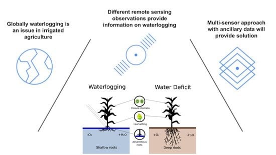
Satellite remote sensing has the potential to monitor and identify waterlogging in agricultural fields. However, there is limited research available on waterlogging within the remote sensing community [31,32,33]. Literature focussed on waterlogging in irrigated agriculture is even more limited [34,35]. Therefore, the aim of this research is to provide a perspective on how waterlogging could be monitored in irrigated agriculture. This article starts by reviewing literature on the topic of waterlogging within the disciplines of agronomy and hydrology. Then, we look at what has been done so far in terms of waterlogging in satellite remote sensing. Here, we will also discuss the presence of waterlogging in current remote sensing-based evaporation algorithms. Throughout the article we use an irrigated sugarcane plantation in Xinavane, Mozambique as a case study. The plantation has waterlogging issues throughout the estate and provides an excellent opportunity to demonstrate how waterlogging is detectable in different remote sensing products. Next, we review approaches that have proved successful in the field of inundation detection and discuss how they might be adapted to address the challenges associated with monitoring waterlogging in irrigated agriculture. Finally, these aspects will be synthesized to present a roadmap towards the development of a methodology to monitor waterlogging with remote sensing for sustainable irrigated agriculture.
2. Waterlogging and Its Impact
Waterlogging is the accumulation of excess water in the rootzone [36]. Agronomists also define soil submergence, where even the aerial (above-ground) plant tissue is partly or completely flooded [37]. When a soil is waterlogged or submerged, pores are predominantly filled with water. However, to sustain proper crop growth a good soil needs to consist of a combination of soil, air, and water. Both waterlogging and soil submergence can create a situation where there is less than 21 percent oxygen in the soil, this is called hypoxia [37,38]. Anoxia occurs when there is a complete absence of oxygen [39].
The response of crops to (partial) submergence or waterlogging differs [40]. In general, when plants are partially submerged, shoot elongation may be suppressed to keep carbohydrates for when flooding disappears. On the other hand, when a plant is fully submerged, rapid elongation can occur to reach the surface of the water. The influence of waterlogging, partial submergence, and full submergence all negatively affect the yield. Here, we define waterlogging as the situation where the rootzone is deprived of oxygen, irrespective of partial or full submergence.
The absence or scarcity of oxygen under waterlogged soil conditions hampers the gas exchange in and around the plant, as water slows down the gas diffusion necessary for major physiological processes in the plant [38]. Vital processes such as photosynthesis and transpiration are heavily affected by waterlogging as these require exchange with atmospheric gases [38,39]. The absence of oxygen inhibits or prevents the roots from taking up ions. This disturbs the water potential in the cells of the plant and leads to a decrease in stomatal conductance (the degree of stomatal opening) [41].
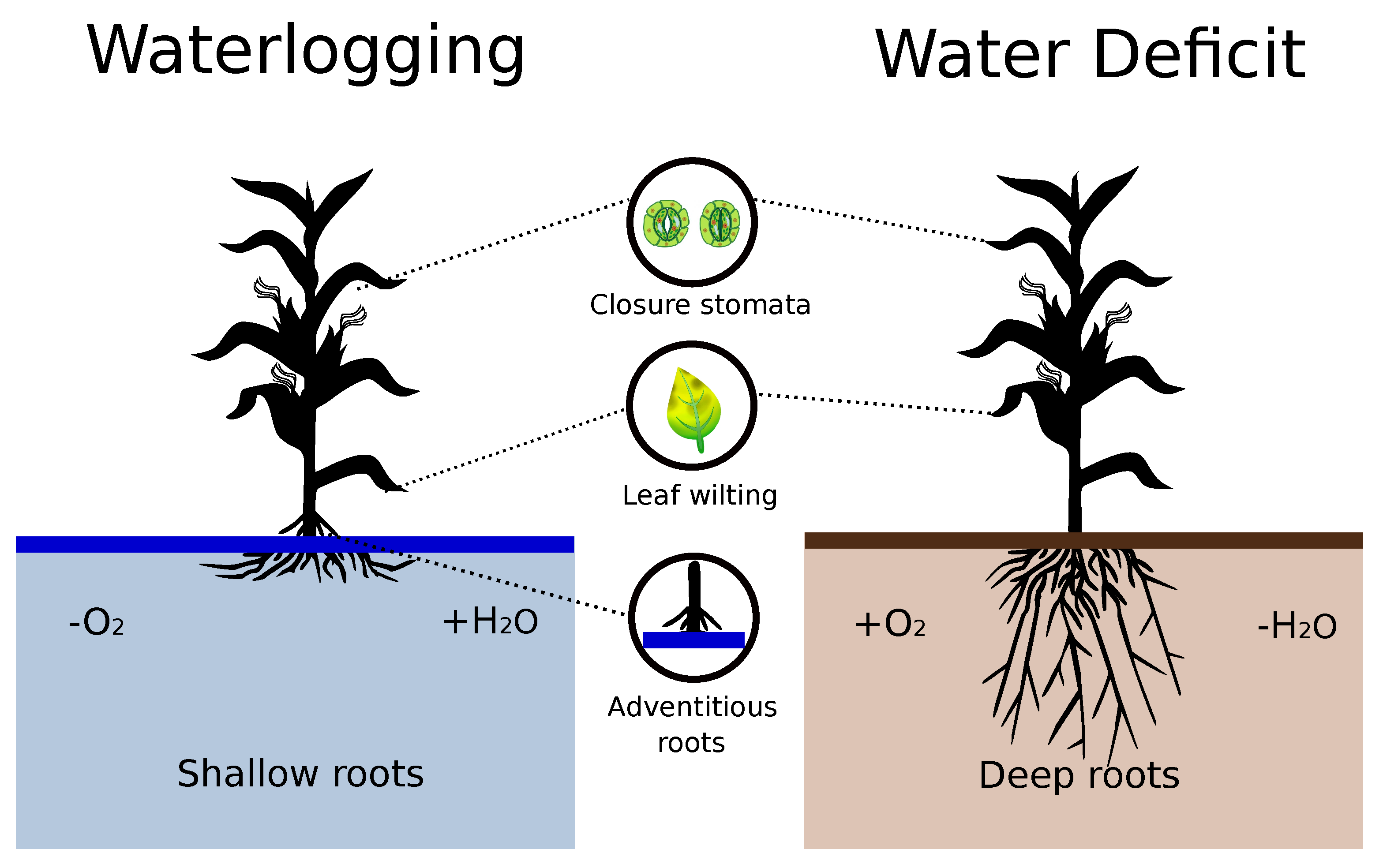
There are many effects of physiologic and morphological responses to oxygen deficit to aerial plant tissue, and they are crop- and variety-dependent. Generally, above-ground symptoms of waterlogging include wilting of the plant, leaf yellowing, reduction of plant growth, and grain yield [3,42]. Importantly, leaf wilting of the plant is often interpreted as water deficit stress [3]. Morphological adaptations or symptoms as stomatal closure or leaf wilting can occur both under crop stress due to water deficit as well as due to waterlogging, see Figure 1.
Waterlogging inhibits root development, leading to a decrease of root length and weight [43]. Ultimately, the damage to the root system negatively impacts the nutrient and water uptake of the crop, and may result in a physiological water deficit above ground [44]. To survive waterlogged soil conditions crops can develop adventitious roots [45]. The adventitious roots grow from the stem and closer to the surface in order to access oxygen [42].
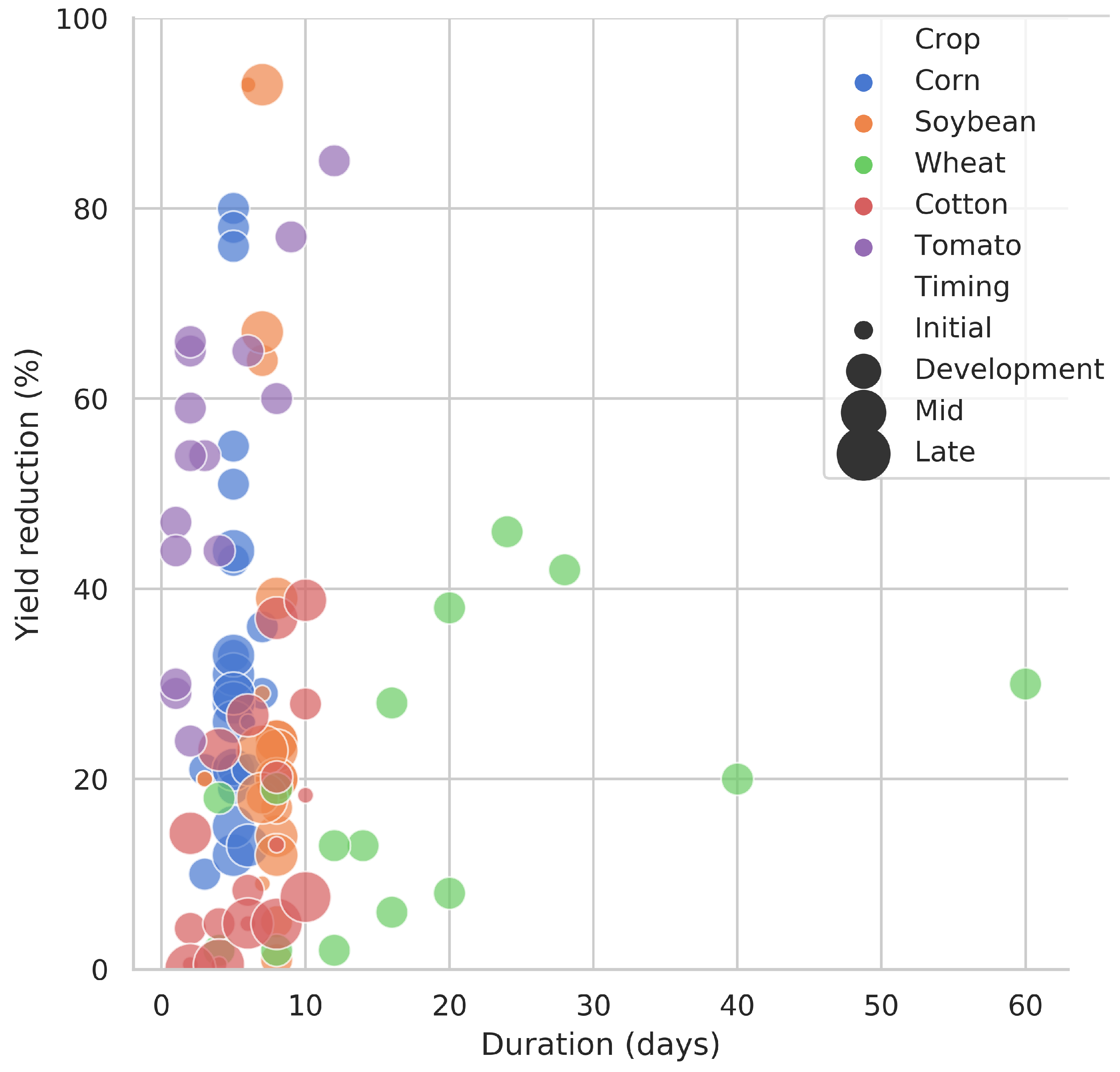
The impact of waterlogging on crop yields can vary in different regions due to the variation in climatic conditions, soil types, crop type, crop variety, crop age, and management differences [42]. Each crop and variety responds differently to waterlogging, and the duration of waterlogging is key to the impact on crop yield [41]. Figure 2 provides an overview of the effect of waterlogging duration on the yield for different major crops based on data collated from the literature. Raw data can be found in Appendix A.
From Figure 2 it can be observed that the selected crops experience a reduction in yield when waterlogging occurs. Most terrestrial crops are sensitive to water excess in the rootzone [38]. However, some crop types are more resistant to waterlogging than others. For example, a few study results on wheat show a yield reduction of 30 percent where waterlogging prevailed for 60 days [46,47,48]. On the other hand, most tomato varieties already experience severe yield reduction after a few days of waterlogging [49,50,51].
Please note that the effect of duration can differ for the same crop type in Figure 2 as some experiments use different varieties or a different onset of waterlogging within the growing season. In all development stages waterlogging is an issue. However, the impact differs because of different coping mechanisms in the crop stages [42,43]. For example, the impact of waterlogging on corn and soybean growth is largest in the initial or development stage [52,53,54,55,56,57]. Germination and seedling establishment are frequently mostly impacted by waterlogging [42].
There are also crops more resistant to waterlogging. For instance, paddy rice is cultivated on flooded soils. However, when completely submerged, paddy rice yield may be negatively affected [41]. Another example of a waterlogging-resistant crop is sugarcane, which can withstand weeks of waterlogging or inundation [27,58]. Nonetheless, long-term or permanent waterlogging is detrimental to sugarcane productivity and can result in secondary soil salinization [59,60].
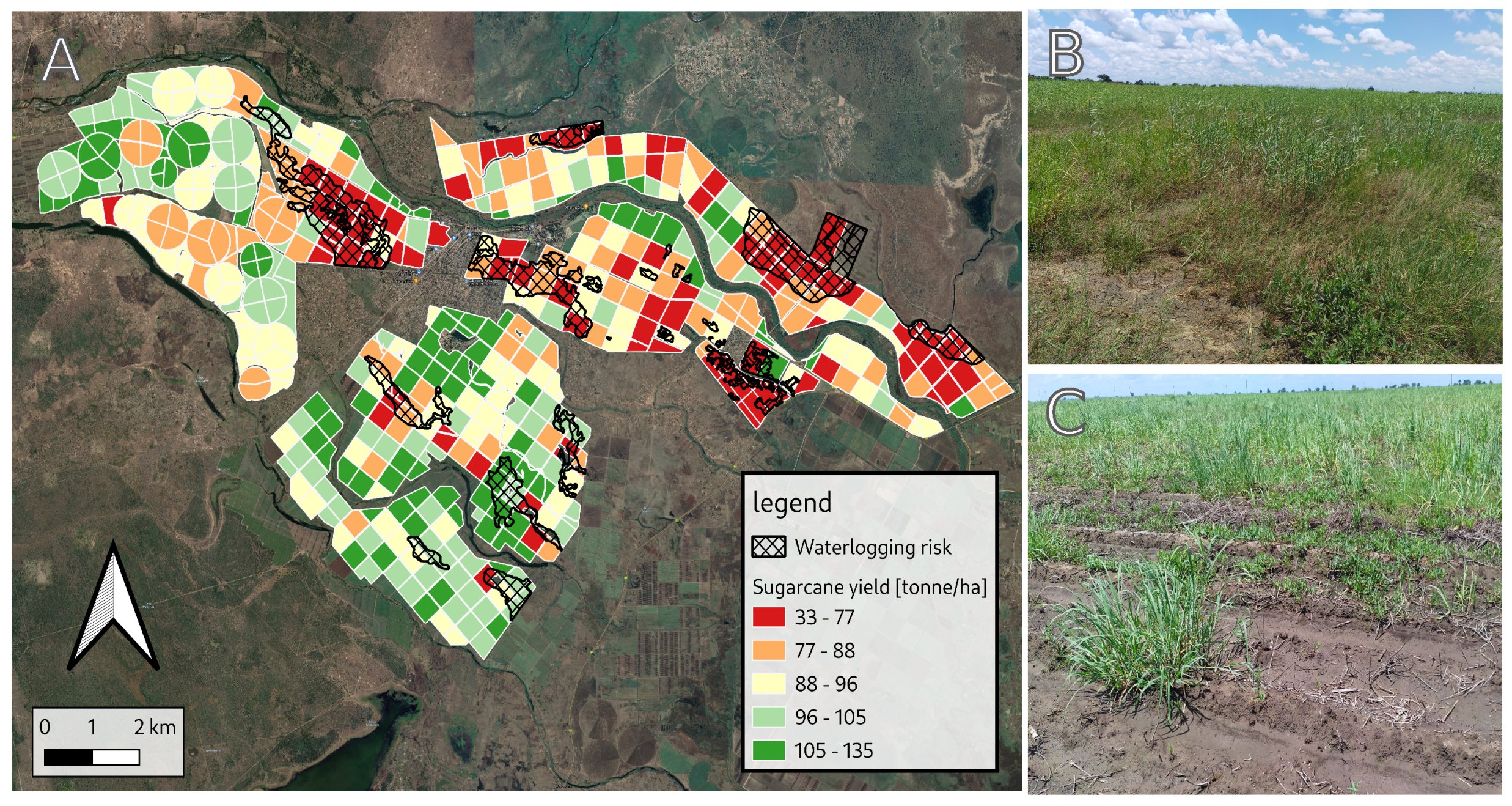
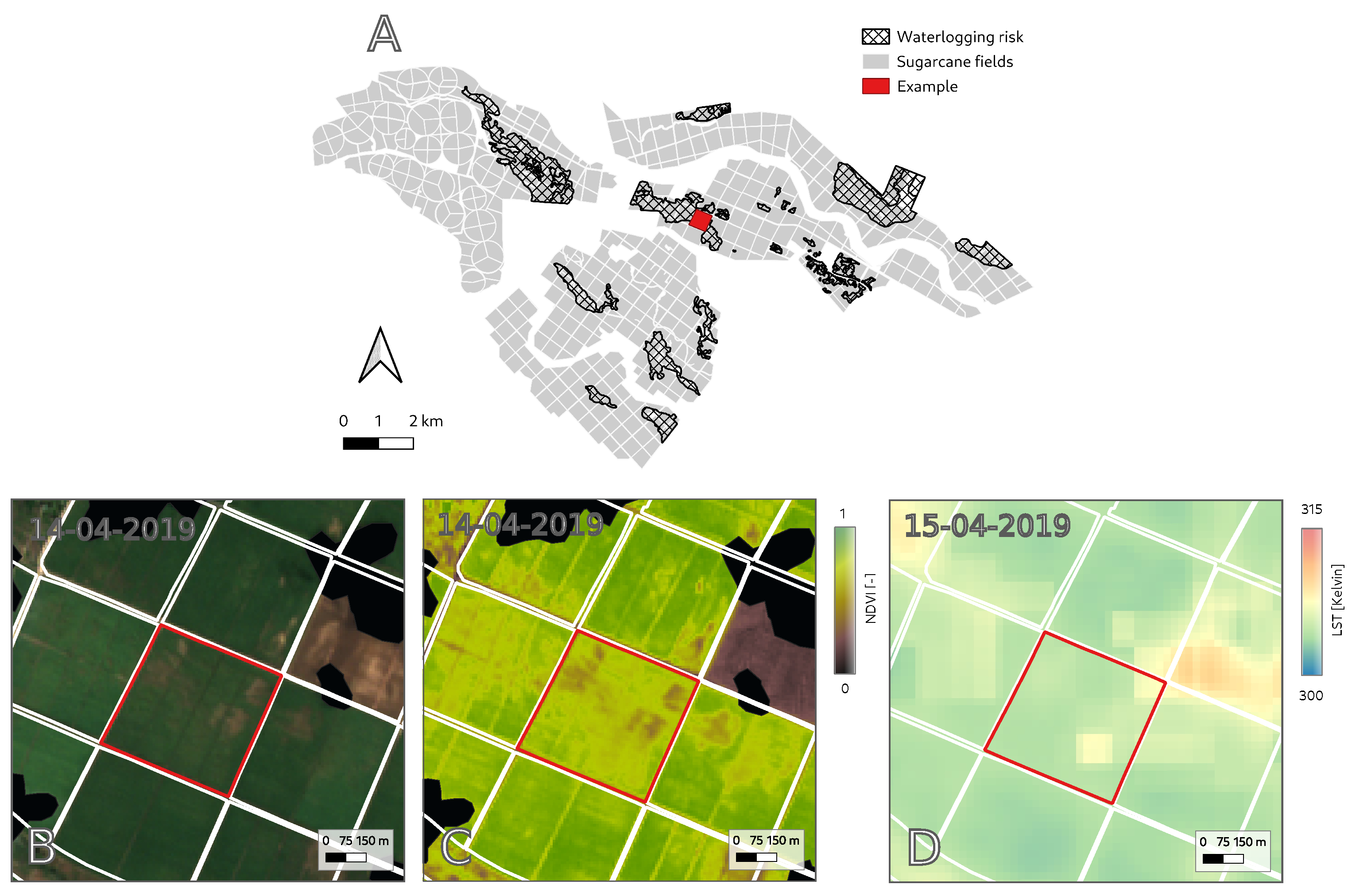
An example of the effects of waterlogging to crop productivity can be observed in an irrigated sugarcane plantation in Xinavane, Mozambique, see Figure 3A–C. In this plantation, there are a lot of productivity issues associated with waterlogging [61,62]. During a large soil survey waterlogged areas were documented [62]. From Figure 3A it is visible that the majority of the waterlogged areas coincide with low crop productivity. Figure 3B,C show photographs of the waterlogged areas. The photographs show how sugarcane growth is hampered as a result of waterlogging.
Waterlogging is also noted as a driver behind yield instability in other areas [63]. Martinez-Feria and Basso [63] assess temporal yield variability in maize, soybean, wheat and cotton in the US Midwest. They prove largest in-field variability can be found in depressional areas, where waterlogging occurs in wet years.
For the majority of the experimental results in Figure 2, the focus lies on the effect of waterlogging with a duration of <10 days to assess the impact on yield. The effect on crop yield can already be significant in a few days. Therefore, both transient or permanent waterlogging needs to be monitored and prevented for optimal crop productivity. Monitoring waterlogging is especially useful in areas where it can be controlled, such as in irrigated or drainage agriculture.
The spatial extent of waterlogging varies from small-scale depressions to large-scale shallow groundwater tables. Waterlogging is related to absence of or limited drainage, and occurs in local depressions, poorly constructed irrigation schemes, (irrigated) wetlands, or areas with impermeable soils, for example [64]. Small-scale depressions in a field may induce waterlogging, but a shallow groundwater table may also enhance the development of waterlogged soils. To prevent or mitigate waterlogging adequate drainage is required [11,64].
Geographically, waterlogging occurs in both natural and human induced circumstances. In natural circumstances, waterlogging may occur when there is a high water table and water is continuously or at once added to the surface by rain or a flood event [3]. These naturally waterlogged areas can be found globally in wetlands, river basins, or lakesides, for example [65]. Waterlogging may also be caused by human interventions such as irrigation, wrongly designed drainage methods, and other surface alterations (e.g., ridges) [65,66]. Due to continuous irrigation, waterlogging is prevalent in agricultural areas in mostly arid and semi-arid areas where irrigation is needed to sustain agricultural production.
Previous research within hydrology and agronomy focused on modeling and monitoring waterlogging in irrigated agriculture to optimize crop productivity. For example, the crop models SWAGMAN, DRAINMOD, and APSIM take the effect of water excess stress on crop yield into consideration in agricultural management [3]. Recently, efforts were made to model waterlogging in irrigated paddy rice to understand human interventions in the irrigation schemes and the resulting yield reduction of waterlogged area [66]. To simulate waterlogging in irrigated agriculture, natural processes need to be considered, but also the hydraulic structures created by humans and the interventions taken place within the system are of importance (e.g., irrigation, gates) [66]. The model developed by Chen et al. [66] is able to predict accurate water levels within the irrigated rice system, but it requires a lot of data. Moving towards an operational monitoring system for waterlogging, satellite remote sensing could provide a less data-intensive solution. There is need for an operational monitoring system that identifies waterlogged areas to support decision-making in irrigation scheduling, drainage, or crop selection [3,66].
3. Waterlogging and Satellite Remote Sensing
There is limited research on waterlogging within the remote sensing community [31,32,33], especially in an irrigation context [34,35]. Within the agricultural water management community, Singh [9] reviewed literature to analyze the applications and GIS techniques available for the management of water in irrigated agriculture. Most of the techniques available focus on delineation of waterlogged areas, where the use of optical data in these studies are common. For example, Choubey [33] uses the infra-red band to delineate waterlogged areas. Normalized Difference Vegetation Index (NDVI) and Normalized Difference Water Index (NDWI) are also common indices used to delineate waterlogged areas [32,34,67,68]. Ultimately, the results are generally static risk maps delineating perennial and/or permanent waterlogged areas. The analysis of temporal variation in, for example, Enhanced Vegetation Index (EVI) or Land Surface Temperature (LST), are particularly useful for identifying waterlogged croplands [69].
The use of Digital Elevation Models (DEM), with or without the combination of optical data, has also played a role in research on delineation of waterlogging within remote sensing [32,35]. El Bastawesy and Ali [35] mapped waterlogging hazard with the help of hydrological parameters analyzed with GIS. A DEM was used to visually interpret the natural sinks in the area under study. Another example is Singh and Pandey [32], where the extent of waterlogging is spatially analyzed with Modified Normalized Difference Water Index (MNDWI) and a DEM.
However, as pointed out in Section 2, waterlogging is a process that changes in space and time in response to physical surface changes, precipitation and/or irrigation application. The aforementioned studies result in delineation of waterlogged areas, but do not monitor the actual areas subject to waterlogging over time. Ideally, an operational system should track the extent of area waterlogged in time. This is essential to provide agriculturalists with timely information on land trafficability and drainage to support decisions related to crop choice and land management practices. Furthermore, information on the waterlogging state is essential to correctly identify the underlying source of crop stress, and to improve irrigation advice based on satellite-based evaporation models [3,61].
Several researchers have demonstrated the potential of satellite remote sensing for irrigation scheduling, but also to assess the water use on global and catchment scale [22,70]. Examples of remote sensing-based evaporation algorithms can be found in Table 1. Table 1 shows that several of these methodologies are now downscaled to fine spatial and temporal resolution with the help of data from new satellites or improved algorithms [71,72]. This opens up an era of research to integrate valuable remote sensing information for field-scale water management [70].
In all remote sensing-based evaporation algorithms in Table 1, crop stress is directly or indirectly incorporated through satellite data by spectral indices, thermal bands, or passive microwave observations. The observed crop stress includes all kinds of crop stresses, such as water stress [73], nutrient stress [74], or stress resulting from disease or pest [29]. In current remote sensing-based evaporation calculations any kind of crop stress will translate into a need for irrigation.
However, waterlogging will also result in the closure of stomata or leaf wilting (see Figure 1), which in turn affects the surface temperature or eventually NDVI observed by the satellite [30]. In current evaporation algorithms, there is a dominant focus on water deficit, and stress resulting from water-logging may be overlooked or misinterpreted as water deficit stress. Scientific reviews on remotely sensed evaporation algorithms for irrigation focus mainly on water deficit stress [22,26,75,76,77,78], and do not consider stress resulting from waterlogging. If such algorithms would be used for irrigation scheduling, this might in fact worsen waterlogging problems [30].
To illustrate this, the irrigated sugarcane plantation in Xinavane, southern Mozambique, is considered. Many fields in the plantation are burdened by permanent waterlogging, see Figure 4. Figure 4B–D give a snapshot of an optical (RGB, Sentinel-2B), NDVI (Sentinel-2B), and Thermal image (B10, Landsat-8) in a field where waterlogging is occurring on the particular dates displayed [79]. From groundwater and field observations the centred field in Figure 4B–D is waterlogged: groundwater levels are within the rootzone and the centre of the field is fully submerged [79]. From Figure 4B you can see the effects of permanent waterlogging (and soil salinization): in some parts the sugarcane is barely growing. The latter is also visible in Figure 4C,D. The parts where sugarcane is barely growing results in a lower NDVI and higher surface radiometric temperature due to the exposure of bare soil.
Thermal Infrared bands and NDVI are common and important building blocks for ET algorithms, see Table 1. Often the surface radiometric temperature is partitioned using NDVI/LAI to retrieve soil and canopy temperature which are crucial to calculate latent heat. However, in the case of waterlogging underneath a canopy the algorithm will be able to visualize the effects of waterlogging only once the adverse effects of waterlogging already occurred. Namely when the NDVI/LAI is low due to hampered crop growth (see bare soil spots Figure 4C).
The latter example is illustrative of how waterlogging can be overlooked or misinterpreted as water deficit stress when these algorithms are used for irrigation. Nevertheless, it is important to include waterlogging stress to inform sustainable irrigation water use and productivity. In this context, Jones [30] also pointed out that it is critical to distinguish water deficit-related stomatal closure from the responses to other stress, which can also lead to stomatal closure. Therefore, monitoring waterlogging can be of help to interpret evaporation algorithms in irrigated agriculture.
4. Detection of Waterlogging with Different Remote Sensing Techniques
Detection of surface water with satellite remote sensing is based on the difference between radiometric properties and temperature of water and other surfaces [94]. There are several theoretical possibilities to detect surface water or waterlogging with satellite data: using passive microwave sensors, optical (VIS) or Near-infrared sensors (NIR), Synthetic Aperture Radar (SAR), or scatterometry. The advantages and disadvantages of each of the first three techniques to detect waterlogging with satellite imagery will be assessed. A summary can be found in Table 2.
First, waterlogging can be detected by passive microwave frequencies [95,96,97]. By combining data from different wavelengths, polarizations, and/or viewing angles, it is possible to retrieve information of the soil surface. Due to the high contrast in dielectric properties between water and dry soil, microwave observations are particularly suitable for sensing water in the topsoil or on the surface [98].
Passive microwave observations show sensitivity to the underlying surface wetness that enables detection of surface water even in densely vegetated areas [96,99,100,101,102]. The polarization difference increases with increasing soil wetness [100]. For example, soil moisture to a depth of 0.8 mm can be sensed with the Ka-band (37 Ghz) frequency [103]. A combination of different frequencies has also been used to detect surface wetness [104].
Higher frequency passive microwave channels, such as Ka-band, are partly influenced by atmospheric circumstances and vegetation and ideally should be corrected for those [105]. Low frequency passive microwave channels, such as the L-band radiometer on SMOS and SMAP, are less affected by canopy and atmospheric conditions [106] and are well suited to soil moisture monitoring.
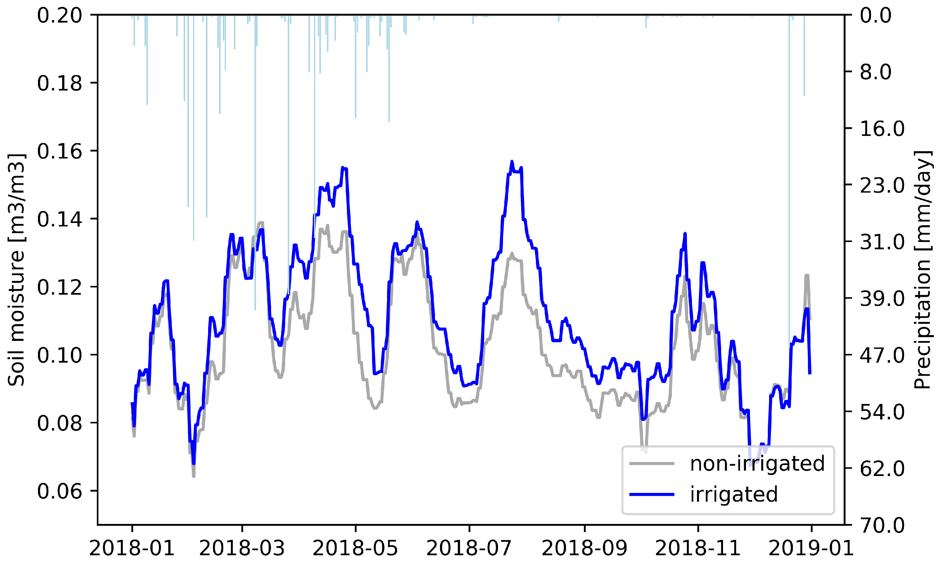
The difficulty in using passive microwave observations to detect waterlogging is that their resolution is coarse. Observations at lower frequencies have a lower spatial resolution than observations at higher frequencies (e.g., L-band’s spatial resolution is in the order of 36 km). There are operational products that downscale brightness temperature observations. For example, NASA provides a downscaled 9 km resolution brightness temperature and soil moisture product [107]. This enhanced L-band product has, to our knowledge, not yet been used in research to detect surface water.
To illustrate the potential value of passive microwave remote sensing here, Figure 5 shows a comparison of satellite derived soil moisture from L-band observations over the sugarcane plantation in Xinavane and from a reference area with no irrigation. Here a downscaled version of SMAP L-band observations based on a new deconvolution method [108] and converted to soil moisture with the Land Parameter Retrieval Model gridded at 100 m is used [109]. Outside of the rainy season the average soil moisture is higher than the reference area without irrigation. Despite the coarse spatial resolution, L-band passive microwave observations are capable of detecting differences in surface soil moisture even under the dense sugarcane canopy.
Secondly, it is possible to detect surface water with VIS and NIR sensors. The physical radiation over different wavelengths in the VIS and NIR domain are distinctly different for water, compared to other surfaces. Longer wavelengths in the VIS and NIR bands are absorbed more by water than shorter VIS. Due to these spectral response patterns, water bodies can be delineated per pixel [110]. In addition, VIS and NIR sensors observe at a high spatial resolution, e.g., Sentinel-2 at a 10 m spatial resolution [111].
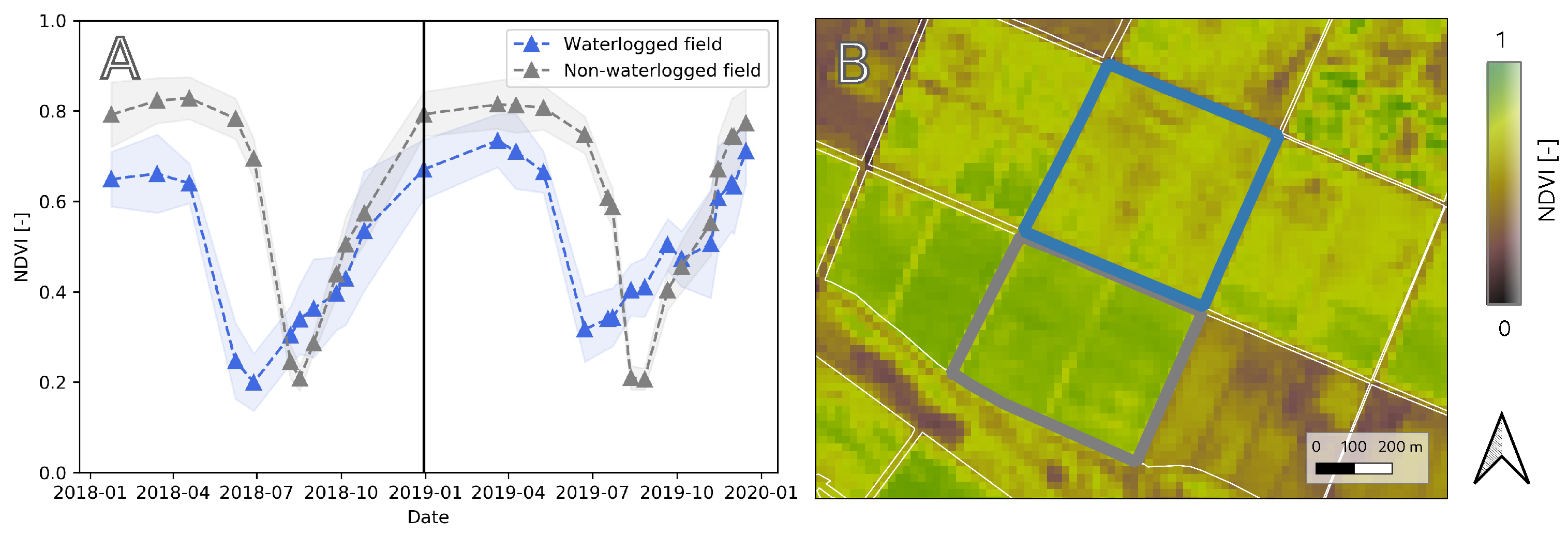
Nevertheless, Figure 6A shows a NDVI time-series (Sentinel-2) of a water logged and non-waterlogged field in the sugarcane plantation Xinavane, Mozambique (See Figure 3). The NDVI values in the timeseries of the waterlogged field are lower compared to the non-waterlogged field, as a result of hampered crop growth due to waterlogging. This confirms there is information within the optical spectrum on waterlogging. In addition, the standard deviation in the field dealing with waterlogging is larger. The latter is visible in Figure 6B, where a snapshot of the two fields show the waterlogged field (blue) shows less uniformity than the non-waterlogged field (gray).
A limitation of this technique is the inability to acquire observations under cloudy conditions [112]. Since waterlogging may also result from intensive rainfall events, the inability to have observations under cloudy conditions hampers the ability to continuously monitor waterlogging. In addition, VIS and NIR data are sensitive to the reflectance at the top of the canopy and cannot penetrate a dense canopy to provide information from the underlying surface [110]. This is highly problematic in agricultural applications where we need to monitor the surface under crops.
Third, active microwave observations may also provide information on waterlogging. SAR transmits a microwave pulse and measures the backscattered power of each returning signal [110]. These observations can be obtained in different wavelengths and polarizations. Generally, open water surfaces are distinguished by low backscattering coefficients [94]. Data from SAR are able to detect surface water bodies underneath vegetation [113,114]. For example, SAR can detect water beneath a slender leaf crop such as rice [114]. However, the signal is influenced by vegetation and the signal saturates under a thick canopy [115].
Unlike VIS and NIR data, SAR data are less influenced by atmospheric effects and observations can be made on cloudy days [112]. In addition, SAR provides data at high spatial resolution. Sentinel-1, for instance, provides SAR backscatter at a 5 × 20 m resolution [116]. Sentinel-1 data have a revisit time of six days with platform A and B, but coverage varies around the globe. For example, for the sugarcane plantation in Xinavane there is an observation every 12 days. To observe waterlogging, however, high temporal resolution is required, since most terrestrial crops are negatively effected by waterlogging in a matter of days (see Section 2).
The spatial and temporal resolutions of current available satellite products will limit the operationability of monitoring waterlogging in irrigated agriculture. Future missions, with higher spatial and temporal resolutions can become game-changers in the future. For example, ESA’s ROSE-L mission will provide high spatial and temporal resolution L-band data that is especially of interest to flood mapping, in particular below vegetation [117]. Additionally, Global Navigation Satellite Systems - Reflectometry (GNSS-R) signals can be an interesting data source to monitor waterlogging [118].
Several sources of remote sensing data contain useful information on waterlogging. Combining them provides complementary information on waterlogging at a range of spatial and temporal scales, and provides a way to circumvent the limitations of the individual data streams.
5. Downscaling Using Ancillary Data
In addition to combining observations from different parts of the electromagnetic spectrum, the use of ancillary data can provide a means to downscale passive microwave observations to higher spatial resolutions needed to monitor within-field waterlogging. In this regard, future research on monitoring waterlogging can benefit from the work done so far within monitoring inundation. Recently (global) inundation products were introduced that combine different satellite products with passive microwave remote sensing, also referred to as hybrid approaches [94,119,120]. By combining different satellite products, different sensitivities to surface properties are differentiated, but also higher spatial resolutions are obtained [112]. Two examples are Global Inundation Extent from Different Satellites (GIEMS) and Surface Water Microwave Product Series (SWAMP) [119,121].
Table 3 gives an overview of the characteristics of these inundation products. In recent years several researchers have attempted to downscale global and regional surface water products to higher spatial resolutions [94,120,122,123]. These methodologies all require high resolution ancillary data to improve the resolution of the passive microwave observations. Prigent et al. [94] distinguishes two strategies to improve the resolution of coarse scale surface water products: (1) downscaling using high spatial resolution satellite observations; (2) downscaling using topography information. Although waterlogging requires even higher spatial and temporal resolutions, these existing methodologies set a basis for an approach to monitor waterlogging.
In these inundation products the underlying assumption is the passive microwaves signal used is linked to the fraction of land inundated [94,120,124]. However, in irrigated agriculture there is a very important additional driver besides topography and precipitation, namely irrigation and man-made drainage. The underlying assumption used in current inundation models need to add derivatives of irrigation effects or detection of irrigation in order to monitor waterlogging.
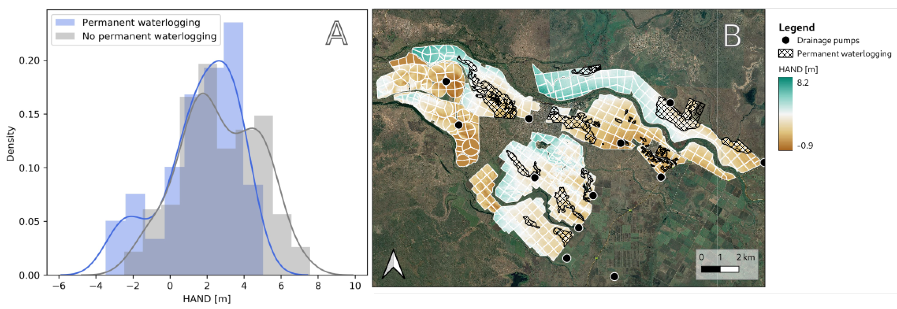
To monitor waterlogging future studies should focus on how to include human-made drivers inducing waterlogging. Future scientific studies need to focus on using: (1) monitoring waterlogging with ancillary data by looking at derivatives of irrigation, and (2) waterlogging occurrence from drainage parameters deducted from high spatial resolution DEMs. These DEMs can be developed with data from LiDAR or Unmanned Aereal Vehicles (UAVs). A determining factor in suitability for DEM to monitor waterlogging is the vertical accuracy, which is still too large in available global satellite products, e.g., TanDEM-X with a vertical accuracy of two meters [126].
For example, in the sugarcane plantation in Mozambique permanently waterlogged areas occur in poorly drained areas, see Figure 7. The Height Above Nearest Drainage (HAND) was computed with a DEM from LiDAR observations. LiDAR data were provided by the agricultural department of the plantation and acquired between 17 and 27 September 2015. LiDAR return points were classified as ground or non-ground, where the ground points were correlated with Ground Control Points (GCP) to create a DEM. The Root Mean Square error between the return points and GCP was 0.04 m. For Figure 7A a DEM with a spatial resolution of 13 by 13 m was used. To compute the HAND model, the height of the drainage point of each irrigation section was subtracted from the height of the other points in the irrigation section catchment. Figure 7 shows the distribution of HAND is different in waterlogged fields compared to non-waterlogged fields. This illustrates topographical information withholds information on waterlogging or the potential to be waterlogged [124].
6. Conclusions
Waterlogging is a localized phenomenon (e.g., ponds within a field) and can induce crop stress within a few days. Within agronomy, studies on crop stress focus more on water deficit stress, as compared to stress resulting from waterlogging. However, waterlogging is a common and adverse problem in (irrigated) agriculture. Most terrestrial crops are susceptible to waterlogging, but the intensity of the negative effects depend on crop type and variety, duration, timing, among other factors. Within (irrigated) agriculture, waterlogging needs to be prevented to optimize yield, water productivity, and soil quality. Furthermore, failure to tackle persistent waterlogging can induce secondary soil salinization, a process that is hard to reverse.
The above-ground effect of waterlogging on crops is hard to distinguish from water deficit stress, as responses such as stomatal closure and leaf wilting occur in both situations. Currently the origin of crop stress is not distinguished by remote sensing-based evaporation algorithms and these may therefore be erroneously interpreted as a need for irrigation. In sum, before evaporation estimates from satellite data can play a role in optimizing the field-scale water use in irrigated areas, evaporation algorithms must be able to identify water stress only in the case of a water deficit in the root-zone. Here, monitoring waterlogging can play a role.
Efforts in modelling waterlogging are data-intensive and it is worthwhile to explore whether satellite remote sensing provides opportunities for an operational system to monitor waterlogging. In recent years studies within remote sensing on irrigated agriculture have focussed on static delineation of waterlogging. However, waterlogging is a dynamic process that requires frequent monitoring. Future research to create a remote sensing-based monitoring system to prevent waterlogging can learn from research on the remote sensing of inundation.
To demonstrate the information on waterlogging present in different remote sensing data products, we use an irrigated sugarcane plantation in Xinavane, Mozambique, as a case study. The plantation faces issues with waterlogging and, therefore, use the information to illustrate how different sensing techniques may contain information on waterlogging. However, each sensing technique has its own limitations. Consequently, there is not just one sensing technique suitable to monitor waterlogging. Opportunities to monitor waterlogging lie in hybrid approaches combining different satellite products to optimize temporal and spatial resolution. Future scientific routes should focus on complementing remote sensing data with ancillary data, and waterlogging occurrence from drainage parameters deduced from high spatial resolution DEMs (with LiDAR or UAVs).
Remote sensing can be used to identify areas that are frequently subject to waterlogging, information that can be used to make smarter crop choices and to improve drainage. Remote sensing data from multiple sources can be combined with ancillary data to monitor transient waterlogging at high temporal and spatial resolution. This can provide real-time information on trafficability, and potential crop damage. Most importantly, this provides an essential input to evaporation estimation algorithms used for irrigation support. In addition to conserving water resources, the correct attribution of crop stress to waterlogging rather than water deficit stress would ensure that waterlogging is not further exacerbated by the application of additional irrigation.
Funding
We would like to thank the Netherlands Enterprise Agency for subsidizing the IWACA-Tech project, which this work was part of.
Institutional Review Board Statement
Not applicable.
Informed Consent Statement
Informed consent was obtained from all subjects involved in the study.
Data Availability Statement
Data is available upon request.
Acknowledgments
The authors would like to thank the agricultural department of Tongaat Hulett in Xinavane for the pleasant collaboration and sharing of ground data. In addition, the authors would like to thank Milton Paulao Acua and Kathelijne Beenen who were involved during the project IWACA-Tech, they helped during a fieldwork and creating a DEM.
Conflicts of Interest
The author declares no conflict of interest.
Appendix A

Table A1.
Different field studies researching the effect of waterlogging on crop productivity. The information in the table was used to create Figure 2. Timing refers to crop stage of the onset of waterlogging.
Table A1.
Different field studies researching the effect of waterlogging on crop productivity. The information in the table was used to create Figure 2. Timing refers to crop stage of the onset of waterlogging.
| Crop | Location | Timing | Duration (Days) | Yield Reduction (%) | Reference |
|---|---|---|---|---|---|
| Corn | Missouri, USA | Development | 3 | 10.0 | Kaur et al. [53] |
| Corn | Missouri, USA | Development | 7 | 29.0 | Kaur et al. [53] |
| Corn | Missouri, USA | Development | 3 | 21.0 | Kaur et al. [53] |
| Corn | Missouri, USA | Development | 7 | 36.0 | Kaur et al. [53] |
| Corn | Varanasi, India | Development | 5 | 21.0 | Shah et al. [52] |
| Corn | Varanasi, India | Development | 5 | 19.0 | Shah et al. [52] |
| Corn | Varanasi, India | Development | 5 | 51.0 | Shah et al. [52] |
| Corn | Varanasi, India | Development | 5 | 55.0 | Shah et al. [52] |
| Corn | Varanasi, India | Development | 5 | 33.0 | Shah et al. [52] |
| Corn | Varanasi, India | Development | 5 | 43.0 | Shah et al. [52] |
| Corn | Varanasi, India | Development | 5 | 80.0 | Shah et al. [52] |
| Corn | Varanasi, India | Development | 5 | 21.0 | Shah et al. [52] |
| Corn | Varanasi, India | Development | 5 | 78.0 | Shah et al. [52] |
| Corn | Varanasi, India | Development | 5 | 76.0 | Shah et al. [52] |
| Corn | Varanasi, India | Mid | 5 | 12.0 | Shah et al. [52] |
| Corn | Varanasi, India | Mid | 5 | 15.0 | Shah et al. [52] |
| Corn | Varanasi, India | Mid | 5 | 29.0 | Shah et al. [52] |
| Corn | Varanasi, India | Mid | 5 | 31.0 | Shah et al. [52] |
| Corn | Varanasi, India | Mid | 5 | 21.0 | Shah et al. [52] |
| Corn | Varanasi, India | Mid | 5 | 28.0 | Shah et al. [52] |
| Corn | Varanasi, India | Mid | 5 | 44.0 | Shah et al. [52] |
| Corn | Varanasi, India | Mid | 5 | 26.0 | Shah et al. [52] |
| Corn | Varanasi, India | Mid | 5 | 33.0 | Shah et al. [52] |
| Corn | Varanasi, India | Mid | 5 | 29.0 | Shah et al. [52] |
| Corn | Shandong, China | Initial | 6 | 26.0 | Ren et al. [54] |
| Corn | Shandong, China | Development | 6 | 21.0 | Ren et al. [54] |
| Corn | Shandong, China | Mid | 6 | 13.0 | Ren et al. [54] |
| Soybean | Missouri, USA | Mid | 8 | 14.0 | Rhine et al. [55] |
| Soybean | Missouri, USA | Mid | 8 | 20.0 | Rhine et al. [55] |
| Soybean | Missouri, USA | Development | 8 | 5.0 | Rhine et al. [55] |
| Soybean | Missouri, USA | Mid | 8 | 24.0 | Rhine et al. [55] |
| Soybean | Missouri, USA | Development | 8 | 17.0 | Rhine et al. [55] |
| Soybean | Missouri, USA | Mid | 8 | 24.0 | Rhine et al. [55] |
| Soybean | Missouri, USA | Mid | 8 | 39.0 | Rhine et al. [55] |
| Soybean | Missouri, USA | Mid | 8 | 23.0 | Rhine et al. [55] |
| Soybean | Missouri, USA | Development | 8 | 1.0 | Rhine et al. [55] |
| Soybean | Missouri, USA | Mid | 8 | 12.0 | Rhine et al. [55] |
| Soybean | Missouri, USA | Mid | 8 | 20.0 | Rhine et al. [55] |
| Soybean | Ohio, USA | Initial | 3 | 20.0 | Sullivan et al. [56] |
| Soybean | Ohio, USA | Initial | 3 | 20.0 | Sullivan et al. [56] |
| Soybean | Ohio, USA | Initial | 6 | 93.0 | Sullivan et al. [56] |
| Soybean | Ohio, USA | Initial | 6 | 93.0 | Sullivan et al. [56] |
| Soybean | Louisiana, USA | Initial | 7 | 29.0 | Linkemer et al. [57] |
| Soybean | Louisiana, USA | Initial | 7 | 9.0 | Linkemer et al. [57] |
| Soybean | Louisiana, USA | Development | 7 | 18.0 | Linkemer et al. [57] |
| Soybean | Louisiana, USA | Development | 7 | 64.0 | Linkemer et al. [57] |
| Soybean | Louisiana, USA | Mid | 7 | 93.0 | Linkemer et al. [57] |
| Soybean | Louisiana, USA | Mid | 7 | 67.0 | Linkemer et al. [57] |
| Soybean | Louisiana, USA | Late | 7 | 23.0 | Linkemer et al. [57] |
| Soybean | Louisiana, USA | Late | 7 | 18.0 | Linkemer et al. [57] |
| Wheat | Pisa, Italy | Development | 4 | 2.0 | Pampana et al. [46] |
| Wheat | Pisa, Italy | Development | 8 | 2.0 | Pampana et al. [46] |
| Wheat | Pisa, Italy | Development | 12 | 2.0 | Pampana et al. [46] |
| Wheat | Pisa, Italy | Development | 16 | 6.0 | Pampana et al. [46] |
| Wheat | Pisa, Italy | Development | 20 | 8.0 | Pampana et al. [46] |
| Wheat | Pisa, Italy | Development | 40 | 20.0 | Pampana et al. [46] |
| Wheat | Pisa, Italy | Development | 60 | 30.0 | Pampana et al. [46] |
| Wheat | Arkansas, USA | Development | 28 | 42.0 | Arguello et al. [48] |
| Wheat | Arkansas, USA | Development | 14 | 13.0 | Arguello et al. [48] |
| Wheat | Lleida, Spain | Development | 4 | 18.0 | Marti et al. [47] |
| Wheat | Lleida, Spain | Development | 8 | 19.0 | Marti et al. [47] |
| Wheat | Lleida, Spain | Development | 12 | 13.0 | Marti et al. [47] |
| Wheat | Lleida, Spain | Development | 16 | 28.0 | Marti et al. [47] |
| Wheat | Lleida, Spain | Development | 20 | 38.0 | Marti et al. [47] |
| Wheat | Lleida, Spain | Development | 24 | 46.0 | Marti et al. [47] |
| Cotton | Xinxiang, China | Initial | 2 | 0.5 | Wang et al. [127] |
| Cotton | Xinxiang, China | Initial | 4 | 0.5 | Wang et al. [127] |
| Cotton | Xinxiang, China | Initial | 6 | 4.8 | Wang et al. [127] |
| Cotton | Xinxiang, China | Initial | 8 | 13.1 | Wang et al. [127] |
| Cotton | Xinxiang, China | Initial | 10 | 18.3 | Wang et al. [127] |
| Cotton | Xinxiang, China | Development | 2 | 4.3 | Wang et al. [127] |
| Cotton | Xinxiang, China | Development | 4 | 4.8 | Wang et al. [127] |
| Cotton | Xinxiang, China | Development | 6 | 8.3 | Wang et al. [127] |
| Cotton | Xinxiang, China | Development | 8 | 20.2 | Wang et al. [127] |
| Cotton | Xinxiang, China | Development | 10 | 27.9 | Wang et al. [127] |
| Cotton | Xinxiang, China | Mid | 2 | 14.3 | Wang et al. [127] |
| Cotton | Xinxiang, China | Mid | 4 | 23.1 | Wang et al. [127] |
| Cotton | Xinxiang, China | Mid | 6 | 26.7 | Wang et al. [127] |
| Cotton | Xinxiang, China | Mid | 8 | 36.9 | Wang et al. [127] |
| Cotton | Xinxiang, China | Mid | 10 | 38.8 | Wang et al. [127] |
| Cotton | Xinxiang, China | Late | 2 | 0.0 | Wang et al. [127] |
| Cotton | Xinxiang, China | Late | 4 | 0.5 | Wang et al. [127] |
| Cotton | Xinxiang, China | Late | 6 | 4.8 | Wang et al. [127] |
| Cotton | Xinxiang, China | Late | 8 | 4.8 | Wang et al. [127] |
| Cotton | Xinxiang, China | Late | 10 | 7.6 | Wang et al. [127] |
| Tomato | Manikganj, Bangladesh | Development | 3 | 54.0 | Tareq et al. [49] |
| Tomato | Manikganj, Bangladesh | Development | 6 | 65.0 | Tareq et al. [49] |
| Tomato | Manikganj, Bangladesh | Development | 9 | 77.0 | Tareq et al. [49] |
| Tomato | Manikganj, Bangladesh | Development | 12 | 85.0 | Tareq et al. [49] |
| Tomato | Taiwan | Development | 2 | 24.0 | Ezin et al. [50] |
| Tomato | Taiwan | Development | 4 | 44.0 | Ezin et al. [50] |
| Tomato | Taiwan | Development | 8 | 60.0 | Ezin et al. [50] |
| Tomato | Odisha, India | Development | 1 | 29.0 | Mohanty et al. [51] |
| Tomato | Odisha, India | Development | 2 | 65.0 | Mohanty et al. [51] |
| Tomato | Odisha, India | Development | 1 | 47.0 | Mohanty et al. [51] |
| Tomato | Odisha, India | Development | 2 | 59.0 | Mohanty et al. [51] |
| Tomato | Odisha, India | Development | 1 | 30.0 | Mohanty et al. [51] |
| Tomato | Odisha, India | Development | 2 | 54.0 | Mohanty et al. [51] |
| Tomato | Odisha, India | Development | 1 | 44.0 | Mohanty et al. [51] |
| Tomato | Odisha, India | Development | 2 | 66.0 | Mohanty et al. [51] |
References
- Houk, E.; Frasier, M.; Schuck, E. The agricultural impacts of irrigation induced waterlogging and soil salinity in the Arkansas Basin. Agric. Water Manag. 2006, 85, 175–183. [Google Scholar] [CrossRef]
- Wallender, W.W.; Tanji, K.K. Agricultural Salinity Assessment and Management; American Society of Civil Engineers (ASCE): Reston, Virginia, 2011. [Google Scholar]
- Shaw, R.E.; Meyer, W.S.; McNeill, A.; Tyerman, S.D. Waterlogging in Australian agricultural landscapes: A review of plant responses and crop models. Crop. Pasture Sci. 2013, 64, 549–562. [Google Scholar] [CrossRef]
- Dennis, E.S.; Dolferus, R.; Ellis, M.; Rahman, M.; Wu, Y.; Hoeren, F.; Grover, A.; Ismond, K.; Good, A.; Peacock, W. Molecular strategies for improving waterlogging tolerance in plants. J. Exp. Bot. 2000, 51, 89–97. [Google Scholar] [CrossRef] [PubMed]
- FAO. Coping with Water Scarcity in Agriculture a Global Framework for Action in a Changing Climate. 2016. Available online: http://www.fao.org/3/a-i6459e.pdf (accessed on 13 April 2021).
- Steduto, P.; Hoogeveen, J.; Winpenny, J.; Burke, J. Coping with Water Scarcity: An Action Framework for Agriculture and Food Security; Food and Agriculture Organization of the United Nations: Rome, Italy, 2017. [Google Scholar]
- Ward, P.; Dunin, F.; Micin, S. Water use and root growth by annual and perennial pastures and subsequent crops in a phase rotation. Agric. Water Manag. 2002, 53, 83–97. [Google Scholar] [CrossRef]
- Christen, E.W.; Ayars, J.E.; Hornbuckle, J.W. Subsurface drainage design and management in irrigated areas of Australia. Irrig. Sci. 2001, 21, 35–43. [Google Scholar] [CrossRef]
- Singh, A. Hydrological problems of water resources in irrigated agriculture: A management perspective. J. Hydrol. 2016, 541, 1430–1440. [Google Scholar] [CrossRef]
- Poddar, R.; Qureshi, M.E.; Syme, G. Comparing irrigation management reforms in Australia and India—A special reference to participatory irrigation management. Irrig. Drain. 2011, 60, 139–150. [Google Scholar] [CrossRef]
- Valipour, M. Drainage, waterlogging, and salinity. Arch. Agron. Soil Sci. 2014, 60, 1625–1640. [Google Scholar] [CrossRef]
- Neumann, K.; Stehfest, E.; Verburg, P.H.; Siebert, S.; Müller, C.; Veldkamp, T. Exploring global irrigation patterns: A multilevel modelling approach. Agric. Syst. 2011, 104, 703–713. [Google Scholar] [CrossRef]
- You, L.; Ringler, C.; Wood-Sichra, U.; Robertson, R.; Wood, S.; Zhu, T.; Nelson, G.; Guo, Z.; Sun, Y. What is the irrigation potential for Africa? A combined biophysical and socioeconomic approach. Food Policy 2011, 36, 770–782. [Google Scholar] [CrossRef] [Green Version]
- Cassidy, E.S.; West, P.C.; Gerber, J.S.; Foley, J.A. Redefining agricultural yields from tonnes to people nourished per hectare. Environ. Res. Lett. 2013, 8, 034015. [Google Scholar] [CrossRef]
- Mueller, N.D.; Gerber, J.S.; Johnston, M.; Ray, D.K.; Ramankutty, N.; Foley, J.A. Closing yield gaps through nutrient and water management. Nature 2012, 490, 254. [Google Scholar] [CrossRef]
- Pfister, S.; Bayer, P.; Koehler, A.; Hellweg, S. Projected water consumption in future global agriculture: Scenarios and related impacts. Sci. Total. Environ. 2011, 409, 4206–4216. [Google Scholar] [CrossRef]
- Mashnik, D.; Jacobus, H.; Barghouth, A.; Wang, E.J.; Blanchard, J.; Shelby, R. Increasing productivity through irrigation: Problems and solutions implemented in Africa and Asia. Sustain. Energy Technol. Assess. 2017, 22, 220–227. [Google Scholar] [CrossRef]
- FAO. AQUASTAT Main Database, Food and Agriculture Organization of the United Nations (FAO). 2016. Available online: http://www.fao.org/nr/water/aquastat/data/ (accessed on 27 October 2019).
- Fischer, G.; Tubiello, F.N.; Van Velthuizen, H.; Wiberg, D.A. Climate change impacts on irrigation water requirements: Effects of mitigation, 1990–2080. Technol. Forecast. Soc. Chang. 2007, 74, 1083–1107. [Google Scholar] [CrossRef] [Green Version]
- Ferguson, I.M.; Maxwell, R.M. Human impacts on terrestrial hydrology: Climate change versus pumping and irrigation. Environ. Res. Lett. 2012, 7, 044022. [Google Scholar] [CrossRef] [Green Version]
- Bhaduri, A.; Bogardi, J.; Siddiqi, A.; Voigt, H.; Vörösmarty, C.; Pahl-Wostl, C.; Bunn, S.E.; Shrivastava, P.; Lawford, R.; Foster, S.; et al. Achieving sustainable development goals from a water perspective. Front. Environ. Sci. 2016, 4, 64. [Google Scholar] [CrossRef] [Green Version]
- Bastiaanssen, W.G.; Molden, D.J.; Makin, I.W. Remote sensing for irrigated agriculture: Examples from research and possible applications. Agric. Water Manag. 2000, 46, 137–155. [Google Scholar] [CrossRef]
- Atzberger, C. Advances in remote sensing of agriculture: Context description, existing operational monitoring systems and major information needs. Remote Sens. 2013, 5, 949–981. [Google Scholar] [CrossRef] [Green Version]
- Vuolo, F.; D’Urso, G.; De Michele, C.; Bianchi, B.; Cutting, M. Satellite-based irrigation advisory services: A common tool for different experiences from Europe to Australia. Agric. Water Manag. 2015, 147, 82–95. [Google Scholar] [CrossRef]
- Vanino, S.; Nino, P.; De Michele, C.; Bolognesi, S.F.; D’Urso, G.; Di Bene, C.; Pennelli, B.; Vuolo, F.; Farina, R.; Pulighe, G.; et al. Capability of Sentinel-2 data for estimating maximum evapotranspiration and irrigation requirements for tomato crop in Central Italy. Remote Sens. Environ. 2018, 215, 452–470. [Google Scholar] [CrossRef]
- Calera, A.; Campos, I.; Osann, A.; D Urso, G.; Menenti, M. Remote sensing for crop water management from ET modelling to services for the end users. Sensors 2017, 17, 1104. [Google Scholar] [CrossRef] [Green Version]
- Glaz, B.; Morris, D.R.; Daroub, S.H. Sugarcane photosynthesis, transpiration, and stomatal conductance due to flooding and water table. Crop Sci. 2004, 44, 1633–1641. [Google Scholar] [CrossRef] [Green Version]
- Inman-Bamber, N.; Smith, D. Water relations in sugarcane and response to water deficits. Field Crop. Res. 2005, 92, 185–202. [Google Scholar] [CrossRef]
- Franke, J.; Menz, G. Multi-temporal wheat disease detection by multi-spectral remote sensing. Precis. Agric. 2007, 8, 161–172. [Google Scholar] [CrossRef]
- Jones, H. Opportunities and pitfalls in the use of thermal sensing for monitoring water stress and transpiration. Acta Hortic. 2018, 1197, 31–44. [Google Scholar] [CrossRef]
- Mondal, D.; Pal, S. Monitoring dual-season hydrological dynamics of seasonally flooded wetlands in the lower reach of Mayurakshi River, Eastern India. Geocarto Int. 2018, 33, 225–239. [Google Scholar] [CrossRef]
- Singh, S.K.; Pandey, A. Geomorphology and the controls of geohydrology on waterlogging in Gangetic Plains, North Bihar, India. Environ. Earth Sci. 2014, 71, 1561–1579. [Google Scholar] [CrossRef]
- Choubey, V. Detection and delineation of waterlogging by remote sensing techniques. J. Indian Soc. Remote. Sens. 1997, 25, 123–135. [Google Scholar] [CrossRef]
- Chowdary, V.; Chandran, R.V.; Neeti, N.; Bothale, R.; Srivastava, Y.; Ingle, P.; Ramakrishnan, D.; Dutta, D.; Jeyaram, A.; Sharma, J.; et al. Assessment of surface and sub-surface waterlogged areas in irrigation command areas of Bihar state using remote sensing and GIS. Agric. Water Manag. 2008, 95, 754–766. [Google Scholar] [CrossRef]
- El Bastawesy, M.; Ali, R.R. The use of GIS and remote sensing for the assessment of waterlogging in the dryland irrigated catchments of Farafra Oasis, Egypt. Hydrol. Process. 2013, 27, 206–216. [Google Scholar] [CrossRef]
- Ritzema, H. Drain for Gain: Managing salinity in irrigated lands—A review. Agric. Water Manag. 2016, 176, 18–28. [Google Scholar] [CrossRef] [Green Version]
- Fukao, T.; Barrera-Figueroa, B.E.; Juntawong, P.; Pena-Castro, J.M. Submergence and waterlogging stress in plants A review highlighting research opportunities and understudied aspects. Front. Plant Sci. 2019, 10, 340. [Google Scholar] [CrossRef]
- Sasidharan, R.; Voesenek, L.A. Ethylene-mediated acclimations to flooding stress. Plant Physiol. 2015, 169, 3–12. [Google Scholar] [CrossRef] [Green Version]
- Sairam, R.; Kumutha, D.; Ezhilmathi, K.; Deshmukh, P.; Srivastava, G. Physiology and biochemistry of waterlogging tolerance in plants. Biol. Plant. 2008, 52, 401. [Google Scholar] [CrossRef]
- Parent, C.; Capelli, N.; Berger, A.; Crèvecoeur, M.; Dat, J.F. An overview of plant responses to soil waterlogging. Plant Stress 2008, 2, 20–27. [Google Scholar]
- Irfan, M.; Hayat, S.; Hayat, Q.; Afroz, S.; Ahmad, A. Physiological and biochemical changes in plants under waterlogging. Protoplasma 2010, 241, 3–17. [Google Scholar] [CrossRef] [PubMed]
- Kaur, G.; Singh, G.; Motavalli, P.P.; Nelson, K.A.; Orlowski, J.M.; Golden, B.R. Impacts and management strategies for crop production in waterlogged or flooded soils: A review. Agron. J. 2020, 112, 1475–1501. [Google Scholar] [CrossRef] [Green Version]
- Zhou, W.; Chen, F.; Meng, Y.; Chandrasekaran, U.; Luo, X.; Yang, W.; Shu, K. Plant waterlogging/flooding stress responses: From seed germination to maturation. Plant Physiol. Biochem. 2020, 148, 228–236. [Google Scholar] [CrossRef]
- Gomathi, R.; Rao, P.G.; Chandran, K.; Selvi, A. Adaptive responses of sugarcane to waterlogging stress: An over view. Sugar Tech 2015, 17, 325–338. [Google Scholar] [CrossRef]
- Bellini, C.; Pacurar, D.I.; Perrone, I. Adventitious roots and lateral roots: Similarities and differences. Annu. Rev. Plant Biol. 2014, 65, 639–666. [Google Scholar] [CrossRef]
- Pampana, S.; Masoni, A.; Arduini, I. Grain yield of durum wheat as affected by waterlogging at tillering. Cereal Res. Commun. 2016, 44, 706–716. [Google Scholar] [CrossRef] [Green Version]
- Marti, J.; Savin, R.; Slafer, G. Wheat yield as affected by length of exposure to waterlogging during stem elongation. J. Agron. Crop. Sci. 2015, 201, 473–486. [Google Scholar] [CrossRef]
- Arguello, M.N.; Mason, R.E.; Roberts, T.L.; Subramanian, N.; Acuna, A.; Addison, C.K.; Lozada, D.N.; Miller, R.G.; Gbur, E. Performance of soft red winter wheat subjected to field soil waterlogging: Grain yield and yield components. Field Crop. Res. 2016, 194, 57–64. [Google Scholar] [CrossRef] [Green Version]
- Tareq, M.Z.; Sarker, M.S.A.; Sarker, M.D.H.; Moniruzzaman, M.; Hasibuzzaman, A.S.M.; Islam, S.N. Waterlogging stress adversely affects growth and development of Tomato. Asian J. Crop 2020, 2, 44–50. [Google Scholar]
- Ezin, V.; Pena, R.D.L.; Ahanchede, A. Flooding tolerance of tomato genotypes during vegetative and reproductive stages. Braz. J. Plant Physiol. 2010, 22, 131–142. [Google Scholar] [CrossRef]
- Mohanty, A.; Panda, R.; Rout, G.; Muduli, K.; Tripathy, P. Impact of short term water logging on flowering, fruit setting, yield and yield attributes in tomato (Solanum lycopersicum L. Mill). J. Pharmacogn. Phytochem. 2020, 9, 760–763. [Google Scholar]
- Shah, N.A.; Srivastava, J.P.; da Silva, J.A.T.; Shahi, J.P. Morphological and yield responses of maize (Zea mays L.) genotypes subjected to root zone excess soil moisture stress. Plant Stress 2012, 6, 59–72. [Google Scholar]
- Kaur, G.; Zurweller, B.A.; Nelson, K.A.; Motavalli, P.P.; Dudenhoeffer, C.J. Soil waterlogging and nitrogen fertilizer management effects on corn and soybean yields. Agron. J. 2017, 109, 97–106. [Google Scholar] [CrossRef]
- Ren, B.; Zhang, J.; Dong, S.; Liu, P.; Zhao, B. Root and shoot responses of summer maize to waterlogging at different stages. Agron. J. 2016, 108, 1060–1069. [Google Scholar] [CrossRef]
- Rhine, M.D.; Stevens, G.; Shannon, G.; Wrather, A.; Sleper, D. Yield and nutritional responses to waterlogging of soybean cultivars. Irrig. Sci. 2010, 28, 135–142. [Google Scholar] [CrossRef]
- Sullivan, M.; VanToai, T.; Fausey, N.; Beuerlein, J.; Parkinson, R.; Soboyejo, A. Evaluating on-farm flooding impacts on soybean. Crop Sci. 2001, 41, 93–100. [Google Scholar] [CrossRef] [Green Version]
- Linkemer, G.; Board, J.E.; Musgrave, M.E. Waterlogging effects on growth and yield components in late-planted soybean. Crop Sci. 1998, 38, 1576–1584. [Google Scholar] [CrossRef] [PubMed]
- Avivi, S.; Arini, S.F.M.; Soeparjono, S.; Restanto, D.P.; Fanata, W.I.D.; Widjaya, K.A. Tolerance Screening of Sugarcane Varieties Toward Waterlogging Stress. In E3S Web of Conferences; EDP Sciences: Les Ulis, France, 2020; Volume 142, p. 03007. [Google Scholar]
- Rietz, D.; Haynes, R. Effect of irrigation-induced salinity and sodicity on sugarcane yield. Proc. S. Afr. Sugar Technol. Assoc. 2002, 76, 173–185. [Google Scholar]
- Warrence, N.J.; Bauder, J.W.; Pearson, K.E. Basics of Salinity and Sodicity Effects on Soil Physical Properties; Montana State University-Bozeman: Bozeman, MT, USA, 2002; Volume 129. [Google Scholar]
- den Besten, N.; Kassing, R.; Muchanga, E.; Earnshaw, C.; de Jeu, R.; Karimi, P.; van der Zaag, P. A novel approach to the use of earth observation to estimate daily evaporation in a sugarcane plantation in Xinavane, Mozambique. Phys. Chem. Earth Parts A/B/C 2020, 102940. [Google Scholar] [CrossRef]
- Vilanculos, M.; Mafalacusser, J. Soil Survey Report of Acucareira de Xinavane, SA; Technical Report; Instituto de Investigacao Agraria de Mocambique: Xinavane, Mozambique, 2012. [Google Scholar]
- Martinez-Feria, R.A.; Basso, B. Unstable crop yields reveal opportunities for site-specific adaptations to climate variability. Sci. Rep. 2020, 10, 1–10. [Google Scholar] [CrossRef] [Green Version]
- Ritzema, H.; Satyanarayana, T.; Raman, S.; Boonstra, J. Subsurface drainage to combat waterlogging and salinity in irrigated lands in India: Lessons learned in farmers’ fields. Agric. Water Manag. 2008, 95, 179–189. [Google Scholar] [CrossRef]
- Wang, Z.; Wang, K.; Liu, K.; Cheng, L.; Wang, L.; Ye, A. Interactions between Lake-Level Fluctuations and Waterlogging Disasters around a Large-Scale Shallow Lake: An Empirical Analysis from China. Water 2019, 11, 318. [Google Scholar] [CrossRef] [Green Version]
- Chen, H.; Zeng, W.; Jin, Y.; Zha, Y.; Mi, B.; Zhang, S. Development of a waterlogging analysis system for paddy fields in irrigation districts. J. Hydrol. 2020, 591, 125325. [Google Scholar] [CrossRef]
- Mandal, A.K.; Sharma, R. Delineation and characterization of waterlogged salt affected soils in IGNP using remote sensing and GIS. J. Indian Soc. Remote. Sens. 2011, 39, 39–50. [Google Scholar] [CrossRef]
- Dwivedi, R.; Ramana, K.; Sreenivas, K. Temporal behaviour of surface waterlogged areas using spaceborne multispectral multitemporal measurements. J. Indian Soc. Remote. Sens. 2007, 35, 173–184. [Google Scholar] [CrossRef]
- Fei, X.; LI, Y.z.; Yun, D.; Feng, L.; Yi, Y.; Qi, F.; Xuan, B. Monitoring perennial sub-surface waterlogged croplands based on MODIS in Jianghan Plain, middle reaches of the Yangtze River. J. Integr. Agric. 2014, 13, 1791–1801. [Google Scholar]
- Weiss, M.; Jacob, F.; Duveiller, G. Remote sensing for agricultural applications: A meta-review. Remote Sens. Environ. 2020, 236, 111402. [Google Scholar] [CrossRef]
- Martens, B.; de Jeu, R.; Verhoest, N.; Schuurmans, H.; Kleijer, J.; Miralles, D. Towards Estimating Land Evaporation at Field Scales Using GLEAM. Remote Sens. 2018, 10, 1720. [Google Scholar] [CrossRef] [Green Version]
- He, M.; Kimball, J.S.; Yi, Y.; Running, S.W.; Guan, K.; Moreno, A.; Wu, X.; Maneta, M. Satellite data-driven modeling of field scale evapotranspiration in croplands using the MOD16 algorithm framework. Remote Sens. Environ. 2019, 230, 111201. [Google Scholar] [CrossRef]
- Govender, M.; Govender, P.; Weiersbye, I.; Witkowski, E.; Ahmed, F. Review of commonly used remote sensing and ground-based technologies to measure plant water stress. Water Sa 2009, 35, 741–752. [Google Scholar] [CrossRef] [Green Version]
- Jackson, R.D. Remote sensing of biotic and abiotic plant stress. Annu. Rev. Phytopathol. 1986, 24, 265–287. [Google Scholar] [CrossRef]
- Maes, W.; Steppe, K. Estimating evapotranspiration and drought stress with ground-based thermal remote sensing in agriculture: A review. J. Exp. Bot. 2012, 63, 4671–4712. [Google Scholar] [CrossRef] [PubMed] [Green Version]
- Khanal, S.; Fulton, J.; Shearer, S. An overview of current and potential applications of thermal remote sensing in precision agriculture. Comput. Electron. Agric. 2017, 139, 22–32. [Google Scholar]
- Gowda, P.H.; Chavez, J.L.; Colaizzi, P.D.; Evett, S.R.; Howell, T.A.; Tolk, J.A. ET mapping for agricultural water management: Present status and challenges. Irrig. Sci. 2008, 26, 223–237. [Google Scholar] [CrossRef] [Green Version]
- Barbagallo, S.; Consoli, S.; Russo, A. A one-layer satellite surface energy balance for estimating evapotranspiration rates and crop water stress indexes. Sensors 2009, 9, 1–21. [Google Scholar] [CrossRef] [Green Version]
- den Besten, N.; Schellekens, J.; De Jeu, R.; Van der Zaag, P. The influence of shallow groundwater on the actual transpiration flux of irrigated fields using satellite observations. In Remote Sensing for Agriculture, Ecosystems, and Hydrology XXI; International Society for Optics and Photonics: Strasbourg, France, 2019; Volume 11149, p. 111490N. [Google Scholar]
- Mu, Q.; Heinsch, F.A.; Zhao, M.; Running, S.W. Development of a global evapotranspiration algorithm based on MODIS and global meteorology data. Remote Sens. Environ. 2007, 111, 519–536. [Google Scholar] [CrossRef]
- Bastiaanssen, W.G.; Menenti, M.; Feddes, R.; Holtslag, A. A remote sensing surface energy balance algorithm for land (SEBAL). 1. Formulation. J. Hydrol. 1998, 212, 198–212. [Google Scholar] [CrossRef]
- Hong, S.h.; Hendrickx, J.M.; Borchers, B. Up-scaling of SEBAL derived evapotranspiration maps from Landsat (30 m) to MODIS (250 m) scale. J. Hydrol. 2009, 370, 122–138. [Google Scholar] [CrossRef]
- Miralles, D.; Holmes, T.; De Jeu, R.; Gash, J.; Meesters, A.; Dolman, A. Global Land-Surface Evaporation Estimated from Satellite-Based Observations. Ph.D. Thesis, VU University Amsterdam, Amsterdam, The Netherlands, 2011. [Google Scholar]
- Anderson, M.C.; Norman, J.M.; Mecikalski, J.R.; Otkin, J.A.; Kustas, W.P. A climatological study of evapotranspiration and moisture stress across the continental United States based on thermal remote sensing: 1. Model formulation. J. Geophys. Res. Atmos. 2007, 112. [Google Scholar] [CrossRef]
- Anderson, M.; Kustas, W.; Norman, J.; Hain, C.; Mecikalski, J.; Schultz, L.; González-Dugo, M.; Cammalleri, C.; d’Urso, G.; Pimstein, A.; et al. Mapping daily evapotranspiration at field to global scales using geostationary and polar orbiting satellite imagery. Hydrol. Earth Syst. Sci. Discuss 2010, 7, 5957–5990. [Google Scholar]
- Kustas, W.P.; Norman, J.M.; Anderson, M.C.; French, A.N. Estimating subpixel surface temperatures and energy fluxes from the vegetation index–radiometric temperature relationship. Remote Sens. Environ. 2003, 85, 429–440. [Google Scholar] [CrossRef]
- Senay, G.B.; Budde, M.; Verdin, J.P.; Melesse, A.M. A coupled remote sensing and simplified surface energy balance approach to estimate actual evapotranspiration from irrigated fields. Sensors 2007, 7, 979–1000. [Google Scholar] [CrossRef] [Green Version]
- Gowda, P.; Senay, G.; Howell, T.; Marek, T. Lysimetric evaluation of Simplified Surface Energy Balance approach in the Texas high plains. Appl. Eng. Agric. 2009, 25, 665–669. [Google Scholar] [CrossRef] [Green Version]
- Norman, J.M.; Kustas, W.P.; Humes, K.S. Source approach for estimating soil and vegetation energy fluxes in observations of directional radiometric surface temperature. Agric. For. Meteorol. 1995, 77, 263–293. [Google Scholar] [CrossRef]
- French, A.N.; Hunsaker, D.J.; Thorp, K.R. Remote sensing of evapotranspiration over cotton using the TSEB and METRIC energy balance models. Remote Sens. Environ. 2015, 158, 281–294. [Google Scholar] [CrossRef]
- Allen, R.G.; Tasumi, M.; Trezza, R. Satellite-based energy balance for mapping evapotranspiration with internalized calibration (METRIC)—Model. J. Irrig. Drain. Eng. 2007, 133, 380–394. [Google Scholar] [CrossRef]
- FAO. Database Methodology: Level 2 Data; Technical Report; Food and Agriculture Organization of the United Nations: Rome, Italy, 2018. [Google Scholar]
- Fisher, J.B.; Tu, K.P.; Baldocchi, D.D. Global estimates of the land–atmosphere water flux based on monthly AVHRR and ISLSCP-II data, validated at 16 FLUXNET sites. Remote Sens. Environ. 2008, 112, 901–919. [Google Scholar] [CrossRef]
- Prigent, C.; Lettenmaier, D.P.; Aires, F.; Papa, F. Toward a high-resolution monitoring of continental surface water extent and dynamics, at global scale: From GIEMS (Global Inundation Extent from Multi-Satellites) to SWOT (Surface Water Ocean Topography). In Surveys in Geophysics; Springer: Cham, Switzerland, 2016; pp. 339–355. [Google Scholar]
- Giddings, L.; Choudhury, B. Observation of hydrological features with Nimbus-7 37 GHz data, applied to South America. Int. J. Remote Sens. 1989, 10, 1673–1686. [Google Scholar] [CrossRef]
- Sippel, S.J.; Hamilton, S.K.; Melack, J.M.; Choudhury, B.J. Determination of inundation area in the Amazon River floodplain using the SMMR 37 GHz polarization difference. Remote Sens. Environ. 1994, 48, 70–76. [Google Scholar] [CrossRef]
- Basist, A.; Williams, C., Jr.; Ross, T.F.; Menne, M.J.; Grody, N.; Ferraro, R.; Shen, S.; Chang, A.T. Using the Special Sensor Microwave Imager to monitor surface wetness. J. Hydrometeorol. 2001, 2, 297–308. [Google Scholar] [CrossRef]
- Ulaby, F.T.; Moore, R.K.; Fung, A.K. Microwave Remote Sensing: Active and Passive. Volume 1-Microwave Remote Sensing Fundamentals and Radiometry; Artech House: London, UK, 1981. [Google Scholar]
- Prigent, C.; Aires, F.; Rossow, W.; Matthews, E. Joint characterization of vegetation by satellite observations from visible to microwave wavelengths: A sensitivity analysis. J. Geophys. Res. Atmos. 2001, 106, 20665–20685. [Google Scholar] [CrossRef]
- Choudhury, B.J. Monitoring global land surface using Nimbus-7 37 GHz data theory and examples. Int. J. Remote. Sens. 1989, 10, 1579–1605. [Google Scholar] [CrossRef]
- Sippe, S.; Hamilton, S.; Melack, J.; Novo, E. Passive microwave observations of inundation area and the area/stage relation in the Amazon River floodplain. Int. J. Remote. Sens. 1998, 19, 3055–3074. [Google Scholar] [CrossRef]
- Hamilton, S.; Sippel, S.; Melack, J. Inundation patterns in the Pantanal wetland of South America determined from passive microwave remote sensing. Arch. FÜR Hydrobiol. 1996, 137, 1–23. [Google Scholar] [CrossRef]
- Shang, H. Applications of Passive Microwave Data to Monitor Inundated Areas and Model Stream Flow. Ph.D. Thesis, Delft University of Technology, Delft, The Netherlands, 2017. [Google Scholar]
- Scofield, R.A.; Achutuni, R. The satellite forecasting funnel approach for predicting flash floods. Remote Sens. Rev. 1996, 14, 251–282. [Google Scholar] [CrossRef]
- Prigent, C.; Papa, F.; Aires, F.; Rossow, W.; Matthews, E. Global inundation dynamics inferred from multiple satellite observations, 1993–2000. J. Geophys. Res. Atmos. 2007, 112, 1–13. [Google Scholar] [CrossRef]
- Parrens, M.; Al Bitar, A.; Frappart, F.; Papa, F.; Calmant, S.; Crétaux, J.F.; Wigneron, J.P.; Kerr, Y. Mapping dynamic water fraction under the tropical rain forests of the Amazonian Basin from SMOS brightness temperatures. Water 2017, 9, 350. [Google Scholar] [CrossRef] [Green Version]
- Chaubell, J.; Yueh, S.; Entekhabi, D.; Peng, J. Resolution enhancement of SMAP radiometer data using the Backus Gilbert optimum interpolation technique. In Proceedings of the 2016 IEEE International Geoscience and Remote Sensing Symposium (IGARSS), Beijing, China, 10–15 July 2016; pp. 284–287. [Google Scholar]
- de Jeu, R.A.M.; de Nijs, A.H.A.; van Klink, M.H.W. Method and System for Improving the Resolution of Sensor Data. U.S. Patent 10,643,098, 5 May 2020. [Google Scholar]
- van der Schalie, R.; de Jeu, R.A.; Kerr, Y.; Wigneron, J.P.; Rodríguez-Fernández, N.J.; Al-Yaari, A.; Parinussa, R.M.; Mecklenburg, S.; Drusch, M. The merging of radiative transfer based surface soil moisture data from SMOS and AMSR-E. Remote Sens. Environ. 2017, 189, 180–193. [Google Scholar] [CrossRef]
- Lillesand, T.; Kiefer, R.W.; Chipman, J. Remote Sensing and Image Interpretation; John Wiley & Sons: Hoboken, NJ, USA, 2015. [Google Scholar]
- Pekel, J.F.; Cottam, A.; Gorelick, N.; Belward, A.S. High-resolution mapping of global surface water and its long-term changes. Nature 2016, 540, 418–422. [Google Scholar] [CrossRef]
- Prigent, C.; Jimenez, C.; Bousquet, P. Satellite-derived global surface water extent and dynamics over the last 25 years (GIEMS-2). J. Geophys. Res. Atmos. 2020, 125, e2019JD030711. [Google Scholar] [CrossRef]
- Martinez, J.M.; Le Toan, T. Mapping of flood dynamics and spatial distribution of vegetation in the Amazon floodplain using multitemporal SAR data. Remote Sens. Environ. 2007, 108, 209–223. [Google Scholar] [CrossRef]
- Pierdicca, N.; Pulvirenti, L.; Boni, G.; Squicciarino, G.; Chini, M. Mapping flooded vegetation using COSMO-SkyMed: Comparison with polarimetric and optical data over rice fields. IEEE J. Sel. Top. Appl. Earth Obs. Remote. Sens. 2017, 10, 2650–2662. [Google Scholar] [CrossRef]
- Tsyganskaya, V.; Martinis, S.; Marzahn, P.; Ludwig, R. SAR-based detection of flooded vegetation—A review of characteristics and approaches. Int. J. Remote. Sens. 2018, 39, 2255–2293. [Google Scholar] [CrossRef]
- Torres, R.; Snoeij, P.; Geudtner, D.; Bibby, D.; Davidson, M.; Attema, E.; Potin, P.; Rommen, B.; Floury, N.; Brown, M.; et al. GMES Sentinel-1 mission. Remote Sens. Environ. 2012, 120, 9–24. [Google Scholar] [CrossRef]
- Davidson, M.; Chini, M.; Dierking, W.; Djavidnia, S.; Haarpaintner, J.; Hajduch, G.; Laurin, G.; Lavalle, M.; López-Martínez, C.; Nagler, T.; et al. Copernicus L-band SAR Mission Requirements Document. 2019. Available online: https://esamultimedia.esa.int/docs/EarthObservation/Copernicus_L-band_SAR_mission_ROSE-L_MRD_v2.0_issued.pdf (accessed on 13 April 2021).
- Jensen, K.; McDonald, K.; Podest, E.; Rodriguez-Alvarez, N.; Horna, V.; Steiner, N. Assessing L-band GNSS-reflectometry and imaging radar for detecting sub-canopy inundation dynamics in a tropical wetlands complex. Remote Sens. 2018, 10, 1431. [Google Scholar] [CrossRef] [Green Version]
- Schroeder, R.; McDonald, K.C.; Chapman, B.D.; Jensen, K.; Podest, E.; Tessler, Z.D.; Bohn, T.J.; Zimmermann, R. Development and evaluation of a multi-year fractional surface water data set derived from active/passive microwave remote sensing data. Remote Sens. 2015, 7, 16688–16732. [Google Scholar] [CrossRef] [Green Version]
- Parrens, M.; Al Bitar, A.; Frappart, F.; Paiva, R.; Wongchuig, S.; Papa, F.; Yamasaki, D.; Kerr, Y. High resolution mapping of inundation area in the Amazon basin from a combination of L-band passive microwave, optical and radar datasets. Int. J. Appl. Earth Obs. Geoinf. 2019, 81, 58–71. [Google Scholar] [CrossRef]
- Papa, F.; Prigent, C.; Aires, F.; Jimenez, C.; Rossow, W.; Matthews, E. Interannual variability of surface water extent at the global scale, 1993–2004. J. Geophys. Res. Atmos. 2010, 115. [Google Scholar] [CrossRef]
- Galantowicz, J.F.; Picton, J.; Root, B. Mapping Daily and Maximum Flood Extents at 90-m Resolution During Hurricanes Harvey and Irma Using Passive Microwave Remote Sensing. AGU Fall Meet. Abstr. 2017, 2017, NH23E–2833. [Google Scholar]
- Aires, F.; Papa, F.; Prigent, C. A long-term, high-resolution wetland dataset over the Amazon Basin, downscaled from a multiwavelength retrieval using SAR data. J. Hydrometeorol. 2013, 14, 594–607. [Google Scholar] [CrossRef] [Green Version]
- Galantowicz, J.F. High-resolution flood mapping from low-resolution passive microwave data. In Proceedings of the IEEE International Geoscience and Remote Sensing Symposium, Toronto, ON, Canada, 24–28 June 2002; Volume 3, pp. 1499–1502. [Google Scholar]
- Aires, F.; Miolane, L.; Prigent, C.; Pham, B.; Fluet-Chouinard, E.; Lehner, B.; Papa, F. A global dynamic long-term inundation extent dataset at high spatial resolution derived through downscaling of satellite observations. J. Hydrometeorol. 2017, 18, 1305–1325. [Google Scholar] [CrossRef]
- Schumann, G.J.; Bates, P.D. The need for a high-accuracy, open-access global DEM. Front. Earth Sci. 2018, 6, 225. [Google Scholar] [CrossRef]
- Wang, X.; Deng, Z.; Zhang, W.; Meng, Z.; Chang, X.; Lv, M. Effect of waterlogging duration at different growth stages on the growth, yield and quality of cotton. PLoS ONE 2017, 12, e0169029. [Google Scholar] [CrossRef] [Green Version]
Figure 1.
The similarities in response to the crop on above-ground features in times of waterlogging (left) and water deficit (right). The situation and response of the crop beneath the surface is different.
Figure 1.
The similarities in response to the crop on above-ground features in times of waterlogging (left) and water deficit (right). The situation and response of the crop beneath the surface is different.

Figure 2.
The relation between duration of waterlogging (in days) and yield reduction (in percentages). Each dot represents a study result from literature. The size of the dots illustrate the onset of waterlogging within the growing season.
Figure 2.
The relation between duration of waterlogging (in days) and yield reduction (in percentages). Each dot represents a study result from literature. The size of the dots illustrate the onset of waterlogging within the growing season.

Figure 3.
(A) An overview of the average yield per field in Xinavane between 2008–2019 in Ton Cane per Hectare (TCH). The black striped shapefile displays the areas with waterlogging issues [62]. (B,C) illustrate what happens in the field to the growth of sugarcane in waterlogged areas.
Figure 3.
(A) An overview of the average yield per field in Xinavane between 2008–2019 in Ton Cane per Hectare (TCH). The black striped shapefile displays the areas with waterlogging issues [62]. (B,C) illustrate what happens in the field to the growth of sugarcane in waterlogged areas.

Figure 4.
(A) the extent of permanent waterlogging documented by a sugarcane plantation in Xinavane, Mozambique [62]. (B) a snapshot of a true-color composite by Sentinel-2B on 14 April 2019. (C) a snapshot of NDVI observed by Sentinel-2B on 14 April 2019. (D) a snapshot of surface radiometric temperature (B10) observed by Landsat-8 on 15 April 2019.

Figure 5.
Timeseries of satellite soil moisture for an irrigated (blue) and non-irrigated reference area (gray) as derived from enhanced L-band microwave observations of NASA SMAP [108]. The lightblue bars on top indicate precipitation events measured by a meteorological tower within the irrigated area.

Figure 6.
(A) NDVI timeseries observed by Sentinel 2B of a waterlogged (blue) and non-waterlogged field (gray). The black vertical line denotes the observation date of the snapshot in B. (B) NDVI snapshot on 30-12-2018 of the waterlogged (blue border) and non-waterlogged field (gray border).
Figure 6.
(A) NDVI timeseries observed by Sentinel 2B of a waterlogged (blue) and non-waterlogged field (gray). The black vertical line denotes the observation date of the snapshot in B. (B) NDVI snapshot on 30-12-2018 of the waterlogged (blue border) and non-waterlogged field (gray border).

Figure 7.
(A) A kernel density estimation and histogram of the distribution of the average HAND per field with waterlogging issues (blue) and without waterlogging issues (gray) as reported by Vilanculos and Mafalacusser [62]. (B) A spatial overview of the HAND throughout the plantation considering drainage pumps.

Table 1.
An overview of different remote sensing-based evaporation algorithms and their characteristics. The spatial and temporal resolutions are the highest resolutions found in the literature. LST: Land Surface Temperature, NIR: Near infra-red, FPAR: fraction of photosynthetically active radiation.
| Name | Spatial Res | Temporal Resolution | Crop Stress Product | Crop Stress Bands | Source |
|---|---|---|---|---|---|
| MODIS ET | 30 m | Daily | EVI, NDVI, LST | TIR, Red, NIR | [72,80] |
| SEBAL | 30 m | Daily | EVI, NDVI, LST | TIR, Red, NIR | [81,82] |
| GLEAM | 100 m | Daily | VOD, Microwave SM | X, C, L-band | [71,83] |
| Alexi | 5–10 km | Daily | LST, fPAR | TIR, Red, NIR | [84,85] |
| DisAlexi | 30 m | Every 5–16 days | LST, fPAR | TIR, Red, NIR | [85,86] |
| SSEB | 120 m | Daily | LST, NDVI | TIR, Red, NIR | [87,88] |
| TSEB | 30 m | Every 8 days | LST, NDVI | TIR, Red, NIR | [89,90] |
| METRIC | 30 m | Every 8 days | EVI, NDVI, LST | TIR, Red, NIR | [90,91] |
| WaPOR | 30–100 m | Every 10 days | LST, NDVI | TIR, Red, NIR | [92] |
| PT-JPL | 70 m | Daily | NDVI | Red, NIR | [93] |
Table 2.
Disadvantages and advantages of different remote sensing techniques to detect waterlogging.
Table 2.
Disadvantages and advantages of different remote sensing techniques to detect waterlogging.
| Disadvantages | Advantages | |
|---|---|---|
| Passive microwaves | coarse spatial resolution, | almost daily observations, |
| downscaling needed, | detects beneath canopy (frequency dependent) | |
| saturation (crop specific) | ||
| VIS and NIR | cloud interference, | inundation easily detected, |
| saturation | high spatial resolution, | |
| SAR | saturation (crop specific) | high spatial resolution, |
| no cloud interference | ||
| detects beneath canopy (frequency dependent) |
Table 3.
Two examples of high resolution inundation products using topography for downscaling.
| Product | Spatial Resolution | Temporal Resolution | Remote Sensing Products Used |
|---|---|---|---|
| GIEMS-D3 [125] | 90 m | Monthly (1993–2007) | 19 and 37 GHz [cloud filtering: 85 GHz] |
| Radar 5 GHz | |||
| NDVI | |||
| DEM (HydroSHED) | |||
| Global Lands and Wetlands database | |||
| SWAF-HR [120] | 1 km | 3 days | 1.4 GHz |
| DEM (MERIT) | |||
| Global surface water occurrence dataset |
Publisher’s Note: MDPI stays neutral with regard to jurisdictional claims in published maps and institutional affiliations. |
© 2021 by the authors. Licensee MDPI, Basel, Switzerland. This article is an open access article distributed under the terms and conditions of the Creative Commons Attribution (CC BY) license (https://creativecommons.org/licenses/by/4.0/).
Share and Cite
MDPI and ACS Style
den Besten, N.; Steele-Dunne, S.; de Jeu, R.; van der Zaag, P. Towards Monitoring Waterlogging with Remote Sensing for Sustainable Irrigated Agriculture. Remote Sens. 2021, 13, 2929. https://doi.org/10.3390/rs13152929
AMA Style
den Besten N, Steele-Dunne S, de Jeu R, van der Zaag P. Towards Monitoring Waterlogging with Remote Sensing for Sustainable Irrigated Agriculture. Remote Sensing. 2021; 13(15):2929. https://doi.org/10.3390/rs13152929
Chicago/Turabian Styleden Besten, Nadja, Susan Steele-Dunne, Richard de Jeu, and Pieter van der Zaag. 2021. "Towards Monitoring Waterlogging with Remote Sensing for Sustainable Irrigated Agriculture" Remote Sensing 13, no. 15: 2929. https://doi.org/10.3390/rs13152929
Note that from the first issue of 2016, this journal uses article numbers instead of page numbers. See further details here.