
Integrating Inland and Coastal Water Quality Data for Actionable Knowledge

 , , , , ,
  , , ,
, , ,
Abstract
:1. Introduction
2. Gaps and Challenges
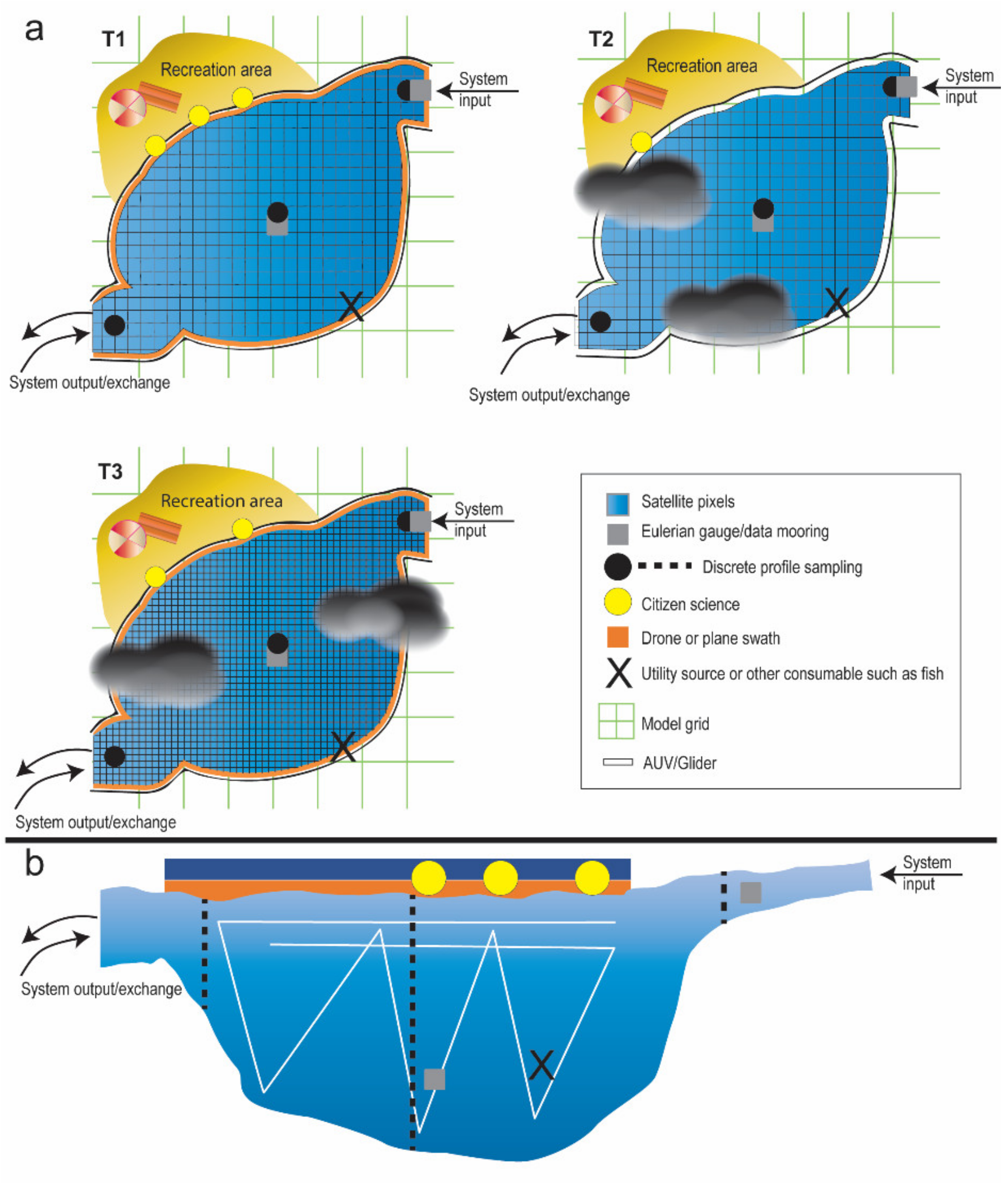
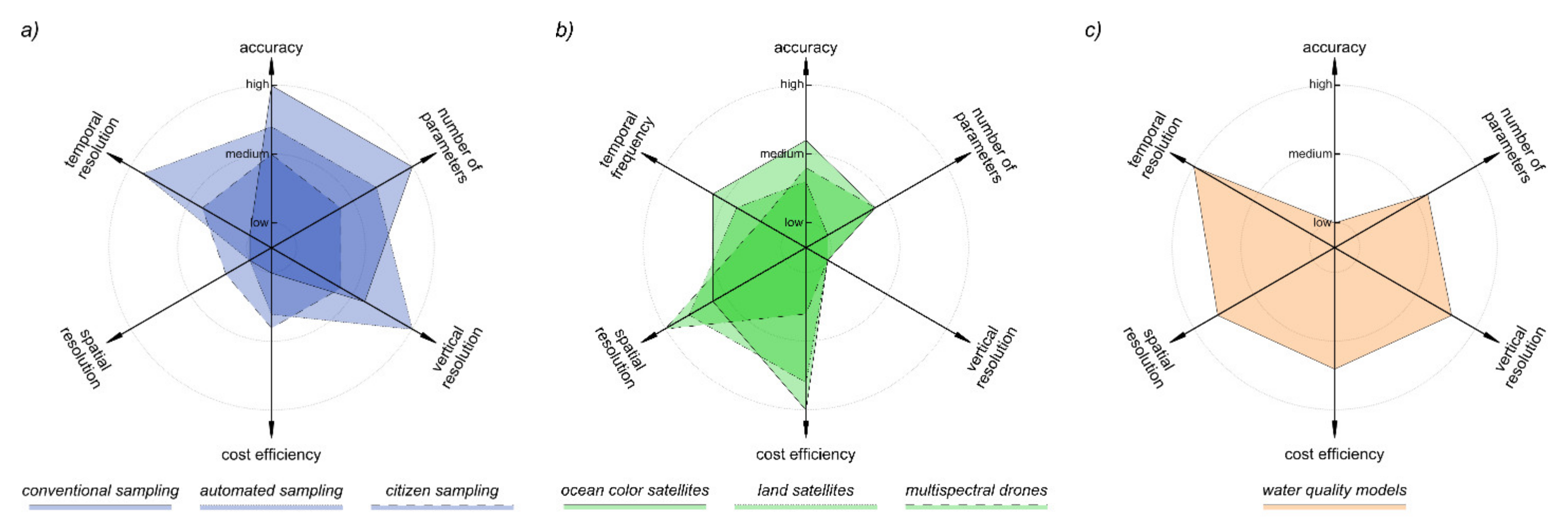
3. Overview of Observational Methods and Platforms
3.1. Discrete Sampling
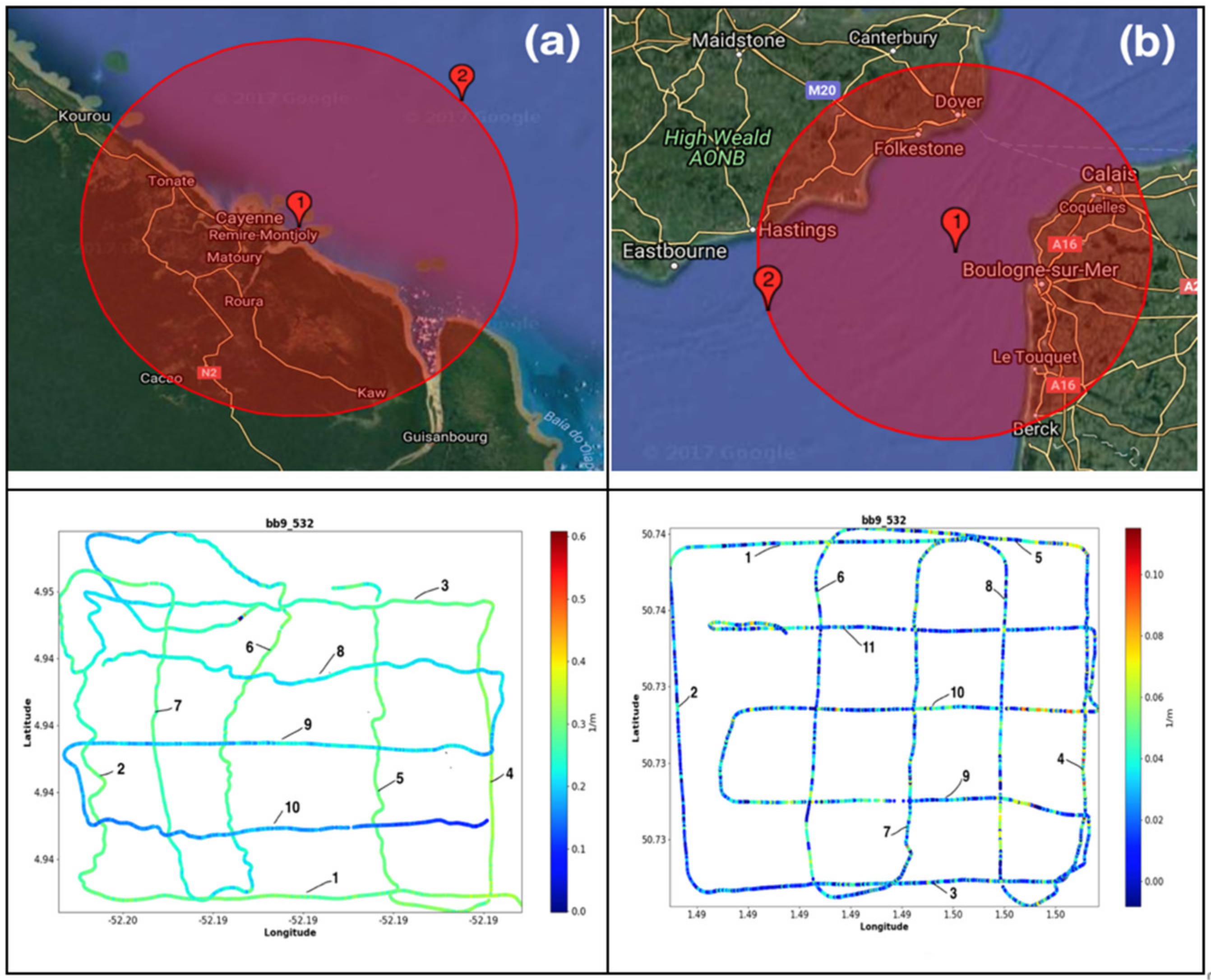
3.2. Continous Sampling
3.3. Remote Sensing
3.3.1. Passive Remote Sensing
3.3.2. Active Remote Sensing
3.3.3. Drone and Aircraft Systems
3.4. Volunteer Monitoring
3.5. Models
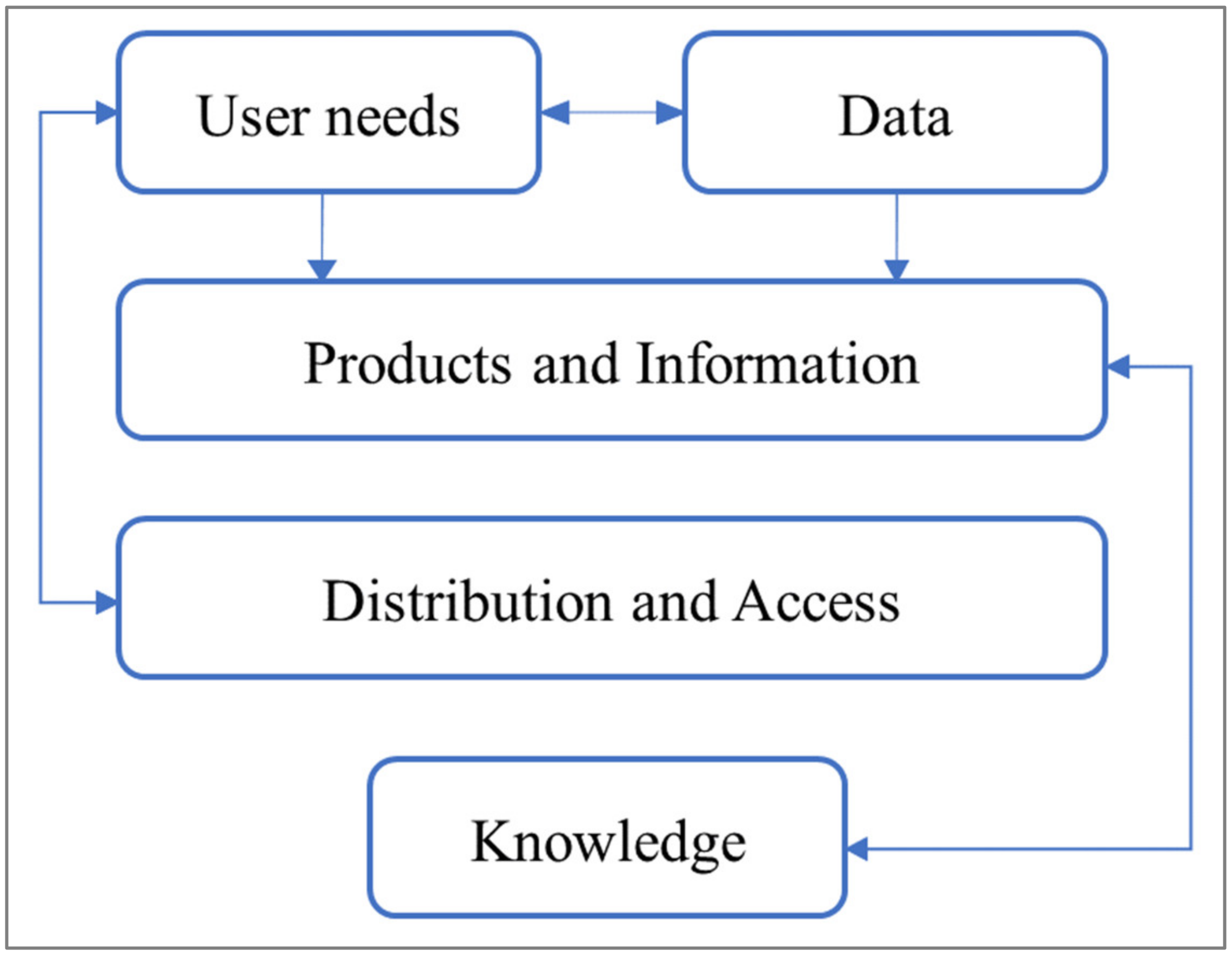
4. Data Integration
Integration Framework
5. Summary
Author Contributions
Funding
Institutional Review Board Statement
Informed Consent Statement
Data Availability Statement
Acknowledgments
Conflicts of Interest
References
- Neeley, A.R.; Mannino, A.; Reynolds, R.A.; Roesler, C.; Rottgers, R.; Stramski, D.; Twardowski, M.; Zaneveld, J.R.V. Ocean Optics & Biogeochemistry Protocols for Satellite Ocean Colour Sensor Validation; IOCCG: Dartmouth, NS, Canada, 2018. [Google Scholar]
- Brown, C.M.; Lund, J.R.; Cai, X.; Reed, P.M.; Zagona, E.A.; Ostfeld, A.; Hall, J.; Characklis, G.W.; Yu, W.; Brekke, L. The Future of Water Resources Systems Analysis: Toward a Scientific Framework for Sustainable Water Management. Water Resour. Res. 2015, 51, 6110–6124. [Google Scholar]
- Schaeffer, B.A.; Schaeffer, K.G.; Keith, D.; Lunetta, R.S.; Conmy, R.; Gould, R.W. Barriers to Adopting Satellite Remote Sensing for Water Quality Management. Int. J. Remote. Sens. 2013, 34, 7534–7544. [Google Scholar] [CrossRef]
- Agrawala, S.; Broad, K.; Guston, D.H. Integrating Climate Forecasts and Societal Decision Making: Challenges to an Emergent Boundary Organization. Sci. Technol. Hum. Values 2001, 26, 454–477. [Google Scholar] [CrossRef]
- Dilling, L.; Lemos, M.C. Creating Usable Science: Opportunities and Constraints for Climate Knowledge Use and Their Implications for Science Policy. Glob. Environ. Chang. 2011, 21, 680–689. [Google Scholar] [CrossRef]
- Lemos, M.C.; Morehouse, B.J. The Co-Production of Science and Policy in Integrated Climate Assessments. Glob. Environ. Chang. 2005, 15, 57–68. [Google Scholar] [CrossRef]
- Dietze, M.C. Ecological Forecasting; Princeton University Press: Princeton, NJ, USA, 2017. [Google Scholar]
- Lofton, M.E.; Leach, T.H.; Beisner, B.E.; Carey, C.C. Relative Importance of Top-Down vs Bottom-up Control of Lake Phytoplankton Vertical Distributions Varies among Fluorescence-Based Spectral Groups. Limnol. Oceanogr. 2020, 65, 2485–2501. [Google Scholar] [CrossRef]
- Thomas, R.N.; Paluszny, A.; Zimmerman, R.W. Permeability of Three-Dimensional Numerically Grown Geomechanical Discrete Fracture Networks with Evolving Geometry and Mechanical Apertures. J. Geophys. Res. Solid Earth 2020, 125, e2019JB018899. [Google Scholar] [CrossRef]
- Wilkinson, M.D.; Dumontier, M.; Aalbersberg, I.J.; Appleton, G.; Axton, M.; Baak, A.; Blomberg, N.; Boiten, J.W.; da Silva Santos, L.B.; Bourne, P.E.; et al. Comment: The Fair Guiding Principles for Scientific Data Management and Stewardship. Sci. Data 2016, 3, 160018. [Google Scholar] [CrossRef] [PubMed] [Green Version]
- Scheffer, M.; Bascompte, J.; Brock, W.A.; Brovkin, V.; Carpenter, S.R.; Dakos, V.; Held, H.; van Nes, E.; Rietkerk, M.; Sugihara, G. Early-Warning Signals for Critical Transitions. Nature 2009, 461, 53–59. [Google Scholar] [CrossRef] [PubMed]
- Kirschke, S.; Avellán, T.; Bärlund, I.; Bogardi, J.J.; Carvalho, L.; Chapman, D.; Dickens, C.W.S.; Irvine, K.; Lee, S.; Mehner, T. Capacity Challenges in Water Quality Monitoring: Understanding the Role of Human Development. Environ. Monit. Assess. 2020, 192, 1–16. [Google Scholar] [CrossRef] [Green Version]
- Kaku, K. Satellite Remote Sensing for Disaster Management Support: A Holistic and Staged Approach Based on Case Studies in Sentinel Asia. Int. J. Disaster Risk Reduct. 2019, 33, 417–432. [Google Scholar] [CrossRef]
- Bojinski, S.; Verstraete, M.; Peterson, T.C.; Richter, C.; Simmons, A.; Zemp, M. The Concept of Essential Climate Variables in Support of Climate Research, Applications, and Policy. Bull. Am. Meteorol. Soc. 2014, 95, 1431–1443. [Google Scholar] [CrossRef]
- Lawford, R.; Strauch, A.; Toll, D.; Fekete, B.; Cripe, D. Earth observations for global water security. Curr. Opin. Environ. Sustain. 2013, 5, 633–643. [Google Scholar] [CrossRef] [Green Version]
- Pereira, H.M.; Ferrier, S.; Walters, M.; Geller, G.N.; Jongman, R.H.G.; Scholes, R.J.; Bruford, M.W.; Brummitt, N.; Butchart, S.H.M.; Cardoso, A.C.; et al. Essential Biodiversity Variables. Science 2013, 339, 277–278. [Google Scholar] [CrossRef] [Green Version]
- Dickey, T.; Lewis, M.; Chang, G. Optical Oceanography: Recent Advances and Future Directions Using Global Remote Sensing and in Situ Observations. Rev. Geophys. 2006, 44. [Google Scholar] [CrossRef] [Green Version]
- Boss, E.E.D.; Freeman, S.; Fry, E.; Mueller, J.; Pegau, S.; Rick, A.R.; Roesler, C.; Rottgers, R.; Stramski, D.; Twardowski, M.; et al. Inherent Optical Property Measurements and Protocols: Absorption Coefficient. In Ioccg Protocol Series: Ocean Optics & Biogeochemistry Protocols for Satellite Ocean Colour Sensor Validation; Neeley, A., Mannino, A., Eds.; IOCCG: Dartmouth, NS, Canada, 2018; p. 86. [Google Scholar]
- Boss, E.N.H.; Steven, A.G.; Balch, B.; Chase, A.; Dall’Olmo, G.; Freeman, S.; Liu, Y.; Loftin, J.; Neary, W. Inherent Optical Property Measurements and Protocols: Best Practices for the Collection and Processing of Ship-Based Underway Flow-through Optical Data. In Ioccg Ocean Optics and Biogeochemistry Protocols for Satellite Ocean Colour Sensor Validation; IOCCG: Dartmouth, NS, Canada, 2019. [Google Scholar]
- Neeley, A.; Cetinić, I. Beam Transmission and Attenuation Coefficients: Instruments, Characterization, Field Measurements and Data Analysis Protocols. In Ocean Optics and Biogeochemistry Protocols for Satellite Ocean Colour Sensor Validation; IOCCG: Dartmouth, NS, Canada, 2019. [Google Scholar]
- Ruddick, K.G.; Voss, K.; Banks, A.C.; Boss, E.; Castagna, A.; Frouin, R.; Hieronymi, M.; Jamet, C.; Johnson, B.C.; Kuusk, J. A Review of Protocols for Fiducial Reference Measurements of Downwelling Irradiance for the Validation of Satellite Remote Sensing Data over Water. Remote Sens. 2019, 11, 1742. [Google Scholar] [CrossRef] [Green Version]
- Ruddick, K.G.; Voss, K.; Boss, E.; Castagna, A.; Frouin, R.; Gilerson, A.; Hieronymi, M.; Johnson, B.C.; Kuusk, J.; Lee, Z. A Review of Protocols for Fiducial Reference Measurements of Water-Leaving Radiance for Validation of Satellite Remote-Sensing Data over Water. Remote Sens. 2019, 11, 2198. [Google Scholar] [CrossRef] [Green Version]
- Tilstone, G.; Dall’Olmo, G.; Hieronymi, M.; Ruddick, K.; Beck, M.; Ligi, M.; Costa, M.; D’alimonte, D.; Vellucci, V.; Vansteenwegen, D. Field Intercomparison of Radiometer Measurements for Ocean Colour Validation. Remote Sens. 2020, 12, 1587. [Google Scholar] [CrossRef]
- Vabson, V.; Kuusk, J.; Ansko, I.; Vendt, R.; Alikas, K.; Ruddick, K.; Ansper, A.; Bresciani, M.; Burmester, H.; Costa, M. Laboratory Intercomparison of Radiometers Used for Satellite Validation in the 400–900 Nm Range. Remote Sens. 2019, 11, 1101. [Google Scholar] [CrossRef] [Green Version]
- Vabson, V.; Kuusk, J.; Ansko, I.; Vendt, R.; Alikas, K.; Ruddick, K.; Ansper, A.; Bresciani, M.; Burmester, H.; Costa, M.; et al. Field Intercomparison of Radiometers Used for Satellite Validation in the 400–900 Nm Range. Remote Sens. 2019, 11, 1129. [Google Scholar] [CrossRef] [Green Version]
- Zibordi, G.; Voss, K.J.; Johnson, B.C.; Mueller, J.L. IOCCG Ocean Optics and Biogeochemistry Protocols for Satellite Ocean Colour Sensor Validation; IOCCG Protocols Series 3; IOCCG: Dartmouth, NS, Canada, 2019. [Google Scholar]
- Rose, K.C.; Weathers, K.C.; Hetherington, A.L.; Hamilton, D.P. Insights from the Global Lake Ecological Observatory Network (Gleon). Inland Waters 2016, 6, 476–482. [Google Scholar] [CrossRef] [Green Version]
- Banks, A.C.; Vendt, R.; Alikas, K.; Bialek, A.; Kuusk, J.; Lerebourg, C.; Ruddick, K.; Tilstone, G.; Vabson, V.; Donlon, C. Fiducial Reference Measurements for Satellite Ocean Colour (Frm4soc). Remote Sens. 2020, 12, 1322. [Google Scholar] [CrossRef] [Green Version]
- Slade, W.H.; Boss, E.; Dall’Olmo, G.; Langner, M.R.; Loftin, J.; Behrenfeld, M.J.; Roesler, C.; Westberry, T.K. Underway and Moored Methods for Improving Accuracy in Measurement of Spectral Particulate Absorption and Attenuation. J. Atmos. Ocean. Technol. 2010, 27, 1733–1746. [Google Scholar] [CrossRef]
- Werdell, P.J.; Proctor, C.W.; Boss, E.; Leeuw, T.; Ouhssain, M. Underway Sampling of Marine Inherent Optical Properties on the Tara Oceans Expedition as a Novel Resource for Ocean Color Satellite Data Product Validation. Methods Oceanogr. 2013, 7, 40–51. [Google Scholar] [CrossRef]
- Jayne, S.R.; Roemmich, D.; Zilberman, N.; Riser, S.C.; Johnson, K.S.; Johnson, G.C.; Piotrowicz, S.R. The Argo Program: Present and Future. Oceanography 2017, 30, 18–28. [Google Scholar] [CrossRef]
- Antoine, D.; Guevel, P.; Desté, J.; Bécu, G.; Louis, F.; Scott, A.J.; Bardey, P. The Boussole Buoy—A New Transparent-to-Swell Taut Mooring Dedicated to Marine Optics: Design, Tests, and Performance at Sea. J. Atmos. Ocean. Technol. 2008, 25, 968–989. [Google Scholar] [CrossRef]
- Claustre, H.; Johnson, K.S.; Takeshita, Y. Observing the Global Ocean with Biogeochemical-Argo. Annu. Rev. Mar. Sci. 2020, 12, 23–48. [Google Scholar] [CrossRef]
- Testor, P.; de Young, B.; Rudnick, D.L.; Glenn, S.; Hayes, D.; Lee, C.M.; Pattiaratchi, C.; Hill, K.; Heslop, E.; Turpin, V. Oceangliders: A Component of the Integrated Goos. Front. Mar. Sci. 2019, 6, 422. [Google Scholar] [CrossRef] [Green Version]
- Moses, W.J.; Ackleson, S.G.; Hair, J.W.; Hostetler, C.A.; Miller, W.D. Spatial Scales of Optical Variability in the Coastal Ocean: Implications for Remote Sensing and in Situ Sampling. J. Geophys. Res. Ocean. 2016, 121, 4194–4208. [Google Scholar] [CrossRef] [Green Version]
- Zibordi, G.; Mélin, F.; Berthon, J.; Holben, B.; Slutsker, I.; Giles, D.; D’Alimonte, D.; Vandemark, D.; Feng, H.; Schuster, G. Aeronet-Oc: A Network for the Validation of Ocean Color Primary Products. J. Atmos. Ocean. Technol. 2009, 26, 1634–1651. [Google Scholar] [CrossRef]
- Boucher, J.; Weathers, K.C.; Norouzi, H.; Steele, B. Assessing the Effectiveness of Landsat 8 Chlorophyll a Retrieval Algorithms for Regional Freshwater Monitoring. Ecol. Appl. 2018, 28, 1044–1054. [Google Scholar] [CrossRef] [PubMed] [Green Version]
- Harvey, E.T.; Kratzer, S.; Philipson, P. Satellite-Based Water Quality Monitoring for Improved Spatial and Temporal Retrieval of Chlorophyll-a in Coastal Waters. Remote Sens. Environ. 2015, 158, 417–430. [Google Scholar] [CrossRef]
- Palmer, S.C.J.; Kutser, T.; Hunter, P.D. Remote Sensing of Inland Waters: Challenges, Progress and Future Directions; Elsevier: Amsterdam, The Netherlands, 2015. [Google Scholar]
- Tyler, A.N.; Hunter, P.D.; Spyrakos, E.; Groom, S.; Constantinescu, A.M.; Kitchen, J. Developments in Earth Observation for the Assessment and Monitoring of Inland, Transitional, Coastal and Shelf-Sea Waters. Sci. Total Environ. 2016, 572, 1307–1321. [Google Scholar] [CrossRef] [PubMed] [Green Version]
- Balasubramanian, S.V.; Pahlevan, N.; Smith, B.; Binding, C.; Schalles, J.; Loisel, H.; Gurlin, D.; Greb, S.; Alikas, K.; Randla, M. Robust Algorithm for Estimating Total Suspended Solids (Tss) in Inland and Nearshore Coastal Waters. Remote Sens. Environ. 2020, 246, 111768. [Google Scholar] [CrossRef]
- Goyens, C.; Jamet, C.; Schroeder, T. Evaluation of Four Atmospheric Correction Algorithms for Modis-Aqua Images over Contrasted Coastal Waters. Remote Sens. Environ. 2013, 131, 63–75. [Google Scholar] [CrossRef]
- Matthews, M.W. A Current Review of Empirical Procedures of Remote Sensing in Inland and near-Coastal Transitional Waters. Int. J. Remote Sens. 2011, 32, 6855–6899. [Google Scholar] [CrossRef]
- Mograne, M.A.; Jamet, C.; Loisel, H.; Vantrepotte, V.; Mériaux, X.; Cauvin, A. Evaluation of Five Atmospheric Correction Algorithms over French Optically-Complex Waters for the Sentinel-3a Olci Ocean Color Sensor. Remote Sens. 2019, 11, 668. [Google Scholar] [CrossRef] [Green Version]
- Odermatt, D.; Gitelson, A.; Brando, V.E.; Schaepman, M. Review of Constituent Retrieval in Optically Deep and Complex Waters from Satellite Imagery. Remote Sens. Environ. 2012, 118, 116–126. [Google Scholar] [CrossRef] [Green Version]
- Pahlevan, N.; Balasubramanian, S.V.; Sarkar, S.; Franz, B.A. Toward Long-Term Aquatic Science Products from Heritage Landsat Missions. Remote Sens. 2018, 10, 1337. [Google Scholar] [CrossRef] [Green Version]
- Pahlevan, N.; Chittimalli, S.K.; Balasubramanian, S.V.; Vellucci, V. Sentinel-2/Landsat-8 Product Consistency and Implications for Monitoring Aquatic Systems. Remote Sens. Environ. 2019, 220, 19–29. [Google Scholar] [CrossRef]
- Pahlevan, N.; Smith, B.; Schalles, J.; Binding, C.; Cao, Z.; Ma, R.; Alikas, K.; Kangro, K.; Gurlin, D.; Hà, N. Seamless Retrievals of Chlorophyll-a from Sentinel-2 (Msi) and Sentinel-3 (Olci) in Inland and Coastal Waters: A Machine-Learning Approach. Remote Sens. Environ. 2020, 240, 111604. [Google Scholar] [CrossRef]
- Tzortziou, M.; Parker, O.; Lamb, B.; Herman, J.; Lamsal, L.; Stauffer, R.; Abuhassan, N. Atmospheric Trace Gas (No2 and O3) Variability in South Korean Coastal Waters, and Implications for Remote Sensing of Coastal Ocean Color Dynamics. Remote Sens. 2018, 10, 1587. [Google Scholar] [CrossRef] [Green Version]
- Schollaert, U.S.; Kim, G.E.; Mannino, A.; Werdell, P.J.; Tzortziou, M. Developing a Community of Practice for Applied Uses of Future Pace Data to Address Marine Food Security Challenges. Front. Earth Sci. 2019, 7, 283. [Google Scholar] [CrossRef] [Green Version]
- Werdell, P.J.; McKinna, L.I.; Boss, E.; Ackleson, S.G.; Craig, S.E.; Gregg, W.W.; Lee, Z.; Maritorena, S.; Roesler, C.S.; Rousseaux, C.S.; et al. An Overview of Approaches and Challenges for Retrieving Marine Inherent Optical Properties from Ocean Color Remote Sensing. Prog. Oceanogr. 2018, 160, 186–212. [Google Scholar] [CrossRef] [PubMed]
- Vanhellemont, Q.; Ruddick, K. Atmospheric Correction of Metre-Scale Optical Satellite Data for Inland and Coastal Water Applications. Remote Sens. Environ. 2018, 216, 586–597. [Google Scholar] [CrossRef]
- Helder, D.; Markham, B.; Morfitt, R.; Storey, J.; Barsi, J.; Gascon, F.; Clerc, S.; LaFrance, B.; Masek, J.; Roy, D.; et al. Observations and Recommendations for the Calibration of Landsat 8 Oli and Sentinel 2 Msi for Improved Data Interoperability. Remote Sens. 2018, 10, 1340. [Google Scholar] [CrossRef] [Green Version]
- Antonini, K.; Langer, M.; Farid, A.; Walter, U. Sweet Cubesat–Water Detection and Water Quality Monitoring for the 21st Century. Acta Astronaut. 2017, 140, 10–17. [Google Scholar] [CrossRef]
- Alvera-Azcárate, A.; Vanhellemont, Q.; Ruddick, K.; Barth, A.; Beckers, J.M. Analysis of High Frequency Geostationary Ocean Colour Data Using Dineof. Estuar. Coast. Shelf Sci. 2015, 159, 28–36. [Google Scholar] [CrossRef] [Green Version]
- Choi, J.-K.; Min, J.-E.; Noh, J.H.; Han, T.-H.; Yoon, S.; Park, Y.J.; Moon, J.-E.; Ahn, J.-H.; Ahn, S.M.; Park, J.-H. Harmful algal bloom (HAB) in the East Sea identified by the Geostationary Ocean Color Imager (GOCI). Harmful Algae 2014, 39, 295–302. [Google Scholar] [CrossRef]
- Choi, J.-K.; Park, Y.J.; Lee, B.R.; Eom, J.; Moon, J.; Ryu, J. Application of the Geostationary Ocean Color Imager (Goci) to Mapping the Temporal Dynamics of Coastal Water Turbidity. Remote Sens. Environ. 2014, 146, 24–35. [Google Scholar] [CrossRef]
- Ody, A.; Doxaran, D.; Vanhellemont, Q.; Nechad, B.; Novoa, S.; Many, G.; Bourrin, F.; Verney, R.; Pairaud, I.; Gentili, B. Potential of High Spatial and Temporal Ocean Color Satellite Data to Study the Dynamics of Suspended Particles in a Micro-Tidal River Plume. Remote Sens. 2016, 8, p245. [Google Scholar] [CrossRef] [Green Version]
- Muller-Karger, F.E.; Hestir, E.; Ade, C.; Turpie, K.; Roberts, D.A.; Siegel, D.; Miller, R.J.; Humm, D.; Izenberg, N.; Keller, M.; et al. Satellite Sensor Requirements for Monitoring Essential Biodiversity Variables of Coastal Ecosystems. Ecol. Appl. 2018, 28, 749–760. [Google Scholar] [CrossRef] [PubMed]
- Macauley, M.K. The Value of Information: A Background Paper on Measuring the Contribution of Space-Derived Earth Science Data to National Resource Management; Resources for the Future: Washington, DC, USA, 2005. [Google Scholar]
- Sagoff, M. On the Economic Value of Ecosystem Services. Environ. Values 2008, 17, 239–257. [Google Scholar] [CrossRef] [Green Version]
- Gholizadeh, M.H.; Melesse, A.M.; Reddi, L. A Comprehensive Review on Water Quality Parameters Estimation Using Remote Sensing Techniques. Sensors 2016, 16, 1298. [Google Scholar] [CrossRef] [PubMed] [Green Version]
- Loisel, H.; Vantrepotte, V.; Jamet, C.; Dat, D.N. Challenges and New Advances in Ocean Color Remote Sensing of Coastal Waters. Top. Oceanogr. 2013, 1–38. [Google Scholar]
- Mouw, C.B.; Greb, S.; Aurin, D.; DiGiacomo, P.M.; Lee, Z.; Twardowski, M.; Binding, C.; Hu, C.; Ma, R.; Moore, T. Aquatic Color Radiometry Remote Sensing of Coastal and Inland Waters: Challenges and Recommendations for Future Satellite Missions. Remote Sens. Environ. 2015, 160, 15–30. [Google Scholar] [CrossRef]
- Zheng, G.; DiGiacomo, P.M. Uncertainties and Applications of Satellite-Derived Coastal Water Quality Products. Prog. Oceanogr. 2017, 159, 45–72. [Google Scholar] [CrossRef]
- Diehl, S.; Berger, S.; Ptacnik, R.; Wild, A. Phytoplankton, Light, and Nutrients in a Gradient of Mixing Depths: Field Experiments. Ecology 2002, 83, 399–411. [Google Scholar] [CrossRef]
- Dörnhöfer, K.; Oppelt, N. Remote Sensing for Lake Research and Monitoring–Recent Advances. Ecol. Indic. 2016, 64, 105–122. [Google Scholar] [CrossRef]
- Bresciani, M.; Adamo, M.; de Carolis, G.; Matta, E.; Pasquariello, G.; Vaičiūtė, D.; Giardino, C. Monitoring Blooms and Surface Accumulation of Cyanobacteria in the Curonian Lagoon by Combining Meris and Asar Data. Remote Sens. Environ. 2014, 146, 124–135. [Google Scholar] [CrossRef]
- Lin, I.I.; Wen, L.S.; Liu, K.K.; Tsai, W.T.; Liu, A.K. Evidence and Quantification of the Correlation between Radar Backscatter and Ocean Colour Supported by Simultaneously Acquired in Situ Sea Truth. Geophys. Res. Lett. 2002, 29, 102. [Google Scholar] [CrossRef] [Green Version]
- Churnside, J.H. Review of Profiling Oceanographic Lidar. Opt. Eng. 2013, 53, 051405. [Google Scholar] [CrossRef] [Green Version]
- Churnside, J.H.; Shaw, J.A. Lidar Remote Sensing of the Aquatic Environment. Appl. Opt. 2020, 59, C92–C99. [Google Scholar] [CrossRef]
- Hostetler, C.A.; Behrenfeld, M.J.; Hu, Y.; Hair, J.W.; Schulien, A.J. Spaceborne Lidar in the Study of Marine Systems. Annu. Rev. Mar. Sci. 2018, 10, 121–147. [Google Scholar] [CrossRef] [PubMed] [Green Version]
- Jamet, C.; Ibrahim, A.; Ahmad, Z.; Angelini, F.; Babin, M.; Behrenfeld, J.M.; Boss, E.; Cairns, B.; Churnside, J.; Chowdhary, J. Going Beyond Standard Ocean Color Observations: Lidar and Polarimetry. Front. Mar. Sci. 2019, 6, 251. [Google Scholar] [CrossRef]
- Churnside, J.H.; Demer, D.A.; Mahmoudi, B. A Comparison of Lidar and Echosounder Measurements of Fish Schools in the Gulf of Mexico. ICES J. Mar. Sci. 2003, 60, 147–154. [Google Scholar] [CrossRef]
- Churnside, J.H.; Donaghay, P.L. Thin Scattering Layers Observed by Airborne Lidar. ICES J. Mar. Sci. 2009, 66, 778–789. [Google Scholar] [CrossRef]
- Behrenfeld, M.J.; Hu, Y.; Hostetler, C.A.; Dall’Olmo, G.; Rodier, S.D.; Hair, J.W.; Trepte, C.R. Space-Based Lidar Measurements of Global Ocean Carbon Stocks. Geophys. Res. Lett. 2013, 40, 4355–4360. [Google Scholar] [CrossRef]
- Dionisi, D.; Brando, V.E.; Volpe, G.; Colella, S.; Santoleri, R. Seasonal Distributions of Ocean Particulate Optical Properties from Spaceborne Lidar Measurements in Mediterranean and Black Sea. Remote Sens. Environ. 2020, 247, 111889. [Google Scholar] [CrossRef]
- Lu, X.; Hu, Y.; Trepte, C.; Zeng, S.; Churnside, J.H. Ocean Subsurface Studies with the Calipso Spaceborne Lidar. J. Geophys. Res. Ocean. 2014, 119, 4305–4317. [Google Scholar] [CrossRef]
- Lu, X.; Hu, Y.; Yang, Y.; Bontempi, P.; Omar, A.; Baize, R. Antarctic Spring Ice-Edge Blooms Observed from Space by Icesat-2. Remote Sens. Environ. 2020, 245, 111827. [Google Scholar] [CrossRef]
- Tarpanelli, A.; Benveniste, J. Chapter Eleven—On the Potential of Altimetry and Optical Sensors for Monitoring and Forecasting River Discharge and Extreme Flood Events. In Extreme Hydroclimatic Events and Multivariate Hazards in a Changing Environment; Maggioni, V., Massari, C., Eds.; Elsevier: Amsterdam, The Netherlands, 2019. [Google Scholar]
- Fu, L.-L.; Cazenave, A. Satellite Altimetry and Earth Sciences: A Handbook of Techniques and Applications; Elsevier: Amsterdam, The Netherlands, 2000. [Google Scholar]
- Grgić, M.; Bašić, T. Radar Satellite Altimetry in Geodesy-Theory, Applications and Recent Developments. In Geodetic Sciences-Theory, Applications and Recent Developments; IntechOpen: London, UK, 2021. [Google Scholar]
- Ansper-Toomsalu, A.; Alikas, K.; Nielsen, K.; Tuvikene, L.; Kangro, K. Synergy between Satellite Altimetry and Optical Water Quality Data Towards Improved Estimation of Lakes Ecological Status. Remote Sens. 2021, 13, 770. [Google Scholar] [CrossRef]
- Tarpanelli, A.; Santi, E.; Tourian, M.J.; Filippucci, P.; Amarnath, G.; Brocca, L. Daily River Discharge Estimates by Merging Satellite Optical Sensors and Radar Altimetry through Artificial Neural Network. IEEE Trans. Geosci. Remote Sens. 2019, 57, 329–341. [Google Scholar] [CrossRef]
- Tourian, M.J.; Tarpanelli, A.; Elmi, O.; Qin, T.; Brocca, L.; Moramarco, T.; Sneeuw, N. Spatiotemporal Densification of River Water Level Time Series by Multimission Satellite Altimetry. Water Resour. Res. 2016, 52, 1140–1159. [Google Scholar] [CrossRef] [Green Version]
- De Keukelaere, L.; Sterckx, S.; Adriaensen, S.; Knaeps, E.; Reusen, I.; Giardino, C.; Bresciani, M.; Hunter, P.; Neil, C.; Van der Zande, D. Atmospheric Correction of Landsat-8/Oli and Sentinel-2/Msi Data Using Icor Algorithm: Validation for Coastal and Inland Waters. Eur. J. Remote Sens. 2018, 51, 525–542. [Google Scholar] [CrossRef] [Green Version]
- Koparan, C.; Koc, A.B.; Privette, C.V.; Sawyer, B.C. In Situ Water Quality Measurements Using an Unmanned Aerial Vehicle (Uav) System. Water 2018, 10, 264. [Google Scholar] [CrossRef] [Green Version]
- Su, T.-C.; Chou, H.-T. Application of Multispectral Sensors Carried on Unmanned Aerial Vehicle (UAV) to Trophic State Mapping of Small Reservoirs: A Case Study of Tain-Pu Reservoir in Kinmen, Taiwan. Remote Sens. 2015, 7, 10078–10097. [Google Scholar] [CrossRef] [Green Version]
- Aguirre-Gómez, R.; Salmerón-García, O.; Gómez-Rodríguez, G.; Peralta-Higuera, A. Use of Unmanned Aerial Vehicles and Remote Sensors in Urban Lakes Studies in Mexico. Int. J. Remote Sens. 2017, 38, 2771–2779. [Google Scholar] [CrossRef]
- Van der Merwe, D.; Price, K.P. Harmful Algal Bloom Characterization at Ultra-High Spatial and Temporal Resolution Using Small Unmanned Aircraft Systems. Toxins 2015, 7, 1065–1078. [Google Scholar] [CrossRef] [Green Version]
- Flynn, K.F.; Chapra, S.C. Remote Sensing of Submerged Aquatic Vegetation in a Shallow Non-Turbid River Using an Unmanned Aerial Vehicle. Remote Sens. 2014, 6, 12815–12836. [Google Scholar] [CrossRef] [Green Version]
- Husson, E.; Hagner, O.; Ecke, F. Unmanned Aircraft Systems Help to Map Aquatic Vegetation. Appl. Veg. Sci. 2014, 17, 567–577. [Google Scholar] [CrossRef]
- Shang, S.; Lee, Z.; Lin, G.; Hu, C.; Shi, L.; Zhang, Y.; Li, X.; Wu, J.; Yan, J. Sensing an intense phytoplankton bloom in the western Taiwan Strait from radiometric measurements on a UAV. Remote. Sens. Environ. 2017, 198, 85–94. [Google Scholar] [CrossRef]
- Sáenz, N.A.; Paez, D.E.; Arango, C. Local Algorithm for Monitoring Total Suspended Sediments in Micro-Watersheds Usin Drones and Remote Sensing Applications. Case Study: Teusacá River, La Calera, Colombia. Int. Arch. Photogramm. Remote. Sens. Spat. Inf. Sci. 2015, 40. [Google Scholar] [CrossRef] [Green Version]
- De Keukelaere, L.; Moelans, R.; Strackx, G.; Knaeps, E.; Lemey, E. Mapping Water Quality with Drones: Test Case in Texel. Terra et Aqua 2019, 157, 6–16. [Google Scholar]
- Ore, J.-P.; Elbaum, S.; Burgin, A.; Detweiler, C. Autonomous Aerial Water Sampling. J. Field Robot. 2015, 32, 1095–1113. [Google Scholar] [CrossRef] [Green Version]
- Gentemann, C.L.; Scott, J.P.; Mazzini, P.L.F.; Pianca, C.; Akella, S.; Minnett, P.J.; Cornillon, P.; Fox-Kemper, B.; Cetinić, I.; Chin, T.M. Saildrone: Adaptively Sampling the Marine Environment. Bull. Am. Meteorol. Soc. 2020, 101, E744–E762. [Google Scholar] [CrossRef] [Green Version]
- Meinig, C.; Burger, E.F.; Cohen, N.; Cokelet, E.D.; Cronin, M.F.; Cross, J.N.; de Halleux, S.; Jenkins, R.; Jessup, A.T.; Mordy, C.W. Public–Private Partnerships to Advance Regional Ocean-Observing Capabilities: A Saildrone and Noaa-Pmel Case Study and Future Considerations to Expand to Global Scale Observing. Front. Mar. Sci. 2019, 6, 448. [Google Scholar] [CrossRef] [Green Version]
- Petrie, G. Commercial Operation of Lightweight. GEO Inform. 2013, 16, 28. [Google Scholar]
- Tweddle, J.C.; Robinson, L.D.; Pocock, M.J.O.; Roy, H.E. Guide to Citizen Science: Developing, Implementing and Evaluating Citizen Science to Study Biodiversity and the Environment in the UK. NERC/Centre for Ecology & Hydrology: Lancaster, UK, 2012. [Google Scholar]
- Pocock, M.J.O.; Roy, H.E.; August, T.; Kuria, A.; Barasa, F.; Bett, J.; Githiru, M.; Kairo, J.; Kimani, J.; Kinuthia, W. Developing the Global Potential of Citizen Science: Assessing Opportunities That Benefit People, Society and the Environment in East Africa. J. Appl. Ecol. 2019, 56, 274–281. [Google Scholar] [CrossRef]
- Malthus, T.J.; Ohmsen, R.; Woerd, H.J. An Evaluation of Citizen Science Smartphone Apps for Inland Water Quality Assessment. Remote Sens. 2020, 12, 1578. [Google Scholar] [CrossRef]
- Blaney, R.J.P.; Jones, G.; Philippe, A.; Pocock, M. Citizen Science and Environmental Monitoring: Towards a Methodology for Evaluating Opportunities, Costs and Benefits. In Final Report on behalf of UKEOF; UKEOF: Lancaster, UK, 2016. [Google Scholar]
- Hadj-Hammou, J.; Loiselle, S.; Ophof, D.; Thornhill, I. Getting the Full Picture: Assessing the Complementarity of Citizen Science and Agency Monitoring Data. PLoS ONE 2017, 12, e0188507. [Google Scholar] [CrossRef] [Green Version]
- Crooke, B.L.; McKinna, I.W.; Cetinić, I. From Toes to Top-of-Atmosphere: Fowler’s Sneaker Depth Index of Water Clarity for the Chesapeake Bay. Opt. Express 2017, 25, A361–A374. [Google Scholar] [CrossRef]
- Leeuw, T.; Boss, E. The Hydrocolor App: Above Water Measurements of Remote Sensing Reflectance and Turbidity Using a Smartphone Camera. Sensors 2018, 18, 256. [Google Scholar] [CrossRef] [PubMed] [Green Version]
- Hamilton, S.H.; Joseph, S.E.; Guillaume, H.A.; Jakeman, A.J.; Suzanne, A.P. Integrated Assessment and Modelling: Overview and Synthesis of Salient Dimensions. Environ. Model. Softw. 2015, 64, 215–229. [Google Scholar] [CrossRef]
- Hutter, K.; Johnk, K. Continuum Methods of Physical Modelling: Mechanics of Continua, Dimensional Analysis, Turbulance; Springer: New York, NY, USA, 2014. [Google Scholar]
- Stepanenko, V.M.; Goyette, S.; Martynov, A.; Perroud, M.; Fang, X.; Mironov, D. First Steps of a Lake Model Intercomparison Project: Lakemip. Boreal Environ. Res. 2010, 15, 191–202. [Google Scholar]
- Gaudard, A.; Vinnå, L.R.; Bärenbold, F.; Schmid, M.; Bouffard, D. Toward an Open Access to High-Frequency Lake Modeling and Statistics Data for Scientists and Practitioners–the Case of Swiss Lakes Using Simstrat V2.1. Geosci. Model Dev. 2019, 12, 3955–3974. [Google Scholar] [CrossRef] [Green Version]
- Woolway, R.I.; Merchant, C.J. Worldwide Alteration of Lake Mixing Regimes in Response to Climate Change. Nat. Geosci. 2019, 12, 271–276. [Google Scholar] [CrossRef]
- Frassl, M.A.; Abell, J.M.; Botelho, D.A.; Cinque, K.; Gibbes, B.R.; Jöhnk, K.D.; Muraoka, K.; Robson, B.J.; Wolski, M.; Xiao, M. A Short Review of Contemporary Developments in Aquatic Ecosystem Modelling of Lakes and Reservoirs. Environ. Model. Softw. 2019, 117, 181–187. [Google Scholar] [CrossRef]
- Janssen, A.B.G.; Arhonditsis, G.B.; Beusen, A.; Bolding, K.; Bruce, L.; Bruggeman, J.; Couture, R.; Downing, A.S.; Elliott, J.A.; Marieke, F. Exploring, Exploiting and Evolving Diversity of Aquatic Ecosystem Models: A Community Perspective. Aquat. Ecol. 2015, 49, 513–548. [Google Scholar] [CrossRef] [Green Version]
- Mieleitner, J.; Reichert, P. Modelling Functional Groups of Phytoplankton in Three Lakes of Different Trophic State. Ecol. Model. 2008, 211, 279–291. [Google Scholar] [CrossRef]
- Bouffard, D.; Kiefer, I.; Wüest, A.; Wunderle, S.; Odermatt, D. Are Surface Temperature and Chlorophyll in a Large Deep Lake Related? An Analysis Based on Satellite Observations in Synergy with Hydrodynamic Modelling and in-Situ Data. Remote Sens. Environ. 2018, 209, 510–523. [Google Scholar] [CrossRef] [Green Version]
- Nouchi, V.; Kutser, T.; Wüest, A.; Müller, B.; Odermatt, D.; Baracchini, T.; Bouffard, D. Resolving Biogeochemical Processes in Lakes Using Remote Sensing. Aquat. Sci. 2019, 81, 27. [Google Scholar] [CrossRef] [Green Version]
- Soulignac, F.; Danis, P.; Bouffard, D.; Chanudet, V.; Dambrine, E.; Guénand, Y.; Harmel, T.; Ibelings, B.W.; Trevisan, D.; Uittenbogaard, R. Using 3d Modeling and Remote Sensing Capabilities for a Better Understanding of Spatio-Temporal Heterogeneities of Phytoplankton Abundance in Large Lakes. J. Great Lakes Res. 2018, 44, 756–764. [Google Scholar] [CrossRef] [Green Version]
- Pahlevan, N.; Garrett, A.J.; Gerace, A.D.; Schott, J.R. Integrating Landsat 7 Imagery with Physics-Based Models for Quantitative Mapping of Coastal Waters near River Discharges. Photogramm. Eng. Remote Sens. (PE&RS) 2012, 78, 11. [Google Scholar]
- IOCCG. Synergy between Ocean Colour and Biogeochemical/Ecosystem Models; Dartmouth, S.D., Ed.; IOCCG: Dartmouth, NS, Canada, 2020. [Google Scholar]
- Rose, K.C.; Winslow, L.A.; Read, J.S.; Hansen, G.J.A. Climate-Induced Warming of Lakes Can Be Either Amplified or Suppressed by Trends in Water Clarity. Limnol. Oceanogr. Lett. 2016, 1, 44–53. [Google Scholar] [CrossRef]
- Baracchini, T.; Chu, P.Y.; Šukys, J.; Lieberherr, G.; Wunderle, S.; Wüest, A.; Bouffard, D. Data Assimilation of in Situ and Satellite Remote Sensing Data to 3d Hydrodynamic Lake Models: A Case Study Using Delft3d-Flow V4.03 and Openda V2.4. Geosci. Model Dev. 2020, 13, 1267–1284. [Google Scholar] [CrossRef] [Green Version]
- Baracchini, T.; Wüest, A.; Bouffard, D. Meteolakes: An Operational Online Three-Dimensional Forecasting Platform for Lake Hydrodynamics. Water Res. 2020, 172, 115529. [Google Scholar] [CrossRef]
- Clark, J.B.; Long, W.; Hood, R.R. A Comprehensive Estuarine Dissolved Organic Carbon Budget Using an Enhanced Biogeochemical Model. J. Geophys. Res. Biogeosci. 2020, 125, e2019JG005442. [Google Scholar] [CrossRef]
- Clark, J.B.; Long, W.; Tzortziou, M.; Neale, P.J.; Hood, R.R. Wind-Driven Dissolved Organic Matter Dynamics in a Chesapeake Bay Tidal Marsh-Estuary System. Estuaries Coasts 2018, 41, 708–723. [Google Scholar] [CrossRef]
- Clark, J.B.; Neale, P.; Tzortziou, M.; Cao, F.; Hood, R.R. A Mechanistic Model of Photochemical Transformation and Degradation of Colored Dissolved Organic Matter. Mar. Chem. 2019, 214, 103666. [Google Scholar] [CrossRef]
- Jones, E.M.; Baird, M.E.; Mongin, M.; Parslow, J.; Skerratt, J.; Lovell, J.; Margvelashvili, N.; Matear, R.J.; Wild-Allen, K.; Robson, B. Use of Remote-Sensing Reflectance to Constrain a Data Assimilating Marine Biogeochemical Model of the Great Barrier Reef. Biogeosciences 2016, 13, 6441–6469. [Google Scholar] [CrossRef] [Green Version]
- Kiefer, I.; Odermatt, D.; Anneville, O.; Wüest, A.; Bouffard, D. Application of Remote Sensing for the Optimization of in-Situ Sampling for Monitoring of Phytoplankton Abundance in a Large Lake. Sci. Total Environ. 2015, 527, 493–506. [Google Scholar] [CrossRef]
- Schaeffer, B.A.; Iiames, J.; Dwyer, J.; Urquhart, E.; Salls, W.; Rover, J.; Seegers, B. An Initial Validation of Landsat 5 and 7 Derived Surface Water Temperature for Us Lakes, Reservoirs, and Estuaries. Int. J. Remote Sens. 2018, 39, 7789–7805. [Google Scholar] [CrossRef]
- Otazu, X.; González-Audícana, M.; Fors, O.; Núñez, J. Introduction of Sensor Spectral Response into Image Fusion Methods. Application to Wavelet-Based Methods. IEEE Trans. Geosci. Remote Sens. 2005, 43, 2376–2385. [Google Scholar] [CrossRef] [Green Version]
- Zhu, X.X.; Grohnfeldt, C.; Bamler, R. Exploiting Joint Sparsity for Pansharpening: The J-Sparsefi Algorithm. IEEE Trans. Geosci. Remote Sens. 2016, 54, 2664–2681. [Google Scholar] [CrossRef] [Green Version]
- Aiazzi, B.; Alparone, L.; Baronti, S.; Garzelli, A.; Selva, M. Mtf-Tailored Multiscale Fusion of High-Resolution Ms and Pan Imagery. Photogramm. Eng. Remote Sens. 2006, 72, 591–596. [Google Scholar] [CrossRef]
- Pal, S.K.; Majumdar, T.J.; Bhattacharya, A.K. Ers-2 Sar and Irs-1c Liss Iii Data Fusion: A Pca Approach to Improve Remote Sensing Based Geological Interpretation. ISPRS J. Photogramm. Remote Sens. 2007, 61, 281–297. [Google Scholar] [CrossRef]
- Chang, N.-B.; Vannah, B.W.; Yang, Y.J.; Elovitz, M. Integrated Data Fusion and Mining Techniques for Monitoring Total Organic Carbon Concentrations in a Lake. Int. J. Remote Sens. 2014, 35, 1064–1093. [Google Scholar] [CrossRef]
- Dona, C.; Chang, N.; Caselles, V.; Sánchez, J.M.; Camacho, A.; Delegido, J.; Vannah, W.B. Integrated Satellite Data Fusion and Mining for Monitoring Lake Water Quality Status of the Albufera De Valencia in Spain. J. Environ. Manag. 2015, 151, 416–426. [Google Scholar] [CrossRef] [PubMed] [Green Version]
- Qin, B.; Li, W.; Zhu, G.; Zhang, Y.; Wu, T.; Gao, G. Cyanobacterial Bloom Management through Integrated Monitoring and Forecasting in Large Shallow Eutrophic Lake Taihu (China). J. Hazard. Mater. 2015, 287, 356–363. [Google Scholar] [CrossRef] [PubMed]
- Gao, F.; Hilker, T.; Zhu, X.; Anderson, M.; Masek, J.; Wang, P.; Yang, Y. Fusing Landsat and Modis Data for Vegetation Monitoring. IEEE Geosci. Remote Sens. Mag. 2015, 3, 47–60. [Google Scholar] [CrossRef]
- Liu, Y.; Gupta, H.V. Uncertainty in Hydrologic Modeling: Toward an Integrated Data Assimilation Framework. Water Resour. Res. 2007, 43. [Google Scholar] [CrossRef]
- Fiechter, J.; Broquet, G.; Moore, A.M.; Arango, H.G. A Data Assimilative, Coupled Physical–Biological Model for the Coastal Gulf of Alaska. Dyn. Atmos. Ocean. 2011, 52, 95–118. [Google Scholar] [CrossRef]
- El Serafy, G.Y.; Mynett, A.E. Improving the Operational Forecasting System of the Stratified Flow in Osaka Bay Using an Ensemble Kalman Filter-Based Steady State Kalman Filter. Water Resour. Res. 2008, 44. [Google Scholar] [CrossRef] [Green Version]
- Evensen, G. The Ensemble Kalman Filter: Theoretical Formulation and Practical Implementation. Ocean Dyn. 2003, 53, 343–367. [Google Scholar] [CrossRef]
- El Serafy, G.Y.; Marieke, A.; Blaas, E.M.; van Kessel, T.; Aguilar, S.G.; van der Woerd, H.J. Improving the Description of the Suspended Particulate Matter Concentrations in the Southern North Sea through Assimilating Remotely Sensed Data. Ocean Sci. J. 2011, 46, 179. [Google Scholar] [CrossRef] [Green Version]
- Karri, R.R.; Badwe, A.; Wang, X.; el Serafy, G.; Sumihar, J.; Babovic, V.; Gerritsen, H. Application of Data Assimilation for Improving Forecast of Water Levels and Residual Currents in Singapore Regional Waters. Ocean Dyn. 2013, 63, 43–61. [Google Scholar] [CrossRef]
- Chen, C.; Huang, J.; Chen, Q.; Zhang, J.; Li, Z.; Lin, Y. Assimilating Multi-Source Data into a Three-Dimensional Hydro-Ecological Dynamics Model Using Ensemble Kalman Filter. Environ. Model. Softw. 2019, 117, 188–199. [Google Scholar] [CrossRef]
- Kim, K.; Park, M.; Min, J.; Ryu, I.; Kang, M.; Park, L.J. Simulation of Algal Bloom Dynamics in a River with the Ensemble Kalman Filter. J. Hydrol. 2014, 519, 2810–2821. [Google Scholar] [CrossRef]
- Zijl, F.; Verlaan, M.; Gerritsen, H. Improved Water-Level Forecasting for the Northwest European Shelf and North Sea through Direct Modelling of Tide, Surge and Non-Linear Interaction. Ocean Dyn. 2013, 63, 823–847. [Google Scholar] [CrossRef]
- El Serafy, G.Y.; Gerritsen, H.; Hummel, S.; Weerts, A.H.; Mynett, A.E.; Tanaka, M. Application of Data Assimilation in Portable Operational Forecasting Systems—the Datools Assimilation Environment. Ocean Dyn. 2007, 57, 485–499. [Google Scholar] [CrossRef] [Green Version]
- Loos, S.; Shin, C.M.; Sumihar, J.; Kim, K.; Cho, J.; Weerts, A.H. Ensemble Data Assimilation Methods for Improving River Water Quality Forecasting Accuracy. Water Res. 2020, 171, 115343. [Google Scholar] [CrossRef] [PubMed]
- Ross, M.R.V.; Topp, S.N.; Appling, A.P.; Yang, X.; Kuhn, C.; Butman, D.; Simard, M.; Pavelsky, T.M. Aquasat: A Data Set to Enable Remote Sensing of Water Quality for Inland Waters. Water Resour. Res. 2019, 55, 10012–10025. [Google Scholar] [CrossRef]
- Albino, V.; Berardi, U.; Dangelico, R.M. Smart Cities: Definitions, Dimensions, Performance, and Initiatives. J. Urban Technol. 2015, 22, 3–21. [Google Scholar] [CrossRef]
- Vakali, A.; Anthopoulos, L.; Krco, S. Smart Cities Data Streams Integration: Experimenting with Internet of Things and Social Data Flows. In Proceedings of the 4th International Conference on Web Intelligence, Mining and Semantics (WIMS14), Thessaloniki, Greece, 2–4 June 2014. [Google Scholar]
- Zhu, Y.; Ferreira, J. Data Integration to Create Large-Scale Spatially Detailed Synthetic Populations. In Planning Support Systems and Smart Cities; Springer: Berlin/Heidelberg, Germany, 2015; pp. 121–141. [Google Scholar]
- White, D.L.; Esswein, S.; Hallstrom, J.O.; Ali, F.; Parab, S.; Eidson, G.; Gemmill, J.; Post, C. The Intelligent River©: Implementation of Sensor Web Enablement Technologies across Three Tiers of System Architecture: Fabric, Middleware, and Application. In Proceedings of the 2010 International Symposium on Collaborative Technologies and Systems, Chicago, IL, USA, 17–21 May 2010. [Google Scholar]
- Gargani, J.; McLean, R. Scaling Science. Features Stanf. Soc. Innov. Rev. 2017, 15, 34–39. [Google Scholar]
- Bradach, J.L. Going to Scale: The Challenge of Replicating Social Programs. Stanf. Soc. Innov. Rev. 2003, 19–25. [Google Scholar]
- Aikman, K.E.; Tindall, D.R.; Morton, S.L. Physiology and Potency of the Dinoflagellate Prorocentrum Hoffmannianum(Faust) During One Complete Growth Cycle. Dev. Mar. Biol. 1993.
- Allen, A.L.; Brown, C.W.; Lewitus, A.J.; Sandifer, P.A. The Roles of Emerging Technology and Modeling Techniques in Operational Ecological Forecasting at Noaa. Mar. Technol. Soc. J. 2015, 49, 193–203. [Google Scholar] [CrossRef]
- Malthus, T.J.; Lehmann, E.; Ho, X.; Botha, E.; Anstee, J. Implementation of a Satellite Based Inland Water Algal Bloom Alerting System Using Analysis Ready Data. Remote Sens. 2019, 11, 2954. [Google Scholar] [CrossRef] [Green Version]


| Citizen Science project | Website | Water quality parameter measured | Area |
|---|---|---|---|
| Bloomin’Algae | https://www.ceh.ac.uk/algal-blooms/bloomin-algae | Harmful Algal Blooms (Cyanobacteria) | UK |
| BloomWatch | https://cyanos.org/bloomwatch/ | Harmful Algal Blooms (Cyanobacteria) | USA |
| CyanoTracker | http://www.cyanotracker.uga.edu/ | Harmful Algal Blooms (Cyanobacteria) | USA |
| FreshWaterWatch | https://freshwaterwatch.thewaterhub.org/ | Water Quality (Nitrate, Phosphate, Clarity) | Global |
| Secchi Dip In | http://www.secchidipin.org/ | Water Clarity | Global |
| Secchi Disk | http://www.secchidisk.org/ | Water Clarity | Global |
| The Sneaker Index | Crooke et al. [105] | Water Clarity | Chesapeake Bay (USA) |
| EyeOnWater | https://www.eyeonwater.org/ | Water Color and Clarity | Global, Australia |
| HydroColor | http://misclab.umeoce.maine.edu/research/HydroColor.php); [106] | Remote-Sensing Reflectance | Global |
Publisher’s Note: MDPI stays neutral with regard to jurisdictional claims in published maps and institutional affiliations. |
© 2021 by the authors. Licensee MDPI, Basel, Switzerland. This article is an open access article distributed under the terms and conditions of the Creative Commons Attribution (CC BY) license (https://creativecommons.org/licenses/by/4.0/).
Share and Cite
El Serafy, G.Y.H.; Schaeffer, B.A.; Neely, M.-B.; Spinosa, A.; Odermatt, D.; Weathers, K.C.; Baracchini, T.; Bouffard, D.; Carvalho, L.; Conmy, R.N.; et al. Integrating Inland and Coastal Water Quality Data for Actionable Knowledge. Remote Sens. 2021, 13, 2899. https://doi.org/10.3390/rs13152899
El Serafy GYH, Schaeffer BA, Neely M-B, Spinosa A, Odermatt D, Weathers KC, Baracchini T, Bouffard D, Carvalho L, Conmy RN, et al. Integrating Inland and Coastal Water Quality Data for Actionable Knowledge. Remote Sensing. 2021; 13(15):2899. https://doi.org/10.3390/rs13152899
Chicago/Turabian StyleEl Serafy, Ghada Y.H., Blake A. Schaeffer, Merrie-Beth Neely, Anna Spinosa, Daniel Odermatt, Kathleen C. Weathers, Theo Baracchini, Damien Bouffard, Laurence Carvalho, Robyn N. Conmy, and et al. 2021. "Integrating Inland and Coastal Water Quality Data for Actionable Knowledge" Remote Sensing 13, no. 15: 2899. https://doi.org/10.3390/rs13152899