Article

Comparison of Modelling Strategies to Estimate Phenotypic Values from an Unmanned Aerial Vehicle with Spectral and Temporal Vegetation Indexes

1
College of Land Science and Technology, China Agricultural University, Beijing 100193, China
2
CSIRO Agriculture and Food, Queensland Biosciences Precinct 306 Carmody Road, St. Lucia, QLD 4067, Australia
3
School of Food and Agricultural Sciences, The University of Queensland, Via Warrego Highway, Gatton, QLD 4343, Australia
4
CSIRO Data61, Building 801 Synergy, North Science Road, Acton, ACT 2601, Australia
*
Author to whom correspondence should be addressed.
Remote Sens. 2021, 13(14), 2827; https://doi.org/10.3390/rs13142827
Submission received: 11 May 2021 / Revised: 2 July 2021 / Accepted: 16 July 2021 / Published: 19 July 2021
(This article belongs to the Special Issue Unmanned Aerial Vehicles for Photogrammetry)

Abstract

:
Aboveground dry weight (AGDW) and leaf area index (LAI) are indicators of crop growth status and grain yield as affected by interactions of genotype, environment, and management. Unmanned aerial vehicle (UAV) based remote sensing provides cost-effective and non-destructive methods for the high-throughput phenotyping of crop traits (e.g., AGDW and LAI) through the integration of UAV-derived vegetation indexes (VIs) with statistical models. However, the effects of different modelling strategies that use different dataset compositions of explanatory variables (i.e., combinations of sources and temporal combinations of the VI datasets) on estimates of AGDW and LAI have rarely been evaluated. In this study, we evaluated the effects of three sources of VIs (visible, spectral, and combined) and three types of temporal combinations of the VI datasets (mono-, multi-, and full-temporal) on estimates of AGDW and LAI. The VIs were derived from visible (RGB) and multi-spectral imageries, which were acquired by a UAV-based platform over a wheat trial at five sampling dates before flowering. Partial least squares regression models were built with different modelling strategies to estimate AGDW and LAI at each prediction date. The results showed that models built with the three sources of mono-temporal VIs obtained similar performances for estimating AGDW (RRMSE = 11.86% to 15.80% for visible, 10.25% to 16.70% for spectral, and 10.25% to 16.70% for combined VIs) and LAI (RRMSE = 13.30% to 22.56% for visible, 12.04% to 22.85% for spectral, and 13.45% to 22.85% for combined VIs) across prediction dates. Mono-temporal models built with visible VIs outperformed the other two sources of VIs in general. Models built with mono-temporal VIs generally obtained better estimates than models with multi- and full-temporal VIs. The results suggested that the use of UAV-derived visible VIs can be an alternative to multi-spectral VIs for high-throughput and in-season estimates of AGDW and LAI. The combination of modelling strategies that used mono-temporal datasets and a self-calibration method demonstrated the potential for in-season estimates of AGDW and LAI (RRMSE normally less than 15%) in breeding or agronomy trials.

1. Introduction

Aboveground dry weight (AGDW) and leaf area index (LAI) are considered major biological and physiological traits of plant growth as they are indicators of crop growth status and grain yield that help to evaluate nutrient demands and supply in agricultural management practices, and to select new cultivars in breeding programs [1,2].
The conventional method of measuring AGDW and LAI is to manually and destructively sample quadrats (small portions of an experiment field) in order to represent the whole. However, this method is destructive, time-consuming, labor-intensive, and prone to sampling error, which is not suitable for large-scale surveys and breeding programs comprising thousands of plots [3]. Remote/proximal sensing-based, high-throughput, non-destructive phenotyping is increasingly applied to estimate AGDW and LAI (e.g., [1,4,5,6]). Remote sensing-based phenotyping techniques normally depend on the premise that a plant trait is related to specific wavelengths of spectral radiation and the intensity of spectral reflectance, which can be remotely recorded by imaging techniques or sensors such as visible and multi-spectral techniques [7]. In addition to using the spectral information of remotely sensed imagery, remote sensing-based phenotyping techniques are feasible for quantifying plant structure by image-based 3D canopy reconstruction [8].
Unmanned aerial vehicle (UAV) based remote sensing is flexible in data acquisition regarding diverse sensors as well as spatial and temporal resolutions [7,9]. Given the growing demand for high-throughput phenotyping to support crop breeding, great interest has been expressed in using UAV-based platforms to rapidly and non-destructively collect phenotypic data (e.g., imagery) under field conditions [9,10,11]. UAV-based high-throughput phenotyping usually estimates crop traits through the integration of UAV-derived vegetation indexes (VIs) with statistical models [12]. VIs are the product of arithmetic operations performed with the spectral reflectance information of the vegetation at different wavelengths, which were developed to enhance the information contained in spectral reflectance data (e.g., greenness) and/or to reduce soil and atmospheric effects [13,14,15,16,17]. Numerous VIs were developed with diverse sources of imageries in order to address different properties of vegetation with unique characteristics. Therefore, VIs have been broadly used to estimate phenotypic traits, including AGDW [18] and LAI [1].
Statistical models are often used to describe the relationship between VIs and phenotypic traits. The performance of a statistical model is related to the modelling strategy involving the dataset composition of explanatory variables (i.e., VIs), including the source and temporal combination of UAV-derived VIs. Given the availability of imaging sensors, there are two modelling strategies to train models with VIs—the use of VIs derived from imagery of a single source and the use of combined VIs from different sources. VIs derived from different types of sources can provide diverse spectral reflectance information of vegetation at different wavelengths; therefore, models built with VIs of different sources may have different performances of phenotypic estimates. VIs derived from visible imagery (comprised of the red, green, and blue band) and multi-spectral imagery (comprised of the red, green, blue, near-infrared, and red-edge band) are the most widely used VIs in UAV-based phenotyping. Multi-spectral VIs were demonstrated to be more effective in predicting some crop traits (e.g., yield) than visible VIs in a few cases (e.g., [19]), while other literature reported opposite performances (e.g., [20]). But the effects of these two sources of UAV-derived VIs on the statistical modelling of AGDW and LAI remain unclear and need further investigation.
Additionally, the temporal combination of datasets of explanatory variables (i.e., VIs) can affect model performance [21]. In order to build a statistical model that could estimate the phenotypic traits of the prediction date, the modelling strategy involving the temporal combination of explanatory variables in the literature can normally be grouped into three. The first group requires the use of (1) historical multi-temporal within-season datasets (i.e., datasets derived from imagery collected before the prediction date within the season) to build a model (e.g., [22]). The underlying assumption of this strategy is that these characteristics (e.g., AGDW and LAI) continually change over the growing season and that the prediction of the future could be inferred from historical datasets. A typical application is the combination of temporal datasets for yield prediction in precision agriculture. The second group uses (2) a mono-temporal dataset (i.e., imagery captured on the prediction date) (e.g., [11,23]). The use of the mono-temporal model is based on the correlation between a subset of destructively sampled plots and all the other plots in a trial. It is normally built with a subset of destructively sampled plots and then applied to all the other plots, assuming that the UAV flight has been completed across the entire trial. It is typically used in breeding programs that need to estimate crop traits from the current or the only flight due to the lack of multi-temporal datasets [11,24]. The above two modelling strategies require rebuilding or recalibrating at new growth stages. Hence, the third strategy involves the use of (3) full-temporal datasets to build a global model, which is normally established using a full-temporal subset of sampled plots, which is subsequently used to temporally estimate/retrospect all the other plots after the season. The global model is more practical as frequent model calibrations for different growth stages could then be avoided [25,26]. The choice of modelling strategy depends on data availability, model calibration requirement, research objective, and accuracy requirement. These three modelling strategies of different temporal combinations of datasets have been used for model establishments in previous studies, but the impacts of these strategies on the estimates of phenotypic traits (e.g., AGDW and LAI) were not well evaluated.
The main objective of this study was to evaluate the effects of modelling strategies regarding the dataset composition of explanatory variables (i.e., VIs) on estimates of AGDW and LAI using UAV-derived VIs. For the modelling strategies involving the use of different sources of UAV-derived VIs, the hypothesis was that statistical models built with the multi-spectral VIs outperform visible VIs in estimates of AGDW and LAI, given the narrow band sampling of multi-spectral cameras and the specific calibration of these bands for such cameras. For the modelling strategies using different temporal combinations of datasets of explanatory variables, the hypothesis was that statistical models built with VIs derived from imagery captured on the prediction date (i.e., the mono-temporal model) will be superior to models using multi- and full-temporal VI datasets. Therefore, a high-throughput phenotyping workflow was developed to estimate plot-wise VI from visible (comprised of the red, green, and blue band) and multi-spectral (comprised of the red, green, blue, near-infrared, and red-edge band) UAV imagery. Subsequently, statistical models were built using different modelling strategies to estimate AGDW and LAI at prediction dates (i.e., flight dates); a modelling strategy was the synthesis of source and temporal combinations of VI datasets. Based on the comparison of estimated and manually measured AGDW and LAI, the effects of the modelling strategy on estimates of AGDW and LAI were evaluated.

2. Materials and Methods

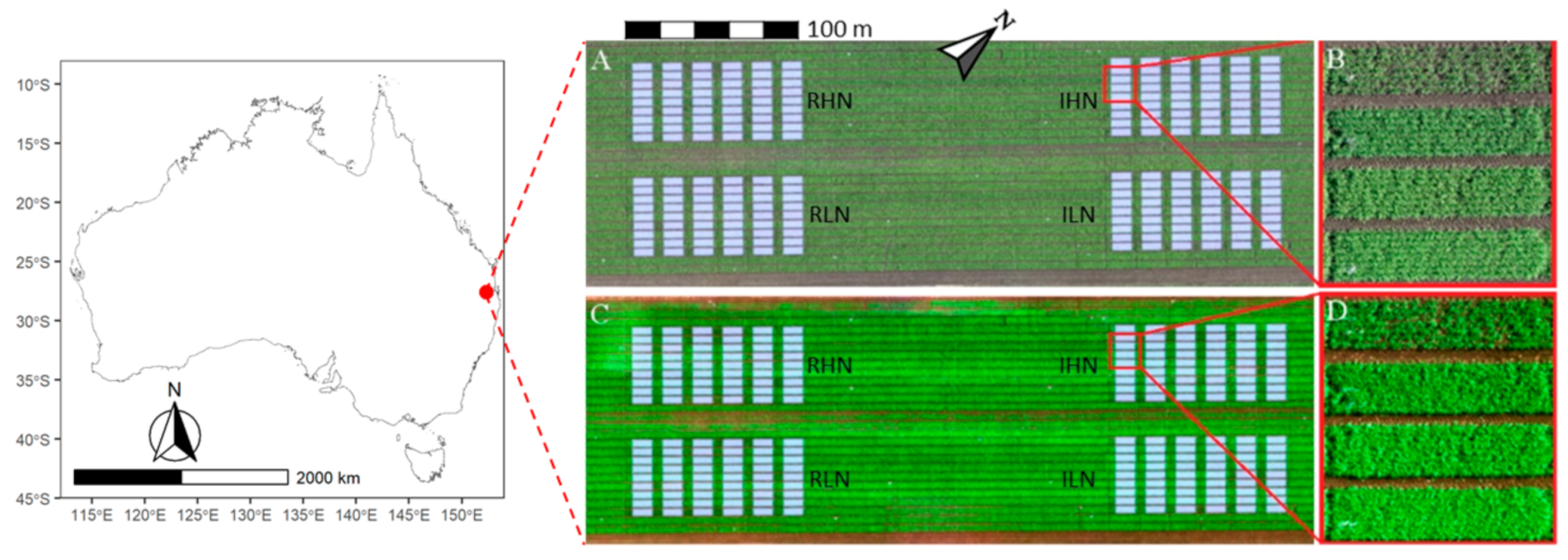
2.1. Field Experiment Setup and Measurements

Field experiments were conducted in 2016 at the CSIRO experimental station located on the Gatton Campus of The University of Queensland (27.57° S, 152.33° E). The experiment comprised 32 treatments, with each treatment having three replicates (i.e., 96 plots in total). Contrasting canopy structures of wheat were established through four factors, including two irrigation treatments (irrigation and rainfed), two nitrogen treatments (high and low nitrogen), two plant densities (150 and 75 plants m−2), and seven cultivars (Gregory, Suntop, 7770, 7770tin, Spitfire, Hartog, and Drysdale). On 21 May 2016, all cultivars were sown at 150 plants m−2, except for 7770tin, which was sown at two plant densities (i.e., 75 and 150 plants m−2). The field was 54 m wide and 161 m long, and divided into four management blocks (Figure 1), which received irrigation and nitrogen treatments. Irrigation was applied 12 times with 310 mm in total for the irrigation treatment, and twice with 60 mm in total for the rainfed treatment. The crop received 220 mm of rainfall between sowing and harvest. Fertilizer was applied at sowing with 205 kg ha−1 for the high-nitrogen and 50 kg ha−1 for the low-nitrogen treatments (Urea, 46% N); this was performed after measuring the pre-planting soil nitrogen, which was at ca. 32.3 kg ha−1 (0 to 0.6 m). Each plot was 2 m wide and 14 m long, and contained seven rows with a row spacing of 22 cm (Figure 1).
Each plot was separated into two subplots; one was used for destructive harvest and the other one for monitoring canopy development by UAV. The harvesting plots were used to measure AGDW and LAI at approximately two-week intervals through the destructive harvesting of an area 1.0 m (4 rows) wide × 0.5 m long (0.50 m wide × 0.5 m long in the first harvest as smaller plants). The leaf area of a subsample of the harvested plants was measured using a leaf area meter (Li-Cor LI-3000, LI-COR Inc., Lincoln, NE, USA). All harvested samples (including leaves) were dried in an oven at 70 °C until the stabilization of their mass and weighed by a scale for dry weight.

2.2. UAV Campaigns and Image Processing

A UAV-based phenotyping platform was used to capture images in the field following protocols developed by [9]. A UAV (Iris+ quadcopter, 3DR Robotic Systems, Palo Alta, CA, USA) mounted with a digital camera (DSC-RX100M3, 5472 × 3648, Sony, Inc., Tokyo, Japan) and a five-band multi-spectral camera (Micasense RedEdge, 1280 × 800, Seattle, WA, USA; https://micasense.com/rededge-mx/; Access date: 17 July 2021) were flown over the wheat field to capture visible and multi-spectral images, respectively. The multi-spectral camera simultaneously captured five images for five bands (i.e., 475 nm for Blue with a 20 nm bandwidth calculated as a full-width half-maximum bandwidth, 560 nm for Green with a 20 nm bandwidth, 668 nm for Red with a 10 nm bandwidth, 840 nm for Near Infrared (NIR) with a 40 nm bandwidth, and 717 nm for Red Edge with a 10 nm bandwidth).
The UAV campaigns were conducted with a controlled flight pattern as substantial image overlap was required to obtain satisfactory ortho-mosaics. Autonomous flight plans (‘lawnmower’ designs) were constructed using a mission planner to have substantial overlap (i.e., 70% forward and 80% side). Ground control points (GCPs) were established across the whole field from the beginning of the growing season (15 GCPs in total). Coordinates of GCPs were recorded before the first flight using the Trimble Geo 7X GPS (http://www.trimble.com; Access date: 17 July 2021). Flight heights were set at 20 or 30 m above ground level (higher at later growth stages) with a flight speed of 3 m per second, resulting in a ground sampling distance of 4 mm (at 20 m flight height) for digital flights, and 13 mm and 18 mm for multi-spectral flights with 20 m and 30 m flight heights, respectively. The total flight time was approximately 10 min. The camera was triggered at a one-second interval, with a shutter speed of <1/1200 s. The ISO was adjusted according to the weather and light conditions (in general, 100 for sunny and 200 for cloudy), and the aperture mode was set to automatic. Extra images were captured for a calibrated reflectance panel at 1 m height immediately before and after each flight in order to calibrate the reflectance data of multi-spectral flights. Both visible and multi-spectral flights were conducted on the same dates (i.e., 9 June, 30 June, 11 July, 19 July, and 1 August 2016; five times in total) before flowering.
The visible and multi-spectral image sets were processed with a cloud-based platform, which is based on Pix4DMapper (Pix4D, SA, Prilly, Switzerland; https://www.pix4d.com/; Access date: 17 July 2021) and designed for UAV survey in agricultural experiments (PhenoCopter; [9]). The image sets were processed to generate undistorted images and ortho-mosaics (e.g., Figure 1) using the same GCP set; multi-spectral ortho-mosaics were calibrated by images of a reflectance panel. A workflow was applied to segment ortho-mosaics of the field into individual plots according to experimental design [27]. Segmented plots were trimmed by a percentage along the four edges (10% for the east, north, and south sides; 25% for the west side) to exclude soil and marginal effects (e.g., Figure 1).

2.3. Calculation of Vegetation Indexes

Vegetation indexes (VIs) and/or ground coverage (GC) were widely used to estimate AGDW and LAI in the literature (e.g., [28]). In this study, seven VIs derived from visible ortho-mosaics (visible index) and six VIs extracted from multi-spectral ortho-mosaics (spectral index) were selected, which were commonly used in previous studies (e.g., [1,5,17,29]). See Table 1 for detailed information on all the VIs, including names, abbreviations, and equations. The spectral index was derived from segmented multi-spectral ortho-mosaics, while the visible index was calculated with normalized digital numbers (Equation (1)) [14,19]:
r = R R + G + B ; g = G R + G + B ; b = B R + G + B  
GC was computed using a decision tree-based machine learning model, which was applied to classify image pixels into two classes, i.e., vegetation and background [30], before computing the GC (Table 1). The model was trained separately for each flight date following three steps. The first step was to create a training set by selecting vegetation and background pixels from undistorted images, with an assigned value of 1 for vegetation and 0 for background. Using the color values (R, G, and B) of pixels in the training set, 18 color features in 6 color spaces were derived, and redundant features were eliminated by a feature selection technique [30]. The decision tree was generated using the selected color features of the training set and the CART classifier. The trained model was then used for image segmentation on undistorted images and the classified images were saved as binary images, with 1 used for vegetive pixels and 0 for background pixels. Finally, a reverse calculation workflow was used to extract the plot areas from classified undistorted images using the information of the corresponding segmented plot on the ortho-mosaic [27]. The final GC of a plot was the average of GCs of extracted plot areas on undistorted images. More information on training a decision tree-based machine learning model for the calculation of GC from UAV imagery was further described in [27]. GC was also treated as a visible index (eight visible indexes in total) as it was extracted from visible ortho-mosaics.

2.4. Model Establishment and Statistical Analysis

The plot-wise VI was summarized as the median value of the pixel-wise VI within each plot. The coefficient of variation of the VIs within each plot was demonstrated in Figure S1, which was normally less than 50% across different VIs and sampling dates. Linear spline interpolations were applied to fit the AGDW and LAI into the dates of UAV flights if the dates of destructive sampling were not matched. The largest difference in the timing of UAV campaigns and destructive measurements was five days; however, this was usually less than three days.
In this study, different modelling strategies were used to build statistical models (i.e., partial least squares regression models) for estimating the AGDW and LAI of each prediction date (i.e., flight date). Modelling strategies were the combinations of sources (Table 1) and temporal combinations of datasets of VIs (Table 2). There were three sources of VIs and three types of temporal combinations of VI datasets so that a total of nine models were built for estimates of each prediction date. The three sources of VIs included visible VIs (eight) derived from visible ortho-mosaics, spectral VIs (six) derived from multi-spectral ortho-mosaics (Table 1), and the collection of all the visible and spectral VIs (i.e., 14 combined VIs).
The three types of temporal combinations of VI datasets were composed of mono-, multi-, and full-temporal datasets of VIs (Type 1, 2, and 3, respectively) and listed in Table 2. Models built with mono-temporal VIs (Type 1) were trained for each prediction date using the VIs derived from UAV imagery of the date. For a particular prediction date, the Type 2 model was built using all the within-season, historical, and multi-temporal datasets of VIs before the prediction date; this means that more historical and multi-temporal datasets were used to build a Type 2 model for a later prediction date. For instance, a Type 2 model for estimations at 40 DAS was built with the historical dataset of 19 DAS, while the Type 2 model for 51 DAS was built using datasets of 19 and 40 DAS. Note that since the earliest prediction day (i.e., 19 DAS) lacked within-season historical VIs, the Type 2 model could not be built for that date (Table 2). The Type 3 model was built with all the available datasets of the season (i.e., five temporal VI datasets) so that this global model was used for estimates of all prediction dates (Table 2).
The partial least squares regression (PLSR) has been applied to estimate phenotypic traits with VIs in multiple studies (e.g., [42]). As a regularized version of the ordinary least squares regressor, PLSR is capable of dealing with high dimensional explanatory variables with a high degree of collinearity through the construction of noncorrelated latent components (factors) from the explanatory variables (VIs), which are relevant to the response variable (AGDW or LAI in this study) and reduce the dimensionality of the variables to avoid overfitting and multi-collinearity issues [43]. More information on the PLSR is further described in [44].
For the model development of each modelling strategy, the dataset was partitioned into two subsets with 75% for model calibration (training set) and the remaining 25% for model validation (testing set). The hyperparameter of the PLSR model (number of components, Ncomp) was tuned using the training set with the repeated grid-search cross-validation method (10 repeats of 8-fold cross-validation in this study). The range of Ncomp depended on the sources of VIs, with Ncomp varying from 1 to 8 for the visible index, 1 to 6 for the spectral index, and 14 for the combined index. The mean cross-validated root mean square error (RMSE; Equation (2)) was then calculated for each Ncomp from the 10 repeats of 8-fold cross-validation of the PLSR. The Ncomp with the smallest mean RMSE was selected as the optimum Ncomp to build the final PLSR model. Finally, the trained model was used to predict the testing set for validation.
Statistical criteria were used to evaluate model performance, including RMSE (Equation (2)) and relative root mean square error (RRMSE; Equation (3)). A lower RMSE or RRMSE often indicates better estimation performance.
RMSE = 1 n i = 1 i = n m i p i 2
RRMSE = RMSE m ¯ × 100 %
where m i and p i are the values of manual measurements and estimates, respectively, n is the number of measurements, and m ¯ is the mean value of manual measurements. To evaluate the effects of the three sources on model performance, the difference between the estimates of any two models built with the three sources at a prediction date was evaluated by the paired t-test at a significance level of 0.05 (i.e., α = 0.05), the null hypothesis being that there was no significant difference between the two groups of estimates. Calculations of VIs, model establishments, and statistical analyses were implemented in R scripts, with the caret [45] and pls [46] package for the training of the PLSR models.

3. Results

3.1. Broad Ranges of AGDW, LAI, and VIs

At each flight date, AGDW and LAI showed obvious variations among the 96 plots (Figure 2, Figures S2 and S3). AGDW rapidly increased from 14.5 ± 3.3 g m−2 (median ± standard deviation) at 19 days after sowing (DAS) to 364.3 ± 67.3 g m−2 at 72 DAS. The values of LAI also rapidly increased until 51 DAS (2.0 ± 0.6 m2 m−2) and then stabilized on average until flowering (2.5 ± 1.0 m2 m−2). AGDW and LAI demonstrated obvious spatial and temporal variations among irrigation and nitrogen treatments at each flight date (Figures S2 and S3).
VIs showed obvious variations among treatments at each flight date. For the visible VIs, ExG, GLI, NGDRI, RGBVI, VARI, and VEG followed a similar dynamic pattern, i.e., values of VIs increased until 51 DAS (0.09 ± 0.02 for ExG, 0.40 ± 0.05 for GLI, 0.38 ± 0.05 for NGDRI, 0.69 ± 0.06 for RGBVI, 0.52 ± 0.06 for VARI, and 2.33 ± 0.25 for VEG) and then decreased until flowering (Figure 3). On the contrary, ExR decreased until 51 DAS (−0.03 ± 0.01) and then increased to −0.01 ± 0.004. GC increased until 59 DAS (0.80 ± 0.10), and then kept almost constant until flowering (0.82 ± 0.10). For spectral indexes, EVI, RDVI and SAVI increased until 51 DAS (0.82 ± 0.18 for EVI, 0.66 ± 0.12 for RDVI and 0.70 ± 0.12 for SAVI) and then decreased until flowering (Figure 4). GNDVI and NDRE increased until 59 DAS (0.79 ± 0.04 for GNDVI and 0.51 ± 0.06 for NDRE) and then slightly changed until flowering (0.80 ± 0.05 for GNDVI and 0.51 ± 0.08 for NDRE). NDVI increased from 0.45 ± 0.04 at 19 DAS to 0.88 ± 0.03 at 51 DAS, and then slightly changed until flowering (0.87 ± 0.04).

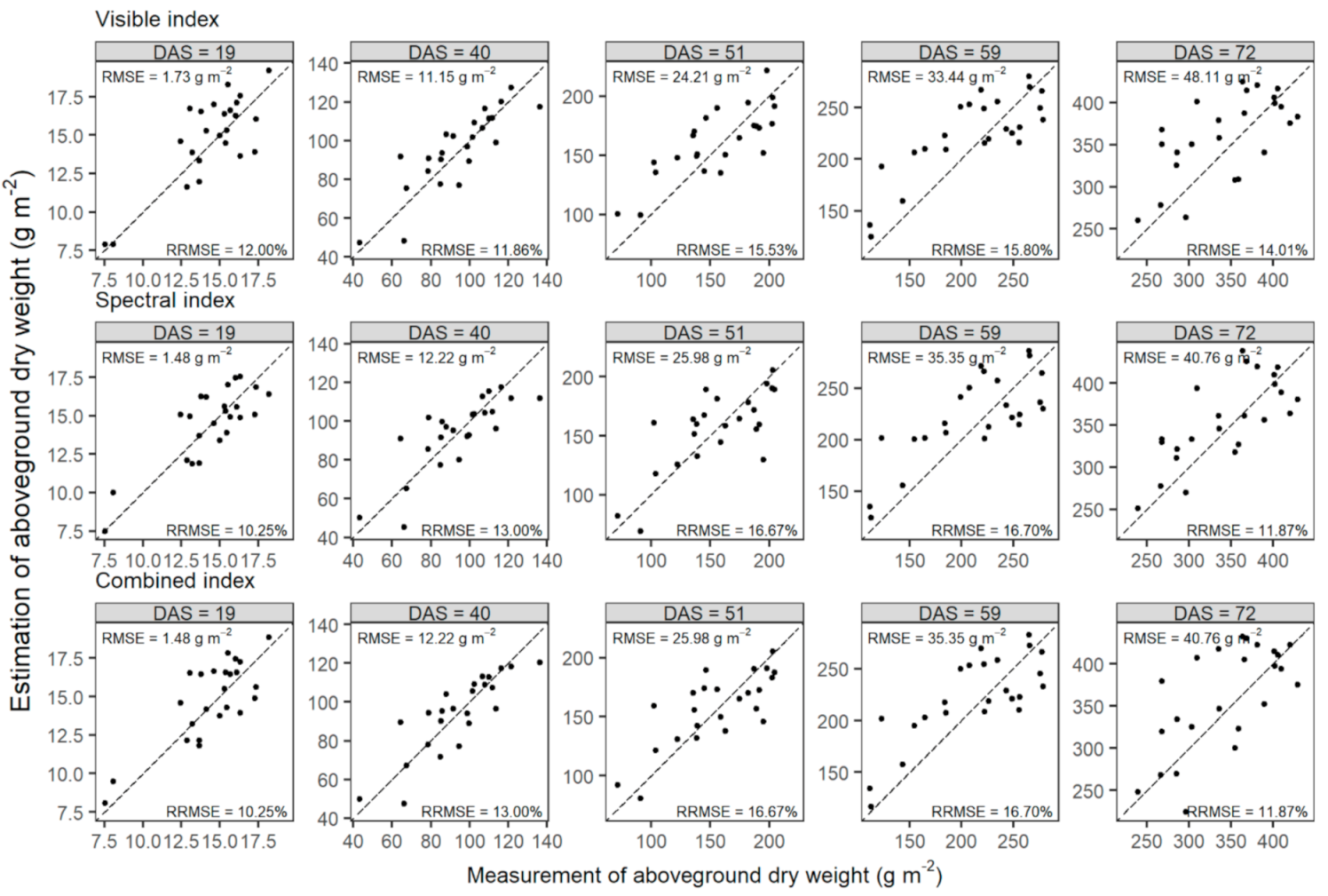
3.2. Estimation of AGDW Using the Mono-Temporal Dataset of VIs

The PLSR models were trained with the mono-temporal datasets of the three sources of VIs (i.e., visible, spectral, and combined indexes) to estimate the AGDW of each prediction date. Figure 5 shows the changes of RRMSE, with an increasing number of components when tuning the hyperparameter (i.e., Ncomp) with training sets. The optimal Ncomp used in these PLSR models and its corresponding RRMSE are summarized in Table 3. The calibration results of the models showed that the three sources of VIs obtained similar results, with the differences in RRMSE ranging between 0.4% and 2.3% when using the three sources of VIs to predict AGDW for the same prediction date (Table 3). The loadings indicated the contribution of each VI to the PLSR models, with the contributions of VIs to these models varying across different prediction dates (Figure S5). Generally, GC and EVI were the most influential VIs in models built to estimate AGDW as these VIs achieved higher loadings across different sources and dates.
The PLSR models were validated using the measurement of AGDW at each prediction date. Models built with the three sources of VIs had similar performances at each date (visible: RRMSE = 11.86% to 15.80%; spectral: RRMSE = 10.25% to 16.70%; combined: RRMSE = 10.25% to 16.70%; Figure 6). The visible index models achieved slightly better estimates at 40, 51, and 59 DAS (RRMSE = 11.867% at 40 DAS; RRMSE = 15.53% at 51 DAS; RRMSE = 15.80% at 59 DAS), and both the spectral and combined indexes produced the highest accuracy at 19 (RRMSE = 10.25%) and 72 DAS (RRMSE = 11.87%). However, there were no significant differences between estimates of any two models built with three sources of VIs at each prediction date (t-test at significance level α = 0.05; data not shown).

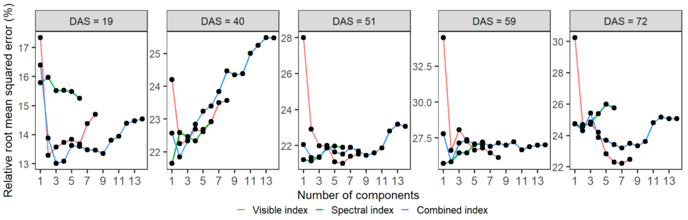
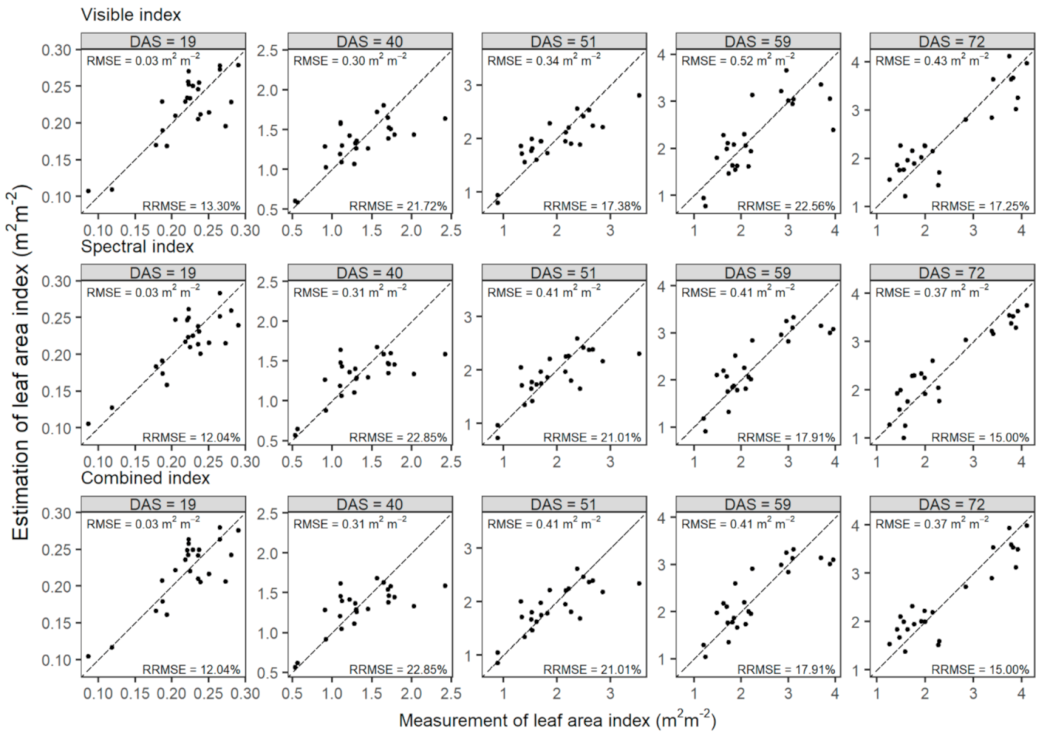
3.3. Estimation of LAI Using the Mono-Temporal Dataset of VIs

The PLSR models were established using mono-temporal datasets of visible, spectral, and combined indexes to estimate LAI at prediction dates. Figure 7 shows the changes of RRMSE with an increasing number of components when tuning the Ncomp with training sets, and the optimal Ncomp with the smallest RRMSE is listed in Table 4. The calibration results of the models indicated that models built with the three sources of VIs obtained similar results, with the differences of RRMSE less than 4.2% when using the three sources of VIs for predicting LAI for the same date (Table 4). The contributions of VIs differed among the PLSR models of different prediction dates. Overall, the most influential VIs on the models were GC and SAVI across different sources and dates (Figure S6).
The PLSR models were tested using the measurement of LAI at each prediction date. The PLSR models built with the three sources of VIs had similar performances at each date (visible: RRMSE = 13.30% to 22.56%; spectral: RRMSE = 12.04% to 22.85%; combined: RRMSE = 13.45% to 22.85%; Figure 8). The visible index obtained slightly better estimates at 40 and 51 DAS (RRMSE = 21.72% at 40 DAS and RRMSE = 17.38% at 51 DAS), while both the spectral and combined indexes outperformed at 19 (RRMSE = 12.04%), 59 (RRMSE = 17.91%), and 72 DAS (RRMSE = 15.00%). However, there were no significant differences among estimates of the three sources of VIs at each prediction date (t-test at significance level α = 0.05; data not shown).

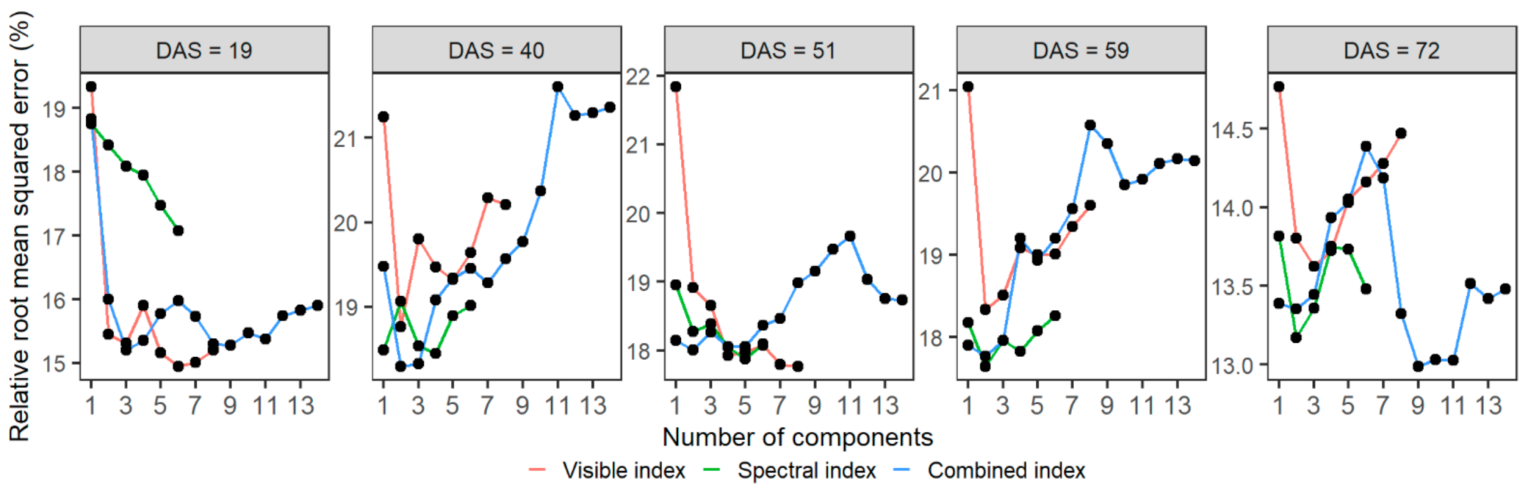
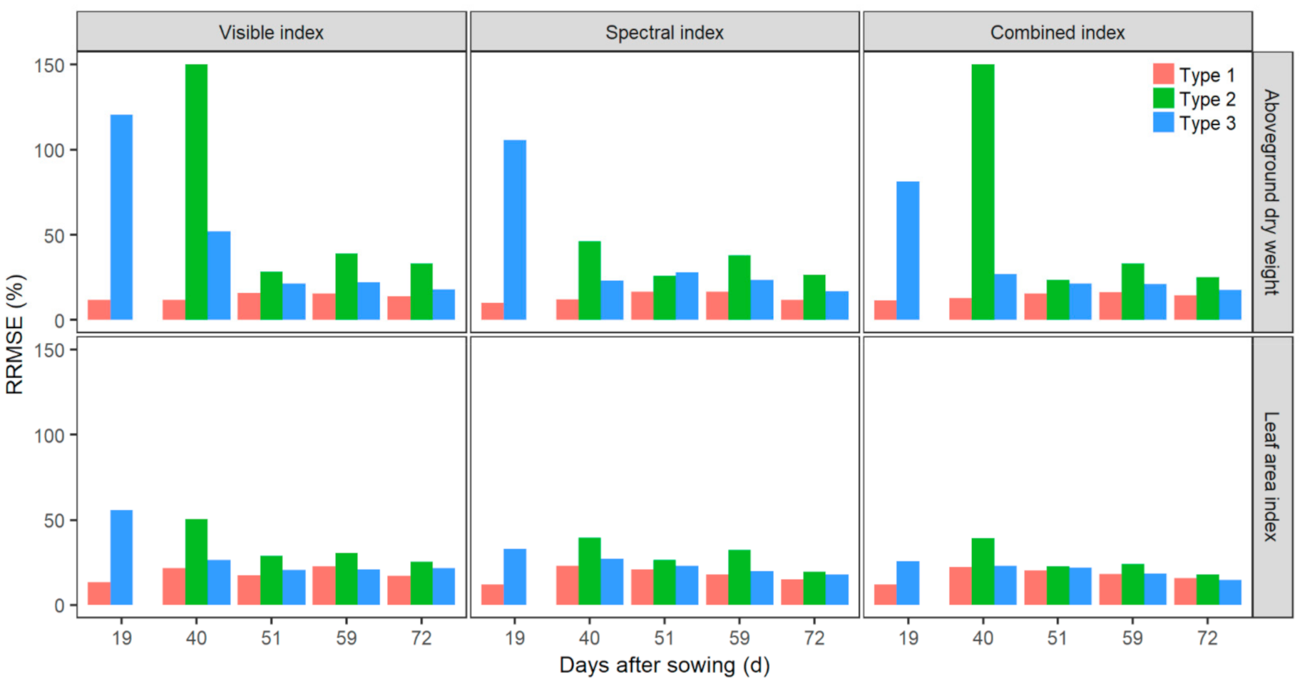
3.4. Evaluation of Temporal Combinations of VI Datasets for Estimates of AGDW and LAI

Models built with different strategies of temporal combinations of VI datasets were used for AGDW and LAI estimates at each prediction date. These modelling strategies were grouped into three types and then evaluated by RRMSE (Figure 9 and Table 2). Type 1 models (using only the prediction date’s VIs, i.e., mono-temporal VIs) generally outperformed the other types of models with the smallest RRMSE; the values of RRMSE ranged from 10.24% to 22.85%. Type 2 models (using within-season multi-temporal datasets of VIs before the prediction date) had the worst performance, with the values of RRMSE normally larger than the corresponding values in Type 1 and Type 3 models. Type 2 models also obtained a large variation of RRMSE, ranging from 17.99% to 150.26%. Type 3 models (using all the temporal datasets of the season) had slightly worse performances (RRMSE from 14.61% to 120.70%) than Type 1 models, except at 19 and 40 DAS as the earliest prediction dates. The differences of RRMSE between the two types of models mainly varied between 0.40% and 14.14%, and 20 out of 30 cases (except cases at 19 and 40 DAS) were less than 10%; some models of Type 3 (2 out of 30 cases) had even smaller RRMSE than the corresponding Type 1 models. Values of RRMSE of Type 3 models generally decreased from 19 DAS to 72 DAS for each source of VIs.

4. Discussion

4.1. AGDW and LAI of Wheat Were Accurately Estimated by Statistical Models Built with UAV-Derived VIs

In this study, the effects of modelling strategies involving the dataset composition of explanatory variables (i.e., sources and temporal combinations of datasets of UAV-derived VIs) on the estimates of AGDW and LAI were evaluated. Three sources of VIs (i.e., visible index, spectral index, and the combination of all the visible and spectral indexes) were applied to estimate AGDW and LAI with PLSR models. These models built with mono-temporal datasets of VIs showed the ability to accurately estimate AGDW (RRMSE as small as 10.25%; Figure 6) and LAI (RRMSE as small as 12.04%; Figure 8) across prediction dates.
The performances of estimation models in this study were comparable to previous studies of AGDW [25,28,42] and LAI [1,47]. It should be noted that the measurements from different treatments (i.e., irrigation, nitrogen, and cultivar treatments) with contrasting canopy structures were pooled together to build models, as this study intended to obtain a broad range of AGDW, LAI, and VIs (Figure 2, Figure 3 and Figure 4, Figures S2 and S3) in order to build more comprehensive and robust models. However, the relationship between the explanatory variable (AGDW or LAI) and the response variables (VIs) might be different among treatments, so that pooling them together might introduce errors and uncertainty in coefficient estimates (different models might be mixed).
The estimation accuracy of AGDW and LAI could be improved by introducing new data sources and data processing techniques. Hyperspectral VIs computed from specific narrow bands have shown great potential in estimating AGDW and LAI as they are more sensitive to vegetation [42,48]. Data fusion techniques utilize both the strength and compensation of individual data sources and thus provide more accurate estimates such as fusing VIs and the three-dimensional (3D) information of vegetation structure provided by LiDAR, Radar, ultrasonic sensors, or 3D reconstruction from image sequences [1,28,48,49]. As alternatives to PLSR, machine learning algorithms such as support vector machine [50] and random forest [25,48] may offer better estimates of plant traits than normal statistical models (e.g., PLSR models). But their applicability may be limited as their results are difficult to interpret given that they do not structure knowledge with mathematical functions in order to express modelling processes and that they require relatively big datasets to train models.

4.2. UAV-Derived Visible VIs Are Alternative to Multispectral VIs for In-Season Estimates of AGDW and LAI

No obvious advantages were observed in this study for the use of multi-spectral indexes instead of visible indexes to build models for estimating AGDW and LAI (Figure 6 and Figure 8). The models built with the three sources of mono-temporal VIs generally obtained similar estimates of AGDW and LAI, and the visible index slightly outperformed the other two sources of VIs at most prediction dates (3 out of 5 dates for both AGDW and LAI). Therefore, these results did not provide support for our hypothesis that the spectral VIs would outperform visible VIs in in-season estimates of AGDW and LAI. This may be due to the fact that visible VIs were derived from high-resolution images (5472 × 3648 in this study) containing canopy structural information and rich texture information, resulting in less effects of mixed pixels on the VI calculations and obtaining relatively clear phenotypes of crops like GC [14,25,51]. Multi-spectral sensors can offer more spectral information indicating physiological characteristics of vegetation, but the saturation effect could impair the estimates of phenotypic traits when using these sensors to screen dense vegetation canopies. Multi-spectral imageries normally have relatively coarse resolutions (1280 × 800 in this study), which might result in more severe mixed pixel problems that cause inaccurate extractions of VIs. Unlike the visible indexes calculated from uncalibrated visible ortho-mosaics, multi-spectral ortho-mosaics were rectified by reflectance panels, which could reduce the influence of meteorological conditions on spectral imaging and thus improve the accuracy of VIs.
It is convenient to choose the most suitable sensor based on the requirement of a study. Our results suggested that visible imagery could be an alternative to multi-spectral imagery for the phenotyping of AGDW and LAI with UAV surveys, and also for phenotyping other traits in previous literature (e.g., [52]). Some studies suggested that combinations of multiple variables may improve the estimation accuracy of vegetation parameters [48,53]. The combined index in this study obtained similar estimates to the other two sources of VIs and did not substantially improve the estimation performance (Figure 6, Figure 8, and Figure 9). This might be due to the high correlations among these indexes (Figure S4) and the dimension reduction nature of PLSR (Table 3 and Table 4) [43,44].
The VIs showed different contributions to the PLSR models for estimating AGDW and LAI at different dates (Figures S5 and S6). Overall, GC was the most influential index. GC could serve as an overall estimator for AGDW and LAI, which was consistent with previous studies that showed that GC is correlated with AGDW and LAI before flowering (e.g., [28]). The varying contributions of VIs might be due to the fact that most VIs tended to be species-specific with different canopy architectures and leaf structures [17] and may be limited to certain growth stages [18,29].

4.3. Introducing More Temporal VI Datasets Inconsistently Affected Model Performances of Phenotypic Estimates

The model performance was also impacted by the temporal combinations of VIs for estimates of AGDW and LAI (Figure 9). Previous studies have shown that multi-temporal VIs could improve the prediction accuracy of phenotypic traits as the use of multi-temporal remotely sensed data could mitigate the effects of soil background and can provide more useful information [19,21,21,54]. Our results showed that Type 2 models (built with within-season historical multi-temporal datasets of VIs before prediction dates) had the worst performances with large variations of RRMSE values (Figure 9). This might be due to the fact that prior knowledge or skill could not be extended to the current prediction date as the dynamic plant growth, leading to the change of relationships between phenotypic traits and reflectance of canopy structure [17], especially for the early growth stages. Type 3 models (built with all the within-season temporal datasets of VIs) obtained similar estimates to (or potentially better than) Type 1 models (built with mono-temporal VIs of the prediction date). However, Type 3 did not always substantially improve the performance, especially when it was used for early season estimates (e.g., 19 DAS) (Figure 9).
These results provide support for our second hypothesis that models built with mono-temporal datasets of VIs will be superior to models using multi- and full-temporal datasets in estimates of AGDW and LAI. Integrations of temporal datasets might include noise values introduced by the contrasting reflectance of the canopy structure as plant growth, VI calculation biased by effects of mixed pixels and saturation, and the representativeness of sample plots. In contrast, Type 1 models could minimize these impacts as the highest correlations between plots for building models and plots for estimates in a trial and between current biophysical variables (i.e., AGDW or LAI) and current reflectance of canopies. From a practical perspective, Type 1 models were preferred when the UAV imagery for the prediction date was available for in-season estimates of phenotypic traits [21]. However, Type 1 models require recalibrations at new prediction dates, so global models (Type 3) are alternatives and more practical as they allow for the avoidance of frequent model calibrations [25,26]; however, they might not be preferable for early growth stages (e.g., 19 DAS; Figure 9) as the model establishments could be biased by larger values of phenotypic traits collected at later stages (Figure 2). Moreover, global models were not feasible for in-season estimates as they were established after the season.

4.4. Self-Calibration Modelling Strategy Was Useful for in-Season Phenotyping of Crop Traits with UAV Surveys

Modern breeding programs require phenotyping thousands of plots in multi-environment trials distributed across target regions [7,55,56]. It is a challenge to cost- and time-efficiently evaluate phenotypic traits under field conditions by traditional phenotyping methods, which are expensive, laborious, and time-consuming. UAV-based platforms are flexible in the temporal and spatial resolution of data collection and can easily visit multiple locations, which can greatly broaden their applicability in high-throughput phenotyping [7,9,57]. This study demonstrated that both the UAV-derived visible and multi-spectral VIs were reliable for the high-throughput phenotyping of AGDW and LAI of wheat trials (Figure 6, Figure 8 and Figure 9).
Statistical models are normally required for the estimation or prediction of phenotypic traits using UAV-based platforms in breeding programs, which are developed with manually measured data from destructive sampling (response variables; e.g., AGDW and LAI) and quantitative values of diverse properties (explanatory variables; e.g., VIs) extracted from UAV imagery. However, destructive sampling may be prohibitive in costs or small breeding plots may not allow enough for multi-temporal destructive sampling in a breeding program [58]. Moreover, models should be built with datasets from only one UAV campaign for within-season estimates in breeding and precision agriculture [29]. This study demonstrated the potential of models built with mono-temporal datasets of VIs (Type 1 models) for timely monitoring and accurate real-time estimates, as they generally outperformed other types of models built with multi- and full-temporal datasets of VIs (Type 2 and Type 3 models) for AGDW and LAI estimates (Figure 9 and Table 2). To address issues of destructive sampling for the establishment of statistical models, this study recommends a self-calibration strategy to build statistical models, i.e., each plot should be separated into two subplots, in which one is used for destructive sampling and the other for extracting quantitative values of diverse properties [59]. When applying UAV-based high-throughput phenotyping in breeding programs, this strategy can be adjusted to build statistical models by adding check lines with larger plots for multi-temporal destructive sampling and UAV monitoring; the established statistical models can then be used to estimate phenotypic traits of other breeding plots. The self-calibration strategy combined with the mono-temporal dataset can offer a pragmatic, robust, and universal approach to high-throughput phenotyping of crop traits with UAV surveys.

5. Conclusions

UAV-based remote sensing provides cost-effective and non-destructive methods for the high-throughput phenotyping of crop traits through the integration of UAV-derived VIs with statistical models. This study evaluated the effects of the dataset composition of explanatory variables (i.e., sources and temporal combinations of UAV-derived VIs) on estimates of AGDW and LAI. The results demonstrated that the use of UAV-derived visible VIs can be an alternative to multi-spectral VIs for in-season estimates of AGDW and LAI. The multi-temporal datasets of VIs did not substantially improve the accuracy of estimates. The combination of the modelling strategy of using a mono-temporal VI dataset and the self-calibration method demonstrated the potential for in-season estimates of AGDW and LAI in breeding or agronomy trials.
Further research needs to be carried out to improve this study in terms of data availability. As this study was conducted using data collected from a wheat trial, the outcomes might be site- and/or specie-specific. More data from different sites, crops, and growing seasons could be used to confirm the conclusions drawn in this study. Although UAV-based remote sensing was feasible for the accurate assessments of crop traits in this study, the integration of complementary/ancillary data (e.g., growing degree days, temperature, and plant height) with UAV-derived VIs using statistical modelling techniques to obtain more accurate estimates should be investigated.

Supplementary Materials

The following are available online at https://www.mdpi.com/article/10.3390/rs13142827/s1. Figure S1: Spatial distribution of coefficient of variation of vegetation indexes of each plot of the wheat trial at different dates (represented by days after sowing, DAS) before flowering; Figure S2: Spatial distribution of the aboveground dry weight of the wheat trial at different dates (represented by days after sowing, DAS) before flowering; Figure S3: Spatial distribution of the leaf area index of the wheat trial at different dates (represented by days after sowing, DAS) before flowering; Figure S4: Spearman correlations among aboveground dry weight (AGDW), leaf area index (LAI), and vegetation indexes (VIs) of the wheat trial at each prediction date (represented by days after sowing, DAS) before flowering; Figure S5: Loadings of vegetation indexes in PLSR models for estimating aboveground dry weight at different prediction dates (represented by days after sowing, DAS; colored lines) before flowering; Figure S6: Loadings of vegetation indexes in PLSR models for estimating leaf area index at different prediction dates (represented by days after sowing, DAS; colored lines) before flowering.

Author Contributions

P.H.: Conceptualization, methodology, software, investigation, writing—original draft, writing—review and editing. S.C.C.: Conceptualization, funding acquisition, writing—review and editing. H.J.: Writing—review and editing. Y.G.: Writing—review and editing. B.Z.: Conceptualization, supervision, project administration, writing—review and editing. All authors have read and agreed to the published version of the manuscript.

Funding

This research was funded by Grains Research and Development Corporation (grant number CSP00179) and the National Natural Science Foundation of China (grant number 31771678). The APC was funded by Grains Research and Development Corporation.

Data Availability Statement

The data presented in this study are available on request from the corresponding author.

Acknowledgments

This research was supported by CSIRO, with P.H. and Y.G. receiving funding from the National Natural Science Foundation of China (Grant no. 31771678). This field experiment was supported by the Grains Research and Development Corporation (Grant no. CSP00179). We thank Di He (CSIRO) for discussions on statistics and Yang Chen (CSIRO) for suggestions on revising the manuscript.

Conflicts of Interest

The authors declare no conflict of interest.

References

  1. Jin, X.; Yang, G.; Xu, X.; Yang, H.; Feng, H.; Li, Z.; Shen, J.; Zhao, C.; Lan, Y. Combined Multi-Temporal Optical and Radar Parameters for Estimating LAI and Biomass in Winter Wheat Using HJ and RADARSAR-2 Data. Remote Sens. 2015, 7, 3251. [Google Scholar] [CrossRef] [Green Version]
  2. Montes, J.M.; Technow, F.; Dhillon, B.S.; Mauch, F.; Melchinger, A.E. High-Throughput Non-Destructive Biomass Determination during Early Plant Development in Maize under Field Conditions. Field Crops Res. 2011, 121, 268–273. [Google Scholar] [CrossRef]
  3. Araus, J.L.; Cairns, J.E. Field High-Throughput Phenotyping: The New Crop Breeding Frontier. Trends Plant Sci. 2014, 19, 52–61. [Google Scholar] [CrossRef]
  4. ten Harkel, J.; Bartholomeus, H.; Kooistra, L. Biomass and Crop Height Estimation of Different Crops Using UAV-Based Lidar. Remote Sens. 2020, 12, 17. [Google Scholar] [CrossRef] [Green Version]
  5. Yue, J.; Feng, H.; Li, Z.; Zhou, C.; Xu, K. Mapping Winter-Wheat Biomass and Grain Yield Based on a Crop Model and UAV Remote Sensing. Int. J. Remote Sens. 2021, 42, 1577–1601. [Google Scholar] [CrossRef]
  6. Kamenova, I.; Dimitrov, P. Evaluation of Sentinel-2 Vegetation Indices for Prediction of LAI, FAPAR and FCover of Winter Wheat in Bulgaria. Eur. J. Remote Sens. 2021, 54, 89–108. [Google Scholar] [CrossRef]
  7. Sankaran, S.; Khot, L.R.; Espinoza, C.Z.; Jarolmasjed, S.; Sathuvalli, V.R.; Vandemark, G.J.; Miklas, P.N.; Carter, A.H.; Pumphrey, M.O.; Knowles, N.R.; et al. Low-Altitude, High-Resolution Aerial Imaging Systems for Row and Field Crop Phenotyping: A Review. Eur. J. Agron. 2015, 70, 112–123. [Google Scholar] [CrossRef]
  8. Liu, F.; Hu, P.; Zheng, B.; Duan, T.; Zhu, B.; Guo, Y. A Field-Based High-Throughput Method for Acquiring Canopy Architecture Using Unmanned Aerial Vehicle Images. Agric. For. Meteorol. 2021, 296, 108231. [Google Scholar] [CrossRef]
  9. Chapman, S.C.; Merz, T.; Chan, A.; Jackway, P.; Hrabar, S.; Dreccer, M.F.; Holland, E.; Zheng, B.; Ling, T.J.; Jimenez-Berni, J. Pheno-Copter: A Low-Altitude, Autonomous Remote-Sensing Robotic Helicopter for High-Throughput Field-Based Phenotyping. Agronomy 2014, 4, 279. [Google Scholar] [CrossRef] [Green Version]
  10. Hu, P.; Chapman, S.C.; Zheng, B. Coupling of Machine Learning Methods to Improve Estimation of Ground Coverage from Unmanned Aerial Vehicle (UAV) Imagery for High-Throughput Phenotyping of Crops. Funct. Plant Biol. 2021. [Google Scholar] [CrossRef]
  11. Hu, P.; Chapman, S.C.; Wang, X.; Potgieter, A.; Duan, T.; Jordan, D.; Guo, Y.; Zheng, B. Estimation of Plant Height Using a High Throughput Phenotyping Platform Based on Unmanned Aerial Vehicle and Self-Calibration: Example for Sorghum Breeding. Eur. J. Agron. 2018, 95, 24–32. [Google Scholar] [CrossRef]
  12. Lyu, B.; Smith, S.D.; Xue, Y.; Rainey, K.M.; Cherkauer, K. An Efficient Pipeline for Crop Image Extraction and Vegetation Index Derivation Using Unmanned Aerial Systems. Trans. ASABE 2020, 63, 1133–1146. [Google Scholar] [CrossRef]
  13. Hunt, E.R.; Daughtry, C.S.T.; Eitel, J.U.; Long, D.S. Remote Sensing Leaf Chlorophyll Content Using a Visible Band Index. Agron. J. 2011, 103, 1090–1099. [Google Scholar] [CrossRef] [Green Version]
  14. Torres-Sánchez, J.; Peña, J.M.; de Castro, A.I.; López-Granados, F. Multi-Temporal Mapping of the Vegetation Fraction in Early-Season Wheat Fields Using Images from UAV. Comput. Electron. Agric. 2014, 103, 104–113. [Google Scholar] [CrossRef]
  15. Madasa, A.; Orimoloye, I.R.; Ololade, O.O. Application of Geospatial Indices for Mapping Land Cover/Use Change Detection in a Mining Area. J. Afr. Earth Sci. 2021, 175, 104108. [Google Scholar] [CrossRef]
  16. Huete, A.; Didan, K.; Miura, T.; Rodriguez, E.P.; Gao, X.; Ferreira, L.G. Overview of the Radiometric and Biophysical Performance of the MODIS Vegetation Indices. Remote Sens. Environ. 2002, 83, 195–213. [Google Scholar] [CrossRef]
  17. Viña, A.; Gitelson, A.A.; Nguy-Robertson, A.L.; Peng, Y. Comparison of Different Vegetation Indices for the Remote Assessment of Green Leaf Area Index of Crops. Remote Sens. Environ. 2011, 115, 3468–3478. [Google Scholar] [CrossRef]
  18. Bendig, J.; Yu, K.; Aasen, H.; Bolten, A.; Bennertz, S.; Broscheit, J.; Gnyp, M.L.; Bareth, G. Combining UAV-Based Plant Height from Crop Surface Models, Visible, and near Infrared Vegetation Indices for Biomass Monitoring in Barley. Int. J. Appl. Earth Obs. Geoinf. 2015, 39, 79–87. [Google Scholar] [CrossRef]
  19. Zhou, X.; Zheng, H.B.; Xu, X.Q.; He, J.Y.; Ge, X.K.; Yao, X.; Cheng, T.; Zhu, Y.; Cao, W.X.; Tian, Y.C. Predicting Grain Yield in Rice Using Multi-Temporal Vegetation Indices from UAV-Based Multispectral and Digital Imagery. ISPRS J. Photogramm. Remote Sens. 2017, 130, 246–255. [Google Scholar] [CrossRef]
  20. Gracia-Romero, A.; Kefauver, S.C.; Vergara-Díaz, O.; Zaman-Allah, M.A.; Prasanna, B.M.; Cairns, J.E.; Araus, J.L. Comparative Performance of Ground vs. Aerially Assessed RGB and Multispectral Indices for Early-Growth Evaluation of Maize Performance under Phosphorus Fertilization. Front. Plant Sci. 2017, 8. [Google Scholar] [CrossRef] [Green Version]
  21. Wang, L.; Tian, Y.; Yao, X.; Zhu, Y.; Cao, W. Predicting Grain Yield and Protein Content in Wheat by Fusing Multi-Sensor and Multi-Temporal Remote-Sensing Images. Field Crops Res. 2014, 164, 178–188. [Google Scholar] [CrossRef]
  22. Johnson, D.M. An Assessment of Pre- and within-Season Remotely Sensed Variables for Forecasting Corn and Soybean Yields in the United States. Remote Sens. Environ. 2014, 141, 116–128. [Google Scholar] [CrossRef]
  23. Gnyp, M.L.; Miao, Y.; Yuan, F.; Ustin, S.L.; Yu, K.; Yao, Y.; Huang, S.; Bareth, G. Hyperspectral Canopy Sensing of Paddy Rice Aboveground Biomass at Different Growth Stages. Field Crops Res. 2014, 155, 42–55. [Google Scholar] [CrossRef]
  24. Ghosal, S.; Zheng, B.; Chapman, S.C.; Potgieter, A.B.; Jordan, D.R.; Wang, X.; Singh, A.K.; Singh, A.; Hirafuji, M.; Ninomiya, S.; et al. A Weakly Supervised Deep Learning Framework for Sorghum Head Detection and Counting. Plant Phenomics 2019, 2019, 1525874. [Google Scholar] [CrossRef] [Green Version]
  25. Cen, H.; Wan, L.; Zhu, J.; Li, Y.; Li, X.; Zhu, Y.; Weng, H.; Wu, W.; Yin, W.; Xu, C.; et al. Dynamic Monitoring of Biomass of Rice under Different Nitrogen Treatments Using a Lightweight UAV with Dual Image-Frame Snapshot Cameras. Plant Methods 2019, 15, 32. [Google Scholar] [CrossRef] [PubMed]
  26. Lu, N.; Zhou, J.; Han, Z.; Li, D.; Cao, Q.; Yao, X.; Tian, Y.; Zhu, Y.; Cao, W.; Cheng, T. Improved Estimation of Aboveground Biomass in Wheat from RGB Imagery and Point Cloud Data Acquired with a Low-Cost Unmanned Aerial Vehicle System. Plant Methods 2019, 15, 17. [Google Scholar] [CrossRef] [Green Version]
  27. Duan, T.; Zheng, B.; Guo, W.; Ninomiya, S.; Guo, Y.; Chapman, S.C. Comparison of Ground Cover Estimates from Experiment Plots in Cotton, Sorghum and Sugarcane Based on Images and Ortho-Mosaics Captured by UAV. Funct. Plant Biol. 2017, 44, 169–183. [Google Scholar] [CrossRef]
  28. Schirrmann, M.; Hamdorf, A.; Garz, A.; Ustyuzhanin, A.; Dammer, K.H. Estimating Wheat Biomass by Combining Image Clustering with Crop Height. Comput. Electron. Agric. 2016, 121, 374–384. [Google Scholar] [CrossRef]
  29. Tilly, N.; Aasen, H.; Bareth, G. Fusion of Plant Height and Vegetation Indices for the Estimation of Barley Biomass. Remote Sens. 2015, 7, 1449. [Google Scholar] [CrossRef] [Green Version]
  30. Guo, W.; Rage, U.K.; Ninomiya, S. Illumination Invariant Segmentation of Vegetation for Time Series Wheat Images Based on Decision Tree Model. Comput. Electron. Agric. 2013, 96, 58–66. [Google Scholar] [CrossRef]
  31. Louhaichi, M.; Borman, M.M.; Johnson, D.E. Spatially Located Platform and Aerial Photography for Documentation of Grazing Impacts on Wheat. Geocarto Int. 2001, 16, 65–70. [Google Scholar] [CrossRef]
  32. Tucker, C.J. Red and Photographic Infrared Linear Combinations for Monitoring Vegetation. Remote Sens. Environ. 1979, 8, 127–150. [Google Scholar] [CrossRef] [Green Version]
  33. Gitelson, A.A.; Kaufman, Y.J.; Stark, R.; Rundquist, D. Novel Algorithms for Remote Estimation of Vegetation Fraction. Remote Sens. Environ. 2002, 80, 76–87. [Google Scholar] [CrossRef] [Green Version]
  34. Hague, T.; Tillett, N.D.; Wheeler, H. Automated Crop and Weed Monitoring in Widely Spaced Cereals. Precis. Agric. 2006, 7, 21–32. [Google Scholar] [CrossRef]
  35. Woebbecke, D.M.; Meyer, G.E.; Von Bargen, K.; Mortensen, D.A. Color Indices for Weed Identification under Various Soil, Residue, and Lighting Conditions. Trans. ASAE USA 1995, 38, 259–269. [Google Scholar] [CrossRef]
  36. Meyer, G.E.; Neto, J.C. Verification of Color Vegetation Indices for Automated Crop Imaging Applications. Comput. Electron. Agric. 2008, 63, 282–293. [Google Scholar] [CrossRef]
  37. Rouse, J.W.; Hass, R.H.; Schell, J.A.; Deering, D.W. Monitoring Vegetation Systems in the Great Plains with ERTS. In Proceedings of the Third ERTS Symposium, NASA special publication, Washington, DC, USA, 10–14 December 1973; Volume 1, pp. 309–317. [Google Scholar]
  38. Gitelson, A.A.; Kaufman, Y.J.; Merzlyak, M.N. Use of a Green Channel in Remote Sensing of Global Vegetation from EOS-MODIS. Remote Sens. Environ. 1996, 58, 289–298. [Google Scholar] [CrossRef]
  39. Huete, A.R. A Soil-Adjusted Vegetation Index (SAVI). Remote Sens. Environ. 1988, 25, 295–309. [Google Scholar] [CrossRef]
  40. Gitelson, A.; Merzlyak, M.N. Quantitative Estimation of Chlorophyll-a Using Reflectance Spectra: Experiments with Autumn Chestnut and Maple Leaves. J. Photochem. Photobiol. B Biol. 1994, 22, 247–252. [Google Scholar] [CrossRef]
  41. Roujean, J.L.; Breon, F.M. Estimating PAR Absorbed by Vegetation from Bidirectional Reflectance Measurements. Remote Sens. Environ. 1995, 51, 375–384. [Google Scholar] [CrossRef]
  42. Fu, Y.; Yang, G.; Wang, J.; Song, X.; Feng, H. Winter Wheat Biomass Estimation Based on Spectral Indices, Band Depth Analysis and Partial Least Squares Regression Using Hyperspectral Measurements. Comput. Electron. Agric. 2014, 100, 51–59. [Google Scholar] [CrossRef]
  43. Clevers, J.G.P.W.; Van der Heijden, G.W.A.M.; Verzakov, S.; Schaepman, M.E. Estimating Grassland Biomass Using SVM Band Shaving of Hyperspectral Data. Photogramm. Eng. Remote Sens. 2007, 73, 1141–1148. [Google Scholar] [CrossRef] [Green Version]
  44. Geladi, P.; Kowalski, B.R. Partial Least-Squares Regression: A Tutorial. Anal. Chim. Acta 1986, 185, 1–17. [Google Scholar] [CrossRef]
  45. Kuhn, M. Building Predictive Models in R Using the Caret Package. J. Stat. Softw. 2008, 28, 1–26. [Google Scholar] [CrossRef] [Green Version]
  46. Mevik, B.; Wehrens, R. The Pls Package: Principal Component and Partial Least Squares Regression in R. J. Stat. Softw. 2007, 18, 1–24. [Google Scholar] [CrossRef] [Green Version]
  47. Nguy-Robertson, A.L.; Peng, Y.; Gitelson, A.A.; Arkebauer, T.J.; Pimstein, A.; Herrmann, I.; Karnieli, A.; Rundquist, D.C.; Bonfil, D.J. Estimating Green LAI in Four Crops: Potential of Determining Optimal Spectral Bands for a Universal Algorithm. Agric. For. Meteorol. 2014, 192–193, 140–148. [Google Scholar] [CrossRef]
  48. Li, W.; Niu, Z.; Chen, H.; Li, D.; Wu, M.; Zhao, W. Remote Estimation of Canopy Height and Aboveground Biomass of Maize Using High-Resolution Stereo Images from a Low-Cost Unmanned Aerial Vehicle System. Ecol. Indic. 2016, 67, 637–648. [Google Scholar] [CrossRef]
  49. Moeckel, T.; Safari, H.; Reddersen, B.; Fricke, T.; Wachendorf, M. Fusion of Ultrasonic and Spectral Sensor Data for Improving the Estimation of Biomass in Grasslands with Heterogeneous Sward Structure. Remote Sens. 2017, 9, 98. [Google Scholar] [CrossRef] [Green Version]
  50. Marabel, M.; Alvarez-Taboada, F. Spectroscopic Determination of Aboveground Biomass in Grasslands Using Spectral Transformations, Support Vector Machine and Partial Least Squares Regression. Sensors 2013, 13, 27. [Google Scholar] [CrossRef] [Green Version]
  51. Hu, P.; Guo, W.; Chapman, S.C.; Guo, Y.; Zheng, B. Pixel Size of Aerial Imagery Constrains the Applications of Unmanned Aerial Vehicle in Crop Breeding. ISPRS J. Photogramm. Remote Sens. 2019, 154, 1–9. [Google Scholar] [CrossRef]
  52. Santini, F.; Kefauver, S.C.; de Dios, V.R.; Araus, J.L.; Voltas, J. Using Unmanned Aerial Vehicle-Based Multispectral, RGB and Thermal Imagery for Phenotyping of Forest Genetic Trials: A Case Study in Pinus Halepensis. Ann. Appl. Biol. 2019, 174, 262–276. [Google Scholar] [CrossRef] [Green Version]
  53. Aasen, H.; Burkart, A.; Bolten, A.; Bareth, G. Generating 3D Hyperspectral Information with Lightweight UAV Snapshot Cameras for Vegetation Monitoring: From Camera Calibration to Quality Assurance. ISPRS J. Photogramm. Remote Sens. 2015, 108, 245–259. [Google Scholar] [CrossRef]
  54. Li, F.; Jiang, L.; Wang, X.; Zhang, X.; Zheng, J.; Zhao, Q. Estimating Grassland Aboveground Biomass Using Multitemporal MODIS Data in the West Songnen Plain, China. J. Appl. Remote Sens. 2013, 7, 073546. [Google Scholar] [CrossRef]
  55. Cobb, J.N.; DeClerck, G.; Greenberg, A.; Clark, R.; McCouch, S. Next-Generation Phenotyping: Requirements and Strategies for Enhancing Our Understanding of Genotype–Phenotype Relationships and Its Relevance to Crop Improvement. Theor. Appl. Genet. 2013, 126, 867–887. [Google Scholar] [CrossRef] [PubMed] [Green Version]
  56. Guo, W.; Carroll, M.E.; Singh, A.; Swetnam, T.L.; Merchant, N.; Sarkar, S.; Singh, A.K.; Ganapathysubramanian, B. UAS-Based Plant Phenotyping for Research and Breeding Applications. Plant Phenomics 2021, 2021. [Google Scholar] [CrossRef] [PubMed]
  57. Yang, G.; Liu, J.; Zhao, C.; Li, Z.; Huang, Y.; Yu, H.; Xu, B.; Yang, X.; Zhu, D.; Zhang, X.; et al. Unmanned Aerial Vehicle Remote Sensing for Field-Based Crop Phenotyping: Current Status and Perspectives. Front. Plant Sci. 2017, 8. [Google Scholar] [CrossRef]
  58. Greaves, H.E.; Vierling, L.A.; Eitel, J.U.H.; Boelman, N.T.; Magney, T.S.; Prager, C.M.; Griffin, K.L. Estimating Aboveground Biomass and Leaf Area of Low-Stature Arctic Shrubs with Terrestrial LiDAR. Remote Sens. Environ. 2015, 164, 26–35. [Google Scholar] [CrossRef]
  59. Chapman, S.C.; Zheng, B.; Potgieter, A.; Guo, W.; Frederic, B.; Liu, S.; Madec, S.; de Solan, B.; George-Jaeggli, B.; Hammer, G.; et al. Visible, near infrared, and thermal spectral radiance on-board uavs for high-throughput phenotyping of plant breeding trials. In Biophysical and Biochemical Characterization and Plant Species Studies; Prasad, S., Thenkabail, J.G.L., Eds.; CRC Press: Boca Raton, FL, USA, 2018; pp. 275–299. ISBN 978-1-138-36471-4. [Google Scholar]
Figure 1. The location (left) and layout (right) of the wheat field trial. The layout is presented using ortho-mosaics, reconstructed from visible (A,B) and multi-spectral images (C,D) captured on 30 June 2016 (40 days after sowing). The white boxes are the segmented plots and trimmed along the four edges (10% for the east, north, and south sides, 25% for the west side). The trial was divided into four management blocks, including irrigation and high nitrogen (IHN), irrigation and low nitrogen (ILN), rainfed and high nitrogen (RHN), and rainfed and low nitrogen (RLN).
Remotesensing 13 02827 g001
Figure 2. Dynamic changes of aboveground dry weight (A) and leaf area index (B) before wheat flowering.
Remotesensing 13 02827 g002
Figure 3. Dynamic changes of the visible indexes before wheat flowering. Visible indexes were calculated from ortho-mosaics that were generated from UAV-sensed RGB images. Detailed information of indexes is listed in Table 1.
Remotesensing 13 02827 g003
Figure 4. Dynamic changes of spectral indexes before wheat flowering. Spectral indexes were calculated from ortho-mosaics that were created from UAV-sensed multi-spectral images. Detailed information of indexes is listed in Table 1.
Remotesensing 13 02827 g004
Figure 5. The averaged cross-validated relative root mean square error (RRMSE) of the number of components in training the PLSR model to estimate the aboveground dry weight of wheat. The mean RRMSE of each number of components was calculated from the 10 repeats of 8-fold cross-validations of the PLSR models. Models were trained using mono-temporal datasets of visible (red), spectral (green), and combined (blue) indexes at prediction dates (days after sowing, DAS).
Remotesensing 13 02827 g005
Figure 6. Comparisons of measurements and estimates of aboveground dry weights of wheat in the testing set at five prediction dates (represented by days after sowing, DAS) before flowering. Aboveground dry weights were estimated by PLSR models, which were built using the mono-temporal datasets of visible, spectral, and combined indexes at prediction dates, respectively. Dashed lines are one-to-one lines.
Remotesensing 13 02827 g006
Figure 7. The mean of cross-validated relative root mean square error (RRMSE) of the number of components in training the PLSR model to estimate the leaf area index of wheat. The mean RRMSE of each number of components was calculated from the 10 repeats of 8-fold cross-validations of the PLSR models. The models were trained using mono-temporal datasets of visible (red), spectral (green), and combined (blue) indexes at prediction dates (days after sowing, DAS).
Remotesensing 13 02827 g007
Figure 8. Comparisons of measurements and estimates of leaf area index of wheat in the testing set at five prediction dates (represented by days after sowing, DAS) before flowering. Leaf area index was estimated by PLSR models, which were developed using the mono-temporal datasets of visible, spectral, and combined indexes at prediction dates, respectively. Dashed lines are one-to-one lines.
Remotesensing 13 02827 g008
Figure 9. Comparisons of performances of PLSR models built with different modelling strategies of temporal combinations of VI datasets for estimating aboveground dry weight and leaf area index before flowering. Model performance was evaluated with the relative root mean square error (RRMSE). The three types of models included mono- (Type 1), multi- (Type 2), and full-temporal VIs (Type 3) and were built using the visible, spectral, and combined indexes, respectively.
Remotesensing 13 02827 g009
Table 1. Vegetation indexes derived from visible and multi-spectral ortho-mosaics. R, G, B, RE, and NIR are red, green, blue, near-infrared, and red edge bands, respectively. r, g, and b are normalized red, green, and blue bands of visible ortho-mosaic, respectively. NPveg and NPbg are the number of pixels in vegetation and background classes in each plot, respectively.
SourceNameAbbrev.EquationReference
Visible indexGround coverageGC NP veg NP veg +   NP bg [27]
Green leaf indexGLI 2 g r b 2 g + r + b [31]
Normalized green-red difference indexNGRDI g r g + r [32]
Visible atmospherically resistant indexVARI g r g + r b [33]
VegetativeVEG g r 0.667 × b 1 0.667 [34]
Red green blue vegetation indexRGBVI g 2 b × r g 2 + b × r [18]
Excess green indexExG 2 g r b [35]
Excess red indexExR 1.4 r g [36]
Spectral indexNormalized difference vegetation indexNDVI NIR R NIR + R [37]
Green normalized difference vegetation indexGNDVI NIR G NIR + G [38]
Enhanced vegetation indexEVI 2.5 NIR R NIR + 6 R 7.5 B + 1 [16]
Soil adjusted vegetation indexSAVI 1.5 NIR R NIR + R + 0.5 [39]
Normalized difference red edgeNDRE NIR RE NIR + RE [40]
Renormalized difference vegetation indexRDVI NIR R NIR   +   R 0.5 [41]
Table 2. Temporal combination of datasets of explanatory variables to build models for estimates at each prediction date (represented by days after sowing, DAS). Temporal combinations were grouped into three types (Type 1, 2, and 3; see text for details). The number set in each cell represents dates of dataset collection and is a temporal combination of datasets of explanatory variables.
Prediction Date19 DAS 40 DAS51 DAS59 DAS72 DAS
Type 11940515972
Type 2\1919, 4019, 40, 5119, 40, 51, 59
Type 319, 40, 51, 59, 7219, 40, 51, 59, 7219, 40, 51, 59, 7219, 40, 51, 59, 7219, 40, 51, 59, 72
Table 3. The optimal number of components (Ncomp) and relative root mean square error (RRMSE) for training the PLSR models to estimate the aboveground dry weight of wheat. The models were trained using mono-temporal datasets of the visible, spectral, and combined indexes at prediction dates.
Prediction Date (Days after Sowing)Visible IndexSpectral IndexCombined Index
NcompRRMSE (%)NcompRRMSE (%)NcompRRMSE (%)
19613.5615.8314.2
40218.6418.2218.6
51815.9517.6218.4
59218.0217.6217.7
72312.8213.0911.1
Table 4. The optimal number of components (Ncomp) and the corresponding relative root mean square error (RRMSE) in training PLSR models to estimate the leaf area index of wheat. The models were developed using the mono-temporal datasets of the visible, spectral, and combined indexes at prediction dates.
Prediction Date (Days after Sowing)Visible IndexSpectral IndexCombined Index
NcompRRMSE (%)NcompRRMSE (%)NcompRRMSE (%)
19212.8614.4312.2
40221.9122.4222.2
51619.7221.5321.2
59825.0126.9226.8
72721.7225.9721.8
Publisher’s Note: MDPI stays neutral with regard to jurisdictional claims in published maps and institutional affiliations.

