
Remote Sensing for Plant Water Content Monitoring: A Review
by
 , , ,
, , ,
Carlos Quemada
1,* ,
,
José M. Pérez-Escudero
1 ,
,
Ramón Gonzalo
1,2,
Iñigo Ederra
1,2,
Luis G. Santesteban
3,4,
Nazareth Torres
3 and
Juan Carlos Iriarte
1,2 1
Antenna Group, Public University of Navarra, 31006 Pamplona, Spain
2
Institute of Smart Cities, Public University of Navarra, 31006 Pamplona, Spain
3
Advanced Fruit and Grape Growing Group, Public University of Navarra, 31006 Pamplona, Spain
4
Institute for Multidisciplinary Research in Applied Biology, Public University of Navarra, 31006 Pamplona, Spain
*
Author to whom correspondence should be addressed.
Remote Sens. 2021, 13(11), 2088; https://doi.org/10.3390/rs13112088
Submission received: 12 May 2021
/
Revised: 21 May 2021
/
Accepted: 24 May 2021
/
Published: 26 May 2021
(This article belongs to the Special Issue Irrigation Estimates and Management from Remote Sensing and Hydrological Modelling)
Abstract
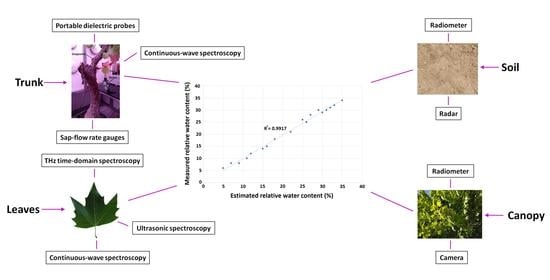
:This paper reviews the different remote sensing techniques found in the literature to monitor plant water status, allowing farmers to control the irrigation management and to avoid unnecessary periods of water shortage and a needless waste of valuable water. The scope of this paper covers a broad range of 77 references published between the years 1981 and 2021 and collected from different search web sites, especially Scopus. Among them, 74 references are research papers and the remaining three are review papers. The different collected approaches have been categorized according to the part of the plant subjected to measurement, that is, soil (12.2%), canopy (33.8%), leaves (35.1%) or trunk (18.9%). In addition to a brief summary of each study, the main monitoring technologies have been analyzed in this review. Concerning the presentation of the data, different results have been obtained. According to the year of publication, the number of published papers has increased exponentially over time, mainly due to the technological development over the last decades. The most common sensor is the radiometer, which is employed in 15 papers (20.3%), followed by continuous-wave (CW) spectroscopy (12.2%), camera (10.8%) and THz time-domain spectroscopy (TDS) (10.8%). Excluding two studies, the minimum coefficient of determination (R2) obtained in the references of this review is 0.64. This indicates the high degree of correlation between the estimated and measured data for the different technologies and monitoring methods. The five most frequent water indicators of this study are: normalized difference vegetation index (NDVI) (12.2%), backscattering coefficients (10.8%), spectral reflectance (8.1%), reflection coefficient (8.1%) and dielectric constant (8.1%).
1. Introduction
Water is one of the most important factors that have a significant influence on crop production. There is a direct relationship between biomass production and water consumed through transpiration [1]. Analyzing specific parts of a plant, leaf water content (LWC) is a crucial indicator of essential physiological processes [2], such as stomatal conductance (gs), transpiration, photosynthesis and respiration [3], which is closely related to forest fire ignition and fire propagation [4]. Furthermore, irrigation currently represents the largest consumption of water on the planet, reaching about 20% of the total amount of consumed freshwater and two-thirds of the total amount destined for human beings [5]. In addition to these factors, climate change, which has been increasingly consolidated over the last decades, has induced water scarcity in many parts of the world, leading plants to live under extreme situations of water stress and, therefore, causing a reduction in crop yield [6]. Monitoring the plant water status at real-time allows control the irrigation schedule, avoiding water stress and losses.
In order to schedule the irrigation periods of a crop and its amount of water, it is necessary to estimate the hydration level of each plant. There are numerous techniques to monitor plant water status. The most traditional techniques, such as leaf water potential [7] and thermogravimetric measurements [8], have proved to be highly reliable, but they cannot be considered as remote sensing techniques and, therefore, go beyond the objective of this paper. Remote sensing methods can be classified under multiple criteria and, in this work, they have been categorized according to the part of the plant subjected to measurement. In this way, the different sensors used in the available literature can be applied to the soil [9,10,11,12,13,14,15,16,17], directly to the canopy [18,19,20,21,22,23,24,25,26,27,28,29,30,31,32,33,34,35,36,37,38,39,40,41,42] or to different organs of individual plants, such as leaves [43,44,45,46,47,48,49,50,51,52,53,54,55,56,57,58,59,60,61,62,63,64,65,66,67,68,69,70] or trunks and stems [71,72,73,74,75,76,77,78,79,80,81,82,83,84,85].
Methods that estimate soil moisture content (SMC) use radiometers [9,11,13,14,15], radars [10,11,12,13,15], global navigation satellite system-reflectometry (GNSS-R) instruments [16] and/or cameras [17] on board satellites, manned and unmanned aircraft, and/or unmanned aerial vehicles (UAV), commonly known as drones, operating in the microwave, infrared (IR) and/or visible (VIS) range. The remote sensing data provided by these sensors include radiometer brightness temperature (TB), radar backscattering coefficients (σ) and remote images used to calculate specific indices related to moisture content, such as the normalized difference vegetation index (NDVI) [13,14,15], the vegetation water content (VWC) [13], the enhanced vegetation index (EVI) [13], the perpendicular drought index (PDI) [14], the temperature vegetation dryness index (TVDI) [14] and other indices based on the red, green and blue visible bands [17].
Concerning the approaches that estimate canopy water content (CWC), in addition to the same sensors used to monitor SMC (i.e., radiometers [18,19,20,21,22,23,24,25,26,27], radars [28], GNSS-R instruments [29] and/or cameras [26,30,31,32,33,34,35]), other remote inspection devices have been adopted, such as near infrared (NIR) and short wave infrared (SWIR) lasers under the terrestrial laser scanning (TLS) technique [36,37,38], portable [39] or mounted on manned aircraft [40,41] spectrometers operating in the visible and infrared spectrum, and a microwave rotating pencil-beam scatterometer installed on the International Space Station (ISS) [42]. In relation to the remote sensing data of these sensors, as in the case of soil moisture detection, brightness temperature, backscattering coefficients and spectral reflectance (Rλ) values are measured to obtain remote sensed indices correlated with the amount of water contained in the canopy. The most frequent vegetation indices used to estimate CWC or other physiological variables related to it, such as LWC, VWC, leaf area index (LAI), equivalent water thickness (EWT) and different crop water stress indices, are normalized difference infrared index (NDII) [18,24,37,38,40], NDVI [20,24,30,40], normalized difference water index (NDWI) [20,25,39,40,41] and canopy temperature [27,32,33,34,35].
Approaches applied to leaves can be categorized into destructive techniques [43,44,45,46,47,48,49,50,51,52,53,54,55,56], in which the leaves under test are detached from the plant before measurement, and non-destructive techniques [57,58,59,60,61,62,63,64,65,66,67,68,69,70], where remote sensing measurements are conducted directly on the plant. Most of the methods applied to individual leaves are contactless, with few exceptions [46,47,48,64,69,70]. The main sensors used to monitor the LWC comprise different spectroscopy techniques, such as terahertz (THz) time-domain spectroscopy (TDS) [43,44,45,57,58,59,60,61,62], THz quasi time-domain spectroscopy (QTDS) [61], continuous-wave (CW) spectroscopy [46,47,48,55,64,65,66], Fourier transform infrared spectroscopy (FTIR) [49], portable spectrometers [48,50,67] and air-coupled broadband ultrasonic spectroscopy [51,52,53,54,55,56], frequency-modulated continuous-wave (FMCW) radars [68] and porometers estimating gs [69,70]. In addition, these sensors estimate LWC through monitoring other parameters, such as reflection (Γ), transmission (T) and absorption (δ) coefficients directly correlated with LWC or used to calculate resonance frequencies [51,52,53,54,55,56,64] or specific spectral indices (i.e., moisture stress index (MSI) [50], ratio of thematic mapper band 5 to band 7 (TM57) [50], leaf water index (LWI) [50,67], simple ratio water index (SRWI) [50], the product between leaf optical depth (τ) and leaf surface area (LA) [58,59] and NDVI [67]) that also agree with LWC.
CWC can be also estimated by monitoring the water content of trunks or stems. Several studies use invasive methods to monitor CWC, consisting in the insertion of needles or probes inside the trunk or stems [71,72,73,74,76,81]. It is noteworthy to highlight that these approaches cannot be strictly considered as remote sensing techniques in spite of their widespread use in this research field. Other studies describe methods that need contact with the trunk or stems to develop the monitoring function [75,78,79,80]. Among the main sensors that estimate the tree water status include coaxial probes called portable dielectric probes (PDP) [71,72,73,74,75], volumetric soil water content (VSWC) sensors inserted into tree trunks [76], sap-flow measurements based on sensors that measure sap-flow rate (SFR) (g·h–1) [78,79,80] or sap-flux density (SFD) (m3·m–2·h–1) [77,81], CW vector network analyzer (VNA) spectroscopy [82,83], portable low-power cost-effective FMCW radars [84] and portable nuclear magnetic resonance (NMR) sensors [85]. In relation to the parameters measured by these sensors, PDPs, by using the complex reflection coefficient, estimate the complex xylem dielectric constant (XDC) to be correlated with the xylem SFD, the xylem sap chemical composition and xylem water potential (XWP). The VSWC sensors estimate XDC to be correlated with the stem water potential (SWP). Sap-flow measurements constitute an estimation of the tree water status. The most widely used techniques in order to measure sap-flow rate and SFD are the heat balance (HB) [78,79,80] and the heat pulse (HP) [77,81] methods. CW-VNA spectrometers measure the trunk reflection coefficient correlated with the VSWC (humidity probe) and with the trunk diameter variation measured by a dendrometer. Portable FMCW radars acquire the signal reflected by the xylem tissue to be correlated with the VSWC. Finally, NMR sensors measure the amplitude of the NMR signal, which scales linearly and quantitatively with the total amount of water contained within the sensor.
In this paper, we reviewed the different remote sensing techniques and approaches found in the literature, as well as their applications, for assessing plant water status. The scope of this paper covers a broad range of 77 scientific works published between the years 1981 and 2021, including mostly journal papers and some books and conference proceedings, and collected from different search web sites, especially Scopus. Different technologies and sensors used to conduct remote sensing are described in Section 2. Section 3 introduces the most relevant results of the collected references. Section 4 presents the discussion of results. Finally, Section 5 concludes this paper.
2. Sensors and Techniques
Throughout the review process, a wide variety of passive and active sensors used to monitor plant water status have been identified. Passive sensors measure radiation reflected by the tested object coming from a source different from the instrument or emitted by the object itself. Sunlight is the most frequent source of radiation detected by this type of devices. The most typical passive sensors include radiometers and spectrometers mounted on satellites and aircraft, cameras and portable spectrometers. Conversely, active sensors illuminate the object with their own electromagnetic radiation and then measure the radiation that is reflected, backscattered or transmitted through this object. The most common active sensors are radars, lasers, scatterometers, VSWC probes, PDPs, SFR and SFD gauges and some kinds of spectroscopy techniques, such as THz-TDS, THz-QTDS, CW spectroscopies, FTIR spectroscopy and air-coupled broadband ultrasonic spectroscopy. In the case of ultrasonic spectroscopy and sap-flow measurements, the electromagnetic radiation is replaced by acoustic waves and thermal energy respectively. In the following subsections, the most relevant sensors collected in this paper are briefly outlined.
2.1. Radiometer
This is an instrument that measures the radiant flux emitted or reflected by a given object and usually works in a portion of the spectrum selected among the visible, infrared or microwave bands [86]. Sometimes, it covers multiple bands simultaneously and is called multichannel radiometer. Satellites and manned aircraft are typically used as platforms.
In the case of microwave radiometers, it is very common to express the power in terms of an equivalent temperature, called brightness temperature (Figure 1) and defined as the physical temperature of a blackbody that would radiate the same power at the considered wavelength. The output of a microwave radiometer is actually a voltage value proportional to its antenna temperature (TA) and the final goal of the measurement is to relate this antenna temperature to the brightness temperature of the object [87]. In the literature, different methods to retrieve SMC and VWC on the basis of TB have been found, such as the direct correlation between water content and TB [9] or TB normalized by the land surface temperature [9], the calculation of specific indices sensitive to water content [9,19,22], the application of retrieval models [18,23] and the implementation of decision-making algorithms [21].
Regarding radiometers operating in the infrared and visible ranges, all the devices found in the literature are imaging radiometers, which include the scanning capability to provide a two-dimensional array of pixels for producing an image. They are often called imagers or scanners, and the scanning can be carried out mechanically or electronically by using an array of detectors [86]. From the obtained images, imaging radiometers allow the measurement of the radiance in a specific direction towards the object or under a specific angle of view and, finally, the calculation of the reflectance in order to obtain the suitable spectral indices.
A large number of terms are usually used to describe the same type of radiometer leading to confusion. In this work, the following criterion has been followed: when the device operates in a single frequency band, it is simply called radiometer, for instance, the radiometer on board the soil moisture active passive (SMAP) satellite at 1.41 GHz [23]; when it works in several discontinuous frequency bands of bandwidth larger than approximately 10 nm, multichannel or multispectral radiometer is the term used to define it. Most multispectral radiometers have four basic spectral bands, such as blue, green, red, and NIR bands. Some of them have additional spectral bands in the SWIR and thermal infrared (TIR) regions of the spectrum. Two examples of this kind of scanner are the operational land imager (OLI) and the thermal infrared sensor (TIRS) on board the Landsat-8 satellite [14,26]; finally, when the instrument is designed to obtain imagery over hundreds of narrow and continuous spectral bands with typical bandwidths of 10 nm or less, it is called hyperspectral radiometer or spectrometer, which is described in the following subsection.
2.2. Spectrometer
It is a device that detects, measures and analyzes the spectral content of the incident electromagnetic radiation. Conventional imaging spectrometers use gratings or prisms to discriminate the spectral content on the basis of its wavelength [86]. The spectrometers collected in this paper are of two types: imaging spectrometers mounted on manned aircraft, such as airborne visible/infrared imaging spectrometer (AVIRIS) [40] and airborne visible/infrared imaging spectrometer-next generation (AVIRIS-NG) [41], and portable spectrometers.
Imaging spectrometry consists in the acquisition of images in hundreds of contiguous spectral bands such that for each pixel a radiance spectrum or spectral radiance measured in W·sr−1·m−2·nm−1 can be derived [88]. Imaging spectrometers are designed to measure the spectral radiance coming from an object as a function of two spatial and one spectral dimension, that is, a 3-D dataset usually called data cube. Afterwards, from these radiance values, the reflectance in each pixel is obtained in order to calculate the required spectral indices. Figure 2 shows the data cube provided by a spectrometer under the hyperspectral imaging technique. The third dimension in the cube represents the spectral content of each pixel.
Hyperspectral sensors divide the spectrum into several narrow spectral bands, instead of a single wide band. On account of this, these instruments can provide high resolution spectral information from the object. However, a reduction in the width of the spectral bands also means a reduction of the signal received by the sensor. With the objective of maintaining a specific signal-to-noise ratio (SNR), the pixel size has to be enlarged and the spatial resolution decreases, leading to a trade-off between spatial and spectral resolution. In order to improve the spatial resolution of the images, airborne imagery is usually adopted [90]. Remote sensing imaging spectrometers may be categorized by the method they use to achieve the spatial and spectral discrimination. Whiskbroom, pushbroom, framing and windowing are the main techniques to discriminate the spatial information, while filtering, dispersive and interferometric techniques are the most commonly used methods to obtain the spectral discrimination [88,91,92].
Additionally, portable spectrometers that estimate the water content of leaves with destructive and non-destructive techniques are widely used in the reviewed literature because they allow the user to transport the instrument from the laboratory to the sample, instead of taking the sample to the spectrometer. There are different types of portable spectrometers, such as optical or molecular spectrometers, elemental spectroscopy, mass spectrometry (MS), portable gas chromatography-mass spectrometry (GC-MS), ion-mobility spectrometry, NMR spectrometers, small electron spin resonance (ESR) instruments and millimeter wave spectrometers among others [93]. The spectrometers collected in this review are optical covering the visible, NIR and SWIR spectral bands.
2.3. Camera
Over the last decade, UAVs, also known as drones, unmanned aircraft systems (UAS) or remotely piloted aircraft systems (RPAS), have been increasingly employed. Recent studies have indicated that the application of these devices is revolutionizing a large number of research areas, such as forestry studies, spatial ecology, ecohydrology and other fields related to environmental monitoring. This revolution has been possible thanks to the technological progress and miniaturization of sensors, airframes, and software. UAV sensing technology has enabled scientists to obtain custom cost-effective imagery at high spatial resolution ranging from 1 cm to 1 m. Before UAVs were consolidated, external companies or institutions were the responsible entities for providing datasets by means of the utilization of sensors mounted on satellites and manned aircraft. Nowadays, research groups purchase or build their own remote sensors without the support of these entities. Although UAV remote sensors are not very different from those on board satellites and manned aircraft, small differences may exist in performance, data processing, calibration, spatial and spectral resolution, measurement geometries and measurement timings [94].
In the heart of this miniaturization, cameras have burst onto the scene as devices combined with UAVs to monitor plant water content. The four types of cameras found in the literature covered by this review are conventional RGB, multispectral, hyperspectral and TIR cameras. A conventional digital camera possesses an image sensor that converts electromagnetic energy into electrical charges. Although the image sensor in most digital cameras is a charge-coupled device (CCD), some of them use complementary metal oxide semiconductor (CMOS) technology. Its spectral range is limited to the three visible bands, that is, red, green and blue bands, and it automatically combines the spectral bands into an image [95]. Multispectral and hyperspectral cameras are the miniaturized devices analogous to the multispectral imaging radiometers and hyperspectral spectrometers respectively, explained in the two previous subsections. Similarly to these devices, the multispectral and hyperspectral cameras of this review operate in the VIS/IR frequency range. Finally, TIR cameras are described in the following subsection.
2.4. Thermal Remote Sensors
This type of sensors measure the radiation emitted by an object due to its thermal state, instead of measuring the radiation reflected by the object after being illuminated by solar radiation. All objects with a temperature higher than the absolute zero (−273.15 °C) emit electromagnetic radiation. Due to the infrared atmospheric windows, thermal remote sensors usually operate in the 3–5 μm and 8–14 μm frequency ranges [86]. In the particular case of this review, all the used thermal sensors operate in the second range of 8–14 μm.
The thermal infrared sensors collected in this review are TIR radiometers [9,27], which have already been described in Section 2.1, conventional portable infrared thermometers [27] and TIR cameras. A TIR camera is a device similar to a conventional RGB camera but with a spectral range of approximately 7.5–13.5 μm. Figure 3 shows the simplified crop water stress index (CWSIsi) of a cotton field, which is estimated on the basis of the cotton canopy temperature measured by a TIR camera on board a drone. Its calculation procedure is detailed in Section 3.2.
2.5. Radar
It is an electromagnetic sensor, usually in the range of microwave frequencies, used to detect the position, distance and velocity of an object from the radar placement. It consists in radiating electromagnetic energy towards the object and monitoring the reflected signal from it [86]. Depending on the type of signal used to monitor the object, radars can be categorized into two main groups: continuous-wave (CW) and pulsed radars. Specifically, the sensors found in this review are synthetic aperture radars (SAR) mounted on satellites (Figure 4a) and manned or unmanned aircraft, which use pulsed waveform, and frequency-modulated continuous-wave (FMCW) radars (Figure 4b).
2.5.1. Synthetic Aperture Radar
SAR systems, such as the C-band SAR on board the Sentinel-1 satellite, were created in an attempt to improve the spatial resolution at long distances. For a real aperture radar system, the minimum dimension of an object that can be detected (Rs) is calculated as [97]:
where λ is the wavelength, h is the height of observation and ϕ is the diameter of the antenna. Therefore, when the height of observation reaches a considerable value, as in space platforms, achieving a suitable resolution would require using a very large antenna. This limitation can be overcome by using an artificially synthesized virtual antenna that is the fundamental concept of SAR systems. Doppler effect, namely the change in the frequency of the received signal as a result of the relative movement between the sensor and the observed object, is used to synthesize the adequate antenna and obtain high-resolution image data of the surface under test [97]. SAR technology features relevant characteristics compared to other imaging techniques used in remote sensing. Firstly, as happens with other technologies, such as microwave radiometers, radars, scatterometers and thermal sensors among others, it enables the monitoring of the Earth’s surface independently of the natural light, that is, at night or on cloudy days. Another important advantage of SAR technology is the penetration capacity that allows the penetration into vegetation to estimate the SMC beneath the canopy at different depths. The specific parameters used to monitor the soil and canopy moisture content are the backscattering coefficients, which depend on specific physical properties of the observed surfaces, such as the dielectric constant (ε), closely related to their amount of water. Each pixel of an image obtained by means of radar imaging represents the backscattering coefficient of that area on the ground that reflects the electromagnetic energy, and the greater the stored value, the more intense the received signals will be [97].
2.5.2. Frequency-Modulated Continuous-Wave Radar
FMCW radars emit continuous radio frequency (RF) power during the measurement, changing their operating frequency by means of a frequency synthesizer that offers several modulation ramps. This type of sensor divides the transmitted power into two signals, the reference signal used as local oscillator (LO) and the RF signal, which is radiated toward the target, reflected, and sent back to the receiver to be mixed with the reference signal. At the mixer input, the time delay between both signals can be estimated from their frequency difference and used to determine the distance D to the reflecting object by applying the following equation [84]:
where c is the speed of light in vacuum, Δf is the frequency difference measured between both signals, Tr is the modulation wave period or ramp time, and BW is the bandwidth of the transmitted signal. For a medium different from vacuum, c must be replaced by the group velocity Vg at which the electromagnetic wave propagates in the medium. The depth resolution ΔD, defined as the minimum separation in depth between two targets of equal cross section that makes it possible to identify them as separate targets, can be expressed as follows [84]:
The application of this technology on the monitoring of plant water content consists in measuring the power reflected on the plant for different degrees of hydration. The part of the plant more commonly subjected to measurement is its trunk [84].
2.6. Scatterometer
It is a side-looking radar sensor designed to measure σ with high radiometric resolution at the cost of sacrificing spatial resolution [98]. Radiometric resolution is the capacity of a detector to detect different input signal levels. The more sensitive the sensor, the higher the radiometric resolution is. Scatterometers are sensors complementary to SAR devices. These sensors, unlike scatterometes, optimize the spatial resolution at the expense of the radiometric resolution. Therefore, while satellite SAR systems are characterized by a spatial resolution of about 1 m, with a low radiometric resolution related to the speckle noise, satellite scatterometers have a spatial resolution of about 10 km, with a radiometric resolution to measure σ within a tenth of a decibel. Although these remote sensors were initially designed to estimate the speed and direction of wind across ocean surfaces, its use has also been extended to monitor continental surfaces. One of the applications of this continental monitoring, which has been included among the different collected references [42], is the vegetation water stress detection. The application of this technology on the monitoring of plant water content is very similar to SAR technology, consisting in the measure of the backscattering coefficients of the observed surfaces.
2.7. Terrestrial Laser
The monitorization of CWC by means of laser devices is mainly based on the terrestrial laser scanning (TLS) technology, also referred to as terrestrial light detection and ranging (LiDAR) or topographic LiDAR. This technology measures range (XYZ coordinates) and reflectance of the surface points of the object under test after emitting laser pulses toward them. Modern TLS devices, such as Leica P20, P40 and P50 (Leica Geosystems, Heerbrugg, Switzerland) can measure about 106 points per second with an accuracy lower than 1 mm within a range of 10 m (Figure 5a). Lidar instruments can be mounted on a tripod over the ground in order to capture the shape of objects in the surrounding (TLS technology), or placed on moving platforms such as aircraft, helicopters, cars or vessels. If the scanning instrument is placed on board a flying platform, the technology is called airborne Lidar or airborne laser scanning. On the contrary, if the laser is mounted on a car, van or boat, the technology is referred to as mobile laser scanning, terrestrial mobile mapping or, more commonly, mobile mapping [99]. The technology more frequently used in order to estimate the water status of a plant by means of laser devices is TLS. The found references related to this technology are based on the NDII calculation of individual leaves and on the subsequent correlation of these NDII values with EWT, which is the amount of water in leaf per unit leaf surface area. Once this model is created and validated, different trees in their entirety are monitored in order to obtain NDII point clouds and, therefore, using the model, EWT point clouds (Figure 5b) [37,38].
2.8. Soil Moisture Sensors
There are basically two types of soil moisture sensors: those that measure the soil water potential, such as tensiometers and granular matrix sensors, and those based on dielectric techniques that measure VSWC. Tensiometers measure the soil matric potential by means of a porous tip, that is, the suction pressure required for a plant to obtain water from the soil. Granular matrix sensors measure the electrical resistance between two electrodes in a porous matrix, which is a function of the soil matric potential [100,101]. Concerning the dielectric techniques, they can be divided into time-domain and frequency-domain approaches. Time domain reflectometry (TDR) estimates the apparent permittivity of the soil by measuring the propagation time of a pulsed electromagnetic signal along a waveguide consisting of two or three parallel rods. The time the wave takes to reach the end of the waveguide and back is directly related to the dielectric properties of the soil and, therefore, to its soil moisture content [102]. Time domain transmissiometry (TDT) is a variant of TDR that measures the transmission time, instead of the reflection time, of a pulse along a transmission line consisting of a looped rod. As with TDR, there is no complex waveform analysis [103]. In the case of the techniques based on the frequency domain, two types of approaches can be adopted: frequency domain reflectometry (FDR) and capacitance sensors. Although FDR sensors, as in the case of TDR, are constituted by a waveguide composed of two or three parallel rods, a frequency-swept signal is transmitted along the waveguide. Depending on the type of FDR sensor, some establish a relationship between permittivity and resonance frequency and others relate permittivity with reflection and transmission coefficients. Unlike TDR, FDR enables the estimation of the complex dielectric constant. Finally, capacitance techniques estimate the soil dielectric constant by measuring the charge time of a capacitor that uses the soil as the dielectric material between its conductors [102].
The use of soil moisture probes in this review is clearly intended to provide ground-truth data in order to correlate this information with the one provided by the specific remote sensing technique. Only a few VSWC sensors have been used as the main sensing technique to monitor plant water content. This is the case of commercial VSWC sensors inserted into tree trunks (Figure 6) [76] or a type of FDR sensor specially designed to monitor the xylem water content inside the trunk [71,72,73,74,75]. This last approach, called PDP, is based on open-ended coaxial probes at microwave frequencies that measure the complex reflection coefficient at the end of the semirigid transmission line. The xylem water content is estimated by means of the relationship between the magnitude and phase of Γ and the complex dielectric constant of the medium at the probe tip.
Concerning the use of soil moisture sensors as tools to provide ground-truth data, it is worth highlighting the soil moisture sensing controller and optimal estimator (SoilSCAPE) network [104] developed to measure soil moisture at a high temporal resolution by using a combination of wireless sensor networks and soil sensors. SoilSCAPE has been widely used in the calibration/validation of many satellite missions.
2.9. Sap-Flow Rate and Sap-Flux Density Gauges
A review of the literature on this kind of sensors has allowed the identification of different methods to carry out sap-flow measurements. These sensors are based on the application of heat in the sapwood, which is transported by the moving sap. Thanks to this movement, sap flow can be estimated by monitoring temperature changes around the heater. The first classification of these measurement devices can be made between those that measure the total sap flow in a plant stem or stem section, which is called sap-flow rate (SFR) (g·h–1), and those that measure the amount of sap passing through a specific surface per unit of time, which is called sap-flux density (SFD) (m3·m–2·h–1) [77].
Among the SFR approaches, it is possible to distinguish the stem heat balance (SHB) and trunk sector heat balance (THB) methods. The SHB method can be used in both woody and herbaceous stems as small as about 4 mm in diameter. Commercial heat balance gauges can fit stems of diameters ranging from 2–125 mm. The SHB technique uses a flexible heater wrapped around the stem and, in turn, enclosed in a layer of cork. These two layers are covered by two others, a layer of foam insulation and an outer weather-resistance shield. By measuring the radial (between the inner and outer cork surfaces) and axial (above and below the heater) temperature gradients by means of thermocouples and applying the heat balance to the stem by means of these temperature gradients, the mass flow rate of sap is calculated in g·h–1 [105]. The THB method is used in tree trunks with diameters larger than 120 mm. As in the previous method, the heat balance is applied to a trunk sector. However, rather than superficially spherical, the heat is applied internally using five stainless steel electrode plates inserted into the wood. Using four thermocouples inserted into the sapwood and positioned at the same height as the plates, and four other thermocouples 100 mm below, it is possible to apply the heat balance in order to estimate the mass flow rate of sap [105].
SFD techniques can be divided into continuous heat SFD methods and heat-pulse SFD methods. Continuous heat approaches relate SFD to a temperature difference measured between a constantly heated needle and different unheated needles intentionally inserted in specific positions around the first one. Thermal dissipation (TD) and heat field deformation (HFD) methods are the most important continuous techniques [77]. In the heat-pulse method, short pulses of heat are applied by means of a needle inserted in the sapwood and the sap-flux density is calculated by measuring the propagation velocity of the heat pulses along the stem. The most relevant heat-pulse techniques are compensation heat-pulse velocity (CHP), Tmax, heat ratio (HR), calibrated average gradient (CAG) and sapflow+ among others [77]. A limitation of heat-pulse approaches is that they need to be applied to stems with diameters large enough to be able to accommodate the measurement needles. The smallest stem diameters found in the literature range from 5–6 mm [81].
2.10. Electromagnetic Spectroscopy
Spectroscopy is the study of the interaction between matter and electromagnetic radiation as a function of the wavelength. Currently, there are different spectroscopy techniques depending on their particular application. The most relevant spectroscopy techniques used to estimate plant water status are: terahertz time-domain spectroscopy (THz-TDS), terahertz continuous-wave (THz-CW) spectroscopy, terahertz quasi time-domain spectroscopy (THz-QTDS), continuous-wave vector network analyzer (CW-VNA) spectroscopy and Fourier transform infrared (FTIR) spectroscopy. Table 1 presents a summary of the different electromagnetic spectroscopy techniques used in this review, including the setup components, if the generated signal is pulsed or continuous and the operating frequency.
2.10.1. Terahertz Time-Domain Spectroscopy
The operating principle of THz-TDS is to generate periodic femtosecond pulses of electromagnetic radiation by means of a photoconductive antenna that acts as the system transmitter and to receive these pulses after passing through the sample by using another photoconductive antenna that acts as the system receiver [106]. The properties of the sample can be estimated by comparing the results between the sample measurement and the reference measurement. The reference measurement, which is carried out for each sample, consists in performing a measurement between the transmitter and receiver without the sample to record the characteristics of the measurement setup. Once the measurement has been completed, it is possible to obtain its frequency dependence by applying the Fourier transform (FT) to the time-domain data [61]. The central component of the THz-TDS is a laser, which emits femtosecond pulses of light. These short pulses are used to excite the photoconductive antennas of the transmitter and receiver. At the transmitter antenna, by means of the application of a static bias voltage to the antenna semiconductor, the photo-excited carriers are accelerated giving rise to short radiated THz pulses. The detection of these pulses is performed by an unbiased photoconductive antenna simultaneously excited by the laser pulses that generate free carriers in the semiconductor material. These carriers are accelerated by the THz incoming electric field generating a photocurrent that feeds a transimpedance amplifier followed by a lock-in amplifier [61,106,107].
2.10.2. Terahertz Continuous-Wave Spectroscopy
THz-CW spectroscopy uses a similar setup to the one of THz-TDS, but the photoconductive antennas are excited by a CW laser beam, instead of light pulses. This beam is the result of photomixing two laser beams slightly detuned against each other. When the photoconductive antenna of the transmitter is excited by this optical signal, a THz radiation at the difference frequency of the two lasers is generated. Similar to THz-TDS, the amplitude of the THz signal after passing through the sample is an indicator of the plant water status. The development of this spectroscopy technique by means of photomixing has the advantage of generating a THz beam with high spectral resolution. This mixing process provides a quasi-monochromatic THz beam, whose bandwidth could be less than 1 kHz. This technique is particularly appropriate when the required frequency band must fit the specific absorption line of the samples under test [61,106].
2.10.3. Terahertz Quasi Time-Domain Spectroscopy
THz-QTDS setup is almost identical to the one of THz-TDS, but replacing the femtosecond laser by a cheap multimode laser diode. Since a laser diode can generate light at different wavelengths simultaneously, it is possible to make use of a large number of difference frequencies by using only one multimode laser diode, unlike THz-CW spectroscopy, which is performed with two CW lasers. The final result is a signal that looks like a train of THz pulses. This similarity with the THz-TDS time-domain waveform is where the name quasi time-domain spectroscopy comes from. The main objective is to achieve a spectroscopy technique similar to THz-TDS, but more compact and cost-effective [61].
2.10.4. Continuous-Wave Vector Network Analyzer Spectroscopy
CW-VNA spectroscopy makes use of a vector network analyzer, apparatus that provides the scattering parameters of the sample under test for a large bandwidth. This spectroscopy technique works at microwave and terahertz frequencies. Generally, a CW signal at microwave frequency is generated by a microwave source included in the VNA. This signal is multiplied by nonlinear diodes (e.g., Schottky diodes) in order to convert it up to higher microwave or terahertz frequencies. These nonlinear diodes used to perform the frequency upconversion are included in modules called VNA extenders. Finally, by means of an antenna, attached at the end of the extender waveguide, the beam is directed toward the antenna of the receiver extender after passing through the sample. At the receiver, a downconversion process reverse to the previous one is carried out. High dynamic range (higher than 100 dB), high spectral resolution (sub-kHz for the best systems) and large bandwidth are the main advantages of this spectroscopy technique. On the contrary, the need for a precise calibration, its upper frequency limit and the possible appearance of the standing wave effect between the antennas are the most relevant drawbacks [106].
2.10.5. Fourier Transform Infrared Spectroscopy
FTIR spectroscopy is based on the Michelson interferometer, consisting in a polychromatic infrared source, a beam splitter, a fixed mirror and a moving mirror (Figure 7) [106]. The beam splitter is designed to transmit half of the incident light toward the moving mirror and to reflect the other half toward the fixed mirror. The fixed and moving mirrors reflect the radiation back to the beam splitter. Again, half of this reflected radiation is transmitted and half is reflected at the beam splitter. Due to these second reflections, two light beams will appear at the detector path, which are recombined into a single light beam that leaves the interferometer, interacts with the sample and strikes the detector. The optical path difference (OPD) between the two beams due to the displacement of the moving mirror results in interference patterns. For instance, for a specific wavelength, depending on the mirror position, the interference between both beams will be constructive or destructive. When this recombined light beam passes through the sample, a part of the radiation at certain frequencies is absorbed by it and does not reach the detector. Therefore, the final interferogram is composed of all frequencies except for those absorbed by the sample. Finally, in order to convert the OPD-dependent raw data into a frequency-dependent function, the Fourier transform is applied.
2.11. Air-Coupled Broadband Ultrasonic Spectroscopy
The development of new broadband ultrasonic transducers, capable of working in gaseous media (air-coupled transducers), has enabled the application of this spectroscopy technique to the measurement of materials without the need to use any coupling fluid to attach the transducer to the surface of the material [55]. The experimental setup (Figure 8) consists of two specially designed air-coupled piezoelectric transducers operating at MHz frequencies and positioned facing each other at a distance of a few centimeters (approximately 0.3–1.2 MHz and 2 cm for the measurement of LWC). A high voltage (100–400 V) microsecond pulse is applied to the transmitter transducer, which converts it into an ultrasonic pulse that propagates through the air. Passing through the sample, the ultrasonic signal reaches the receiver transducer, which converts it into an electrical one again. Then, it is amplified and filtered (typically a low-pass filter at 10 MHz). Finally, an oscilloscope digitizes this electrical signal, averages several waveforms to reduce the high frequency noise and applies the fast Fourier transform (FFT) transferring the data to a computer. Before performing the measuring process, a measurement without the sample is carried out in order to calibrate the setup. Afterwards, the final measurement is performed by positioning a leaf between the transducers for a few seconds at normal incidence. From this measurement, the magnitude and phase of the transmission coefficient is obtained in the frequency domain. In the particular case of LWC estimation, other parameters, such as the standardized thickness resonance frequency (f/f0), the quality factor of this thickness resonance (Q), the macroscopic effective elastic constant in the leaf thickness direction (c33), the attenuation coefficient (α) and the variation of the attenuation coefficient with the frequency (n), are calculated on the basis of this transmission coefficient and correlated with the RWC. In relation to the f/f0 parameter, f represents the frequency value associated with the maximum transmittance for any RWC value of a leaf and f0 is the frequency value at which the maximum transmittance is reached when RWC = 1. Although this spectroscopy technique is a non-destructive and non-invasive approach, all references found in the literature that monitor RWC of leaves by means of this technique make use of leaves detached from the plant instead of in-vivo measurement. For this reason, these references have been classified in this work as destructive approaches.
2.12. Global Navigation Satellite System Reflectometry
The most common configuration of a GNSS-R system is the same as that used by a bistatic radar. It consists in measuring the direct and reflected GPS signals by means of right-hand (RHCP) and left-hand (LHCP) circularly polarized antennas respectively. The direct signal is used to calibrate the system and the reflected signal contains information about the Earth’s surface. One important application of this technology is the assessment of SMC and VWC from ground-based [29,110], airborne [16] and spaceborne [111] platforms.
3. Different Approaches Based on Targets
This section presents a brief description of the most relevant approaches on monitoring of plant water content found in the literature. Results are presented according to the part of the plant subjected to measurement, namely, soil, canopy, leaves or trunks. Moreover, approaches applied to leaves are divided into destructive techniques, in which the leaves under test are detached from the plant before measurement, and non-destructive techniques, in which the remote sensing measurements are carried out in-vivo in the plant itself. Concerning the monitoring techniques applied to trunks or stems, they are separated considering invasive approaches that make use of probes, needles and electrodes inserted in the sapwood, and non-invasive approaches, which monitor the plant water status remotely by means of a sensor.
3.1. Soil Techniques
The approaches found in the literature that try to estimate SMC [9,10,11,12,13,14,15,16,17] use radiometers [9,11,13,14,15], radars [10,11,12,13,15], GNSS-R instruments [16] and/or cameras [17] on board satellites, manned and unmanned aircraft, and/or UAVs, commonly known as drones, operating in the range of microwave, infrared and/or visible. Table 2 shows a summary of the references that use soil techniques in this review including the indicator used to estimate the water content, the indicator operating frequency, the fitting curve used between the estimated and measured data, the coefficient of determination (R2), the estimation error, the employed technology, the target or part of the plant under test and the platform used by the sensor to develop the monitoring function.
When radiometers are the remote sensors chosen to monitor SMC, satellites [13,14,15] and manned aircraft [9,11] are the most common platforms. Radiometers on board manned aircraft usually work at microwave frequencies and use the brightness temperature in order to obtain a SMC map of the area under study. Fang et al. [11], in addition to an L-band (1.413 GHz) radiometer mounted on a manned aircraft, use a high-resolution L-band (1.26 GHz) SAR mounted on an unmanned aircraft. By means of a soil moisture disaggregation algorithm that integrates soil moisture retrievals provided by the radiometer and high-resolution observations provided by the radar, it is possible to achieve soil moisture estimates at a finer scale. For a spatial resolution of 800 m, the estimated SMC is well correlated to the in-situ soil moisture measurements with a coefficient of determination (R2) ranging from 0.628 (1.5 Kg/m2 ≤ VWC ≤ 2.5 Kg/m2) to 0.794 (VWC ≥ 2.5 Kg/m2) accompanied by an unbiased root mean square error (RMSE) ranging from 0.025 to 0.091 m3/m3. Macelloni et al. [9] make use of two radiometers on board an ultra-light manned aircraft, a multichannel microwave radiometer at L (1.4 GHz), C (6.8 GHz) and X (10 GHz) bands, and a thermal infrared radiometer (8–14 μm) to normalize TB by the thermal infrared temperature of the surface. For the case of bare soils, the correlation coefficient (R) of the linear regression model between the estimated and ground measured SMC at L band reaches a value of 0.84 with a standard error of estimate (SEE) of 3%. In addition, an experimental study for estimating the SMC at different depths was carried out by those authors revealing a strong sensitivity of L band to SMC within a layer of 5 cm regardless of the surface roughness, and of X band to SMC within a layer of 2.5 cm on smooth surfaces. The correlation coefficients of the linear regression models between the normalized brightness temperature (TN) and ground measured SMC at L and X bands are 0.94 and 0.8 respectively. Huang et al. [13] conduct a soil moisture retrieval model combining two satellite sensors, the Sentinel-1 C-band SAR to estimate the SMC and the Landsat-8 VIS/IR OLI to eliminate the influence of the vegetation canopy on the radar backscattering coefficients by means of three vegetation indices: NDVI, VWC and EVI. The highest coefficient of determination between the estimated and in-situ soil moisture is 0.76 (RMSE = 2.04%), which is reached under the VWC vegetation index. Wang et al. [14] provide two combination approaches of the PDI and TVDI indices, the joint model and the combined model. These indices are calculated on the basis of the remote sensing data acquired from the Landsat-8 multichannel radiometers: OLI and TIRS. The RMSE of the joint/combined models between the estimated and ground measured SMC at different soil depths are: 1.49%/1.48% at 0–20 cm, 1.46%/1.48% at 0–30 cm and 1.86%/1.90% at 0–40 cm. Practically for all measurements, RMSE values of the joint and combined models are lower than the ones generated by the individual models. Tao et al. [15] propose an approach similar to the one of [14]. They developed a vegetation backscattering model to retrieve vegetation-covered SMC based on the backscattering coefficient of the RADARSAT-2 C-band SAR and field measurements. In this case, the vegetation scattering is estimated by using multichannel VIS/IR imaging radiometers, particularly four 16-m wide field imagers (WFI) on board the GaoFen-1 satellite that enable the calculation of the NDVI index. The best fit between the measured and estimated SMC features an R2 of 0.806 with an RMSE of 0.043 m3/m3.
Concerning the use of radars to monitor SMC, all the references except [10,12] have already been described previously. Eweys et al. [10] use the same SAR previously described in [15] to develop a cumulative distribution function (CDF) matching approach for quantifying the soil and vegetation contributions to the satellite signal. This is achieved by means of the comparison of two signals acquired at the same location when the soil is bare and covered with vegetation on the condition that both signals must have the same cumulative probability. The linear regression model between the measured and retrieved SMC in the presence of vegetation shows an R2 of 0.64 and an RMSE of 0.03 m3/m3. Chatterjee at al. [12] make use of the same SAR described in [13] to develop an empirical SMC retrieval model by combining the sensor data with multiple ancillary datasets (e.g., terrain, land cover, soil properties) and correlating the estimated SMC with field measurements performed at the United States Climate Reference Network (USCRN) stations within a layer of 5 cm. In terms of calibration, R2 = 0.941 (RMSE = 0.029 m3/m3) is the highest coefficient of determination achieved by one of the three developed models. In terms of validation, the coefficient of determination decreases to 0.676 with an RMSE of 0.065 m3/m3.
Regarding the use of GNSS-R instruments to estimate SMC, Munoz-Martin et al. [16] evaluate the reflectivity of the land surface by using an airborne-based microwave interferometer reflectometer (MIR) at L1 (1575.42 MHz) and L5 (1176.45 MHz) bands, and at different integration times. The soil moisture retrieval is obtained by applying an artificial neural network (ANN) to the reflectivity values. The ANN soil moisture data are correlated with a 20-m resolution downscaled estimation approach developed by combining the data of the soil moisture and ocean salinity (SMOS) mission together with the Sentinel-2 NDVI data and the European centre for medium-range forecast (ECMWF) land surface temperature. The maximum correlation coefficient (R = 0.99) is reached for an integration time of 5 s with a SEE value of 0.016 m3/m3.
In relation to the SMC estimation by using cameras, the collected approaches lack in accuracy. Putra and Nita [17] use aerial photography by means of a conventional digital camera on board a drone to calculate different spectral indices based on the red, green and blue bands. The results show that the correlation coefficient between the ground measured SMC and the RGB bands, the digital elevation model (DEM) and the different spectral indices is below 0.5, where the triangular greenness index (TGI) features the highest value (R = 0.32).
3.2. Canopy Techniques
Concerning the approaches aimed at estimating the CWC, in addition to the same sensors used to monitor the SMC (i.e., radiometers [18,19,20,21,22,23,24,25,26,27], radars [28], GNSS-R instruments [29] and/or cameras [26,30,31,32,33,34,35]), other remote inspection devices have been adopted, such as NIR and SWIR lasers under the TLS technique [36,37,38], portable spectrometers [39] or mounted on manned aircraft [40,41] operating in the visible and infrared spectrum, and a microwave rotating pencil-beam scatterometer installed on the ISS [42]. Table 3 shows a summary of the references that use canopy techniques in this review.
Hunt et al. [18] compare independent estimates of VWC between the Windsat polarimetric microwave multichannel radiometer on board the Coriolis satellite and the moderate resolution imaging spectroradiometer (MODIS), which is a multispectral VIS/IR imaging radiometer aboard the Terra and Aqua NASA’s satellites. Results show that there is a linear relationship between both estimates with an R2 = 0.82 and an RMSE = 0.96 Kg/m2. The spectral index used to estimate CWC by using MODIS and, in turn, VWC is NDII. Calvet et al. [19] use the Nimbus-7 scanning multichannel microwave radiometer (SMMR) temperature-corrected data at 6.6 and 37 GHz to derive the water status evolution of the Amazon forest canopy. For this purpose, and after applying atmospheric corrections to the data for water vapor, clouds and rain, the moisture ratio (MR) vegetation humidity index is defined and correlated with variations of stomatal resistance (R2 = 0.85 with RMSE = 10.91 s·m–1 for the wet season). Jackson et al. [20] map and monitor VWC for corn and soybean canopies by using two spaceborne multispectral VIS/IR imaging radiometers, the thematic mapper (TM) and the enhanced thematic mapper plus (ETM+) on board the Landsat-5 and Landsat-7 satellites respectively. From the obtained images, the NDVI and NDWI indices are calculated and mathematically related to VWC, calculated with gravimetric techniques at the different sampling fields. In relation to the validation of the mathematical models, the minimum RMSEs are obtained with the NDWI index with values for corn and soybean canopies lower than 0.576 and 0.171 Kg/m2 respectively. In addition, CWC estimation is a crucial factor for early detection of fire risk [21]. Thus, these authors develop a decision-making system in which the moisture of forest canopy is estimated by using the brightness temperature provided by the manned flying platform IL-18 equipped with microwave radiometers operating at 1.43, 13.3 and 37.5 GHz. Firstly, by means of a regional hydrological model, the low moisture areas of the forest canopy are identified. Secondly, the remote sensing platform is used only in the local fire-dangerous areas identified in the first stage. As a final result, the spatial distribution of the forest fire occurrence probability (FFOP) in Siberia is presented. Chakraborty et al. [22] propose a new vegetation index (VI), the normalized diurnal difference vegetation water content (nddVWC), which is calculated as the difference between VWC at predawn (VWCp) and VWC at afternoon (VWCa) divided by LAI. VWC estimates are obtained by using a radiative transfer model that enables the retrieval of these variables by means of the brightness temperature at 6.9, 10.7 and 18.7 GHz of the advanced microwave scanning radiometer (AMSR-E) aboard the Aqua satellite. The nddVWC index is significantly (p = 0.05) correlated with rainfall, particularly 3 days after the meteorological phenomenon happens. The drought severity index (DSI) is also correlated with nddVWC with a strong negative correlation coefficient of −0.82. Baur et al. [23] combine the brightness temperature of two satellite radiometers, an L-band (1.4 GHz) radiometer on board the soil moisture active passive (SMAP) satellite and the multichannel advanced microwave scanning radiometer 2 (AMSR2) at 6.9 GHz (C band) and 10.7 GHz (X band) onboard the GCOM-W1 satellite. By using these brightness temperatures and by means of the inversion of the tau-omega model, they estimate the vegetation optical depth (VOD) and the single scattering albedo (ω), both indicators of VWC. VOD quantifies the total attenuation within the canopy, which is normalized by the vegetation height derived from LiDAR measurements performed by the geoscience laser altimeter system (GLAS) sensor on board ICESat. This normalized attenuation (ke), which enables the comparison of areas around the globe with different vegetation height, is the sum of the absorption (ka) and scattering (ks) losses, where ks = ωke. Once these coefficients are calculated, different global maps for time averaged ke, ka and ks are obtained for the L, C and X frequency bands. In addition, seasonal time series of VOD for four selected areas of interest and using a 15-day moving average are drawn. Pan et al. [24] estimate LAI and CWC of winter wheat in North China by using the Sentinel-2 multispectral instrument (S2 MSI), a VIS/IR multichannel scanning radiometer, with three different remote sensing inversion approaches: empirical models based on spectral indices, neural network (NN) algorithms and lookup table (LUT) methods based on the PROSAIL model. The LUT inversion approach features the lowest validation errors, reaching RMSE values of 0.43 and 0.41 m2/m2, and relative RMSE (RRMSE) values of 11 and 32%, for LAI and CWC estimation respectively. Xu et al. [25] propose a fusion technique by combining Terra MODIS and Landsat-8 OLI measurements to monitor VWC at both plant and canopy scales for corn and soybean fields. This technique enables the monitoring of VWC with suitable spatial (30 m) and temporal (daily) resolution. OLI band 5 and MODIS band 2, and OLI band 6 and MODIS band 6, are fused to create the final NIR and SWIR bands in order to calculate the NDWI index. Half of the ground observations are used to build the VWC retrieval model and the rest are reserved to validate the model. Concerning the validation of the model, R2 values of 0.44 (RMSE = 0.1 Kg/plant) and 0.66 (RMSE = 1.31 Kg/m2) for corn fields, and 0.78 (RMSE = 0.02 Kg/plant) and 0.85 (RMSE = 0.94 Kg/m2) for soybean fields, are achieved for plant and canopy VWC respectively. In [26], Bhatti et al. conduct a variable rate irrigation (VRI) study for maize and soybean fields in eastern Nebraska by using UAS and satellite imagery, specifically a multispectral VIS/IR camera mounted on a drone, the Landsat-7 ETM+ radiometer and the Landsat-8 OLI and TIRS. From the remote sensing data and incorporating soil water measurements, a spatial evapotranspiration and water balance model is developed to make prescriptions for the VRI treatments. Four types of irrigation treatments are compared: VRI using satellite imagery (VRI-L), VRI using UAS imagery (VRI-U), uniform (U) irrigation, and rainfed (R) irrigation. VRI treatments are compared with U and R treatments according to the crop yield and the mean prescribed seasonal irrigation depth (Ip). For instance, in 2017 the maize yield under VRI-L treatment (12.2 Mg/ha) was significantly larger than the one under R treatment (11.6 Mg/ha), mainly due to the irrigation. In the same year, the Ip under VRI-L treatment (76 mm) was significantly greater than the one under U treatment (51 mm). Pereira et al. [27] estimate the water deficit (WD) of a commercial sugarcane area by using the TS–Ta and TL–Ta temperature differences, where TS is the land surface temperature, TL is the leaf temperature and Ta is the air temperature. TL is measured by a portable infrared thermometer and TS is obtained by using a spectral image from Landsat-8 TIRS. The TL–Ta difference, which is found to be positive for WD periods and negative for water surplus (WS) periods, correlates better with WD than the TS–Ta difference.
Only one collected study report the use of radars to monitor CWC or VWC [28]. In this reference, Ma et al. assess the ability of the radar included in the NASA’s passive and active L- and S-band sensor (PALS) to estimate VWC of corn and soybean fields by means of the backscattering coefficients (σhh, σvv, σvh and σhv), polarization ratios, and radar vegetation index (RVI). After correlating these parameters with field VWC measurements, L-band σhh/σvv is found to be the most correlated for corn with R = 0.81 (RMSE = 0.53 Kg/m2), while for soybean the L-band σhh/σhv parameter reaches the highest correlation with R = 0.9 (RMSE = 0.12 Kg/m2).
Regarding the use of GNSS-R instruments to estimate CWC, Camps et al. [29] analyze the influence of the vegetation on the GPS L1 coarse/acquisition (C/A) code signal by installing a dual-input GPS receiver with a dual-polarization antenna under a beech forest for more than a year. The carrier-to-noise (C/N0) data are compared with different ground-truth datasets, observing the highest correlation for the NDVI indicator with a maximum R2 value of 0.92 (RMSE = 0.49 dB) for the right-hand circular polarization.
When the sensor chosen to monitor CWC or VWC is a camera, in all cases except in [33] the sensor is mounted on an unmanned aerial vehicle, commonly referred to as drone. Caruso et al. [30] make use of two cameras, a conventional RGB camera and a multispectral NIR-RG camera, to estimate LAI, tree height, canopy diameter and canopy volume of olive trees that are either irrigated or rainfed. LAI is estimated by means of the NDVI index, while the rest of the parameters are obtained from the digital surface model (DSM) by using automatic aerial triangulation. The coefficient of determination of the linear correlation between LAI and NDVI is 0.78. In addition, the water stress integral (WSI) calculated in the field from the SWP is linearly correlated with the monthly canopy volume increment yielding an R2 value of 0.99. Chen et al. [31] estimate the water content of different parts of the cotton plant by using a VIS/IR multispectral camera, by means of which they calculate several spectral indices normalized by the canopy temperature (Tc). This type of vegetation index, which is called vegetation water supply index (VSWI = VI/Tc), enables an increase in the correlation coefficient in comparison with the single vegetation index. But the highest correlation and accuracy in predicting cotton plant water content are achieved by means of multivariate linear regression models, reaching an R2 value of 0.998 for the model calibration between LWC, measured by gravimetric techniques, and several VSWIs. The RMSE for the validation of this model reaches a value of 0.023. Bian et al. [32] make use of the same multispectral camera as the one of [31] together with a TIR camera in order to simplify the calculation of the crop water stress index (CWSI), giving rise to the CWSIsi indicator. CWSIsi is calculated by means of the TIR camera, while the multispectral sensor is intended to calculate the NDVI, transformed chlorophyll absorption in reflectance index (TCARI) and optimized soil-adjusted vegetation index (OSAVI) spectral indices. CWSIsi is calculated as the ratio between Tc -Twet and Tdry -Twet, where Tc is the average canopy temperature, Twet is the lower boundary temperature of the canopy and Tdry is the upper boundary temperature of the canopy. Tc, Twet and Tdry are obtained from the canopy temperature histograms, which, in turn, are obtained from the UAV thermal infrared images (Figure 3). Particularly for this work, Twet is the mean of the lowest 0.5% of canopy temperatures and Tdry is the mean of the highest 0.5% of canopy temperatures. In comparison with other calculation methods of CWSI and the three previous spectral indices, CWSIsi features higher correlation with the stomatal conductance (R2 = 0.66), transpiration rate (R2 = 0.592) and soil volumetric water content at the depth of 45 cm (R = 0.812). Huo et al. [33] retrieve the surface temperature and emissivity (ελ) of twelve potted wheat plants with different water contents by means of a hyperspectral TIR camera mounted on a tripod in order to detect water deficits and their health condition. Comparing the temperature of the different plants, changes in the canopy structure are observed and the health of each plant may be inferred. An increase in emissivity is noticed for the first three measurements as the plants’ water content decreases. But amazingly, between the third and fourth measurements, the period of highest drought in the experiment, the emissivity decreases. This trend is related to changes in the plants’ internal structure, physical and biochemical properties, and normal photosynthesis processes. Zhang et al. [34] combine two different cameras, a high-resolution RGB camera and a TIR camera, mounted on two different drones to monitor water stress in maize crops with different irrigation treatments. By using both cameras, a Tc map is extracted and, from this temperature map, three water stress indicators are obtained, such as the degrees above non-stress (DANS), the standard deviation of canopy temperature (CTSD) and the canopy temperature coefficient of variation (CTCV). These three indices together with Tc are correlated with field measurements of ground-truth Tc, stomatal conductance, LAI and SWC. The linear regression model between the estimated and ground measured Tc features a R2 value of 0.94 (RMSE = 0.7 °C). In relation to the linear regression models between the previous water stress indicators and the field measurements, the highest R2 is obtained between the DANS indicator and LAI with a value of 0.77 (p < 0.01), which is the same as the one between Tc and LAI. Finally, by means of a TIR camera, Quebrajo et al. [35] calculate the temperature difference between the vegetation cover of sugar beet plants in a plot with large spatial variability in terms of soil properties and the prevailing air temperature at the time of flight. This temperature difference is used to obtain the WSI and CWSI water stress indices. The highest linear correlation (R2 = 0.94) is reached between WSI and plant sugar content evaluated experimentally by means of the manual harvesting of six samples per plot.
Concerning the following sensor to monitor CWC, three references [36,37,38] use terrestrial LiDAR to estimate LWC vertical profiles of different tree species. Zhu et al. [36] estimate the LWC of the tree canopy by calculating the backscatter coefficient of the target, defined as the backscatter cross section of the target normalized by the illuminated target area, which is correlated with measured LWC reaching a maximum R2 value of 0.66 (RMSE = 0.004 g/cm2 and p < 0.0001) for five plant species. Once the model is created, its validation provides a maximum R2 value of 0.85 (RMSE = 0.0016 g/cm2) correlating the estimated and measured LWC of individual leaves. Then, this model is applied to the whole tree in order to obtain a LWC vertical profile. They employ an SWIR (1550 nm) laser. Elsherif et al. [37,38] make use of a similar measurement procedure, but they estimate the EWT by using the NDII index by means of two lasers at NIR (808 nm) and SWIR (1550 nm) wavelengths. In [37], the highest correlation between EWT and NDII is obtained in the October datasheet for four different tree species reaching a maximum R2 value of 0.93 (p < 0.05). The RMSE and RRMSE for the validation of this model reach values of 0.00065 g/cm2 and 4.5% respectively. Similarly in [38], the highest R2 for four different tree species corresponds to a value of 0.94 with a relative error for the model validation of 6.3%.
Hyperspectral techniques, commonly known as spectrometers, are also used to monitor CWC. Among the different types of spectrometers employed for this purpose, portable spectrometers and imaging spectrometers mounted on manned aircraft are the most relevant. Kycko et al. [39], by means of the calculation of hyperspectral vegetation indices by applying a field-portable spectrometer (350–2500 nm) to the canopy, assess the health condition of alpine sward dominant species (Agrostis rupestris, Festuca picta, and Luzula alpino-pilosa) of the Tatra National Park (TPN), which are strongly influenced by tourists. All the polygons under test are divided into: areas subjected to trampling, reference areas not subjected to trampling and recultivated areas with limited access and protected by biodegradable jute mats. Each species is compared in each of the three areas correlating the different spectral indices with field measurement. In the specific case of CWC estimation, the water band index (WBI) and NDWI indicators correlated with TL–Ta are used to assess the plant water stress. The highest correlation coefficients are obtained for Luzula alpino-pilosa with values of 0.88 and 0.92 for WBI and NDWI respectively. Serrano et al. [40] assess the ability of AVIRIS to estimate canopy RWC of three different chaparral communities. For this purpose, several vegetation indices are calculated from the surface reflectance values obtained from the AVIRIS images at different wavelengths. Water index (WI) and NDWI are the most correlated indicators with canopy RWC, which is measured by gravimetric techniques applied to the leaves of the different species. The highest R2 for WI and NDWI is obtained when the ceanothus and chamise chaparral species represent more than 70% of the total vegetation cover, reaching a value of 0.88 and 0.86 respectively (p < 0.001). Miller et al. [41], in addition to AVIRIS, use the AVIRIS-NG sensor mounted on a manned aircraft to quantify the response of common urban tree species and turfgrass to the 2012–2016 California drought by means of multiple endmember spectral mixture analysis (MESMA), vegetation indices and continuum removed absorption features. Although they do not include correlations between vegetation indices and field measurements, variation analyses and correlations among the own indices are performed. All tree species and turfgrass feature four or more spectral indices with lower mean values during the drought. Most spectral indicators are correlated with one another with R values larger than 0.4 in the majority of cases.
Concerning the last sensor to monitor CWC, van Emmerik et al. [42] use a rotating pencil-beam scatterometer installed on the ISS to observe changes in the radar backscatter over the Amazon and relate these changes with tree water deficit measured with dendrometers. Predawn backscatter is the most sensitive to vegetation water stress. Both VV and HH backscatter decrease between 0.5 and 1 dB when the tree water deficit increases a maximum value of 600 mm (for the Dipteryx odorata species).
3.3. Techniques Applied to Leaves
In relation to the approaches applied to leaves, they can initially be categorized into two groups: destructive techniques [43,44,45,46,47,48,49,50,51,52,53,54,55,56], in which the leaves under test are detached from the plant before measurement, and non-destructive techniques [57,58,59,60,61,62,63,64,65,66,67,68,69,70], in which the remote sensing measurements are carried out in-vivo in the plant itself. Most of the methods applied to individual leaves are contactless approaches, except some references such as [46,47,48,64,69,70].
Among the destructive techniques, the main sensors used to monitor the LWC comprise different spectroscopy techniques, such as THz-TDS [43,44,45], CW spectroscopy [46,47,48,55], FTIR spectroscopy [49], portable spectrometers [48,50] and air-coupled broadband ultrasonic spectroscopy [51,52,53,54,55,56]. Table 4 shows a summary of the references that use leave techniques in this review. In addition to the monitoring target, Table 4 includes if the used technique is destructive or non-destructive.
In the three THz-TDS approaches found in the literature, the Landau-Lifshitz-Looyenga model [112] is employed to estimate the LWC. This model relates the dielectric constant of a leaf to the dielectric constants and volumetric concentrations of its components, that is, water, dry solid tissue and air. In addition, Gente et al. [43] implement a numerical algorithm in order to iteratively minimize the difference between the transmission coefficient measured by THz-TDS and the one obtained by using the previous model. When the simulation of the algorithm converges, the LWC is obtained. This process is applied to different barley leaves with different degrees of hydration and the results are compared with gravimetric techniques obtaining a RMSE value of approximately 2%. Jördens et al. [44], after calculating the volumetric concentrations of the leaf components by a destructive technique, apply the model in order to estimate the dielectric constant and, in turn, the refractive index (RI) and the absorption coefficient of coffee leaves with different degrees of hydration. For this purpose, the influence of the scattering due to the roughness of the leaf surface is considered by means of a Rayleigh roughness factor. Although no correlation analyses are presented, a good agreement between measurement (0.9 THz) and simulation is obtained. Furthermore, a long-term study was performed by subjecting a Coffea arabica plant to water stress for 21 days. By applying the developed model, at the beginning of the study the estimated water content of the leaf under test is about 70%. At the end of the experiment, the water content is reduced to 15%. Finally, Singh et al. [45], by following an iterative algorithm similar to the one of [43], develop the first three-dimensional (3D) water mapping of an agave leaf. In order to achieve this 3D distribution, each leaf is cut transversely to produce thin slices (~600 μm) that are imaged using THz-TDS in transmission mode pixel by pixel. In addition to this, by averaging the water content of several adjacent slices, they obtain 12 water content values along the leaf that are subsequently compared with gravimetric methods. However, no correlation analyses between them are presented.
The following destructive technique applied to leaves is the CW spectroscopy. Chuah et al. [46], by means of a Wiltron scalar network analyzer and a slotted waveguide, measure the dielectric constant of rubber and oil palm leaves at X band by following the waveguide thin sheet technique. Measurements of the leaves’ dielectric constant are compared with their gravimetric moisture content and with dielectric constant values obtained from two theoretical models. Although no correlation analyses are performed, the theoretical model from Ulaby and El-Rayes [113] is found to be able to give good estimates of the dielectric constant for the two types of leaf samples. Zahid et al. [47] measure the transmission scattering parameters of coffee arabica, pea shoot and baby spinach leaves in the frequency range of 0.75 to 1.1 THz by using a VNA and two frequency extenders in order to monitor their water content for four consecutive days. On each day, 10 rounds of weight measurements are performed in order to calculate the gravimetric water content of the leaves. From the measurements obtained from the VNA in different domains, 25 significant features are considered to develop three machine learning algorithms, such as support vector machine (SVM), K-nearest neighbor (KNN) and decision-tree (D-Tree). The most accurate results are achieved for the SVM algorithm with an overall accuracy of 98.8%, 97.15% and 96.82% for coffee arabica, pea shoot and baby spinach leaves respectively. Finally, Sancho-Knapik et al. [48] compare two RWC measurement techniques of poplar leaves: reflectivity at 1730 MHz by means of a VNA and a microwave digital cordless telephony (DCT) patch antenna, and ratio of reflectances between 1300 and 1450 nm (R1300/R1450 index) measured by a portable NIR spectrometer. The correlation between these measurements and gravimetric methods provides R2 values of 0.94 (SEE = 0.0219 and p < 0.0001) and 0.98 (SEE = 0.00394 and p < 0.0001) for the NIR and microwave techniques respectively.
In relation to the references that use FTIR spectroscopy, only the one performed by Fabre et al. [49] has been collected. This study is the first one to publish the relationship between LWC and reflectance in the 3–15 μm range. For this purpose, they use sorghum, sunflower and cherry tree leaves with different degrees of hydration. In the 3–5.5 μm range, the reflectance for all samples decreases exponentially when the LWC increases. In the 8–15 μm range and with LWC lower than 30%, all samples except for the adaxial side cherry tree leaf (almost unaffected by drying) follow a similar exponential trend but with much lower variation levels. At higher LWC values, reflectances remain unchanged.
Concerning portable spectrometers, one of the two collected references has already been described previously [48]. In the second reference, Arevalo-Ramirez et al. [50] assess the feasibility of estimating the water content of Pinus radiata and Eucalyptus globulus leaves at different dehydration stages without prior knowledge of their reflectance in the SWIR region (1000–2500 nm), which is not available in most vision-based sensors. To this end, 70% of the reflectance values measured in 90 leaves per species in the 350–2500 nm range is used to train two machine-learning regressors, Kernel Ridge Regressor (KRR) and Random Forest Regressor (RFR). The implemented algorithms based on these regressors enable the reconstruction of the leaf reflectance in the SWIR region with a minimum RMSE lower than 3%, value obtained from the KRR-based algorithm validation with the remaining 30% of the data. Finally, by using the reflectance reconstructed by the KRR-based algorithm, 16 spectral indices are calculated with a relative percentage error lower than 10% for seven of them.
Finally, the last technique found in the literature to monitor LWC is the air-coupled broadband ultrasonic spectroscopy. Six references that use this approach have been collected. The performed measurement process is the same for all references and is thoroughly described in Section 2.11. For this reason, only the correlation results of each work between the gravimetric RWC and the corresponding parameter will be presented. Sancho-Knapik et al. [51], by using piezoelectric transducers in the 0.3–1.2 MHz range, correlate the RWC of Populus x euramericana and Prunus laurocerasus leaves with f/f0, adjusting this relationship to a cubic function with an R2 value of 0.99 (p < 0.0001) for both species. Sancho-Knapik et al. [52] correlate the RWC of Prunus laurocerasus, Ligustrum lucidum, Populus x euroamericana and Platanus hispanica leaves with Δf/f0 and c33 measured in the 0.3–1.3 MHz range. The R2 for Δf/f0 reaches values of 0.93, 0.99, 0.99 and 0.99, while for c33 R2 values of 0.99, 0.96, 0.99 and 0.92 are obtained respectively. The order of the fitting curves is unknown. Gómez et al. [53] use three pairs of air-coupled transducers at center frequencies of 0.25, 0.75, and 1.2 MHz to estimate RWC. Although no correlation analyses are presented, the attenuation of the transmittance and the standarized frequency show a great sensitivity to variations of LWC. Sancho-Knapik et al. [54] correlate the RWC of Quercus muehlenbergii Engelm leaves with the percentage of loss of thickness (PLT), the leaf density (ρ), f/f0 and 1/Q with R2 values of 0.93 (linear fitting curve with p < 0.0001), 0.88 (second-order fitting curve with p < 0.002), 0.99 (third-order fitting curve with p < 0.0001) and 0.97 (linear fitting curve with p < 0.0001) respectively. Sancho-Knapik et al. [55] compare the air-coupled ultrasonic spectroscopy in the 0.3–1.2 MHz range with a CW microwave (2.25–2.55 GHz) technique, similar to the one presented in [48], to estimate the LWC of grapevine leaves. For the microwave technique and from the reflectance values, they define the existing area (S) indicator. A high linear correlation is obtained between RWC and S with a R2 value of 0.995, (p < 0.0001). Concerning the ultrasonic technique, the highest R2 is reached between RWC and f/f0 with a value of 0.99 (third-order fitting curve with p < 0.0001). Finally, Fariñas et al. [56], after performing ultrasonic measurements in the 0.15–1.6 MHz range to obtain the transmission coefficient of Viburnum tinus leaves, apply two different machine-learning algorithms to estimate RWC, convolutional neural networks (CNN) and random forest (RF). In the evaluation process, both methods are tested successfully with R values of 0.92 (RMSE = 0.04) and 0.84 (RMSE = 0.06) respectively.
Among the non-destructive techniques, the main sensors used to monitor the LWC comprise different spectroscopy techniques, such as THz-TDS [57,58,59,60,61,62], THz-QTDS [63], CW spectroscopy [64,65,66] and portable spectrometers [67], FMCW radars [68] and porometers [69,70] to measure the stomatal conductance.
Concerning the THz-TDS approaches, Li et al. [57] use the partial least squares (PLS) water-content prediction model to estimate the LWC of soybean leaves from THz-TDS measurements. The correlation coefficient between the water content predicted by the PLS model and the measured water content is 0.9153 (RMSE = 0.0526%). In order to validate this estimation method, three long-term experiments are performed to estimate: changes in the water content of soybean plants subjected to a gradient of soil water availability, changes in the leaf moisture of soybean plants growing in different substrates and changes in the stomatal conductance of soybean leaves before and after abscisic acid treatment. Pagano et al. [58] use a THz generation technology similar to THz-TDS, but replacing the femtosecond laser and the photoconductive antennas with a THz quantum cascade laser (QCL). By applying the THz-QCL technique in transmission at 2.55 THz, they estimate the leaf water mass of six species by means of the product of the leaf optical depth (τ) and the leaf surface area (LA). Leaf optical depth is obtained from the THz transmittance measurements and LA by using an RGB digital camera and an image processing software. The highest R2 between τ·LA and the gravimetric leaf water mass (Mw) is obtained for the Corylus avellana tree leaves with a value of 0.99. Baldacci et al. [59] apply the same measurement technique as the one of [58] to Vitis vinifera leaves at the same THz frequency. The linear regression model between τ·LA and Mw features a R2 value of 0.95. Castro-Camus et al. [60] use THz-TDS and the Landau-Lifshitz-Looyenga model employed by [43,44,45] to monitor the water loss of Arabidopsis thaliana cauline leaves under water restriction in two substrates with different water retention capacity. No correlation analyses are presented. Gente et al. [61] present a review on monitoring of leaf water content with THz and sub-THz waves, in which most of the collected references have already been considered in this work. Finally, Gente and Koch [62] use THz-TDS in the 150–300 GHz range with an innovative setup that enables the automatic measurement of silver fir (Abies alba) needles during several weeks. Several silver fir seedlings under different drought stress treatments are arranged in a circular arrangement and one needle of these small trees is placed periodically in the same position between the transmitter and the receiver by using a small and weak magnet. After THz measurements, the gravimetric RWC of each seedling is obtained. A significant R value of −0.98 (p < 0.001) is obtained between THz transmission expressed in percentage and gravimetric RWC for all measured seedlings.
Gente et al. [63] propose the first outdoor measurement system for continuous in-vivo monitoring of LWC by using THz-QTDS in transmission at 100–200 GHz. For this purpose, a corn leaf is inserted into the portable spectrometer and measured every 10 min during two days and nights. The effective water thickness of the leaf is calculated from the THz transmission values and represented as a function of time. Although no correlation analyses are presented, higher transmission values correspond to lower water content in the leaf and vice versa.
In relation to CW spectroscopy, three references have been collected. Van Emmerik et al. [64] use a microstrip line resonator to measure in-vivo corn leaves through a sampling window (9 mm × 9 mm) cut in the ground plane. Teflon blocks are placed under the sensor and on top of the leaf to have the sample inside a material of known dielectric constant. This resonator is connected to a portable cable and antenna analyzer that can works as VNA. For each leaf, the S11 parameter, which depends on the water content of the sample, is measured at 2.1–4.1 GHz. Particularly, the resonant frequency, at which the magnitude of S11 is minimum, depends on the dielectric constant of the leaf and, therefore, on its water content. Although no correlation analyses are presented, they show the relationship between the resonance frequency variation (Δfr) and the gravimetric RWC for individual leaves with different degrees of hydration. Observing this relationship, it is possible to state that as the corn plant dries down and the RWC of the leaf under test decreases, Δfr increases following a quadratic trend. The resonance measurements also show a dynamic vertical profile in the dielectric constant of the leaves, depending on their relative height in the plant. Afsharinejad et al. [65] apply THz-CW spectroscopy at 0.1–1.1 THz to measure the transmission coefficient in live leaves of seven species (cabbage, mint, radish, strawberry, coffee, rhubarb, and lettuce) to study the range of variation in THz transmission among leaves of the same plant, depending on their position, height on a stem and age, among others, and among leaves of the same species, but belonging to different individual plants. Given the large variability in the transmission coefficient of leaves on the same plant and among plants of the same species, it is necessary to collect a sufficiently large number of leaves in each plant to make accurate estimates of THz transmission possible. Considering all the plants of this study, the standard deviation (SD) of the leaf transmission at 0.4 THz is >0.3. The following reference, written by Gente et al. [66], could also be classified as a canopy technique. However, due to the employed technology, frequency range and plant size, it has been categorized as a leaf technique. They implement a setup, which consists of a 35 GHz Gunn oscillator, a detector and two HDPE lenses, to measure in transmission the amount of radiation absorbed by 22 potted plants with different irrigation treatments. For this purpose, the transmitter is kept in a fixed position and the detector can be moved an angular range of 270° behind the plant by using a motorized arm. From the measurements with and without the plant, it is possible to calculate the amount of radiation absorbed by the plant. A linear regression model between the plant absorbance and the plant water content measured by gravimetric techniques is determined with a R2 value of 0.83 (RMSE = 0.17 g).
In relation to the use of portable spectrometers to monitor LWC non-destructively, only one reference, the one written by Ribera-Fonseca [67], has been collected. From the reflectance value measured by a portable VIS/NIR spectrometer on 24 leaves of 12 blueberry shrubs subjected to two different irrigation treatments (full irrigation and mild water deficit), the NDVI and WI spectral indices are calculated and correlated with field measurements, such as the midday leaf water potential (ΨMD) and the stomatal conductance. The relationship between ΨMD and both indicators is described by a linear model with R2 values (p < 0.01) of 0.61 and 0.60 for NDVI and WI respectively. In the case of the stomatal conductance, the relationship is exponential with R2 values (p < 0.01) of 0.58 and 0.69 for NDVI and WI respectively. This study reveals that the NDVI and WI indices can be used as non-destructive predictors of water stress in blueberry shrubs, but further studies should be performed to confirm these results.
Although, it is conducted on fruits, it is worth mentioning the study of Litvischenko et al. [68] who designed a device similar to a portable FMCW radar to measure the reflection coefficient of sunflowers in the 25.86–37.51 GHz frequency range in order to determine the ripeness state of sunflower seeds in the field, which depends on their water content. For this purpose, the ratio between the reflection coefficient of the sunflower under test and the reflection coefficient of ripe sunflower seeds with a moisture content of 7% is calculated. Simultaneously, the moisture content of the seeds is measured with a capacitive hydrometer. The relationship between both magnitudes can be adjusted by a quadratic polynomial with an R2 value of 0.99 and an RMSE for the model calibration of 0.27% in the volumetric moisture content estimation of the seeds.
The last type of sensor, usually called porometer, is based on the measurement of gs (mmol·m–2·s–1), an indicator of the plant’s water status and, in the end, of its drought stress level. Vilagrosa et al. [69] analyze the response of Pistacia lentiscus and Quercus coccifera seedlings to an intense drought period in terms of gs, vulnerability to cavitation, leaf dieback and survival. They correlate the maximal gs registered throughout the day (gs-max) with the predawn water potential (ΨPD) measured by means of a pressure chamber. For the Q. coccifera species, the found fitting curve is exponential with an R2 value of 0.91, while for the P. lentiscus species the estimated ΨPD follows a 1/gs-max trend with an R2 value of 0.98. Medrano et al. [70] present a review on how certain species, grapevines among others, respond to progressive drought. For this purpose, the different studies relate photosynthetic parameters of the plant to the maximum light-saturated gs. Particularly, the correlation with ΨPD is presented, obtaining a quadratic regression model with an R2 value of 0.97 (p < 0.001) for potted grapevines.
3.4. Techniques Applied to the Trunk or Stems
Although all the collected techniques that are applied to the trunk or stems of the plant are non-destructive, some of them use invasive methods [71,72,73,74,76,81] to monitor its water status, which consist in the insertion of needles or probes inside the trunk. Concerning the non-invasive methods, half of them need contact with the trunk or stems to be able to develop the monitoring function [75,78,79,80].
Among the main sensors that estimate tree water status by invasive techniques we can find coaxial PDPs [71,72,73,74], VSWC sensors inserted into tree trunks [76] and sap-flow measurements based on sensors that measure SFD [81]. Table 5 shows a summary of the references that use trunk techniques specifying if the used technique is invasive or non-invasive.
The measurement procedure of the PDP invasive techniques [71,72,73,74] is similar in all of them. It consists in inserting an open-ended coaxial probe in the xylem tissue of the trunk in order to estimate the real and imaginary parts of its dielectric constant from the direct measurement of the xylem reflection coefficient. The value of this dielectric constant is an indicator of the plant water status. Although no correlation analyses are presented, different magnitudes simultaneously measured in each study are represented in order to find a relationship among their trends. Xylem dielectric constant of several tree species at P (0.5 GHz), L (1.25 GHz) and C (5 GHz) bands, XWP, vapor pressure deficit (VPD) and xylem SFD are the main concurrent magnitudes analyzed in most PDP studies. In short, xylem SFD is well correlated with VPD, VPD is negatively correlated with XDC with apparent decorrelation at low VPDs (e.g., after rain or during cloudy days), XDC responds directly to changes in XWP and temporal variations in XDC correspond to changes in xylem SFD (water content), sap chemistry and VPD. Stott et al. [76] insert four types of commercial VSWC sensors into the sapwood of peach trees in order to estimate their dielectric constant at 70 MHz, 78 MHz, 3.5 GHz and 4 GHz, depending on the used sensor, and correlate it with the SWP. Results improve when the sensor waveguides are in contact with a greater percentage of sapwood. An increment of 0.5 MPa in SWP due to irrigation is associated with a maximum increment of 0.39 in dielectric constant, obtained for the 78 MHz sensor. A maximum R2 value of 0.29 between both magnitudes is reached for the GHz sensors. Finally, Miner et al. [81] design and implement a device based on a new HP technique, the TmRatio method, in order to measure the SFD of potted corn and sunflower plants grown in a greenhouse. Instead of presenting SFD data, the product between the apparent heat pulse velocity (V) and the stem area (A) is obtained. Results of this product are compared to the HP Tmax method and correlated with the gravimetric transpiration measured by digital balances. While for sunflower plants R2 values of 0.95 and 0.94 are obtained in the calibration of the linear regression model for the Tmax and TmRatio methods respectively, corn plants feature values of 0.88 and 0.90.
Finally, among the main non-invasive techniques applied to the plant trunk or stems we can include coaxial PDPs [75], sap-flow measurements based on sensors that measure SFR [78,79,80], CW-VNA spectroscopy [82,83], portable FMCW radars [84] and portable NMR sensors [85].
Franchois et al. [75], by using a non-invasive contact PDP, estimate the dielectric constant of branches, parts of trunk and needles of two conifers (Abies Normanniana and Picea Omorika) at different tree heights in the 1–10 GHz frequency range. Results confirm that wood possesses an anisotropic nature, the longitudinal complex dielectric constant is approximately 1.5–3 times higher than the transverse component and the phloem layer and the new needles have the highest complex dielectric constant.
Sakuratani [78] use SHB to estimate SFR of potted soybean and sunflower plants. The estimated SFR is compared to the transpiration rate determined by two methods: digital balances and chamber method by using ventilated platinum resistance psychrometers. Although no correlation analyses are presented, there is a good agreement between both magnitudes for the two methods. Dugas [79] measure the xylem mass flow rate of cotton plant by using a SHB sensor in field experiments. In order to evaluate the accuracy of the used method, it is previously applied to potted cotton plants of a glasshouse, relating SFR with the plant transpiration measured by successive mass measurements. The RMSE between both magnitudes reaches a value of 24.6 g·plant–1·d–1, which is 8.6% of the average value of the measured transpiration values. Repeating the process in the field and evaluating the transpiration by means of a weighing lysimeter, a RMSE value of 69 g·plant–1·d−1 is obtained. Finally, Nakano and Iwasaki [80] measure the SFR in xylem and phloem separately by applying a combination of the SHB method and girdling to Meiwa kumquat trees. After studying the influence of the gauge temperature on the measurement accuracy, they keep this temperature constant to estimate that for a nonbearing branch the phloem sap flows basipetally at 0.27 g·h–1. For a bearing branch, it is estimated that the phloem sap flows acropetally at 0.30 g·h–1.
Concerning the CW-VNA spectroscopy, Torres et al. [82] and Santesteban et al. [83] implement the first monitoring system of plant water status by using a non-destructive non-invasive contactless technique applied to the plant trunk. In both references, a VNA, two plane-convex lenses and a frequency extender are used to measure the reflection (S11 parameter) of a grapevine trunk in the time domain at 0.14–0.22 THz. For this purpose, the potted plant is settled inside a grown chamber in order to control the external conditions, mainly temperature and lighting. In both studies, two similar experiments are performed: irrigation cycles and day/night cycles. In these measurements, the S11 module of a chosen trunk point is recorded every 5–10 min, identifying the value corresponding to the trunk reflection in each recording. Although no correlation analyses are presented, concurrent magnitudes, such as the trunk thickness displacement (dendrometer) and the volumetric water content of the soil (VSWC sensor), are measured and compared with excellent agreement. In addition, Santesteban et al. [83] perform a third experiment based on the girdling of the phloem, by means of which the S11 module changes totally during the day and night periods (inverted response).
Quemada et al. [84] use a technique similar to the one of [82,83], but replacing the VNA with a portable low-power cost-effective FMCW radar from Anteral S.L. Instead of recording the S11 module for each measurement, the fast Fourier transform (FFT) of the signal I–j Q is calculated, where I and Q are the outputs of the radar’s IQ mixer. As in the two previous studies, the potted grapevine is settled inside a grown chamber to control the external conditions and a VSWC sensor is used to provide the truth data. With the objective of assessing the ability of this technique to monitor plant water content, three different experiments are performed: irrigation cycles, day/night cycles and comparison between irrigation cycles at different temperatures. For the first two experiments, regression models between the reflected signal and the soil volumetric water content are developed. For the first drying period after the first irrigation, both magnitudes are adjusted by a quadratic polynomial with an R2 value of 0.995. For the day/night cycles, choosing two daytime and two nighttime periods between the 40th and 44th six-hour cycles, the regression model is linear with a R2 value of 0.983.
Finally, Windt and Blümler [85] use portable NMR sensors to estimate xylem sap flow in a poplar tree (Populus nigra) and changes in the trunk absolute water content of an oak tree (Quercus robur) on the basis of the NMR signal (ANMR). These authors compare the results obtained from the NMR sensor with variations in the trunk diameter measured with two dendrometers positioned above and below the NMR sensor, assessing the same pattern for both parameters during a 6-day period.
4. Comparison between Different Remote Sensing Approaches According Their Characteristics
The scope of this paper covers a broad range of 77 references published between 1981 and 2021 and collected by using different search web sites, especially Scopus. Among all of them, 74 references are research papers and the remaining three references are review papers [61,70,77]. Because each of these review papers includes several studies and some of them have already been considered in the results of this work, they have been removed from this section.
From the collected results, it is possible to assert that the use of remote sensing to monitor plant water content is well established around different countries over the last decades. This expansion has been possible thanks to the development of a wide variety of cutting-edge sensors and platforms. According to the year of publication, the number of published papers has increased exponentially over time, as shown in Figure 9, with two papers published in the decade 1981–1990 (2.7%), seven in the decade 1991–2000 (9.5%), seven in the decade 2001–2010 (9.5%) and 57 in the decade 2011–2020 (77%). Technological development over the last decades has enabled the improvement and irruption of new techniques to monitor plant water content. Together with the year of publication, Figure 9 includes the technologies employed to develop the monitoring function. The most used sensor is the radiometer, which is employed in 15 papers (20.3%), followed by CW spectroscopy (12.2%), camera (10.8%) and THz-TDS (10.8%).
The recent proliferation of new satellites launched during the last decade, such as Sentinel 1 (2014), Sentinel 2 (2015), Landsat 8 (2013), GaoFen 1 (2013), SMAP (2015) and GCOM-W1 (2012), among others, and the improvement of remote sensors on board aircraft, such as AVIRIS-NG (2013), have concentrated most of the papers that make use of space and aircraft sensors in the last decade. Similarly, over the last decade, UAVs have been increasingly employed. This revolution has been possible thanks to the technological progress and miniaturization of sensors, airframes, and software [94]. This is reflected in Figure 9 with all papers that use cameras published in the last five years. Although THz-TDS started its development in the 1980s, its application to plant science has begun recently [45]. This would explain why almost all papers that use THz-TDS have been published in the last decade. The use of ultrasonic waves to estimate plant water content was first used by Torii et al. [114] in 1988. However, contact between transducers was required and only one frequency value could be registered. The development of new broadband ultrasonic transducers, capable of working in gaseous media (air-coupled transducers), has enabled the application of this spectroscopy technique to the measurement of materials without the need to use any coupling fluid to attach the transducer to the surface of the material [55]. This technique was first applied to leaves in 2009 [53]. For this reason, almost all papers of this review based on broadband ultrasonic spectroscopy have also been published in the last decade. Technological advances in the design of low-power fully-integrated electronic circuits have made it possible to apply cost-effective portable radars and spectrometers for water content monitoring in the last five years. Finally, it is worth mentioning that, recently, TLS technology has become a promising tool to estimate biochemical characteristics of the vegetation in three dimensions [37]. Moreover, the latest development of technologies allows high-resolution satellite images (many of them are free) that growers can use together with other measures to optimize their crop management with regard to water status, that have the potential to obtain rapid assessments over large fields at lower costs [115].
Figure 10 shows the percentage of the papers that use monitoring techniques applied to soil [9,10,11,12,13,14,15,16,17], canopy [18,19,20,21,22,23,24,25,26,27,28,29,30,31,32,33,34,35,36,37,38,39,40,41,42], leaves [43,44,45,46,47,48,49,50,51,52,53,54,55,56,57,58,59,60,62,63,64,65,66,67,68,69] and trunk or stems [71,72,73,74,75,76,78,79,80,81,82,83,84,85]. Among all the papers that use techniques applied to soil, radiometers [9,11,13,14,15] and radars [10,11,12,13,15] are the most used technologies followed by GNSS-R instruments [16] and cameras [17]. These papers mostly employ satellites (55.6%) [10,12,13,14,15], while the 33.3% employ manned aircraft [9,11,16], the 11.1% UAVs [17] and 11.1% unmanned aircraft [11]. Concerning the canopy techniques, most of these papers use radiometers [18,19,20,21,22,23,24,25,26,27] and cameras [26,30,31,32,33,34,35], accounting for the 68% of the papers. Regarding the employed platform, the 40% of the canopy papers use satellites [18,19,20,22,23,24,25,26,27,42], 16% use manned aircraft [21,28,40,41], 24% UAVs [26,30,31,32,34,35], 16% tripod [33,36,37,38], 4% ground-based platforms [29] and 4% portable devices [39]. In relation to the papers that use techniques applied to leaves, the most used technologies were THz-TDS [43,44,45,57,58,59,60,62], CW spectroscopy [46,47,48,55,64,65,66] and ultrasonic spectroscopy [51,52,53,54,55,56], accounting for the 80.8% of the papers. Among these papers applied to leaves, the 53.8% employ destructive techniques [43,44,45,46,47,48,49,50,51,52,53,54,55,56] and the 46.2% non-destructive techniques [57,58,59,60,62,63,64,65,66,67,68,69]; whereas the 19.2% employ contact techniques [46,47,48,64,69] and the 80.8% contactless techniques [43,44,45,49,50,51,52,53,54,55,56,57,58,59,60,62,63,65,66,67,68]. Finally, papers applied to trunks or stems mainly use PDPs [71,72,73,74,75], SFR gauges [78,79,80], or CW spectroscopy [82,83]. The 42.9% of these papers employ invasive techniques [71,72,73,74,76,81] while the 57.1% non-invasive techniques [75,78,79,80,82,83,84,85] than can be contact techniques (50%) [75,78,79,80] or contactless techniques (50%) [82,83,84,85].
The comparison of the coefficient of determination obtained from the regression adjustment between the estimated and measured data for each technology employed in the collected studies shows that, excluding the references [17,76] with extremely low R2 values, the minimum coefficient of determination is 0.64 [10]. This indicates the high degree of correlation between the estimated and measured data for the different technologies and monitoring methods used in this review. Concerning the references based on SMC estimation, microwave radiometers and radars are the most used sensors to carry out the remote sensing by means of TB and σ with R2 values between 0.6 and 0.8. Sometimes, VIS/IR radiometers are used to remove the influence of vegetation on SMC estimation [13]. In the case of the references based on CWC estimation, microwave and VIS/IR radiometers, and VIS/IR cameras on board UAVs are the most used monitoring sensors. TB, Rλ and different spectral indices obtained from these parameters are the most frequent water indicators used by this type of sensors, achieving R2 values that are substantially higher (0.99) than the ones provided by the soil devices [30].
In relation to the references that use techniques applied to leaves, THz-TDS, CW and ultrasonic spectroscopies are the most common technologies. Reflection, transmission and absorption coefficients are the most typical estimators used to develop the monitoring function, reaching high R2 values (0.995) [55]. Finally, among the references that make use of techniques applied to the plant trunk or stems, PDPs are the most frequent sensors. It is worth emphasizing that very few R2 values are reported in the collected literature. The highest R2 value (0.995) is achieved by using a portable FMCW radar at 21.4–24.8 GHz [84].
Figure 11 shows the number of publications in which each water estimator is used, considering only the estimators that have been used two or more times. The NDVI vegetation index is the most common estimator, being used in nine studies (12.2%). Backscattering coefficients are the second most used indicator with eight uses (10.8%) followed by the spectral reflectance, reflection coefficient and dielectric constant, employed in 6 publications each (8.1%).
Figure 12 shows the multiple correspondence analysis (MCA) conducted on 72 collected studies (two studies [29,68] are not included in the MCA) and described by 6 variables (estimator, technology, target, platform, adjustment and R2 coefficient, categorized as high, R2 > 0.5; low R2 < 0.5 or NA for unknown R2) in order to bring up the underlying structures in the dataset. MCA shows that different studies cluster separately according to the target of measurement. Thus, methodologies with the soil moisture as target are characterized by using the NDVI, NDWI, MR, TGI and Rλ estimators, with a linear adjustment and the use of cameras and radars with satellite as platform. When the crop canopy is the target, the adjustment is quadratic, several estimators are used, R2 coefficient can be low and, in addition of radars, radiometers and spectrometers, scatterometers and a combination of sensors are used.
Separately from the studies directed to canopy and soil measurements, the studies targeted to leaves and trunks are grouped. Thus, when the target is leaf water content, the adjustment can be cubic or exponential, based on different electromagnetic spectroscopies and using several estimators. This cluster also includes methods based on gs measured with porometers. Finally, trunk based methods are characterized by technologies based on electromagnetic spectroscopies in combination with radars and specific methods such as SFR gauges, PDPs or NMR.
In addition, recent research supports that the efficiency of the evaluation of the plant water status by direct measurements is inefficient and costly, and could be improved for implementing it in commercial agriculture given the amount of data points required for a successful interpolation and, thereby, the use of remotely acquired indices provides reliable information for informed management [116]. These technologies also highlight the connection between the soil to plant water status with the primary and secondary metabolism in wine grapes evidencing their potential use in precision viticulture [115]. Finally, these authors conclude that the promptness and efficiency of proximal sensing can be transformed into realistic utilization, which can be significantly beneficial in large fields.
5. Conclusions
From the 77 studies analyzed in this review, it is possible to assert that the use of remote sensing to monitor plant water content is well established around different countries over the last decades, allowing farmers to control the irrigation management and to avoid unnecessary periods of water shortage and a needless waste of valuable water. According to the year of publication, the number of published papers has increased exponentially over time, mainly due to the technological development of a wide variety of cutting-edge sensors and platforms in recent years. The revision of the literature shows that the four most common sensors or technologies used for the estimation of crop water status are radiometer, CW spectroscopy, camera and THz-TDS. These technologies are mainly applied to canopy, followed by soil, leaves and trunks. This work also highlights the difficulty of comparing different approaches for crop water status assessment given the diversity of employed technologies, operating frequencies, monitoring targets, monitoring methods and estimating error. NDVI, backscattering coefficients, spectral reflectance, reflection coefficient and dielectric constant were the preferred water indicators in the reviewed studies. Finally, data shows the high degree of correlation between the estimated and measured data for the different technologies and monitoring methods. Altogether, this study evidences the potential use that remote sensing currently has in water management in crop production systems.
Author Contributions
Bibliographic review, C.Q.; paper organization, C.Q.; collection of results, C.Q.; data curation, C.Q., J.M.P.-E. and N.T.; discussion of results, C.Q. and N.T.; drawing of conclusions, C.Q. and N.T.; writing—original draft preparation, C.Q.; writing—review and editing, I.E., J.C.I., L.G.S. and N.T.; project administration, J.C.I.; funding acquisition, R.G. and J.C.I. All authors have read and agreed to the published version of the manuscript.
Funding
This research was funded by the Spanish MINECO, Project No. TEC2016-76997-C3-1-R, and by the Spanish State Research Agency, Project No. PID2019-109984RBC43/AEI/10.13039/501100011033.
Institutional Review Board Statement
Not Applicable.
Informed Consent Statement
Not Applicable.
Data Availability Statement
Not Applicable.
Conflicts of Interest
The authors declare no conflict of interest.
References
- Steduto, P.; Hsiao, T.C.; Fereres, E.; Raes, D. Crop Yield Response to Water; FAO (Food and Agriculture Organization of the United Nations): Rome, Italy, 2012; pp. 1–500. [Google Scholar]
- Bowman, W.D. The relationship between leaf water status, gas exchange, and spectral reflectance in cotton leaves. Remote Sens. Environ. 1989, 30, 249–255. [Google Scholar] [CrossRef]
- Yamasaki, S.; Dillenburg, L. Measurements of leaf relative water content in Araucaria angustifolia. Rev. Bras. Fisiol. Veg. 1999, 11, 69–75. [Google Scholar]
- Chuvieco, E.; Riaño, D.; Aguado, I.; Cocero, D. Estimation of fuel moisture content from multitemporal analysis of Landsat Thematic Mapper reflectance data: Applications in fire danger assessment. Int. J. Remote Sens. 2002, 23, 2145–2162. [Google Scholar] [CrossRef]
- Steppe, K.; De Pauw, D.J.W.; Lemeur, R. A step towards new irrigation scheduling strategies using plant-based measurements and mathematical modelling. Irrig. Sci. 2008, 26, 505–517. [Google Scholar] [CrossRef]
- Siddique, Z.; Jan, S.; Imadi, S.; Gul, A.; Ahmad, P. Drought Stress and Photosynthesis in Plants; John Wiley & Sons: Hoboken, NJ, USA, 2016. [Google Scholar]
- Scholander, P.F.; Bradstreet, E.D.; Hemmingsen, E.A.; Hammel, H.T. Sap Pressure in Vascular Plants. Science 1965, 148, 339–346. [Google Scholar] [CrossRef] [PubMed]
- Jones, H.G. Monitoring plant and soil water status: Established and novel methods revisited and their relevance to studies of drought tolerance. J. Exp. Bot. 2007, 58, 119–130. [Google Scholar] [CrossRef] [Green Version]
- Macelloni, G.; Paloscia, S.; Pampaloni, P.; Santi, E.; Tedesco, M. Microwave radiometric measurements of soil moisture in Italy. Hydrol. Earth Syst. Sci. 2003, 7, 937–948. [Google Scholar] [CrossRef] [Green Version]
- Eweys, O.A.; Elwan, A.A.; Borham, T.I. Retrieving topsoil moisture using RADARSAT-2 data, a novel approach applied at the east of the Netherlands. J. Hydrol. 2017, 555, 670–682. [Google Scholar] [CrossRef]
- Fang, B.; Lakshmi, V.; Jackson, T.J.; Bindlish, R.; Colliander, A. Passive/active microwave soil moisture change disaggregation using SMAPVEX12 data. J. Hydrol. 2019, 574, 1085–1098. [Google Scholar] [CrossRef] [PubMed]
- Chatterjee, S.; Huang, J.; Hartemink, A.E. Establishing an Empirical Model for Surface Soil Moisture Retrieval at the U.S. Climate Reference Network Using Sentinel-1 Backscatter and Ancillary Data. Remote Sens. 2020, 12, 1242. [Google Scholar] [CrossRef] [Green Version]
- Huang, S.; Ding, J.; Liu, B.; Ge, X.; Wang, J.; Zou, J.; Zhang, J. The Capability of Integrating Optical and Microwave Data for Detecting Soil Moisture in an Oasis Region. Remote Sens. 2020, 12, 1358. [Google Scholar] [CrossRef]
- Wang, H.; He, N.; Zhao, R.; Ma, X. Soil water content monitoring using joint application of PDI and TVDI drought indices. Remote Sens. Lett. 2020, 11, 455–464. [Google Scholar] [CrossRef]
- Tao, L.; Wang, G.; Chen, W.; Chen, X.; Li, J.; Cai, Q. Soil Moisture Retrieval From SAR and Optical Data Using a Combined Model. IEEE J. Sel. Top. Appl. Earth Obs. Remote Sens. 2019, 12, 637–647. [Google Scholar] [CrossRef]
- Munoz-Martin, J.F.; Onrubia, R.; Pascual, D.; Park, H.; Pablos, M.; Camps, A.; Rüdiger, C.; Walker, J.; Monerris, A. Single-Pass Soil Moisture Retrieval Using GNSS-R at L1 and L5 Bands: Results from Airborne Experiment. Remote Sens. 2021, 13, 797. [Google Scholar] [CrossRef]
- Putra, A.N.; Nita, I. Reliability of using high-resolution aerial photography (red, green and blue bands) for detecting available soil water in agricultural land. J. Degrad. Min. Lands Manag. 2020, 7, 2221–2232. [Google Scholar] [CrossRef] [Green Version]
- Hunt, E.R.; Li, L.; Yilmaz, M.T.; Jackson, T.J. Comparison of vegetation water contents derived from shortwave-infrared and passive-microwave sensors over central Iowa. Remote Sens. Environ. 2011, 115, 2376–2383. [Google Scholar] [CrossRef]
- Calvet, J.-C.; Wigneron, J.-P.; Mougin, E.; Kerr, Y.H.; Brito, J.L.S. Plant water content and temperature of the Amazon forest from satellite microwave radiometry. IEEE Trans. Geosci. Remote Sens. 1994, 32, 397–408. [Google Scholar] [CrossRef]
- Jackson, T.J.; Chen, D.; Cosh, M.; Li, F.; Anderson, M.; Walthall, C.; Doriaswamy, P.; Hunt, E.R. Vegetation water content mapping using Landsat data derived normalized difference water index for corn and soybeans. Remote Sens. Environ. 2004, 92, 475–482. [Google Scholar] [CrossRef]
- Varotsos, C.A.; Krapivin, V.F.; Mkrtchyan, F.A. A New Passive Microwave Tool for Operational Forest Fires Detection: A Case Study of Siberia in 2019. Remote Sens. 2020, 12, 835. [Google Scholar] [CrossRef] [Green Version]
- Chakraborty, A.; Seshasai, M.V.R.; Dadhwal, V.K. Assessing crop water stress during late kharif season using Normalized Diurnal Difference Vegetation Water Content (nddVWC) of Advanced Microwave Scanning Radiometer–Earth Observing System (AMSR-E). Nat. Hazards 2016, 84, 533–549. [Google Scholar] [CrossRef]
- Baur, M.J.; Jagdhuber, T.; Feldman, A.F.; Akbar, R.; Entekhabi, D. Estimation of relative canopy absorption and scattering at L-, C- and X-bands. Remote Sens. Environ. 2019, 233, 111384. [Google Scholar] [CrossRef]
- Pan, H.; Chen, Z.; Ren, J.; Li, H.; Wu, S. Modeling Winter Wheat Leaf Area Index and Canopy Water Content With Three Different Approaches Using Sentinel-2 Multispectral Instrument Data. IEEE J. Sel. Top. Appl. Earth Obs. Remote Sens. 2019, 12, 482–492. [Google Scholar] [CrossRef]
- Xu, C.; Qu, J.J.; Hao, X.; Cosh, M.H.; Zhu, Z.; Gutenberg, L. Monitoring crop water content for corn and soybean fields through data fusion of MODIS and Landsat measurements in Iowa. Agric. Water Manag. 2020, 227, 105844. [Google Scholar] [CrossRef]
- Bhatti, S.; Heeren, D.M.; Barker, J.B.; Neale, C.M.U.; Woldt, W.E.; Maguire, M.S.; Rudnick, D.R. Site-specific irrigation management in a sub-humid climate using a spatial evapotranspiration model with satellite and airborne imagery. Agric. Water Manag. 2020, 230, 105950. [Google Scholar] [CrossRef] [Green Version]
- Pereira, R.; Casaroli, D.; Vellame, L.; Júnior, J.; Evangelista, A.; Battisti, R. Water deficit detection in sugarcane using canopy temperature from satellite images. Aust. J. Crop Sci. 2020, 14, 1835–2707. [Google Scholar] [CrossRef]
- Ma, J.; Huang, S.; Li, J.; Li, X.; Song, X.; Leng, P.; Sun, Y. Estimating vegetation water content of corn and soybean using different polarization ratios based on L- and S-band radar data. IEEE Geosci. Remote Sens. Lett. 2017, 14, 364–368. [Google Scholar] [CrossRef]
- Camps, A.; Alonso-Arroyo, A.; Park, H.; Onrubia, R.; Pascual, D.; Querol, J. L-Band Vegetation Optical Depth Estimation Using Transmitted GNSS Signals: Application to GNSS-Reflectometry and Positioning. Remote Sens. 2020, 12, 2352. [Google Scholar] [CrossRef]
- Caruso, G.; Zarco-Tejada, P.J.; González-Dugo, V.; Moriondo, M.; Tozzini, L.; Palai, G.; Rallo, G.; Hornero, A.; Primicerio, J.; Gucci, R. High-resolution imagery acquired from an unmanned platform to estimate biophysical and geometrical parameters of olive trees under different irrigation regimes. PLoS ONE 2019, 14, e0210804. [Google Scholar] [CrossRef] [PubMed] [Green Version]
- Chen, S.; Chen, Y.; Chen, J.; Zhang, Z.; Fu, Q.; Bian, J.; Cui, T.; Ma, Y. Retrieval of cotton plant water content by UAV-based vegetation supply water index (VSWI). Int. J. Remote Sens. 2020, 41, 4389–4407. [Google Scholar] [CrossRef]
- Bian, J.; Zhang, Z.; Chen, J.; Chen, H.; Cui, C.; Li, X.; Chen, S.; Fu, Q. Simplified Evaluation of Cotton Water Stress Using High Resolution Unmanned Aerial Vehicle Thermal Imagery. Remote Sens. 2019, 11, 267. [Google Scholar] [CrossRef] [Green Version]
- Huo, H.; Li, Z.-L.; Xing, Z. Temperature/emissivity separation using hyperspectral thermal infrared imagery and its potential for detecting the water content of plants. Int. J. Remote Sens. 2019, 40, 1672–1692. [Google Scholar] [CrossRef]
- Zhang, L.; Niu, Y.; Zhang, H.; Han, W.; Li, G.; Tang, J.; Peng, X. Maize Canopy Temperature Extracted From UAV Thermal and RGB Imagery and Its Application in Water Stress Monitoring. Front. Plant Sci. 2019, 10, 1270. [Google Scholar] [CrossRef]
- Quebrajo, L.; Perez-Ruiz, M.; Pérez-Urrestarazu, L.; Martínez, G.; Egea, G. Linking thermal imaging and soil remote sensing to enhance irrigation management of sugar beet. Biosyst. Eng. 2018, 165, 77–87. [Google Scholar] [CrossRef]
- Zhu, X.; Wang, T.; Skidmore, A.K.; Darvishzadeh, R.; Niemann, K.O.; Liu, J. Canopy leaf water content estimated using terrestrial LiDAR. Agric. For. Meteorol. 2017, 232, 152–162. [Google Scholar] [CrossRef]
- Elsherif, A.; Gaulton, R.; Mills, J. Four Dimensional Mapping of Vegetation Moisture Content Using Dual-Wavelength Terrestrial Laser Scanning. Remote Sens. 2019, 11, 2311. [Google Scholar] [CrossRef] [Green Version]
- Elsherif, A.; Gaulton, R.; Shenkin, A.; Malhi, Y.; Mills, J. Three dimensional mapping of forest canopy equivalent water thickness using dual-wavelength terrestrial laser scanning. Agric. For. Meteorol. 2019, 276–277, 107627. [Google Scholar] [CrossRef]
- Kycko, M.; Zagajewski, B.; Lavender, S.; Dabija, A. In Situ Hyperspectral Remote Sensing for Monitoring of Alpine Trampled and Recultivated Species. Remote Sens. 2019, 11, 1296. [Google Scholar] [CrossRef] [Green Version]
- Serrano, L.; Ustin, S.L.; Roberts, D.A.; Gamon, J.A.; Peñuelas, J. Deriving Water Content of Chaparral Vegetation from AVIRIS Data. Remote Sens. Environ. 2000, 74, 570–581. [Google Scholar] [CrossRef]
- Miller, D.L.; Alonzo, M.; Roberts, D.A.; Tague, C.L.; McFadden, J.P. Drought response of urban trees and turfgrass using airborne imaging spectroscopy. Remote Sens. Environ. 2020, 240, 111646. [Google Scholar] [CrossRef]
- Van Emmerik, T.; Steele-Dunne, S.; Paget, A.; Oliveira, R.S.; Bittencourt, P.R.L.; Barros, F.d.V.; van de Giesen, N. Water stress detection in the Amazon using radar. Geophys. Res. Lett. 2017, 44, 6841–6849. [Google Scholar] [CrossRef] [Green Version]
- Gente, R.; Born, N.; Voß, N.; Sannemann, W.; Léon, J.; Koch, M.; Castro-Camus, E. Determination of Leaf Water Content from Terahertz Time-Domain Spectroscopic Data. J. Infrared Millim. Terahertz Waves 2013, 34, 316–323. [Google Scholar] [CrossRef]
- Jördens, C.; Scheller, M.; Breitenstein, B.; Selmar, D.; Koch, M. Evaluation of leaf water status by means of permittivity at terahertz frequencies. J. Biol. Phys. 2009, 35, 255–264. [Google Scholar] [CrossRef] [PubMed] [Green Version]
- Singh, A.K.; Pérez-López, A.V.; Simpson, J.; Castro-Camus, E. Three-dimensional water mapping of succulent Agave victoriae-reginae leaves by terahertz imaging. Sci. Rep. 2020, 10, 1404. [Google Scholar] [CrossRef] [PubMed]
- Chuah, H.T.; Lee, K.Y.; Lau, T.W. Dielectric constants of rubber and oil palm leaf samples at X-band. IEEE Trans. Geosci. Remote Sens. 1995, 33, 221–223. [Google Scholar] [CrossRef]
- Zahid, A.; Abbas, H.T.; Ren, A.; Zoha, A.; Heidari, H.; Shah, S.A.; Imran, M.A.; Alomainy, A.; Abbasi, Q.H. Machine learning driven non-invasive approach of water content estimation in living plant leaves using terahertz waves. Plant Methods 2019, 15, 138. [Google Scholar] [CrossRef] [PubMed] [Green Version]
- Sancho-Knapik, D.; Gismero, J.; Asensio, A.; Peguero-Pina, J.J.; Fernández, V.; Álvarez-Arenas, T.G.; Gil-Pelegrín, E. Microwave l-band (1730MHz) accurately estimates the relative water content in poplar leaves. A comparison with a near infrared water index (R1300/R1450). Agric. For. Meteorol. 2011, 151, 827–832. [Google Scholar] [CrossRef]
- Fabre, S.; Lesaignoux, A.; Olioso, A.; Briottet, X. Influence of Water Content on Spectral Reflectance of Leaves in the 3–15-μm Domain. IEEE Geosci. Remote Sens. Lett. 2011, 8, 143–147. [Google Scholar] [CrossRef]
- Arevalo-Ramirez, T.; Villacrés, J.; Fuentes, A.; Reszka, P.; Auat Cheein, F.A. Moisture content estimation of Pinus radiata and Eucalyptus globulus from reconstructed leaf reflectance in the SWIR region. Biosyst. Eng. 2020, 193, 187–205. [Google Scholar] [CrossRef]
- Sancho-Knapik, D.; Gómez Álvarez-Arenas, T.; Peguero-Pina, J.J.; Gil-Pelegrín, E. Air-coupled broadband ultrasonic spectroscopy as a new non-invasive and non-contact method for the determination of leaf water status. J. Exp. Bot. 2010, 61, 1385–1391. [Google Scholar] [CrossRef] [Green Version]
- Sancho-Knapik, D.; Calas, H.; Peguero-Pina, J.J.; Ramos Fernandez, A.; Gil-Pelegrin, E.; Gomez Alvarez-Arenas, T.E. Air-coupled ultrasonic resonant spectroscopy for the study of the relationship between plant leaves’ elasticity and their water content. IEEE Trans. Ultrason. Ferroelectr. Freq. Control 2012, 59, 319–325. [Google Scholar] [CrossRef]
- Gómez Álvarez-Arenas, T.E.; Sancho-Knapik, D.; Peguero-Pina, J.J.; Pelegrín, E. Noncontact and noninvasive study of plant leaves using air-coupled ultrasounds. Appl. Phys. Lett. 2009, 95, 193702. [Google Scholar] [CrossRef] [Green Version]
- Sancho-Knapik, D.; Álvarez-Arenas, T.G.; Peguero-Pina, J.J.; Fernández, V.; Gil-Pelegrín, E. Relationship between ultrasonic properties and structural changes in the mesophyll during leaf dehydration. J. Exp. Bot. 2011, 62, 3637–3645. [Google Scholar] [CrossRef] [Green Version]
- Sancho-Knapik, D.; Peguero-Pina, J.J.; Medrano, H.; Fariñas, M.D.; Álvarez-Arenas, T.G.; Gil-Pelegrín, E. The reflectivity in the S-band and the broadband ultrasonic spectroscopy as new tools for the study of water relations in Vitis vinifera L. Physiol. Plant 2013, 148, 512–521. [Google Scholar] [CrossRef]
- Fariñas, M.D.; Jimenez-Carretero, D.; Sancho-Knapik, D.; Peguero-Pina, J.J.; Gil-Pelegrín, E.; Gómez Álvarez-Arenas, T. Instantaneous and non-destructive relative water content estimation from deep learning applied to resonant ultrasonic spectra of plant leaves. Plant Methods 2019, 15, 128. [Google Scholar] [CrossRef]
- Li, B.; Zhao, X.; Zhang, Y.; Zhang, S.; Luo, B. Prediction and monitoring of leaf water content in soybean plants using terahertz time-domain spectroscopy. Comput. Electron. Agric. 2020, 170, 105239. [Google Scholar] [CrossRef]
- Pagano, M.; Baldacci, L.; Ottomaniello, A.; de Dato, G.; Chianucci, F.; Masini, L.; Carelli, G.; Toncelli, A.; Storchi, P.; Tredicucci, A.; et al. THz Water Transmittance and Leaf Surface Area: An Effective Nondestructive Method for Determining Leaf Water Content. Sensors 2019, 19, 4838. [Google Scholar] [CrossRef] [PubMed] [Green Version]
- Baldacci, L.; Pagano, M.; Masini, L.; Toncelli, A.; Carelli, G.; Storchi, P.; Tredicucci, A. Non-invasive absolute measurement of leaf water content using terahertz quantum cascade lasers. Plant Methods 2017, 13, 51. [Google Scholar] [CrossRef]
- Castro-Camus, E.; Palomar, V.M.; Covarrubias, A. Leaf water dynamics of Arabidopsis thaliana monitored in-vivo using terahertz time-domain spectroscopy. Sci. Rep. 2013, 3, 1–5. [Google Scholar] [CrossRef] [Green Version]
- Gente, R.; Koch, M. Monitoring leaf water content with THz and sub-THz waves. Plant Methods 2015, 11, 1–9. [Google Scholar] [CrossRef] [PubMed] [Green Version]
- Born, N.; Behringer, D.; Liepelt, S.; Beyer, S.; Schwerdtfeger, M.; Ziegenhagen, B.; Koch, M. Monitoring Plant Drought Stress Response Using Terahertz Time-Domain Spectroscopy. Plant Physiol. 2014, 164, 1571–1577. [Google Scholar] [CrossRef] [PubMed] [Green Version]
- Gente, R.; Rehn, A.; Probst, T.; Stübling, E.-M.; Camus, E.C.; Covarrubias, A.A.; Balzer, J.C.; Koch, M. Outdoor Measurements of Leaf Water Content Using THz Quasi Time-Domain Spectroscopy. J. Infrared Millim. Terahertz Waves 2018, 39, 943–948. [Google Scholar] [CrossRef]
- Van Emmerik, T.; Steele-Dunne, S.C.; Judge, J.; Van De Giesen, N. Dielectric Response of Corn Leaves to Water Stress. IEEE Geosci. Remote Sens. Lett. 2017, 14, 8–12. [Google Scholar] [CrossRef]
- Afsharinejad, A.; Davy, A.; Naftaly, M. Variability of terahertz transmission measured in live plant leaves. IEEE Geosci. Remote Sens. Lett. 2017, 14, 636–638. [Google Scholar] [CrossRef]
- Gente, R.; Rehn, A.; Koch, M. Contactless water status measurements on plants at 35 GHz. J. Infrared Millim. Terahertz Waves 2015, 36, 312–317. [Google Scholar] [CrossRef]
- Ribera-Fonseca, A.; Jorquera-Fontena, E.; Castro, M.; Acevedo, P.; Parra, J.C.; Reyes-Diaz, M. Exploring VIS/NIR reflectance indices for the estimation of water status in highbush blueberry plants grown under full and deficit irrigation. Sci. Hortic. 2019, 256, 108557. [Google Scholar] [CrossRef]
- Litvischenko, V.L.; Nikiforov, I.Y.; Ershov, I.V. Remote measurement of sunflower seed moisture content by the use of microwaves. J. Sci. Food Agric. 2017, 97, 4880–4882. [Google Scholar] [CrossRef] [PubMed]
- Vilagrosa, A.; Bellot, J.; Vallejo, V.R.; Gil-Pelegrín, E. Cavitation, stomatal conductance, and leaf dieback in seedlings of two co-occurring Mediterranean shrubs during an intense drought. J. Exp. Bot. 2003, 54, 2015–2024. [Google Scholar] [CrossRef] [PubMed]
- Medrano, H.; Escalona, J.M.; Bota, J.; Gulías, J.; Flexas, J. Regulation of Photosynthesis of C3 Plants in Response to Progressive Drought: Stomatal Conductance as a Reference Parameter. Ann. Bot. 2002, 89, 895–905. [Google Scholar] [CrossRef]
- Mcdonald, K.; Zimmermann, R.; Kimball, J. Diurnal and spatial variation of xylem dielectric constant in Norway Spruce (Picea abies [L.] Karst.) as related to microclimate, xylem sap flow, and xylem chemistry. IEEE Trans. Geosci. Remote Sens. 2002, 40, 2063–2082. [Google Scholar] [CrossRef]
- McDonald, K.C.; Zimmerman, R.; Way, J. An Investigation Of The Relationship Between Tree Water Potential And Dielectric Constant. In Proceedings of the IGARSS ’92 International Geoscience and Remote Sensing Symposium, Houston, TX, USA, 26–29 May 1992; NTRS-NASA: Washington, DC, USA, 1992; Volume 1, pp. 523–525. [Google Scholar]
- Mcdonald, K.; Zimmermann, R.; Way, J.; Chun, W. Automated instrumentation for continuous monitoring of the dielectric properties of woody vegetation: System design, implementation, and selected in situ measurements. IEEE Trans. Geosci. Remote Sens. 1999, 37, 1880–1894. [Google Scholar] [CrossRef] [Green Version]
- Zimmermann, R.; McDonald, K.; Oren, R.; Way, J. Xylem dielectric constant, water status, and transpiration of young Jack Pine (Pinus banksiana Lamb.) in the southern boreal zone of Canada. In Proceedings of the 1995 International Geoscience and Remote Sensing Symposium, IGARSS ’95, Quantitative Remote Sensing for Science and Applications, Firenze, Italy, 10–14 July 1995; IEEE: Piscataway, NJ, USA, 1995; Volume 2, pp. 1006–1008. [Google Scholar]
- Franchois, A.; Pineiro, Y.; Lang, R.H. Microwave permittivity measurements of two conifers. IEEE Trans. Geosci. Remote Sens. 1998, 36, 1384–1395. [Google Scholar] [CrossRef]
- Stott, L.V.; Black, B.; Bugbee, B. Quantifying Tree Hydration Using Electromagnetic Sensors. Horticulturae 2020, 6, 2. [Google Scholar] [CrossRef] [Green Version]
- Vandegehuchte, M.W.; Steppe, K. Sap-flux density measurement methods: Working principles and applicability. Funct. Plant Biol. 2013, 40, 213–223. [Google Scholar] [CrossRef]
- Sakuratani, T. A Heat Balance Method for Measuring Water Flux in the Stem of Intact Plants. J. Agric. Meteorol. 1981, 37, 9–17. [Google Scholar] [CrossRef]
- Dugas, W.A. Comparative measurement of stem flow and transpiration in cotton. Theor. Appl. Climatol. 1990, 42, 215–221. [Google Scholar] [CrossRef]
- Nakano, Y.; Iwasaki, N. Determination of phloem sap flow rate using a combination of the heat balance method and girdling in citrus. Agric. For. Meteorol. 2019, 278, 107669. [Google Scholar] [CrossRef]
- Miner, G.L.; Ham, J.M.; Kluitenberg, G.J. A heat-pulse method for measuring sap flow in corn and sunflower using 3D-printed sensor bodies and low-cost electronics. Agric. For. Meteorol. 2017, 246, 86–97. [Google Scholar] [CrossRef]
- Torres, V.; Palacios, I.; Iriarte, J.C.; Liberal, I.; Santesteban, L.G.; Miranda, C.; Royo, J.B.; Gonzalo, R. Monitoring water status of grapevine by means of THz waves. J. Infrared Millim. Terahertz Waves 2016, 37, 507–513. [Google Scholar] [CrossRef]
- Santesteban, L.G.; Palacios, I.; Miranda, C.; Iriarte, J.C.; Royo, J.B.; Gonzalo, R. Terahertz time domain spectroscopy allows contactless monitoring of grapevine water status. Front. Plant Sci. 2015, 6, 1–9. [Google Scholar] [CrossRef] [Green Version]
- Quemada, C.; García González, C.; Galarregui, J.C.I.; Marín, D.; Gastón, D.; Miranda, C.; Gonzalo, R.; Maestrojuán, I.; Santesteban, L.G.; Ederra, I. Water Content Continuous Monitoring of Grapevine Xylem Tissue Using a Portable Low-Power Cost-Effective FMCW Radar. IEEE Trans. Geosci. Remote Sens. 2019, 57, 5595–5605. [Google Scholar] [CrossRef] [Green Version]
- Windt, C.W.; Blümler, P. A portable NMR sensor to measure dynamic changes in the amount of water in living stems or fruit and its potential to measure sap flow. Tree Physiol. 2015, 35, 366–375. [Google Scholar] [CrossRef] [PubMed] [Green Version]
- Chang, N.-B.; Bai, K. Multisensor Data Fusion and Machine Learning for Environmental Remote Sensing; CRC Press: Boca Raton, FL, USA, 2018. [Google Scholar]
- Le Vine, D.; Skou, N. Microwave Radiometer Systems: Design and Analysis, 2nd ed.; Artech: Nordwood, MA, USA, 2006. [Google Scholar]
- Schaepman, M.E. The SAGE Handbook of Remote Sensing; SAGE Publications, Inc.: London, UK, 2009. [Google Scholar]
- Going Hyperspectral. Available online: https://www.esa.int/Applications/Observing_the_Earth/Proba-1/Going_hyperspectral (accessed on 21 January 2021).
- Rasti, B.; Scheunders, P.; Ghamisi, P.; Licciardi, G.; Chanussot, J. Noise Reduction in Hyperspectral Imagery: Overview and Application. Remote Sens. 2018, 10, 482. [Google Scholar] [CrossRef] [Green Version]
- Sellar, R.G.; Boreman, G.D. Classification of imaging spectrometers for remote sensing applications. Opt. Eng. 2005, 44, 1–3. [Google Scholar] [CrossRef] [Green Version]
- Hagen, N.A.; Kudenov, M.W. Review of snapshot spectral imaging technologies. Opt. Eng. 2013, 52, 1–23. [Google Scholar] [CrossRef] [Green Version]
- Crocombe, R.A. Portable Spectroscopy. Appl. Spectrosc. 2018, 72, 1701–1751. [Google Scholar] [CrossRef]
- Aasen, H.; Honkavaara, E.; Lucieer, A.; Zarco-Tejada, P.J. Quantitative Remote Sensing at Ultra-High Resolution with UAV Spectroscopy: A Review of Sensor Technology, Measurement Procedures, and Data Correction Workflows. Remote Sens. 2018, 10, 1091. [Google Scholar] [CrossRef] [Green Version]
- Piper, J.; Pelc, R. Consumer Versus Dedicated Digital Cameras in Photomicrography. In Neurohistology and Imaging Techniques; Springer: Berlin/Heidelberg, Germany, 2020; pp. 379–401. [Google Scholar]
- Huang, S.; Ding, J.; Zou, J.; Liu, B.; Zhang, J.; Chen, W. Soil Moisture Retrival Based on Sentinel-1 Imagery under Sparse Vegetation Coverage. Sensors 2019, 19, 589. [Google Scholar] [CrossRef] [Green Version]
- Chuvieco, E. Fundamentals of Satellite Remote Sensing: An Environmental Approach, 2nd ed.; CRC Press: Boca Raton, FL, USA, 2016. [Google Scholar]
- Frison, P.-L.; Jarlan, L.; Mougin, E. 3—Using Satellite Scatterometers to Monitor Continental Surfaces. In Land Surface Remote Sensing in Continental Hydrology; Baghdadi, N., Zribi, M., Eds.; Elsevier: Amsterdam, The Netherlands, 2016; pp. 79–113. [Google Scholar]
- Lemmens, M. Terrestrial Laser Scanning. In Geo-Information: Technologies, Applications and the Environment; Springer: Dordrecht, The Netherlands, 2011; pp. 101–121. [Google Scholar]
- Thompson, R.; Voogt, W. EIP-AGRI Focus Group Fertiliser efficiency in horticulture—Mini-paper: Irrigation management using soil moisture sensors. In Focus Group Fertiliser Efficiency in Horticulture; EIP-AGRI Agriculture and Innovation: Bruxelles, Belguim, 2014. [Google Scholar]
- Dwevedi, A.; Kumar, P.; Kumar, P.; Kumar, Y.; Sharma, Y.K.; Kayastha, A.M. 15—Soil sensors: Detailed insight into research updates, significance, and future prospects. In New Pesticides and Soil Sensors; Grumezescu, A.M., Ed.; Academic Press: Cambridge, MA, USA, 2017; pp. 561–594. [Google Scholar]
- González-Teruel, J.D.; Torres-Sánchez, R.; Blaya-Ros, P.J.; Toledo-Moreo, A.B.; Jiménez-Buendía, M.; Soto-Valles, F. Design and Calibration of a Low-Cost SDI-12 Soil Moisture Sensor. Sensors 2019, 19, 491. [Google Scholar] [CrossRef] [PubMed] [Green Version]
- Muñoz-Carpena, R. Field Devices For Monitoring Soil Water Content. Bull. Inst. Food Agric. Sci. Univ. Fla. 2004, 343. [Google Scholar] [CrossRef]
- Soil Moisture Sensing Controller and Optimal Estimator (SoilSCAPE). Available online: https://soilscape.usc.edu/bootstrap/index.html (accessed on 18 February 2021).
- Smith, D.M.; Allen, S.J. Measurement of sap flow in plant stems. J. Exp. Bot. 1996, 47, 1833–1844. [Google Scholar] [CrossRef] [Green Version]
- Coutaz, J.-L.; Shkurinov, A.P. Chapter 4—Terahertz time-domain spectroscopy: Advanced techniques. In Molecular and Laser Spectroscopy; Gupta, V.P., Ozaki, Y., Eds.; Elsevier: Amsterdam, The Netherlands, 2020; pp. 121–166. [Google Scholar]
- Lee, Y.-S. Principles of Terahertz Science and Technology; Springer: Berlin/Heidelberg, Germany, 2009. [Google Scholar]
- Basalekou, M.; Pappas, C.; Tarantilis, P.A.; Kallithraka, S. Wine Authenticity and Traceability with the Use of FT-IR. Beverages 2020, 6, 30. [Google Scholar] [CrossRef]
- Gómez Álvarez-Arenas, T.; Gil-Pelegrin, E.; Ealo Cuello, J.; Fariñas, M.D.; Sancho-Knapik, D.; Collazos Burbano, D.A.; Peguero-Pina, J.J. Ultrasonic Sensing of Plant Water Needs for Agriculture. Sensors 2016, 16, 89. [Google Scholar] [CrossRef] [PubMed] [Green Version]
- Yin, C.; Lopez-Baeza, E.; Martin-Neira, M.; Fernandez-Moran, R.; Yang, L.; Navarro-Camba, E.A.; Egido, A.; Mollfulleda, A.; Li, W.; Cao, Y.; et al. Intercomparison of Soil Moisture Retrieved from GNSS-R and from Passive L-Band Radiometry at the Valencia Anchor Station. Sensors 2019, 19, 1900. [Google Scholar] [CrossRef] [PubMed] [Green Version]
- Calabia, A.; Molina, I.; Jin, S. Soil Moisture Content from GNSS Reflectometry Using Dielectric Permittivity from Fresnel Reflection Coefficients. Remote Sens. 2020, 12, 122. [Google Scholar] [CrossRef] [Green Version]
- Looyenga, H. Dielectric constants of heterogeneous mixtures. Physica 1965, 31, 401–406. [Google Scholar] [CrossRef]
- Ulaby, F.T.; El-Rayes, M.A. Microwave Dielectric Spectrum of Vegetation—Part II: Dual-Dispersion Model. IEEE Trans. Geosci. Remote Sens. 1987, GE-25, 550–557. [Google Scholar] [CrossRef]
- Torii, T.; Okamoto, T.; Kitani, O. Non-destructive measurement of water content of a plant using ultrasonic technique. In Proceedings of the Acta Horticulturae, Hamamatsu, Japan, 12–15 May 1988; International Society for Horticultural Science (ISHS): Leuven, Belgium, 1988; pp. 389–396. [Google Scholar]
- Yu, R.; Kurtural, S.K. Proximal Sensing of Soil Electrical Conductivity Provides a Link to Soil-Plant Water Relationships and Supports the Identification of Plant Water Status Zones in Vineyards. Front. Plant Sci. 2020, 11, 244. [Google Scholar] [CrossRef] [Green Version]
- Brillante, L.; Martínez-Lüscher, J.; Yu, R.; Kurtural, S.K. Carbon Isotope Discrimination (δ13 C) of Grape Musts Is a Reliable Tool for Zoning and the Physiological Ground-Truthing of Sensor Maps in Precision Viticulture. Front. Environ. Sci. 2020, 8, 176. [Google Scholar] [CrossRef]
Figure 1.
Dependence of the brightness temperature, measured by two radiometers of the manned flying platform IL-18 at 1.43 and 13.3 GHz, on the soil-litter moisture after rainfall [21].
Figure 1.
Dependence of the brightness temperature, measured by two radiometers of the manned flying platform IL-18 at 1.43 and 13.3 GHz, on the soil-litter moisture after rainfall [21].

Figure 2.
Data cube provided by a spectrometer under the hyperspectral imaging technique [89].
Figure 2.
Data cube provided by a spectrometer under the hyperspectral imaging technique [89].

Figure 3.
(a) Map of CWSIsi measured at 13:00 [32]; (b) Map of CWSIsi for specific zones inside the T1, T2, T3 and T4 plots [32].

Figure 4.
(a) Soil moisture content retrieval of the Ugan-Kuqa River Delta Oasis expressed in relative water content (%) by using the Sentinel-1 C-band SAR data [96]; (b) Portable FMCW radar from Anteral S.L. applied to a grapevine trunk [84]. Copyright 2021 IEEE.

Figure 5.
(a) The Leica P20 and P50 TLS instruments; (b) EWT point clouds of a Swedish whitebeam tree in August (left) and October (right) [37].
Figure 5.
(a) The Leica P20 and P50 TLS instruments; (b) EWT point clouds of a Swedish whitebeam tree in August (left) and October (right) [37].

Figure 6.
VSWC sensors inserted into peach tree trunks: (a) The Decagon Devices GS3 and Campbell Scientific CS655 sensors; (b) The Campbell Scientific CS655 and Acclima TDR-315L sensors [76].
Figure 6.
VSWC sensors inserted into peach tree trunks: (a) The Decagon Devices GS3 and Campbell Scientific CS655 sensors; (b) The Campbell Scientific CS655 and Acclima TDR-315L sensors [76].

Figure 7.
FTIR spectroscopy setup [108].
Figure 7.
FTIR spectroscopy setup [108].

Figure 8.
Air-coupled broadband ultrasonic spectroscopy setup [109].
Figure 8.
Air-coupled broadband ultrasonic spectroscopy setup [109].

Figure 9.
Stacked bar chart including the number of publications for each year and the technologies employed to develop the monitoring function. CW = Continuous-wave spectroscopy, FMCW = Frequency-modulated continuous-wave, FTIR = Fourier transform infrared, GNSS-R = Global navigation satellite system-reflectometry, NMR = Nuclear magnetic resonance, P = Portable, PDP = Portable dielectric probe, QTDS = Quasi time domain spectroscopy, SFD = Sap-flux density, SFR = Sap-flow rate, TDS = Time domain spectroscopy, TLS = Terrestrial laser scanning, U. = Ultrasonic, VSWC = Volumetric soil water content.

Figure 10.
Circle chart including the percentage of publications applied to soil, canopy, leaves and trunk or stems, together with the percentage of the used technologies within each section. CW = Continuous-wave, FMCW = Frequency-modulated continuous-wave, FTIR = Fourier transform infrared, GNSS-R = Global navigation satellite system-reflectometry, NMR = Nuclear magnetic resonance, P = Portable, PDP = Portable dielectric probe, QTDS = Quasi time domain spectroscopy, SFD = Sap-flux density, SFR = Sap-flow rate, TDS = Time domain spectroscopy, TLS = Terrestrial laser scanning, U. = Ultrasonic, VSWC = Volumetric soil water content.

Figure 11.
Number of publications in which each water estimator is used, considering only the estimators that have been used two or more times. Note that each publication can use more than one water indicator. NDVI = Normalized difference vegetation index, σ = Backscattering coefficients, Rλ = Spectral reflectance, Г = Reflection coefficient, ε = Dielectric constant, NDII = Normalized difference infrared index, NDWI = Normalized difference water index, MSI = Moisture stress index, δ = Absorption coefficient, SFR = Sap-flow rate, TB = Brightness temperature, EVI = Enhanced vegetation index, τ = Leaf optical depth, LA = Leaf surface area, EWT = Equivalent water thickness, NMDI = Normalized multi-band drought index, TS = Land surface temperature, GI = Greenness index, TCARI = Transformed chlorophyll absorption in reflectance index, WBI = Water band index, WI = Water index, RI = Refractive index.

Figure 12.
Biplot showing the multiple correspondence analysis (MCA) conducted on 72 studies collected in this review. Circles represent the individual studies and black triangles represent variables. Individual studies (circles) are colored according to the target of the monitoring method developed in each.


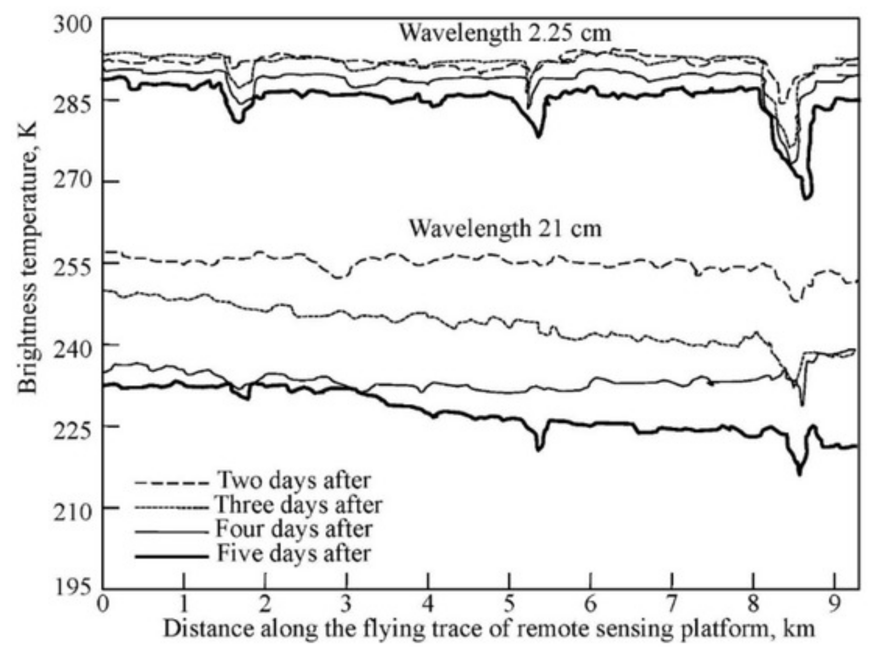
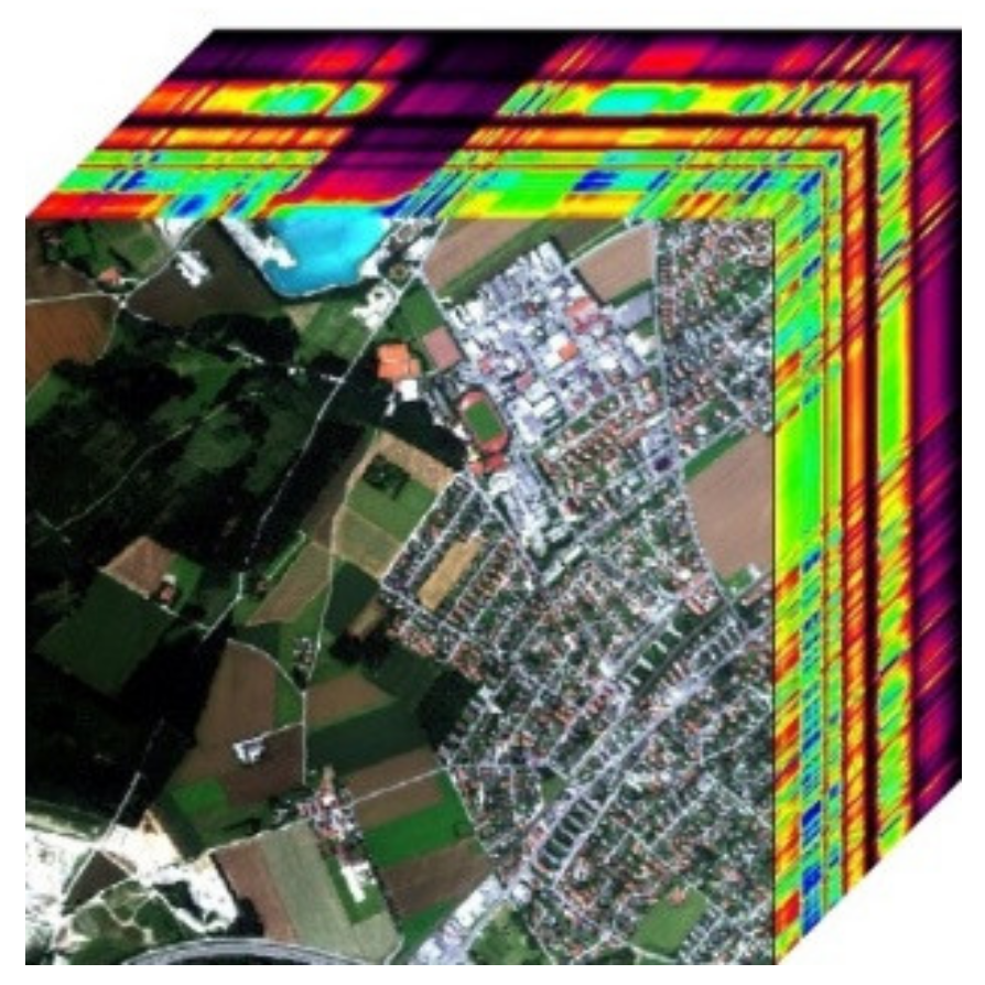
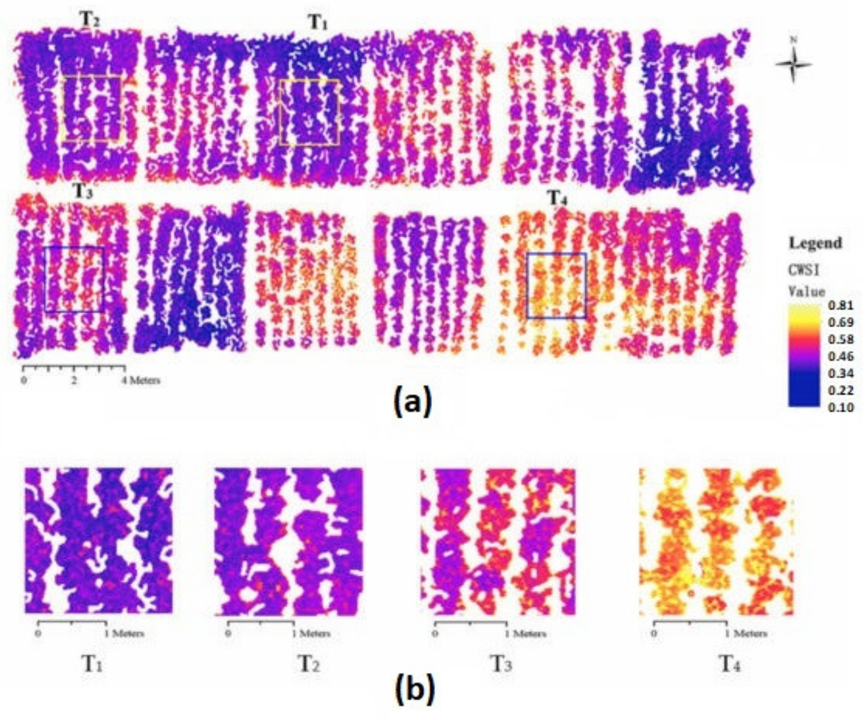
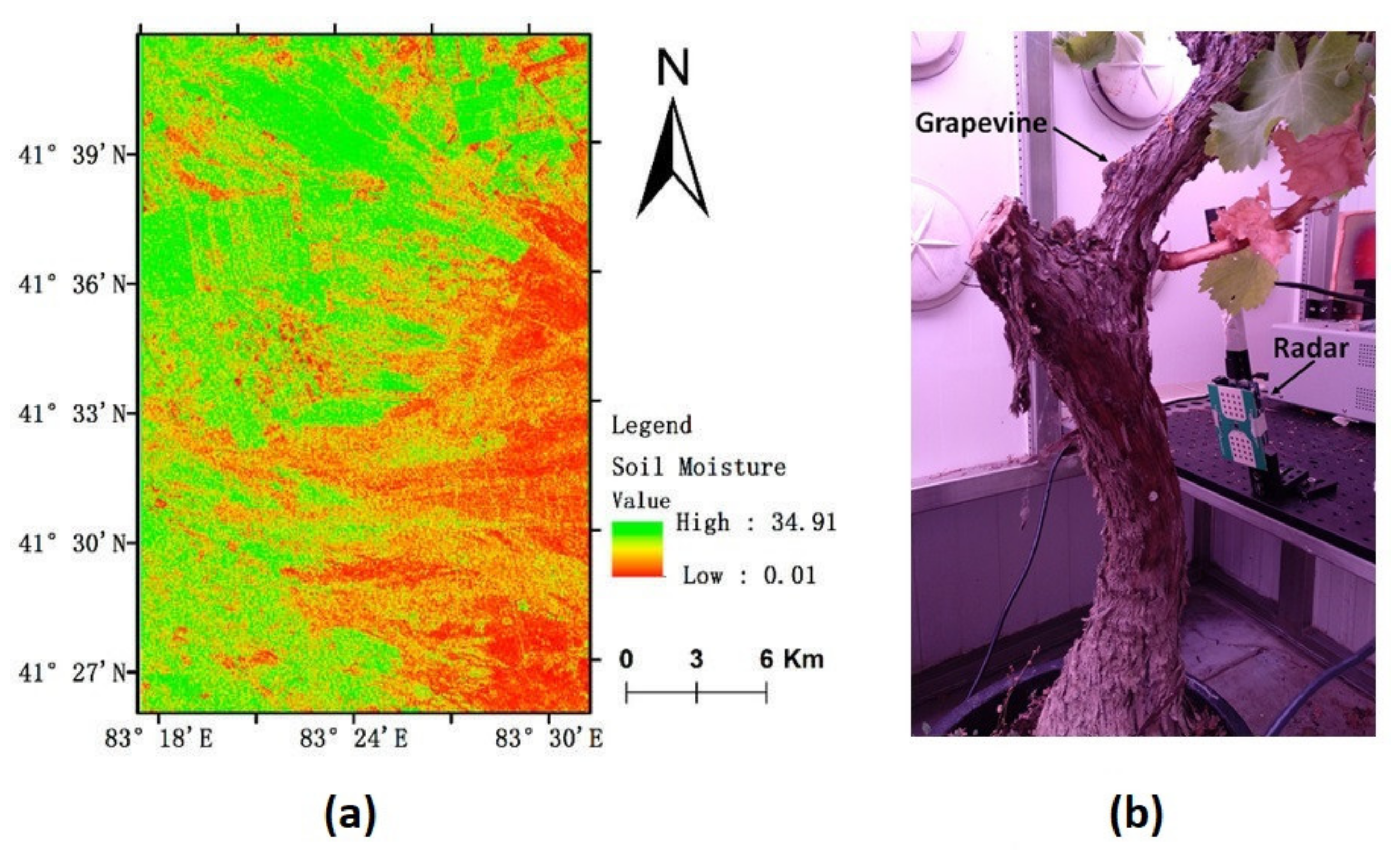
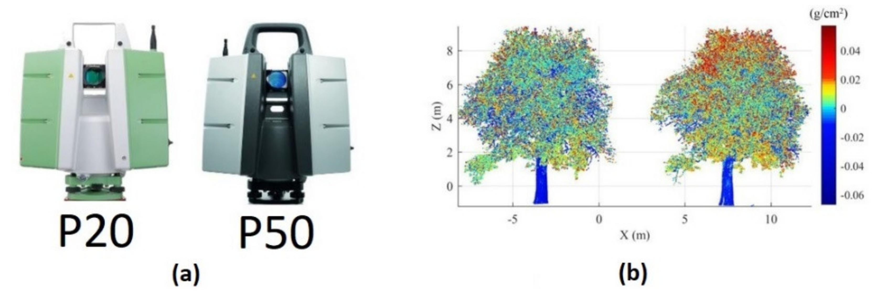
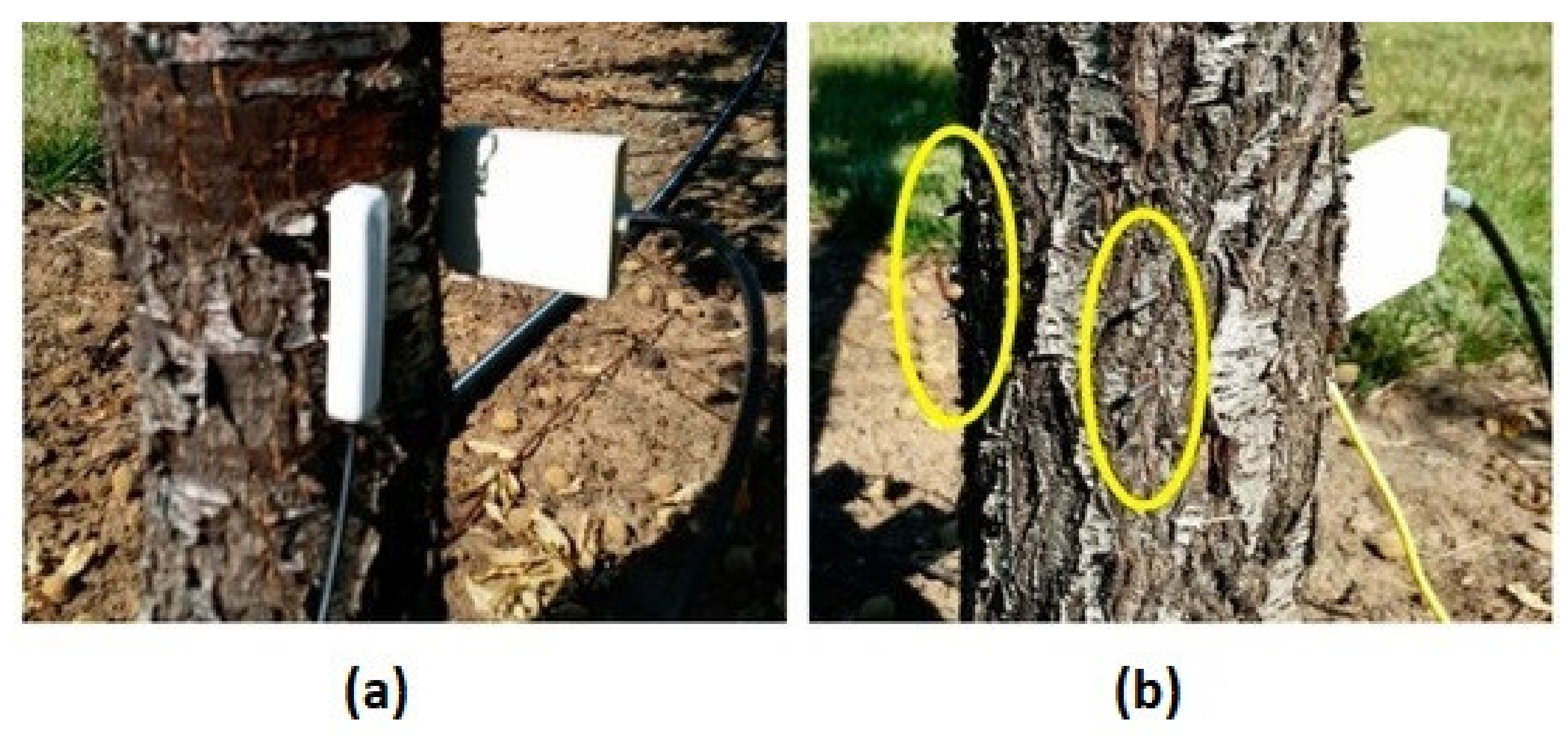
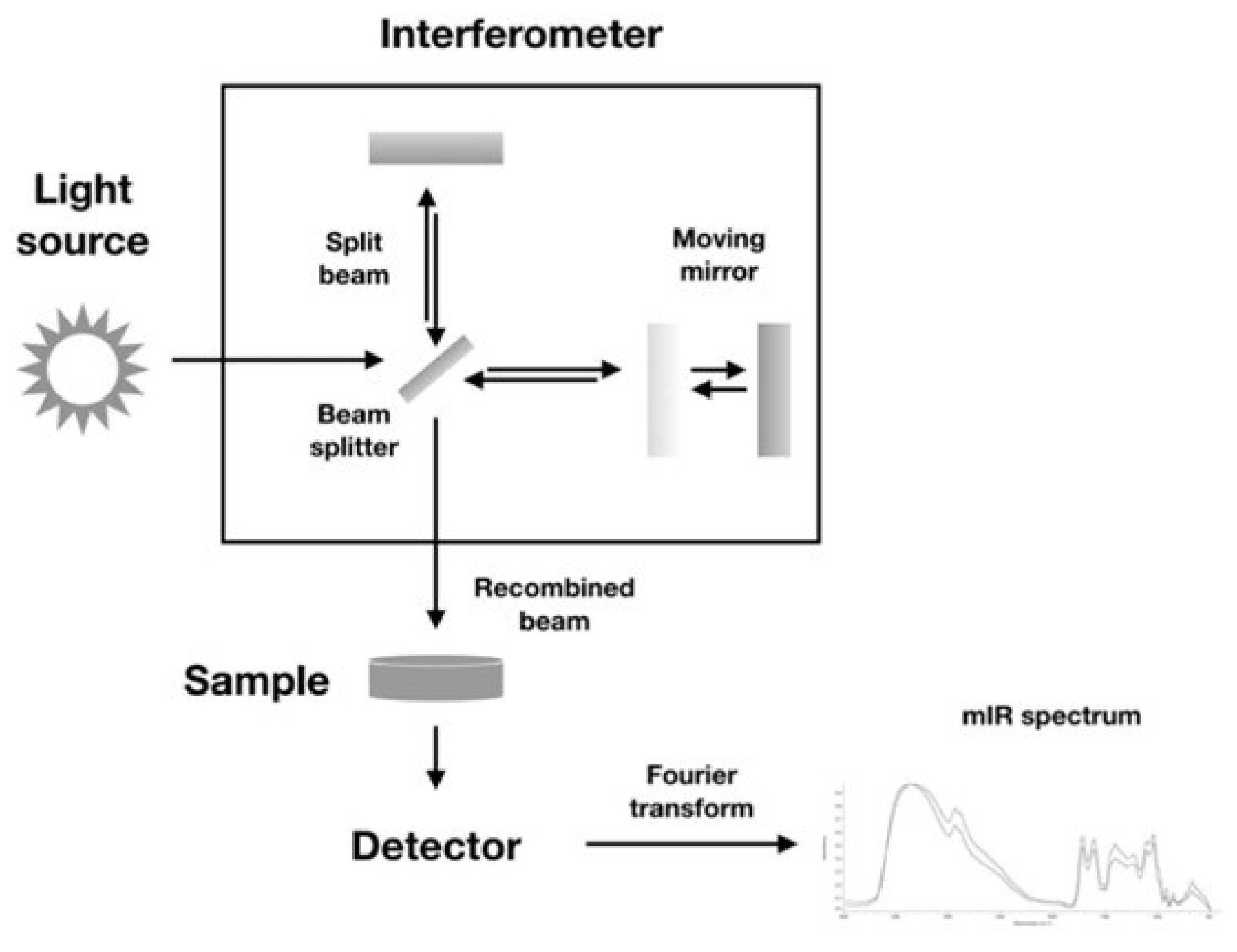
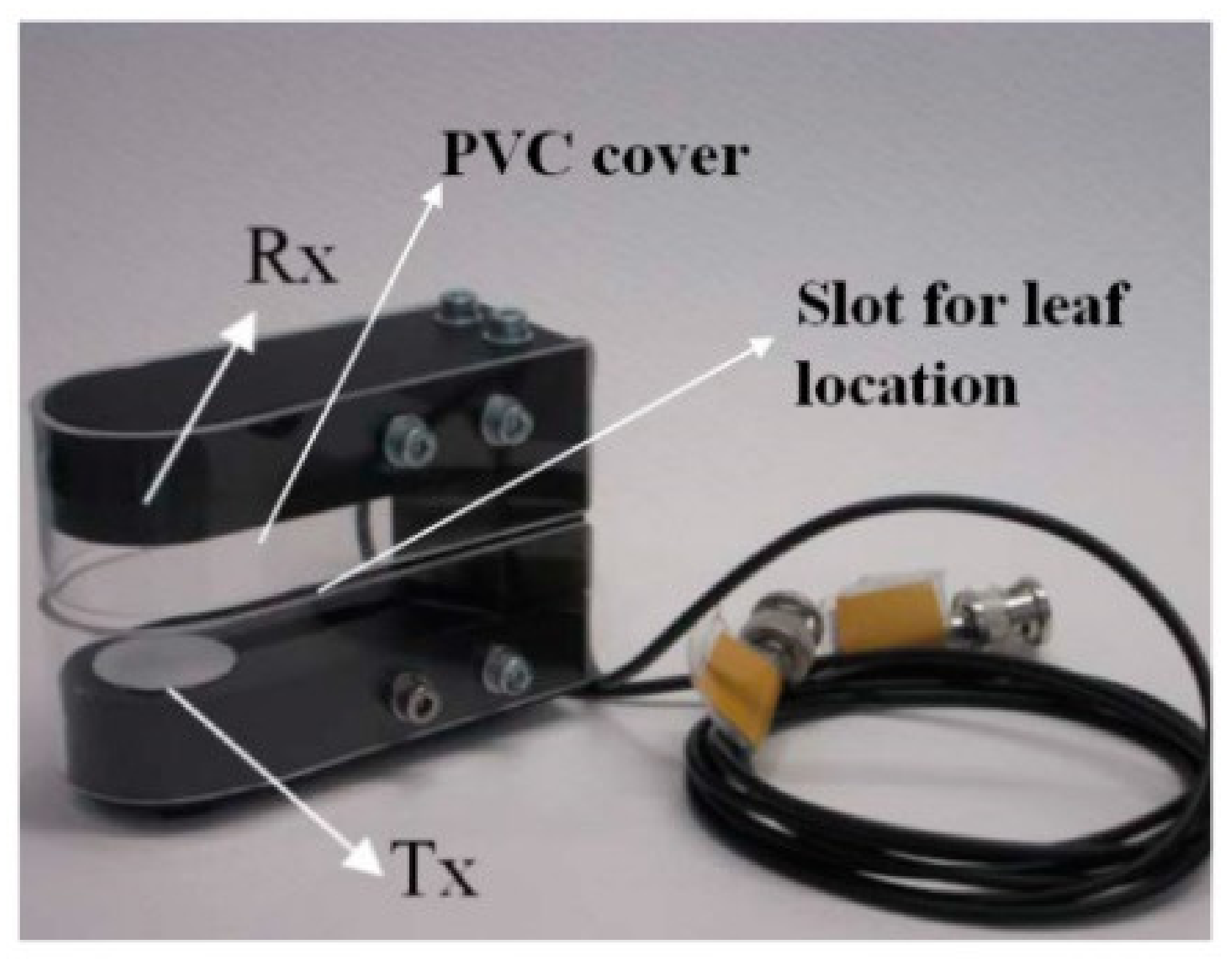
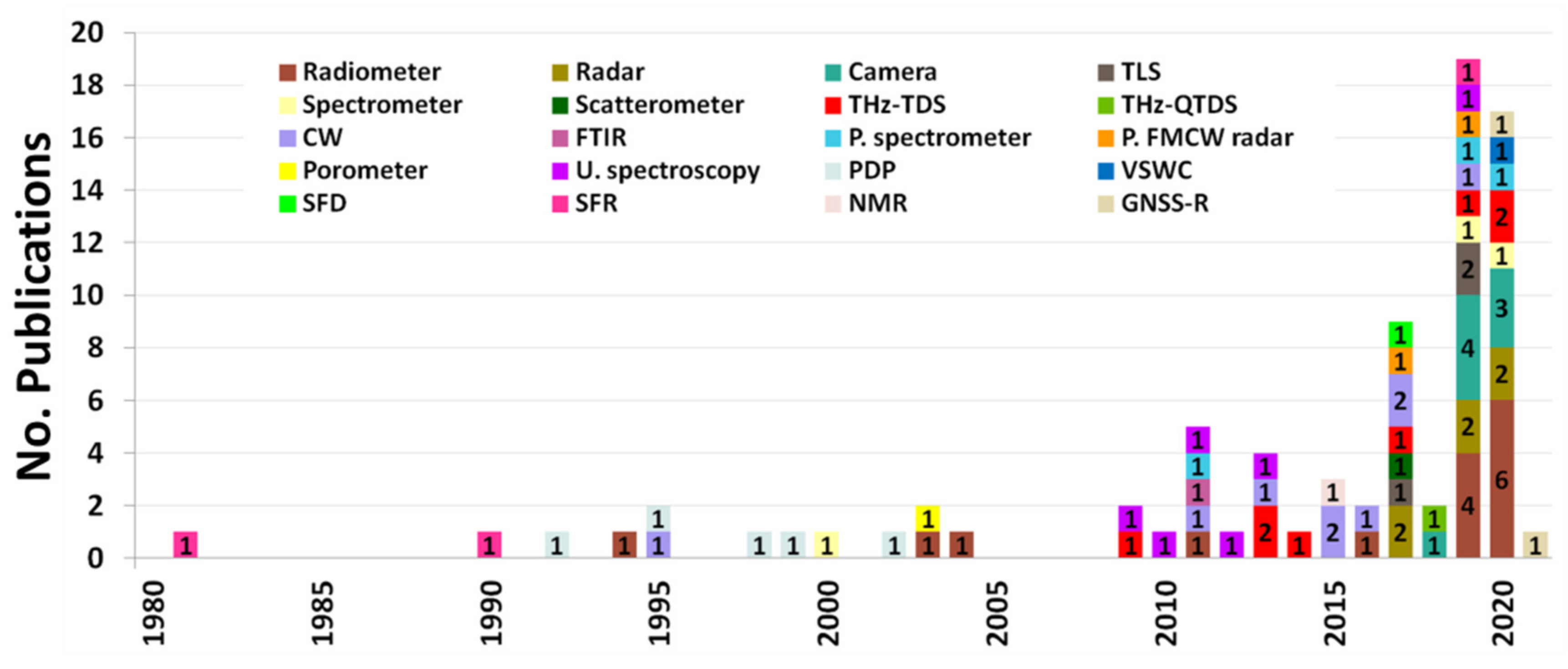
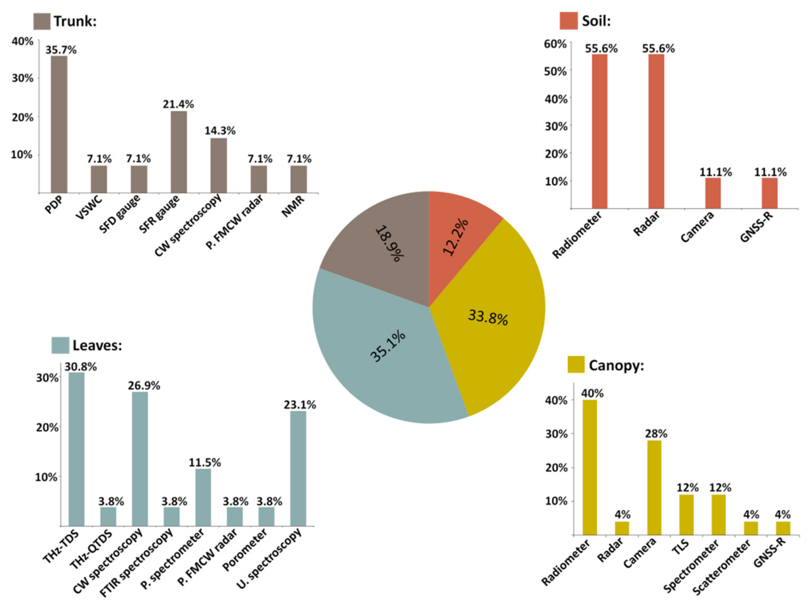
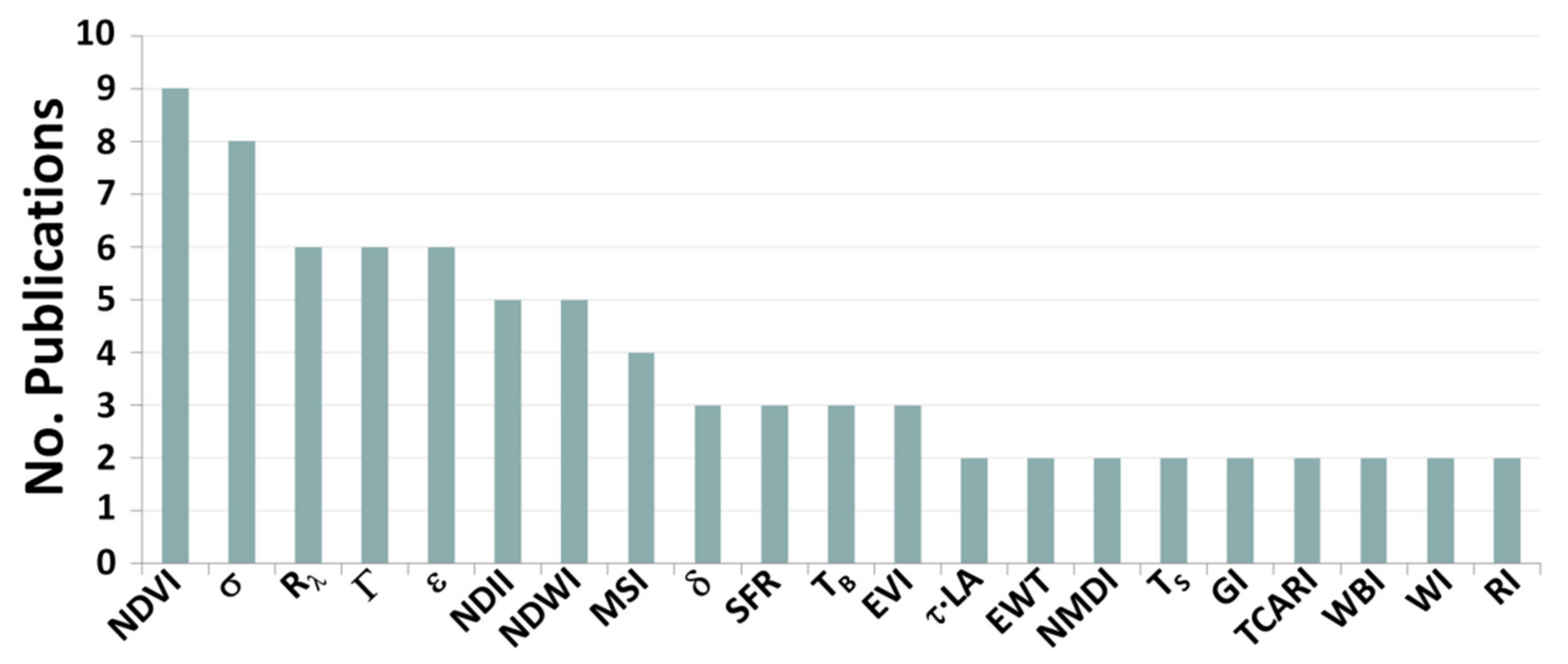
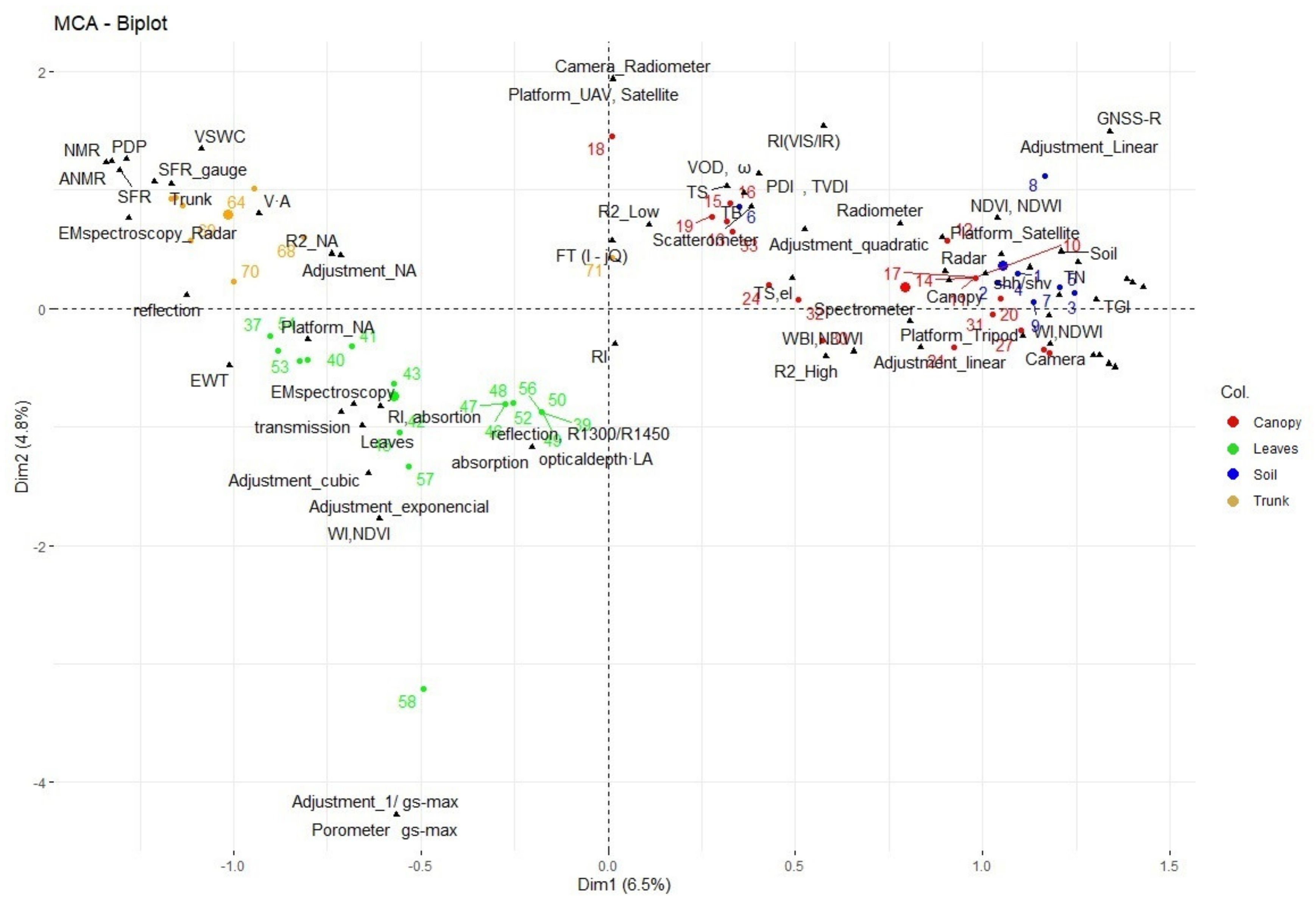
Table 1.
Main characteristics of the different electromagnetic spectroscopies used in this review.
| Technology | Components | Type of Signal | Frequency |
|---|---|---|---|
| THz-TDS | FS laser + Photoconductive antennas | Pulsed | THz |
| THz-CW | CW laser + Photoconductive antennas | Continuous | THz |
| THz-QTDS | Multimode laser diode | Pulsed | THz |
| CW-VNA | VNA + VNA extenders | Continuous | GHz, THz |
| FTIR | Michelson interferometer | Continuous | IR |
CW = Continuous-wave, FS = Femtosecond, FTIR = Fourier transform infrared, IR = Infrared, QTDS = Quasi time domain spectroscopy, TDS = Time domain spectroscopy, VNA = Vector network analyzer.
Table 2.
Summary of the estimators used in soil techniques together with the operating frequency, type of adjustment, R2, estimation error, technology, target and sensor platform.
Table 2.
Summary of the estimators used in soil techniques together with the operating frequency, type of adjustment, R2, estimation error, technology, target and sensor platform.
| Ref. | Estimator | Frequency | Adjustm. | R2 | Error | Technology | Target | Platf. |
|---|---|---|---|---|---|---|---|---|
| [9] | TN | 1.4 GHz | Linear | 0.7 | SEE = 3% | Rad. | S | Aircrf. |
| [10] | σ | 5.4 GHz | Linear | 0.64 | RMSE = 0.03 m3 ·m−3 | Radar | S | Sat. |
| [11] | TB, σ | 1.4 GHz | Linear | 0.794 | RMSE = 0.072 m3 ·m−3 | Radar, Rad. | S | Aircrf. |
| [12] | σ | 5.4 GHz | Linear | 0.676 | RMSE = 0.065 m3 ·m−3 | Radar | S | Sat. |
| [13] | σ, VWC | 5.4 GHz | Linear | 0.76 | RMSE = 2.04% | Radar, Rad. | S | Sat. |
| [14] | PDI, TVDI | NA | No fitting | NA | RMSE = 1.46% | Rad. | S | Sat. |
| [15] | σ, NDVI | 5.4 GHz | Linear | 0.806 | RMSE = 0.043 m3 ·m−3 | Radar, Rad. | S | Sat. |
| [16] | Rλ | 1.17, 1.57 GHz | Linear | 0.98 | SEE = 0.016 m3 ·m−3 | GNSS-R | S | Aircrf. |
| [17] | TGI | NA | Linear | 0.1024 | NA | Camera | S | UAV |
Aircrf. = Aircraft, GNSS-R = Global navigation satellite system-reflectometry, NDVI = Normalized difference vegetation index, PDI = Perpendicular drought index, Rad. = Radiometer, S = Soil, Sat. = Satellite, σ = backscattering coefficients, TB = brightness temperature, TGI = Triangular greenness index, TN = Normalized brightness temperature, TVDI = Temperature vegetation dryness index, UAV = Unmanned aerial vehicle, VWC = Vegetation water content.
Table 3.
Summary of the estimators used in canopy techniques together with the operating frequency, type of adjustment, R2, estimation error, technology, target and sensor platform.
Table 3.
Summary of the estimators used in canopy techniques together with the operating frequency, type of adjustment, R2, estimation error, technology, target and sensor platform.
| Ref. | Estimator | Frequency | Adjustm. | R2 | Error | Technology | Target | Platf. |
|---|---|---|---|---|---|---|---|---|
| [18] | TB, NDII | 10.7, 18.7, 37 GHz | Linear | 0.82 | RMSE = 0.96 Kg·m−2 | Rad. | C | Sat. |
| [19] | MR | 6.6, 37 GHz | Linear | 0.85 | RMSE = 10.91 s·m–1 | Rad. | C | Sat. |
| [20] | NDVI, NDWI | NA | Quadratic | 0.85 | RMSE = 0.171 Kg·m−2 | Rad. | C | Sat. |
| [21] | TB | 1.43, 13.3, 37.5 GHz | NA | NA | NA | Rad. | C | Aircrf. |
| [22] | nddVWC | 6.9, 10.7. 18.7 GHz | Linear | 0.6724 | NA | Rad. | C | Sat. |
| [23] | VOD, ω | 1.4, 6.9. 10.7 GHz | NA | NA | NA | Rad. | C | Sat. |
| [24] | Rλ | VIS/IR | No fitting | NA | RMSE = 0.41 m2·m−2 | Rad. | C | Sat. |
| [25] | NDWI | NA | Linear | 0.85 | RMSE = 0.94 Kg·m−2 | Rad. | C | Sat. |
| [26] | Rλ | VIS/IR | NA | NA | NA | Camera, Rad. | C | UAV, Sat. |
| [27] | TS | NA | NA | NA | NA | Rad. | C | Sat. |
| [28] | σ hh/σ hv | 1.26 GHz | Linear | 0.81 | RMSE = 0.12 Kg·m−2 | Radar | C | Aircrf. |
| [29] | C/N0 | 1.57 GHz | Linear | 0.92 | 0.49 dB | GNSS-R | C | Ground |
| [30] | Rλ | VIS/IR | Linear | 0.99 | NA | Camera | C | UAV |
| [31] | VSWI = VI/Tc | VIS/IR | Linear | 0.998 | NA | Camera | C | UAV |
| [32] | CWSIsi | NA | Linear | 0.66 | NA | Camera | C | UAV |
| [33] | TS, ελ | 25–38.46 THz | NA | NA | NA | Camera | C | Tripod |
| [34] | DANS | NA | Linear | 0.77 | NA | Camera | C | UAV |
| [35] | WSI, CWSI | NA | Linear | 0.94 | NA | Camera | C | UAV |
| [36] | σ | 1550 nm | Linear | 0.85 | RMSE = 0.0016 g·cm−2 | TLS | C | Tripod |
| [37] | NDII | NA | Linear | 0.93 | RMSE = 0.00065 g·cm−2 | TLS | C | Tripod |
| [38] | NDII | NA | Linear | 0.94 | RE = 6.3% | TLS | C | Tripod |
| [39] | WBI, NDWI | NA | Linear | 0.8464 | NA | P. spectm. | C | |
| [40] | WI, NDWI | NA | Linear | 0.88 | NA | Spectm. | C | Aircrf. |
| [41] | VIs from Rλ | VIS/IR | NA | ~1 | NA | Spectm. | C | Aircrf. |
| [42] | σ | 13.6 GHz | NA | NA | NA | Scatterometer | C | Sat. |
Aircrf. = Aircraft, C = Canopy, C/N0 = carrier-to-noise ratio, CWSIsi = Simplified crop water stress index, DANS = Degrees above non-stress, ελ = Emissivity, GNSS-R = Global navigation satellite system-reflectometry, IR = Infrared, MR = Moisture ratio, nddVWC = Normalized diurnal difference vegetation water content, NDII = Normalized difference infrared index, NDVI = Normalized difference vegetation index, NDWI = Normalized difference water index, P. = Portable, Rad. = Radiometer, Rλ = Spectral reflectance, Sat. = Satellite, Spectm. = Spectrometer, σ = Backscattering coefficients, TB = Brightness temperature, Tc = Canopy temperature, TLS = Terrestrial laser scanning, TS = Land surface temperature, UAV = Unmanned aerial vehicle, VI = Vegetation index, VIS = Visible, VOD = Vegetation optical depth, VSWI = Vegetation water supply index, ω = Single scattering albedo, WBI = Water band index, WI = Water index, WSI = Water stress integral.
Table 4.
Summary of the estimators used in leave techniques together with the operating frequency, type of adjustment, R2, estimation error, technology, target and sensor platform.
Table 4.
Summary of the estimators used in leave techniques together with the operating frequency, type of adjustment, R2, estimation error, technology, target and sensor platform.
| Ref. | Estimator | Frequency | Adjustm. | R2 | Error | Technology | Target | Platf. |
|---|---|---|---|---|---|---|---|---|
| [43] | T | THz | No fitting | NA | RMSE = 2% | THz-TDS | L (D) | NA |
| [44] | RI, δ | 0.3–1.8 THz | NA | NA | NA | THz-TDS | L (D) | NA |
| [45] | T | 0.1–2 THz | NA | NA | NA | THz-TDS | L (D) | NA |
| [46] | Г | 10 GHz | NA | NA | NA | CW spects. | L (D) | NA |
| [47] | T | 0.75–1.1 THz | No fitting | NA | RE = 1.2% | CW spects. | L (D) | NA |
| [48] | Г, R1300/R1450 | 1730 MHz | Linear | 0.98 | SEE = 0.00394 | CW spects., P. spectm. | L (D) | NA |
| [49] | Rλ | 3–15 μm | NA | NA | NA | FTIR spects. | L (D) | NA |
| [50] | Rλ | 350–2500 nm | No fitting | NA | RE < 10% | P. spectm. | L (D) | NA |
| [51] | T | 0.3–1.2 MHz | Cubic | 0.99 | NA | U. spects. | L (D) | NA |
| [52] | T | 0.3–1.3 MHz | Unknown | 0.99 | NA | U. spects. | L (D) | NA |
| [53] | T | 0.2–1.3 MHz | No fitting | NA | NA | U. spects. | L (D) | NA |
| [54] | T | 0.3–1.2 MHz | Cubic | 0.99 | NA | U. spects. | L (D) | NA |
| [55] | T, S | 0.3–1.2 MHz | Linear | 0.995 | NA | CW spects., U. spects. | L (D) | NA |
| [56] | T | 0.15–1.6 MHz | Linear | 0.8464 | RMSE = 0.04 | U. spects. | L (D) | NA |
| [57] | RI, δ | 0.6–1.8 THz | Linear | 0.8377 | RMSE = 0.0526% | THz-TDS | L (ND) | NA |
| [58] | τ·LA | 2.55 THz | Linear | 0.99 | NA | THz-TDS | L (ND) | NA |
| [59] | τ·LA | 2.55 THz | Linear | 0.95 | NA | THz-TDS | L (ND) | NA |
| [60] | T | 0.1–2 THz | NA | NA | NA | THz-TDS | L (ND) | NA |
| [62] | T | 150–300 GHz | Linear | 0.9604 | NA | THz-TDS | C, L (ND) | NA |
| [63] | EWT | 100–200 GHz | NA | NA | NA | THz-QTDS | L (ND) | NA |
| [64] | Г | 2.1–4.1 GHz | NA | NA | NA | CW spects. | L (ND) | NA |
| [65] | T | 0.1–1.1 THz | No fitting | NA | SD(0.4 THz) > 0.3 | CW spects. | L (ND) | NA |
| [66] | δ | 35 GHz | Linear | 0.83 | RMSE = 0.17 g | CW spects. | L (ND) | NA |
| [67] | WI, NDVI | NA | Exp. | 0.69 | NA | P. spectm. | L (ND) | NA |
| [68] | Г | 25.86–37.51 GHz | Quadratic | 0.99 | RMSE = 0.27% | P. FMCW Radar | F (ND) | NA |
| [69] | gs-max | NA | 1/gs-max | 0.98 | NA | Porometer | L (ND) | NA |
C = Canopy, CW = Continuous-wave, Г = Reflection coefficient, δ = Absorption coefficient, D = Destructive, EWT = Equivalent water thickness, F = Fruit, FMCW = Frequency-modulated continuous-wave, FTIR = Fourier transform infrared, gs-max = Maximal stomatal conductance, L = Leaves, LA = Leaf surface area, ND = Non-destructive, NDVI = Normalized difference vegetation index, P. = Portable, QTDS = Quasi time domain spectroscopy, RI = Refractive index, S = Existing area, Spectm. = Spectrometer, Spects. = Spectroscopy, T = Transmission coefficient, TDS = Time domain spectroscopy, τ = Leaf optical depth, U. = Ultrasonic, WI = Water index.
Table 5.
Summary of the estimators used in trunk techniques together with the operating frequency, type of adjustment, R2, estimation error, technology, target and sensor platform.
Table 5.
Summary of the estimators used in trunk techniques together with the operating frequency, type of adjustment, R2, estimation error, technology, target and sensor platform.
| Ref. | Estimator | Frequency | Adjustm. | R2 | Error | Technology | Target | Platf. |
|---|---|---|---|---|---|---|---|---|
| [71] | ε | 0.5 GHz | NA | NA | NA | PDP | T (I) | NA |
| [72] | ε | 1.25 GHz | NA | NA | NA | PDP | T (I) | NA |
| [73] | ε | 0.45, 1.2 GHz. 5 GHz | NA | NA | NA | PDP | T (I) | NA |
| [74] | ε | 1.25 GHz | NA | NA | NA | PDP | T (I) | NA |
| [75] | ε | 1–10 GHz | NA | NA | NA | PDP | T (NI) | NA |
| [76] | ε | 70, 78 MHz, 3.5, 4 GHz | Unknown | 0.29 | NA | VSWC | T (I) | NA |
| [78] | SFR | NA | NA | NA | NA | SFR gauge | T (NI) | NA |
| [79] | SFR | NA | No fitting | NA | RMSE = 69 g·plant–1·d–1 | SFR gauge | T (NI) | NA |
| [80] | SFR | NA | NA | NA | NA | SFR gauge | T (NI) | NA |
| [81] | V·A | NA | NA | 0.94 | NA | SFD gauge | T (I) | NA |
| [82] | Г | 0.14–0.22 THz | NA | NA | NA | CW spects. | T (NI) | NA |
| [83] | Г | 0.14–0.22 THz | NA | NA | NA | CW spects., Radar | T (NI) | NA |
| [84] | FT(I–jQ) | 21.4–24.8 GHz | Quadratic | 0.995 | NA | P. FMCW Radar | T (NI) | NA |
| [85] | ANMR | NA | NA | NA | NA | NMR | T (NI) | NA |
A = Stem area, ANMR = Amplitude of the NMR signal, CW = Continuous-wave, Г = Reflection coefficient, ε = Dielectric constant, FMCW = Frequency-modulated continuous-wave, FT = Fourier transform, I = Invasive, I and Q = Output signals of the radar’s IQ mixer, NI = Non-invasive, NMR = Nuclear magnetic resonance, P. = Portable, PDP = Portable dielectric probe, SFD = Sap-flux density, SFR = Sap-flow rate, Spects. = Spectroscopy, T = Trunk, V = Apparent heat pulse velocity, VSWC = Volumetric soil water content.
Publisher’s Note: MDPI stays neutral with regard to jurisdictional claims in published maps and institutional affiliations. |
© 2021 by the authors. Licensee MDPI, Basel, Switzerland. This article is an open access article distributed under the terms and conditions of the Creative Commons Attribution (CC BY) license (https://creativecommons.org/licenses/by/4.0/).
Share and Cite
MDPI and ACS Style
Quemada, C.; Pérez-Escudero, J.M.; Gonzalo, R.; Ederra, I.; Santesteban, L.G.; Torres, N.; Iriarte, J.C. Remote Sensing for Plant Water Content Monitoring: A Review. Remote Sens. 2021, 13, 2088. https://doi.org/10.3390/rs13112088
AMA Style
Quemada C, Pérez-Escudero JM, Gonzalo R, Ederra I, Santesteban LG, Torres N, Iriarte JC. Remote Sensing for Plant Water Content Monitoring: A Review. Remote Sensing. 2021; 13(11):2088. https://doi.org/10.3390/rs13112088
Chicago/Turabian StyleQuemada, Carlos, José M. Pérez-Escudero, Ramón Gonzalo, Iñigo Ederra, Luis G. Santesteban, Nazareth Torres, and Juan Carlos Iriarte. 2021. "Remote Sensing for Plant Water Content Monitoring: A Review" Remote Sensing 13, no. 11: 2088. https://doi.org/10.3390/rs13112088
Note that from the first issue of 2016, this journal uses article numbers instead of page numbers. See further details here.