
A Survey of Rain Fade Models for Earth–Space Telecommunication Links—Taxonomy, Methods, and Comparative Study


1
Department of Information and Communication Engineering, Chosun University, Gwangju 61452, Korea
2
Department of Electronics and Telecommunication Engineering, International Islamic University Chittagong, Chittagong 4318, Bangladesh
3
Department of Electronics and Communication Engineering, Adama Science and Technology University, Adama 1888, Ethiopia
*
Author to whom correspondence should be addressed.
Remote Sens. 2021, 13(10), 1965; https://doi.org/10.3390/rs13101965
Submission received: 2 April 2021
/
Revised: 12 May 2021
/
Accepted: 13 May 2021
/
Published: 18 May 2021
(This article belongs to the Special Issue Advanced Satellite-Terrestrial Networks)
Abstract
:Satellite communication is a promising transmission technique to implement 5G and beyond networks. Attenuation due to rain begins at a frequency of 10 GHz in temperate regions. However, some research indicates that such attenuation effects start from 5–7 GHz, especially in tropical regions. Therefore, modeling rain attenuation is significant for propagating electromagnetic waves to achieve the required quality of service. In this survey, different slant link rain attenuation prediction models have been examined, classified, and analyzed, and various features like improvements, drawbacks, and particular aspects of these models have been tabulated. This survey provides various techniques for obtaining input data sets, including rain height, efficient trajectory length measurement techniques, and rainfall rate conversion procedures. No survey of the Earth–space link models for rain attenuation is available to the best of our knowledge. In this study, 23 rain attenuation models have been investigated. For easy readability and conciseness, the details of each model have not been included. The comparative analysis will assist in propagation modeling and planning the link budget of slant links.
1. Introduction
Satellite communication is playing major role in the back-haul data network. In addition, satellite communication links can be used to enhance the existing telecommunication infrastructure in 5G and beyond networks [1,2,3], and satellite communication also has enormous applications for unmanned aerial vehicles (UAVs) and the Internet of Things (IoT) [4]. Because of radio congestion and broader bandwidth requirements, satellites switch to higher-frequency (33–75 GHz and 75–110 GHz) bands. However, atmospheric disturbances wreak havoc on these frequencies, causing attenuation, scintillation, and depolarization, lowering service efficiency [5]. Rain is one of the significant factors that creates attenuation on the propagation of electromagnetic waves. This effect has directed the interest of researchers in reducing the effect of rain on radio waves by controlling the transmitted power. Thus, multiple studies have been conducted on this globally. The research on rain attenuation is used to predict rain attenuation in various geographical areas over a wide range of frequency bands, especially for frequency bands over 10 GHz, and determine a suitable model that can predict attenuation. To develop such a model, the factors that impact attenuation first need to be determined. Some of the factors are related to the infrastructure setup (latitude, longitude, antenna size, antenna height, elevation angle, operating frequency) and some of them are related to the rain events such as wind flow, humidity, wind direction, and temperature.
It may be possible to evaluate the attenuation of atmospheric elements such as wind flow and the effect of the direction of wind flow on propagated signal attenuation separately, but it is conventional to consider attenuation due to other factors such as temperature, wind flow, and wind direction, along with rain attenuation. Even though rain attenuation issues were noticed in the middle of the last century, the problem has not yet been efficiently addressed. Besides the necessity to transfer a massive volume of data due to the fourth industrialization, the lower frequency bands are getting exhausted. This has led researchers to develop rain attenuation models that can work with higher frequency bands such as Q/V, W, and E-bands. For example, the application of a rain attenuation model for slant link, where the operating frequency is at 75 GHz, was assessed in [6,7]. Several models of rain attenuation have been proposed in the literature, and scientists are aiming to refine existing models for local climate conditions [8,9,10,11,12,13].
Precise rain attenuation determinations are critical for preparing the link budget, maintaining communication efficiency, and the architecture of the system. In addition, following probable rain attenuation determined by the rain attenuation model, the over- or underestimation of the power of the transmitter can be avoided. Radio-frequency engineers must comply with the permissible power transmission specifications in compliance with spectrum management rules for each frequency band. If the engineers do not follow such power regulations, the transmitted signal power may interfere with another frequency band, e.g., neighbor channel, which may disturb the neighboring telecommunication equipment. Thus, by deploying a rain attenuation model in Earth–space telecommunication, such disturbance can also be avoided. In the literature, there is currently a lack of survey papers addressing the issues and algorithms of slant link fade prediction models, which inspired us to write this survey paper. In Table 1, some of the existing survey papers are presented, which are not adequate for covering the slant link fade prediction models.
Previously, we surveyed the recent literature in relation to terrestrial link rain attenuation models [17], which is also clearly different compared to the current study, as our previous terrestrial link survey was on Earth-to-Earth links only. Rain affects the propagation of electromagnetic waves both on the Earth–space and terrestrial links. The rain attenuation model for the Earth–space link is used to manage the rain attenuation on the Earth–satellite telecommunication link management. In comparison, the rain attenuation model is used to manage the rain attenuation on the Earth-to-Earth links. Thus, these two types of link are different although they have a resemblance. Even ITU-R proposed a separate model for rain attenuation for the Earth–space (ITU-R P.618 series) and terrestrial links (ITU-R P.530 series). Further differences between the Earth–space and terrestrial links are given in Table 2.
This paper presents findings such as classification of well-known rain attenuation models, supporting the frequency range, applicability to Earth–satellite links, and improvements or limitations of the models.
This study extensively investigates the well-known and essential features of up-to-date models, drawbacks, and unique features. We have also qualitatively compared the slant link rain attenuation models. The significant contributions of this study are as follows:
- To the best of our knowledge, slant link rain fade models have not been classified broadly. In this work, we have prepared a taxonomy of the rain fade models for Earth–space links.
- A brief overview of each of the models selected is presented. In addition, we have provided algorithms of different models.
- Quantitative and qualitative characteristics of different models are organized in tables to review comparative studies.
- We noticed that each model was improved inherently and criticized the prototype by finding the inconveniences, and the specific characteristics are listed.
- Finally, the open research issues are summarized.
The remainder of this paper is organized as follows: Section 2 describes related parameters of Earth–space rain attenuation models. In Section 3, a taxonomy of existing models is presented. In Section 4, core insights of the models, algorithms, advantages, and limitations are discussed. In Section 5, comparative studies among the models are presented. In Section 6, open issues and research challenges are summarized and discussed. Finally, concluding remarks are presented in Section 7.
2. Background Study
The most significant impacts on the propagation of slant microwave and millimetric wave links are hydrometeors such as thunder, hail, rain, ice, and snow. Among these parameters, rainfall attenuation is the most important phenomenon. The raindrops act as dielectric particle loss, which causes dispersion and depolarization.
2.1. Rain Attenuation Parameters
Developing a rain fade model involves mathematical analysis of rain attenuation phenomena by reasoning and cause-based interaction. A broad range of variables that can impact the rain attenuation is given in [15,18,19,20,21,22,23,24,25,26]. The parameters that affect the rain attenuation are rainfall rate, frequency, path length in the precipitation, temperature, humidity, wind velocity, wind direction, visibility, polarization, raindrop radius, raindrop size, latitude, elevation angle, station height, raindrop cross-section, depolarization loss, and refractive index of the air.
2.2. Earth–Space Link Budget
For rain attenuation studies and measurement, link budgeting is concerned with the losses and gains at the receiver antenna. The link budget does not differ much from terrestrial links except that free space loss (FSL) is much higher due to the considerable distance between the transponder and the Earth station [23,24,25,27].
where is the transmitter power. This is the microwave carrier output power, expressed in in Equation (1); L is losses due to the presence of atmospheric gases, vegetation, buildings, clouds, and fog; is the transmitter antenna gain, is the receiver antenna gain, FSL is the free space path loss in dB, and is the received signal level in dBm. Compared to terrestrial links discussed in [17], FSL is higher, e.g., above 200 dB in Ka/Q bands [25]. The performance of a communication system is estimated based on the achievable signal-to-noise ratio (SNR) at the receiver. The term SNR (in dB) refers to the estimation of signal strength as a function of signal degradation and background noise. This SNR can be expressed as:
where is system loss at the receiver and transmitter; is free-space wavelength (m), which is determined from the frequency as ; and are transmitting and receiving antenna gains, respectively; k is the Boltzmann constant J/K; B is the bandwidth in (Hz); l is the link distance (m); and T is the noise temperature (K) of the system, which is assumed to be 290 K.
Equation (2) can equivalently be computed in unit decibels (dBm) as
where is determined from the link profile given parameters. In real-world radio links, for the communications system to acquire the least tolerable quality of service (usually termed as minimum SNR), the received power level often needs to be better than the threshold level. When the received signal magnitude is below the threshold value, a network outage will occur. As a result, the radio link performance evaluation is done by comparing the percentage of outage time with the total time duration. This design allowance for received power is termed as the link margin and defined as the difference between the design value of received power and the minimum threshold value of received power [25,26]:
where LM denotes the link margin measured in . LM, which is used to account for fading effects, is sometimes referred to as fade margin.
Clear Air SNR calculation: The received signal for clear-sky conditions is determined using Equation (1) and the SNR of this link in a clear-sky environment can be determined using (6).
Rainy time SNR calculation: Here the received signal is additionally degraded by the total rain attenuation amount. Thus, SNR at a rainy time is calculated as [23]:
where is the attenuation induced by rain. If the SNR at a rainfall rate of exceedance of is required, it can be calculated by replacing by total rain attenuation at a rainfall rate of exceedance of .
2.3. Rain Attenuation Anomalies: Breakpoint
At a breakpoint, the monotonous behavior of the time exceedance of rain changes abruptly in tropical regions. The breakpoint is more visible if the integration is considered over a smaller time duration; however, according to [29], a 1 min rainfall rate integration is the optimum time to clarify the rain structure to avoid noise. The main reason for modifying the model is considering the non-monotonous behavior of rain attenuation in tropical areas. It is found that there is a breakpoint of rainfall rate attenuation while moving from the temperate region to the tropical area, where the integration time is comparatively short. For such existing breakpoints, many of the temperate region models do not fit well in the tropical regions, and based on this, breakpoint idea-based models have been proposed in [30,31].
2.4. Slant Path in Rain Cell
The path length that remains in the rain cell structure suffers rain attenuation. There may be some other meteorological effects on the extended portion of the slant link, but there exists no rain attenuation effect. As a result, the slant path length that falls within the rain cell must be determined. However, since the length exists in the space, it is impossible to determine precisely, rather than considering the estimated length. The rain height estimation helps to estimate the slant path length in the precipitation.
2.4.1. Rain Height
In many rain attenuation models [32,33,34], the rain height is used to determine the slant link length. However, the rain height is not uniform in every location of the world, so it is crucial to estimate the rain height in a specific geographical area. For a low rainfall rate, the minimum rain height is about 4 km, although there are variations in different models. However, some of the models estimate rain heights with elevation angles and rainfall rate as well. Table 3 lists most of the estimation techniques for rain height determination.
2.4.2. Effective Slant Path
The effective path length is the length of a conceptual path derived from radio data by dividing overall attenuation by actual attenuation exceeded over the same percentage of the time. The total attenuation is determined as [35]:
where is the total attenuation due to rain, and specific attenuation of the link is , then the “effective path length” is defined by . Table 4 shows a list of additional techniques to determine ‘effective path length.
2.5. Rainfall Rate Conversion
The rainfall rate is the main parameter to determine the rain attenuation. The rainfall rate is measured in mm per time unit. Depending on the sensor device used to record the rainfall rate, the integration time unit may be 10 s, 20 s, to 1 min, 5 min, or even 1 h. The rain attenuation model may need to convert the rainfall rate over different integration times. The International Telecommunication Union-Radiocommunication sector (ITU-R) P.618 [45] recommends applying a 1 min integration time. If local rain data are available in other integration times, the rainfall rate needs to be converted. Table 5 lists most of the rainfall rate conversion techniques, as per the literature. Instead of a mathematical conversion procedure, the rainfall rate “contour map” can be used to obtain the rainfall rate [40,46,47,48].
Even if the rainfall rate is not readily available, or there are missing data in the collected records, there also exist synthetic techniques to generate rain attenuation time series. Mathematically, Equation (10) defines the rainfall rate in a typical rainfall rate acquisition system:
where is rainfall rate, is rainfall per tip (mm), N is number of tips, and T is the time gap between consecutive tips.
2.6. Rain Type
In total, two types of rain, known as stratiform and convective precipitation, exist. The convective rain is heavy; thus, the propagated radio waves attenuated by convective rain are heavily attenuated. Conversely, stratiform rain is comparatively light and comparatively less attenuated. Therefore considering the effects of different rain types can yield better-predicted attenuation. For example, the rain attenuation model in [62] considers stratiform and convective rainfall to predict rain attenuation. The convective type is heavy rain that corresponds to a high rainfall rate and stratiform rain corresponds to light rain and hence low rainfall rate. The structure of the rain cell is also incorporated with the rainfall rate, which is shown in Figure 1.
2.7. Rain Cell Size
2.8. Rainfall Rate Missing Data
2.8.1. Temporal Missing: Time Series (TS)
The rain attenuation prediction requires long-term local rainfall rate information. However, in all parts of the world, such rainfall rate datasets are not available. In addition, even though the rainfall rate or rain attenuation datasets are recorded for a specific experimental setup, some parts of the dataset might be missing. To address these issues, a rainfall rate or attenuation time series needs to be generated. Fortunately, there are techniques available such as the synthetic storm technique (SST) [63] and enhanced synthetic storm technique (ESST) [64], and 2-D SST [65]. Rain attenuation prediction models such as the global synthetic storm technique (GSST) model [66] and the ESST model [64] use such types of time series generation procedures. Through applying such a procedure, as stated earlier, the missing datasets of any local climate can be generated.
2.8.2. Temporal Missing: Generation by Synthetic Means
The synthetic way to generate the rainfall rate of a locality needs local statistical distribution of the point rainfall intensity that feeds to the model, known as the exponential cell (EXCELL) model [67]. This model offers two types of rain cell structure, called the monoaxial model and the biaxial model. In a monoaxial model, the cell is presumed to be circular, and in a biaxial model, the model is assumed to be elliptical, and the monoaxial or biaxial property is determined by the orientation of central moments of inertia. In the EXCELL model, a typical rain cell can be defined by the following parameters: cell area (A), cumulative rain (Q), average rainfall rate (), root mean square (RMS) of rainfall rate (), rain cell gravity center (), and the central moments of inertia (). These parameters can be estimated from the local peak rainfall rate () and rain cell radius () in the () plane through which the rainfall rate decreases at the rate of (note the exponential form). It is notable that the simple rain attenuation model (SAM) [32] and the LU model [68] inherently include distance as a negative exponential factor to determine the spatial rainfall rate. This hypothesis induces error if the rain cell area is smaller than 5 km2 and the rainfall rate is smaller than 5 mm/h (). To describe the rain cell model for the EXCELL model, the parameters that must be considered are as per Table 6:
A variant of the EXCELL model is the HYCELL model [69], where the rainfall rate is considered a result of an exponentially decreasing rainfall rate (), normally distributed (Gaussian process) rainfall rate, and as a finite linear combination of these two types of rainfall distribution. These two approaches of determining the rainfall rate are applicable separately depending on a specified rainfall rate () that acts as boundary value defining the application of the Gaussian process and the exponential rate to be used. Thus, if the rainfall rate satisfies , the rainfall rate distribution is generated through the exponential parameter, and if it is greater than the Gaussian process parameter is applied. The EXCELL and HYCELL models contribute to developing a single rain cell that may not cover a long link. Consequently, an extended version of the EXCELL model covering a long link was proposed in the literature, which is known as the MultiEXCELL model (a kind of propagation-oriented precipitation model based on a cellular rain formulation) [70]. In the MultiEXCELL model, instead of the biaxial elliptical approach, the monoaxial approach was considered. The minimum rain cell area was set 4 km2 and the other distinct parameters were similar to the EXCELL model (, ) and additional number . Compared with the EXCELL model, the MultiEXCELL model is additionally able to compute the synthetic rain cells’ probability of occurrence and to consider the convective and stratiform rain dominance. Additionally it considers the distribution along the radii conditioned to as .
2.9. Effective Rainfall Rate
An inconsistency was found between the rainfall rate and link length reduction factor in [42]. As a result, in Equation (13), “path length reduction factor” was defined as:
where is the rain attenuation, is the point rainfall rate exceeded at of the time, k and are the specific attenuation coefficients, and d is the path length. Based on the developed idea, the effective rainfall rate concept was applied to the rain attenuation model. Proceeding with the same approach as per Equation (13), effective rainfall rate was derived as in Equation (14):
where , , , are constants that can be obtained through the curve fitting technique, is the slant path in the precipitation (km), is the elevation angle (see Figure 2). This Figure 2 presents a general Earth-space link scenario that will be used as the reference, from now and on-wards. With the SST technique, rainfall time series can be converted into rain attenuation time series, which is a useful tool in case of the absence of beacon measured attenuation data regardless of polarization and range of frequency bands but restricted to within elevations above 10. It requires the advection velocity v (m/s) of rain, the length of the satellite path (km), and the location of the ground station, which is indicated by . In the next section, the meaning of these symbols will be that is the length of horizontal projection, is height above the mean sea level of the Earth station (km), is rain height, is the melting layer top limit, and is the latitude of the Earth station (degrees), if not mentioned otherwise.
2.10. Raindrop Size Distribution
Raindrop size distribution is used to generate synthetic rainfall rates using SST techniques [71,72] and the spatial distribution of rainfall rates. In [73], a raindrop size-distribution-based rain attenuation model was proposed. In the literature, different techniques are proposed to measure the raindrop size; two-dimensional video disdrometer [74], momentum disdrometer [75], and X-band polarimetric radar [76] are available, but there exist accuracy issues among these sensor devices as some of the devices were tested in [77]. Real measured accuracy comparison of rain distribution measured by the weather data and the DSD-based data was proposed in [78]. Raindrop size also affects the polarization property because propagating the radio wave through the rain creates depolarization of the propagated signal [79]. The drop size is one of the factors that affect the polarization. In the literature there are various types of raindrop size distribution, such as the normalized gamma model [80], seasonal variations in raindrop size [81], clouds and raindrop size distribution [82], vertical raindrop size distribution [83], exponential distribution [84], gamma distribution [85], log-normal distribution [86], and Weibull raindrop-size distribution [87].
3. Models to Predict Slant Link Attenuation
Apart from a formulation of the rain attenuation scheme, existing rain fade models for Earth–space links can be grouped into five categories. These include the empirical, physical, statistical, fade slope, and learning-based models.
- Empirical models: The model depends on experimental data findings rather than mathematically describable input–output relationships.
- Physical models: In the physical model, there exists some physical resemblance between the formulated rain attenuation model and the physical structure of rain.
- Statistical models: This type of model is built on the long-term data of rain attenuation, rainfall rate, and related atmospheric parameter statistical analysis.
- Fade slope models: In the fade slope model, a change in rain attenuation is determined from the fluctuations of measured experimental rain attenuation over time. These results can subsequently be used to forecast the attenuation of rain.
- Learning-based models: The learning-based rain attenuation is new in the domain of knowledge. Long-term rain attenuation and huge datasets of related parameters are used as the input to a learning network (i.e., artificial neural network) to train, and later this trained network (e.g., optimized weights) can be used to predict rain attenuation.
4. Review: Slant Links Rain Fade Models
4.1. Empirical Model
4.1.1. SAM
The SAM model [32] has evolved through some previously published articles [101]. Here, the point rainfall rate at the ground is used. The model yields the attenuation in time series. However, it is not validated with heavy rainfall or with rainfall data from various locations worldwide. The quick steps of the SAM model are the following set of equations:
- (1)
- Calculate specific attenuation:
If the rainfall rate is unavailable, use the International Radio Consultative Committee (CCIR) recommended rainfall rate (former CCIR is now merged with ITU-R).
- (2)
- (3)
- Finally the rain attenuation is determined by Equation (19):
Algorithm 1 shows the procedure for this model.
| Algorithm 1: SAM Model [32] |
 |
Advantages
It proposes a useful rainfall rate model that can yield the spatially distributed rainfall rate. The spatial distribution of rainfall concept later played a significant role in determining rainfall from microwave link attenuation [102] and real-time frequency scaling applications [103]. It extensively used slant-path attenuation, which combines the individual features of convective and stratiform types of rainfall.
Limitations
The usable frequency band is limited to 10–35 GHz.
4.1.2. Singapore Model
This model [33] uses the cumulative rainfall rate distribution modeled using the power-law relationship of 0.01% average year rain attenuation. The method of this model is shown in Algorithm 2.
Advantages
This model introduces the “path reduction factor” by modifying the CCIR model, analyzing the tropical climatic region in Singapore, which corrects the attenuation in the tropical region.
Limitations
The model underestimates the computed values down to outage times of 0.001% of a mean year. At a low elevation angle, the incoming signal beam intercepts more than one rain cell [31]. The model is suitable only within the frequency range of 4–6 GHz, and which is validated by the authors; more analysis is required for higher frequencies. However, the model does not consider rainfall distributed over the cell in a non-uniform pattern, as in a real case, non-uniformly distributed rainfall does not normally exist.
| Algorithm 2: Singapore Model [33] |
|


4.1.3. Garcia Lopez Model
The Garcia Lopez Model [34] is based on measurement data from satellite links in Europe, Japan, Australia, and the USA. The model has four coefficient constants, , dependent on the geographical area to support the regional climate. However, the physical significance of these coefficients is unknown, and these coefficients do not have any physical meaning. The model is suitable for predictions with elevation angles ranging from 10 to 40. The detailed steps of the model are given in Algorithm 3.
| Algorithm 3: Garcia Lopez Model [34] |
|


Advantages
The model can predict rain attenuation at the receiving ground station end by finding four coefficients (a, b, c, and d), which makes it possible to apply the model anywhere in the world.
Limitations
The model suffers from a problem in satellite links having a low elevation angle, with low rain intensities.
4.1.4. GSST Model
The GSST model [66] is based on the SST technique and produces all the necessary rain attenuation statistics at any frequency, elevation angle, or polarization. The derivation idea of this standalone attenuation formula is given in [105]. The algorithmic rule of this model is shown in Algorithm 4, where the significance of related parameters can be checked in Figure 2.
Advantages
The model can faithfully convert the rainfall rate into rain attenuation only from the probability distribution of rain. It can also produce rain attenuation time series at an arbitrary polarization and frequency for every slant path over an approximately 10 elevation angle.
Limitations
It considers “isotropy” of rainfall, which does not consider the “denser inner side” and comparatively “lighter outer side” of the rain structure. This model’s main drawback is that the SST technique needs to consider the velocity of wind, which is not known accurately, and the model has not been directly verified outside the temperate region.
4.1.5. LU Model
The LU Model [68] is based on the correction of the rainfall rate modification factor’s distribution and an exponential rain cell structure. The comparative results show that it offers the lowest RMS and standard deviation (STD) over the full range of the percentage of the time.
| Algorithm 4: GSST Model [66] |
 |
- (1)
- The distribution of rainfall rate projection on the Earth is defined as:where here (km) is the same radius for which the rainfall rate is fixed .
- (2)
- The attenuation along with the slant link:where is the rain rate adjustment factor, and is the rain rate exceeded for of an average year.
- (3)
- The coefficients are taken using the genetic algorithm (GA) and annealing algorithm; thus, exploiting the rain databank of the ITU-R for the slant link:
The procedure to determine attenuation by this model is shown in Algorithm 5.
| Algorithm 5: LU Model [68] |
| // Assumption: abrupt change more than 1 dB is neglected |
Advantages
This model introduces the concept of “rainfall rate correction factor”, and it shows monotonic attenuation behaviors with an elevation angle compared to other rain attenuation models. The unusual behavior of rain attenuation (such as a nonmonotonic change in attenuation with respect to elevation angle and percentage of time or rainfall rate) was improved.
Limitations
The monotonically changing behaviors of rain attenuation are a valuable property of the LU Model, but applicability is limited by low latitudes and low elevation angles.
4.1.6. Karasawa Model
In the Karasawa model [88], the rain area size parameter acts as a function of the rainfall rate for 0.01% of the time to minimize the prediction error. The model considers a “single volume” for falling rain and does not account for the two types of rainfall, convective and stratified rain. The model’s drawbacks are that it applies only to mid-latitude regions, at relatively high elevation angles, and supports frequency bands between 10–20 GHz. The detailed steps of the Karasawa model are given in Algorithm 6.
| Algorithm 6: Karasawa Model [88] |
|


Advantages
The model uses vertical and horizontal path length “reduction factors.” It also includes a rain cell size parameter that depends on the rainfall rate (0.01%). This parameter can reduce the prediction error (e.g., eliminate the weakness of the former CCIR methods). Another beneficial aspect of this model is that, except for rainfall rate, the model considers the “probabilities of occurrence” and “mean rainfalls” for both cell and debris rain.
Limitations
This model considers uniform rainfall intensity (mm/h); in real life, rainfall is not normally uniform in a rain cell. Another drawback is that the model considers a single volume for falling rain and does not account for the difference between the cell and debris rain.
4.1.7. Breakpoint Model
This model [29] is a modification of the ITU-R model [107] and considers “breakpoints” in the rainfall rates in tropical and sub-tropical climates.
The main steps of determining attenuation with the Breakpoint model are as follows:
- (1)
- Calculate the “percentage of exceedance” at the breakpoint:
- (2)
The experimental results agreed with the ITU-R model [107] regarding correction factor-induced attenuation, especially at elevation angles less than 60. Algorithm 7 shows the procedure for this model.
| Algorithm 7: Breakpoint Model [29] |
 |
Advantages
This model determined the “breakpoint” in the tropical region and introduced a correction factor to the rain attenuation model with an elevation angle range .
Limitations
The correction factor that is proposed in this model has not been analytically validated.
4.1.8. Unified Model
This [89] model uses a “complete rain distribution” based on several non-linear rain regressions using several attenuations and rainfall databanks. This model proposes an “effective path length” determination procedure for the terrestrial and slant links in a common way; hence it is called “unified.” It was first designed for the terrestrial links and later added to the slant communication links. The rain attenuation is given by Equation (27):
where and are given by Equations (28) and (29):
The working procedure of this model is shown in Algorithm 8.
| Algorithm 8: Unified Model [89] |
Advantages
The presented results show that the model outperforms ITU-R P.618-12 [108].
Limitations
The model has not been verified with measured attenuation data.
4.1.9. YJ.X. Yeo, Y.H. Lee and J.T. Ong (YLO) Model
This model [12] is based on “extensive satellite link measurement data” and uses the ITU-R P.838-3 prediction model [109]. The main area of concern for its application is the tropical region. The model has been verified up to a frequency of 30 GHz. The rain attenuation determination procedure by this model is presented in Algorithm 9.
| Algorithm 9: YLO Model [12] |
 |
Advantages
It has a path length adjustment factor to refine the rain attenuation.
Limitations
It used only experimental data, which is of a short duration compared to long-term term data. Thus there is scope to verify the model with a long-term measured dataset.
4.2. Statistical Models
4.2.1. Maseng–Bakken (M-K) Model
This model [90] is based on the log-normal distribution of rain and utilizes a 1-dimensional Gaussian Markov process (generated by a memoryless non-linear device for transforming attenuation and rain intensity, Figure 4). With the assumption that the attenuation rate is constant throughout the path, rainfall intensity is given by Equation (30):
The symbols k and denote radio wave propagation parameters that depend on the frequency and polarization, and L is the length of the link. It was examined that the is log-normal distributed. Consequently, following the log-normal distribution, rainfall intensity can be written as: . The justification of the modeling of the rainfall intensity distribution is given in Equation (31):
The conformity of mapping the distribution of rainfall intensity through can be accessed through determining the auto-correlation between the variables, as in Equation (32):
After normalization and the removing the bias:
where and the value of can be determined as:
where is the sampling time interval determined from the time series of . A constraint of the M-K model is that the supporting frequency band only goes up to 35 GHz. This model has not been validated with heavy rainfall or with rainfall data from various locations around the world. A modified version of the M-K model, which introduced an offset parameter called the “calibration factor” after the memoryless non-linear device, was reported in [110]. The sequential steps of the model are given in Algorithm 10.
| Algorithm 10: M-K Model [90] |
|
Advantages
The model is straightforward, which allows simulation of communication link functionalities.
Limitations
The model has not been verified with diverse weather conditions such as low to high rainfall or rain type.
4.2.2. Modified Genetic Algorithm-ARIMA (MARIMA) Model
This model [91] combines GA concepts with the autoregressive integrated moving average (ARIMA) filter. The detailed steps of the MARIMA model are given in Algorithm 11. The validated results of the MARIMA model show a good agreement between measured and predicted attenuation.
| Algorithm 11: MARIMA model [91] |
 |
Advantages
The model can determine fade at millimeter-wave bands dynamically, and also, it is an eight-parameter-based model where each value of parameter depends on a scheme (based on inter-parameter dependency).
Limitations
The local developing procedure is not easy to fit with the model; consequently, the parameters of this model have not been developed worldwide.
4.2.3. ITU-R P.618 Model
In the ITU-R P.618 model [45] the rain attenuation calculation procedure is complicated as several factors need to be estimated before determining the rain attenuation. The factors that need to be calculated are effective path length, vertical adjustment factor, estimation of the rain height, and calculation of the slant path length and its horizontal projection. A detailed procedure of the ITU-R P.618 model is given in Algorithm 12.
| Algorithm 12: ITU-R P.618 Model [45] |
 |
Advantages
Limitations
It is reported that ITU-R P.618 overestimates the CCDF of rain attenuation with version P.618-11 in France [114].
4.2.4. PEARP Model
The PEARP model [92] is based on the probability of exceeding the attenuation threshold level. The steps of the PEARP model are shown in Algorithm 13. Validated information for the PEARP model was not found. The probabilistic weather forecasts could be useful for transmitting data maintaining a quality link in the temperate region. Hence, it can help to maximize the economic value of transmitted data at a high frequency. However, such information for the tropical region is not available yet. Algorithm 13 shows the procedure for this model.
| Algorithm 13: PEARP model [92] |
|
Advantages
Useful for setting several types of rainfall rate based on the distinct threshold level. The model allows getting the benefit of ensemble weather forecasts using satellite communications.
Limitations
This model has low horizontal and temporal resolutions.
4.2.5. Das Model
The concept of the Das model [93,115] is based on considering the Gaussian distribution of the conditional occurrence of rain attenuation with a specific value of attenuation occurring before. The validation demonstrates a good agreement between measured and predicted attenuation using this model. However, it has not been compared with other relevant models. The working procedure of this model is shown in Algorithm 14.
| Algorithm 14: Das Model [93] |
 |
Advantages
The model showed good performance for predicting the time series (of rain attenuation) at Ku bands over the Earth–space link. Another exemplary aspect of the Das model is that it can also be applied if there are some missing measured data.
Limitations
The Gaussian distribution was used in this model for predicting the attenuation time series, and the distribution was not fitted well with measured data. Another drawback is that if more than a 1 dB change in input power is detected, the procedure simply changes the current value by ±1, which fails to track more than a 1 dB change in the previous input.
4.3. Physical Models
4.3.1. Bryant Model
The Bryant model [37] comprises rainfall rate, Earth station height above sea level, and elevation angle at the Earth station. Equation (40) determines the rain attenuation, whereas Equations (35)–(39) are used to determine the required parameter values that are used to determine rain attenuation.
where is the equivalent radius of the Earth, is the projection of the slant path in the horizontal direction, and D is the single-cell diameter. The model has been validated using the ITU-R databank. The rain attenuation determination procedure by this model is presented in Algorithm 15.
| Algorithm 15: Bryant Model [37] |
 |
Advantages
The model proposes rainfall rate distribution in two classes based on a breakpoint (a fixed rainfall rate), where rainfall rates below and above this breakpoint is uniform and non-uniformly distributed.
Limitations
For available rainfall data, it uses full rainfall rate distribution (e.g., effective rain cell) and argues a fixed breakpoint rainfall rate that is almost independent of the local climate. However, precise conclusions have not been made.
4.3.2. Crane TC
This model [94] has been developed primarily for Western Europe and the USA, with difficulty determining precipitation parameters for the weak and robust precipitation cell, including the probability of occurrence and average precipitation. These large and weak rain cells are often referred to as “debris” and the “cell.” For both satellite and terrestrial connections, the model has been tested. The procedure to determine attenuation by this model is shown in Algorithm 16.
| Algorithm 16: Crane TC [94] |
 |
Advantages
It contains in the signal path the non-uniform definition of a heavy and light rain zone. The model also contains the standard statistics necessary for designing the versatile diversity scheme, the interference statistics due to rainfall, and attenuation statistics due to the percentage of the time.
Limitations
The required statistical parameters are available for the USA and part of the Europe region only. In addition, this method requires solving many complex equations.
4.3.3. Physical-Mathematical (PM) Model
The PM model [95] is based on experimental 1 min time series data, and it is modeled as two layers of precipitation phenomena and the cell-based rain structure. It is based on the CCIR model, along with the application of the SST. The model was tested experimentally with a long-term frequency of 11.6 GHz and an SST velocity speed of 10.6 m/s at three Italian cities; it showed −10.6% absolute error, 7.6% STD, and 13% RMS error, with an outage probability range of 0.005%. The detailed procedure of the PM model is as follows:
Along the horizontal axis, the speed of the wind is given by:
Transforming Equation (45) into a space spectrum, and with further analysis, Equations (46) and (47), yield the attenuation for the elevation angles and , respectively.
The result reveals that the SST technique demonstrates the smallest RMS and average error rate compared to [32,34,116,117,118,119,120,121]. The detailed steps of the PM model are given in Algorithm 17.
| Algorithm 17: PM Model [95] |
 |
Advantages
It is the first model that comes with the practical melting and rain layer consideration and applying a 1 min rainfall rate (to distance). The method uses the SST, which can also be used to calculate fade duration and its changes.
Limitations
The model needs a 1 min rainfall rate and needs a storm translation speed, which may not be readily available worldwide.
4.3.4. SCEXCELL Model
The SCEXCELL model [62] is based on the rain attenuation statistics generated from the Earth–space links. This model uses the synthetic EXCELL cell to obtain a finite value using a lower factor and modifying the rain profile. Furthermore, the model identifies different types of precipitating clouds, such as cumulus- and stratus-type clouds. The lower value of the rainfall rate is used to separate the yearly rain probability into stratiform and convective distribution, where it is assumed that for a stratiform rainfall, a rate of 10 mm/his rarely exceeded. The procedure for assessing attenuation due to rain involves the derivation of the probability of stratiform and convective rainfall from the yearly rainfall rate based on the discrimination method (steps are shown in Algorithm 18) [122].
The convective and stratiform rain heights were calculated using the local climatological parameters (: the monthly mean values of the 0 isotherm height; : the ratio between the convective and the total rain amounts calculated over each successive 6 h period, as estimated by the European Center for Medium-Range Weather Forecasts (ECMWF) forecast process for the ECMWF Re-Analysis-15 (ERA-15) databank; and : monthly mean values of the 6 h rainy periods’ probability) from the ERA-15 databank and the average equivalent bright-band height (BBH, a layer where maximum radar reflectivity happens), as defined by Equation (48).
Equation (48) is valid for the following conditions: initial density of the melting particles ; particle size distribution (gamma with ); and frequency . Due to the concept of non-ideal exponentially shaped cells, the model considers the plateau contribution to the attenuation due to stratiform and convective types of rain differently.
Although the model does not outperform the existing ITU-R model (it has approximately 2.4% error), it does consider supporting site diversity [123], the conversion of rainfall rate from 1 min to 1 h [124], and interference due to hydrometer scattering [125]. The rain attenuation determination procedure by this model is shown in Algorithm 18.
| Algorithm 18: SCEXCELL Model [62] |
 |
Advantages
The model fuses the benefits of the EXCELL and HYCELL models. It facilitates the simulation of long microwave terrestrial links (and, consequently, extended terrestrial microwave networks) to evaluate site diversity systems.
Limitations
For long-range rain databank development, e.g., 150 km coverage, clutter values may appear, which could create an error.
4.4. Fade Slope Model
Fade mitigation techniques require proper design and implementation by introducing the first- and second-order statistics such as fade slope, duration of fades, and duration between fades [29]. The time interval between two crossings is defined as the time interval between the same attenuated threshold, and the device length is defined as the time interval between two crossings beneath the same attenuating threshold [126]. Various estimation studies of fade slope properties in temperate climatic conditions are reported in [127,128]. Since rain characteristics differ significantly over tropical regions, widely used ITU-R models are insufficient for predicting rain attenuation and modeling related propagation impairments [129]. Similar to the rain attenuation model, different variants of rain fade slope models are proposed for tropical climatic conditions [130]. By definition, the fade slope can be defined in [130] as Equation (52). The same technique is reported in [131] with consideration of the to be 2 s. A typical fade slope diagram is shown in Figure 5.
4.4.1. Japan Model
In the Japan model [96], signal-level variations on Ku-band low-elevation Earth–space paths are examined. The significant signal fades due to rain, and tropospheric scintillations, sometimes coincide [132]. If the effect of scintillation becomes dominant, it needs to filter out, especially for low-margin systems operating at low elevation angles. To obtain the low-frequency components (Xlow), a moving average filter (MAF) was used (53) to filter out the high-frequency components (Xhigh) that results from scintillation effects, according to the Equation (54):
where M is equal to and is equal to 1 s.
The detailed steps of the Japan model are given in Algorithm 19.
| Algorithm 19: Japan Model [96] |
| /* Choose proper sampling time to avoid aliasing effect on */ 1 Find Xlow /* Apply Equation (53) */ 2 Find Xhigh /* Apply Equation (54) */ 3 Apply FFT /* Choose number of FFT points for better visualization */ 4 Generate time domain diagram /* To observe the fluctuations */ |
Advantages
It provides a mechanism to identify the attenuation due to rain and the scintillation effect. The results show that rain attenuation and signal fade could be treated independently.
Limitations
The technique has been tested only at low elevation angle Earth stations and for the Ku-band only.
4.4.2. Das Fade Model
The Das Fade model [133] was implemented with a modification of the Van de Kamp (VDK) model [127]. This work also blended the fade slope concept to predict the time series attenuation series instead of customarily using velocity [64,97,134,135] or the synthesizer-based technique [136]. Algorithm 20 shows the procedure for this model.
| Algorithm 20: Das Fade slope model [133] |
| 1 Apply LPF and MAF; 2 Find the fade slope; 3 Calculate PDF /* PDF: probability density function */ 4 Extract statistical coefficient () /* : standard deviation of */ 5 Fit polynomial to fit attenuation with 6 Use to calculate rain attenuation for time series data prediction () 7 Return |
Advantages
The enhanced fade-slope model updates the slope from the modified VDK model and can predict the time series of rain attenuation of the Ku-band signal during rain events for tropical locations.
Limitations
According to the results, there exists a 10% error compared to the measured value for predicting attenuation by this model.
4.4.3. ITU-R P.1623
The ITU-R fade slope model [98] is valid for the frequency range 10–30 GHz and applicable with elevation angles of 10–. ITU-R P.1623 defines the rate of change of fade by Equation (59). The distribution of the fade slope depends on the attenuation signal strength, the smaller time interval, and the specifications of moving-average filters. To compute the fade slope, wepass the attenuation time series through a low-pass filter (LPF). To calculate :
We then use to determine :
where s is the constant that depends on elevation angle and climate. We calculate the slope:
The fade attenuation determination procedure by this model is presented in Algorithm 21.
| Algorithm 21: ITU-R P.1623 model [98] |
| 1 Calculate F /* Equation (59) */ 2 Calculate /* Equation (60) */ 3 Calculate /* Equation (61) */ Return A |
Advantages
The ITU-R P.1623 model provides the fundamental idea for the fade slope model. Many other models have been developed using the ITU-R P.1623 model.
Limitations
The limitations of this model are that the applicable frequencies are limited to 10–30 GHz, and the elevation angles from 10–50.
4.4.4. Dao Model
This model [99] for the fade slope was developed based on the VDK model, and a modification of the ITU-R P.1623 [98] model was proposed due to various parameters playing a dominant role in the fade slope. The datasets that were used were collected through an experimental setup in Kualalumpur, Malaysia. Details about the experimental setup description are available in [99]. The scintillation is filtered out from the attenuation through a moving average filter, whose cutoff frequency is defined by:
After the scintillation is filtered out, the fade slope is calculated according to:
where is the time interval length and t is sample number. It is noted that the climatic parameters need to be defined for the tropical regions as:
Further, this assumption (Equation (64)) has been used to modify the ITU-R model:
where is used as the “adjusting parameter” with the standard deviation corresponding to the measured data-matching capability.
The detailed steps of the model are given in Algorithm 22.
| Algorithm 22: Dao model [99] |
Advantages
The model proposed a fade slope determining technique with measured data from the tropical environment based on the nonlinear behavior of fade slope distribution.
Limitations
The model was tested only in Malaysia at 10.982 GHz. It has not been tested in other tropical climate conditions.
4.5. Learning-Based Model
4.5.1. Ahuna Model
The basis of this model [100] is the backpropagation neural network (BPNN), with the SST and ITU-R models. The BPNN network is composed of three input layers (I), three hidden layers (H), and one output layer (O), where a sigmoid function is used as the activation function, and the whole structure can be considered a “black box.” While backpropagating the signal through the network, the derivative of the error can be defined as:
where is the actual output and is the desired output. In this study, the gradient descent algorithm was used to update the weights of the neurons as:
where is the learning rate, i is the input, is the weight change on the i-th input and is the output contributed by the i-th input. Finally, the minimum error gradient was achieved with a correlation of actual to predicted outputs at 91%, the optimized weighting and bias matrices were obtained as follows:
While millimeter-wave frequency information is unavailable from the models, the regional climatic parameter is simply the rainfall rate obtained from local rainfall data used to train the BPNN networks. The model is not validated with the standard DBSG3 or CCIR rain databanks.
Advantages
According to the validation outcome, the model can predict the rain attenuation at the accepted accuracy level.
Limitations
This model used rainfall data to predict future rainfall rate and hence the rain attenuation. Nevertheless, the rain attenuation does not depend on the rainfall rate only. There is research scope to add frequency, polarization, and rainfall distribution to enhance the model. However, in the BPNN system description, the name of the three input parameters was not documented.
5. Comparative Study of Slant Link Rain Fade Models
In the previous sections, we discussed the rain fade model prediction process. However, we may be interested in finding out some of the qualitative and quantitative characteristics of these models. Rain attenuation models for telecommunication links that support a wide variety of frequency spectra are a positive force. However, it is recommended to use a maximum 40 GHz frequency, as the next higher frequency band (above 40 GHz) may be used for astronomical and space communication purposes [137]. A 3–40 GHz frequency range is recommended for use in the telecommunication purposed Earth–space link to avoid possible interference with the deep-space communication link [138]. Table 7 presents the properties of slant link rain fade models such as whether they support terrestrial links; whether they consider rain structure including cloud, rainfall rate, frequency, elevation angle, rain layer height; and whether the models take into account the melting layer length within the effective path length. Table 8 shows the frequency spectrum supporting capabilities, the polarization used to evaluate the model, whether the model has a regional climatic parameter, whether the model considers rainfall rate distribution in a non-homogeneous means, and the recorded geographic area that suits the model properties. Table 9 shows whether these models were validated and the sources of rain attenuation related to measured databanks, constraints, and the complexity levels of the models in terms of low, medium, and high levels are classified. To validate the models, different validation tools such as the error figure and goodness-of-fit function, which is also known as relative error probability function, were mostly used [17,68,139].Figure 6 shows the frequency range supporting capacity of the studied models. As we can see, the maximum frequency range supporting model is the unified model [89], the second highest is the Crane TC model [94], and the third top model is the GSST model [66]. The lowest frequency band supporting models from lowest to highest bands are Singapore [33], the Breakpoint model [29], the LU model [68], and the Karasawa model [88].
6. Future Research Scope
6.1. Scaling Improvement
In satellite communication, scaling is the property that a model can be scaled for different input values. A model supporting a scaling property can be used for parameters with different frequencies, polarization techniques, elevation angle, and path length scaling. A model developed in a temperate climate region cannot be directly applied to a tropical area unless modified somehow. The proper scaling mechanism regarding these parameters is yet to be devised. The ITU-R model is the most significant model that has been moderated for tropical regions by many researchers [29,142,143,144,145,146]. However, these models do not support the scaling properties. There is research scope for adding various scaling properties to these models.
6.2. Non-Uniformity of Isothermal Heights
Accurate estimation of the slant path length in the rain structure up to the cloud is essential. Unfortunately, this part exists in the vertical space and is hard to estimate. ITU-R [38,41] has recommended that rain height is to be used only where another measured estimation is not available. Including ITU-R suggested techniques, many other rain height determination techniques are presented in Table 3. However, comparisons between these techniques are unavailable for different climatic zones. In this regard, there is research scope in a particular climatic region to compare rain height determination techniques or propose a better rain height estimation procedure.
6.3. Spatial Rainfall Distribution Along Slant Link
Using spatial interpolation techniques, the unknown rainfall rate values for the locations of unavailable data are estimated. The distance between each known point (with spatial coordinate () and the corresponding attribute is ), where and the unknown point (with a spatial location of ()) is . IDW is used to estimate the property value of each unknown point. Equation (73) represents the estimation procedure through the IDW method, where m is the power in the inverse distance power law [147].
where distance is expressed as:
The value p depends on the way the distance is considered. For example, in Euclidean distance, the value of p is given by 2. The IDW technique has been tested for a terrestrial link [148,149], but it has not been tested for rainfall estimation in slant links. Some other methods include modified inverse distance weighting [150,151], correlation coefficient weighting [150], multiple linear regression [152], and artificial neural networks [153], which can be examined for estimating the missing rainfall rate data. Now, for slant link rainfall estimation, research may be carried out based on these approaches to find suitable rainfall distribution along with the slant link.
7. Conclusions
In this review we have considered the well-known and most recent comprehensive surveys of the rain attenuation prediction models for the Earth–space link. The existing models have been classified as statistical, physical, empirical, learning-based, and fade slope models according to the model development and formulations. For these models, different aspects such as rain regions, rain structure, rainfall rate, elevation angle, rain layer height, melting layer height, frequency range, and polarization were considered. In this survey, we have revised more than 23 rain attenuation models for satellite links addressing their advantages and limitations. Accordingly, some models are good in the specific environments for which they have been developed and may not be well-performing in other geographical locations. Therefore, it is imperative to determine the attenuation parameters experimentally for different climate areas. We hope that this survey will inspire researchers to create a precise rain fade model for the slant link, either regionally or worldwide. The comparative analysis will assist people employed with slant relation architecture, budget making, and spreadsheets.
Author Contributions
M.A.S. anticipated, reviewed the related literature, evaluated, and outlined the rain fade models for Earth–space links. D.-Y.C. played a major role in coordinating research. M.A.S. conscripted the paper and subsequently modified and justified it by D.-Y.C. F.D.D. contributed to polishing the manuscript. All authors have read and agreed to the published version of the manuscript.
Funding
The BrainKorea21Four Program supported this research through the National Research Foundation of Korea (NRF) funded by the Ministry of Education (4299990114316). Additionally, this research was supported by the Basic Science Research Program through the National Research Foundation of Korea (NRF) funded by the Ministry of Education (2019R1F1A1058128).
Institutional Review Board Statement
Not applicable.
Informed Consent Statement
Not applicable.
Data Availability Statement
Not applicable.
Acknowledgments
The writers would like to thank the editor and anonymous reviewers for their useful comments for improving the quality of this paper.
Conflicts of Interest
The authors declare no conflict of interest.
Abbreviations
The following abbreviations are used in this manuscript:
| 2-D SST | 2-Dimentional SST |
| ARIMA | Autoregressive integrated moving average |
| BBH | Bright band height |
| BPNN | Backpropagation neural network |
| CCDF | Complementary cumulative distribution function |
| CCIR | Comité Consultatif International des Radiocommunications |
| CDF | Cumulative distribution function |
| DBSG3 | Study group 3 databanks |
| DSD | Drop size distribution |
| ECMWF | European Center for Medium-Range Weather Forecasts |
| EMPI | Empirical |
| ERA-15 | ECMWF Re-Analysis-15 |
| ESST | Enhanced synthetic storm technique |
| EXCELL | EXponential CELL |
| FADE | Fade slope |
| FFT | Fast Fourier transform |
| FSL | Free space path loss |
| GA | Genetic algorithm |
| GE23 | General Electric 23 |
| GEO | Geostationary |
| GRV | Gaussian random variable |
| GSST | Global synthetic storm technique |
| HYCELL | Hybrid CELL |
| IDW | Inverse distance weighting |
| INTELSAT | International Telecommunications Satellite Organization |
| IoT | Internet of Things |
| ITU-R | International Telecommunication Union-Radiocommunication sector |
| LB | Learning-based |
| LEO | Low-Earth orbit |
| LPF | Low-pass filter |
| MAF | Moving average filter |
| MARIMA | Modified genetic algorithm-ARIMA |
| MEO | Medium-Earth orbit |
| M-K | Maseng–Bakken |
| MultiEXCELL | Multi-EXCELL |
| NM | Not mentioned |
| Probability density function | |
| PEARP | Prévision d’Ensemble ARPEGE |
| PHY | Physical |
| PLF | Path length factor |
| PM | Physical-mathematical |
| POR | Pacific Ocean Region |
| PRF | Path reduction factor |
| RF | Reduction factor |
| RHCP | Right-hand circular polarization |
| RMS | Root mean square |
| RMSE | Root mean square error |
| RN | Random number |
| RSL | Received signal level |
| RV | Random variable |
| SAM | Simple rain attenuation model |
| SCEXCELL | Stratiform convective exponential CELL model |
| SNR | Signal-to-noise ratio |
| SST | Synthetic storm technique |
| STAT | Statistical |
| STD | Standard deviation |
| TC | Two component |
| TS | Time series |
| UAV | Unmanned aerial vehicle |
| VDK | Van de Kamp |
| WINDS | Wideband InterNet-working engineering test and Demonstration Satellite |
| Meanings of Used Symbols | |
| A shift along horizontal axis due to the presence of layer B (Figure 2) | |
| Rainfall rate conversion factor | |
| Decay profile along horizontal axis [Equation (16)] | |
| Specific attenuation | |
| Log-normal distribution | |
| Free-space wavelength (m) | |
| Rain cell radius | |
| Elevation angle in degrees of the earth station | |
| Latitude of the earth station (degrees) | |
| Slant path | |
| Vertical adjustment factor (Algorithm 7) | |
| Horizontal length of rain cell | |
| Coefficient defined in “characteristic length” (Algorithm 6) | |
| Breakpoint attenuation [Equation (23)] | |
| Rain attenuation [Equation (13)] | |
| Slant path attenuation | |
| Slant length of rain cell | |
| B | Bandwidth (Hz) |
| Rainfall rate conversion factor | |
| D | Rain cell diameter [Equation (36)] |
| Receive antenna gain | |
| Transmit antenna gain | |
| Top of melting level | |
| Rain height | |
| Height above mean sea level of the earth station (km) | |
| isotherm height | |
| Central moments of inertia | |
| k | Boltzmann constant J / K |
| Characteristic length | |
| Average long term slant path in the precipitation | |
| Effective path length | |
| Horizontal projection length in the precipitation | |
| System loss at the receiver and transmitter | |
| Projected path-length (Table 4) | |
| l | Link distance (m) |
| L | Losses due to the presence of atmospheric gases, clouds, and fogs |
| Effective number of rain cells (Table 4) | |
| N | Number of tips [Equation (10)] |
| Probability of the mean rainfall rate is exceeded for -min | |
| Probability of the mean rainfall rate is exceeded for 1-min | |
| Transmitter power expressed in dBm) | |
| Average rainfall rate | |
| Rain rate adjustment | |
| Rain rate exceeded for p% of an average year | |
| Boundary rain rate | |
| Local peak rainfall rate | |
| Maximum rain rate for p% of an average year | |
| Path length reduction factor [Equation (13)] | |
| Point rainfall rate [Equation (10)] | |
| Point rainfall rate exceeded at of the time [Equation (13)] | |
| Root mean square (RMS) of rainfall rate | |
| Rainfall per tip (mm) [Equation (10)] | |
| , | Rainfall rate |
| T | Noise temperature (K) of the system which is assumed to be 290 K |
| T | Time gap in consecutive tips [Equation (10)] |
| Under rainy conditions temperature | |
| Under clear sky temperature | |
| Maximum rainfall in mm for time interval T-min | |
| u | Empirical constant (Table 5) |
| v (m/s) | Advection velocity of rain cells |
| Location of the ground station | |
| Rain cell gravity center | |
| Reflected signal in rainy condition | |
| Reflected signal in clear sky condition |
References
- Evans, B.; Wang, N.; Rahulan, Y.; Kumar, S.; Cahill, J.; Kavanagh, M.; Watts, S.; Chau, D.K.; Begassat, Y.; Brunel, A.P.; et al. An integrated satellite-terrestrial 5G network and its use to demonstrate 5G use cases. Int. J. Satell. Commun. Netw. 2021. [Google Scholar] [CrossRef]
- Goratti, L.; Herle, S.; Betz, T.; Garriga, E.T.; Khalili, H.; Khodashenas, P.S.; Brunel, A.P.; Chau, D.K.; Ravuri, S.; Vasudevamurthy, R.; et al. Satellite integration into 5G: Accent on testbed implementation and demonstration results for 5G Aero platform backhauling use case. Int. J. Satell. Commun. Netw. 2020. [Google Scholar] [CrossRef]
- Strinati, E.C.; Barbarossa, S.; Choi, T.; Pietrabissa, A.; Giuseppi, A.; Santis, E.D.; Vidal, J.; Becvar, Z.; Haustein, T.; Cassiau, N.; et al. 6G in the sky: On-demand intelligence at the edge of 3D networks (Invited paper). ETRI J. 2020, 42, 643–657. [Google Scholar] [CrossRef]
- Marchese, M.; Moheddine, A.; Patrone, F. IoT and UAV Integration in 5G Hybrid Terrestrial-Satellite Networks. Sensors 2019, 19, 3704. [Google Scholar] [CrossRef] [PubMed] [Green Version]
- Cuervo, F.; Martín-Polegre, A.; Las-Heras, F.; Vanhoenacker-Janvier, D.; Flávio, J.; Schmidt, M. Preparation of a CubeSat LEO radio wave propagation campaign at Q and W bands. Int. J. Satell. Commun. Netw. 2020. [Google Scholar] [CrossRef]
- Badron, K.; Ismail, A.F.; Din, J.; Tharek, A. Rain induced attenuation studies for V-band satellite communication in tropical region. J. Atmos. Sol. Terr. Phys. 2011, 73, 601–610. [Google Scholar] [CrossRef] [Green Version]
- Norouzian, F.; Marchetti, E.; Gashinova, M.; Hoare, E.; Constantinou, C.; Gardner, P.; Cherniakov, M. Rain Attenuation at Millimeter Wave and Low-THz Frequencies. IEEE Trans. Antennas Propag. 2020, 68, 421–431. [Google Scholar] [CrossRef]
- Kalaivaanan, P.M.; Sali, A.; Abdullah, R.S.A.R.; Yaakob, S.; Singh, M.J.; Al-Saegh, A.M. Evaluation of Ka-Band Rain Attenuation for Satellite Communication in Tropical Regions Through a Measurement of Multiple Antenna Sizes. IEEE Access 2020, 8, 18007–18018. [Google Scholar] [CrossRef]
- Abdulrahman, A.Y.; Rahman, T.A.; Rafiqul, I.M.; Olufeagba, B.J.; Abdulrahman, T.A.; Akanni, J.; Amuda, S.A.Y. Investigation of the unified rain Attenuation prediction method with data from tropical Climates. IEEE Antennas Wirel. Propag. Lett. 2014, 13, 1108–1111. [Google Scholar] [CrossRef]
- Khairolanuar, M.; Ismail, A.; Badron, K.; Jusoh, A.; Islam, M.; Abdullah, K. Assessment of ITU-R predictions for Ku-Band rain attenuation in Malaysia. In Proceedings of the 2014 IEEE 2nd International Symposium on Telecommunication Technologies (ISTT), Langkawi, Malaysia, 24–26 November 2014; pp. 389–393. [Google Scholar] [CrossRef]
- Chodkaveekityada, P. Comparison of spatial correlation between Japan and Thailand. In Proceedings of the 2017 International Symposium on Antennas and Propagation (ISAP), Phuket, Thailand, 30 October–2 November 2017; pp. 1–2. [Google Scholar] [CrossRef]
- Yeo, J.X.; Lee, Y.H.; Ong, J.T. Rain Attenuation Prediction Model for Satellite Communications in Tropical Regions. IEEE Trans. Antennas Propag. 2014, 62, 5775–5781. [Google Scholar] [CrossRef]
- Lam, H.; Luini, L.; Din, J.; Capsoni, C.; Panagopoulos, A. Application of the SC EXCELL model for rain attenuation prediction in tropical and equatorial regions. In Proceedings of the 2010 IEEE Asia-Pacific Conference on Applied Electromagnetics (APACE), Port Dickson, Malaysia, 9–11 November 2010; pp. 1–6. [Google Scholar] [CrossRef]
- Okamura, S.; Oguchi, T. Electromagnetic wave propagation in rain and polarization effects. Proc. Jpn. Acad. Ser. B 2010, 86, 539–562. [Google Scholar] [CrossRef] [Green Version]
- Samad, M.A.; Choi, D.Y. Learning-Assisted Rain Attenuation Prediction Models. Appl. Sci. 2020, 10, 6017. [Google Scholar] [CrossRef]
- Choi, K.S.; Kim, J.H.; Ahn, D.S.; Jeong, N.H.; Pack, J.K. Trends in Rain Attenuation Model in Satellite System. In Proceedings of the 13th International Conference on Advanced Communication Technology (ICACT2011), Gangwon, Korea, 13–16 February 2011; pp. 1530–1533. [Google Scholar]
- Samad, M.A.; Diba, F.D.; Choi, D.Y. A Survey of Rain Attenuation Prediction Models for Terrestrial Links—Current Research Challenges and State-of-the-Art. Sensors 2021, 21, 1207. [Google Scholar] [CrossRef]
- Zhao, L.; Zhao, L.; Song, Q.; Zhao, C.; Li, B. Rain Attenuation Prediction Models of 60 GHz Based on Neural Network and Least Squares-Support Vector Machine. In Proceedings of the Second International Conference on Communications, Signal Processing, and Systems; Springer International Publishing: Tianjin, China, 2013; pp. 413–421. [Google Scholar] [CrossRef]
- Alencar, G.; Caloba, L. Low statistical data processing for applications in earth space paths rain attenuation prediction by an artificial neural network. In Proceedings of the 2004 Asia-Pacific Radio Science Conference, Qingdao, China, 24–27 August 2004. [Google Scholar] [CrossRef]
- Thiennviboon, P.; Wisutimateekorn, S. Rain Attenuation Prediction Modeling for Earth-Space Links using Artificial Neural Networks. In Proceedings of the 2019 16th International Conference on Electrical Engineering/Electronics, Computer, Telecommunications and Information Technology (ECTI-CON), Pattaya, Thailand, 10–13 July 2019. [Google Scholar] [CrossRef]
- Mpoporo, L.J.; Owolawi, P.A.; Ayo, A.O. Utilization of artificial neural networks for estimation of slant-path rain attenuation. In Proceedings of the 2019 International Multidisciplinary Information Technology and Engineering Conference (IMITEC), Vanderbijlpark, South Africa, 21–22 November 2019; pp. 1–7. [Google Scholar] [CrossRef]
- Kvicera, V.; Grabner, M. Rain Attenuation at 58 GHz: Prediction versus Long-Term Trial Results. EURASIP J. Wirel. Commun. Netw. 2007, 2007, 046083. [Google Scholar] [CrossRef] [Green Version]
- Lutz, E.; Werner, M.; Jahn, A. Satellite Systems for Personal and Broadband Communications; Springer: Berlin/Heidelberg, Germany, 2000. [Google Scholar] [CrossRef]
- Csurgai-Horváth, L.; Adjei-Frimpong, B.; Riva, C.; Luini, L. Radio Wave Satellite Propagation in Ka/Q Band. Period. Polytech. Electr. Eng. Comput. Sci. 2018, 62, 38–46. [Google Scholar] [CrossRef] [Green Version]
- Hilt, A. Microwave Hop-Length and Availability Targets for the 5G Mobile Backhaul. In Proceedings of the 2019 42nd International Conference on Telecommunications and Signal Processing (TSP), Budapest, Hungary, 1–3 July 2019. [Google Scholar] [CrossRef]
- Seybold, J.S. Introduction to RF propagation; John Wiley & Sons: Hoboken, NJ, USA, 2005. [Google Scholar]
- Diba, F.D.; Samad, M.A.; Ghimire, J.; Choi, D.Y. Wireless Telecommunication Links for Rainfall Monitoring: Deep Learning Approach and Experimental Results. IEEE Access 2021, 9, 66769–66780. [Google Scholar] [CrossRef]
- Best, S.R. Realized Noise Figure of the General Receiving Antenna. IEEE Antennas Wirel. Propag. Lett. 2013, 12, 702–705. [Google Scholar] [CrossRef]
- Ramachandran, V.; Kumar, V. Modified rain attenuation model for tropical regions for Ku-Band signals. Int. J. Satell. Commun. Netw. 2006, 25, 53–67. [Google Scholar] [CrossRef]
- Mandeep, J.S. Slant path rain attenuation comparison of prediction models for satellite applications in Malaysia. J. Geophys. Res. 2009, 114. [Google Scholar] [CrossRef] [Green Version]
- Mandeep, J.S.; Hassan, S.I.S.; Tanaka, K. Rainfall effects on Ku-band satellite link design in rainy tropical climate. J. Geophys. Res. Atmos. 2008, 113. [Google Scholar] [CrossRef]
- Stutzman, W.L.; Yon, K.M. A simple rain attenuation model for earth-space radio links operating at 10–35 GHz. Radio Sci. 1986, 21, 65–72. [Google Scholar] [CrossRef]
- Ong, J. Rain rate and attenuation prediction model for Singapore. In Proceedings of the Ninth International Conference on Antennas and Propagation (ICAP), Eindhoven, The Netherlands, 4–7 April 1995. [Google Scholar] [CrossRef]
- Garcia-Lopez, J.; Hernando, J.; Selga, J. Simple rain attenuation prediction method for satellite radio links. IEEE Trans. Antennas Propag. 1988, 36, 444–448. [Google Scholar] [CrossRef]
- Mandeep, J.S.; Ng, Y.Y.; Abdullah, H.; Abdullah, M. The Study of Rain Specific Attenuation for the Prediction of Satellite Propagation in Malaysia. J. Infrared Millimeter Terahertz Waves 2010. [Google Scholar] [CrossRef]
- Sharma, P.; Hudiara, I.S.; Singh, M.L. Estimation of Effective Rain Height at 29 GHz at Amritsar (Tropical Region). IEEE Trans. Antennas Propag. 2007, 55, 1463–1465. [Google Scholar] [CrossRef]
- Bryant, G.H.; Adimula, I.; Riva, C.; Brussaard, G. Rain attenuation statistics from rain cell diameters and heights. Int. J. Satell. Commun. 2001, 19, 263–283. [Google Scholar] [CrossRef]
- ITU-R Recommendation. P. 839-4: Rain Height Model for Prediction Methods; Report; International Telecommunication Union: Geneva, Switzerland, 2003. [Google Scholar]
- Sharma, P.; Hudiara, I.S.; Singh, M.L. Statistics of effective rain height by using zenith looking radiometer at 29 GHz at Amritsar (INDIA). In Proceedings of the 2006 First European Conference on Antennas and Propagation, Nice, France, 6–10 November 2006. [Google Scholar] [CrossRef]
- Abdulrahman, Y.; Rahman, T.A.; Islam, R.M.; Olufeagba, B.J.; Chebil, J. Comparison of measured rain attenuation in the 10.982-GHz band with predictions and sensitivity analysis. Int. J. Satell. Commun. Netw. 2014, 33, 185–195. [Google Scholar] [CrossRef] [Green Version]
- ITU-R Recommendation. P.839: Rain Height Model for Prediction Methods; Report; International Telecommunication Union: Geneva, Switzerland, 1997. [Google Scholar]
- da Silva Mello, L.; Pontes, M.S. Unified method for the prediction of rain attenuation in satellite and terrestrial links. J. Microw. Optoelectron. Electromagn. Appl. 2012, 11, 01–14. [Google Scholar] [CrossRef] [Green Version]
- Kang, W.G.; Kim, T.H.; Park, S.W.; Lee, I.Y.; Pack, J.K. Modeling of Effective Path-Length Based on Rain Cell Statistics for Total Attenuation Prediction in Satellite Link. IEEE Commun. Lett. 2018, 22, 2483–2486. [Google Scholar] [CrossRef]
- Argota, J.A.R.; Santamaria, L.; Larrea, A.; Anitzine, I.F. Estimation of effective path lengths of rain based on cell size distributions from meteorological radar. In Proceedings of the 8th European Conference on Antennas and Propagation (EuCAP 2014), The Hague, The Netherlands, 6–11 April 2014. [Google Scholar] [CrossRef]
- P.618-13:Propagation Data and Prediction Methods Required for the Design of Earth-Space Telecommunication Systems; Report; International Telecommunication Union: Geneva, Switzerland, 2017.
- Emiliani, L.D.; Agudelo, J.; Gutierrez, E.; Restrepo, J.; Fradique-Mendez, C. Development of rain-attenuation and rain-rate maps for satellite system design in the Ku and Ka bands in Colombia. IEEE Antennas Propag. Mag. 2004, 46, 54–68. [Google Scholar] [CrossRef]
- Chebil, J.; Rahman, T. Development of 1 min rain rate contour maps for microwave applications in Malaysian Peninsula. Electron. Lett. 1999, 35, 1772–1774. [Google Scholar] [CrossRef]
- Ojo, J.S.; Ajewole, M.O.; Emiliani, L.D. One-Minute Rain-Rate Contour Maps for Microwave-Communication-System Planning in a Tropical Country: Nigeria. IEEE Antennas Propag. Mag. 2009, 51, 82–89. [Google Scholar] [CrossRef]
- Segal, B. The influence of raingage integration time, on measured rainfall-intensity distribution functions. J. Atmos. Ocean. Technol. 1986, 3, 662–671. [Google Scholar] [CrossRef] [Green Version]
- Burgueño, A.; Puigcerver, M.; Vilar, E. Influence of Rain Gauge Integration Time on the Rain Rate Statistics Used in Microwave Communications. Annales des Telecommunications; Springer: Berlin/Heidelberg, Germany, 1988; Volume 43, pp. 522–527. [Google Scholar] [CrossRef]
- Chebil, J.; Rahman, T. Rain rate statistical conversion for the prediction of rain attenuation in Malaysia. Electron. Lett. 1999, 35, 1019–1021. [Google Scholar] [CrossRef]
- Emiliani, L.D.; Luini, L.; Capsoni, C. Analysis and Parameterization of Methodologies for the Conversion of Rain-Rate Cumulative Distributions from Various Integration Times to One Minute. IEEE Antennas Propag. Mag. 2009, 51, 70–84. [Google Scholar] [CrossRef]
- Lee, J.H.; Kim, Y.S.; Kim, J.H.; Choi, Y.S. Empirical conversion process of rain rate distribution for various integration time. In Proceedings of the 2000 Asia-Pacific Microwave Conference, Proceedings (Cat. No. 00TH8522), Sydney, Australia, 3–6 December 2000; pp. 1593–1597. [Google Scholar] [CrossRef]
- Moupfouma, F.; Martin, L. Modelling of the rainfall rate cumulative distribution for the design of satellite and terrestrial communication systems. Int. J. Satell. Commun. 1995, 13, 105–115. [Google Scholar] [CrossRef]
- Lee, J.; Choi, Y.S.; Pack, J.; Ha, E. Conversion of rain rate distribution for various integration times. In Proceedings of the XXVIIth URSI General Assembly, Eindhoven, The Netherlands, 17–24 August 2002. [Google Scholar]
- ITU-R Recommendation. P.837-7: Characteristics of Precipitation for Propagation Modelling; Report; International Telecommunication Union: Geneva, Switzerland, 2017. [Google Scholar]
- Kestwal, M.C.; Joshi, S.; Garia, L.S. Prediction of Rain Attenuation and Impact of Rain in Wave Propagation at Microwave Frequency for Tropical Region (Uttarakhand, India). Int. J. Microw. Sci. Technol. 2014, 2014, 1–6. [Google Scholar] [CrossRef] [Green Version]
- Migliora, C.; Pontes, M.; Mello, L. Conversion of rainrate statistics with various integration times to equivalent one-minute distributions. In Proceedings of the CCECE 2003—Canadian Conference on Electrical and Computer Engineering, Toward a Caring and Humane Technology (Cat. No.03CH37436), Montreal, QC, Canada, 4–7 May 2003. [Google Scholar] [CrossRef]
- Rice, P.; Holmberg, N. Cumulative Time Statistics of Surface-Point Rainfall Rates. IEEE Trans. Commun. 1973, 21, 1131–1136. [Google Scholar] [CrossRef]
- Ito, C.; Hosoya, Y. The thunderstorm ratio as a regional climatic parameter: Its effects on different-integration-time rain rate conversion, rain attenuation, site-diversity and rain depolarization. In Proceedings of the XXVIIth URSI General Assembly, Eindhoven, The Netherlands, 17–24 August 2002. [Google Scholar]
- Ito, C.; Hosoya, Y. Proposal of a global conversion method for different integration time rain rates by using M distribution and regional climatic parameters. Electron. Commun. Jpn. (Part I Commun.) 2005, 89, 1–9. [Google Scholar] [CrossRef]
- Capsoni, C.; Luini, L.; Paraboni, A.; Riva, C.; Martellucci, A. A New Prediction Model of Rain Attenuation that Separately Accounts for Stratiform and Convective Rain. IEEE Trans. Antennas Propag. 2009, 57, 196–204. [Google Scholar] [CrossRef]
- Sanchez-Lago, I.; Fontan, F.P.; Marino, P.; Fiebig, U.C. Validation of the Synthetic Storm Technique as Part of a Time-Series Generator for Satellite Links. IEEE Antennas Wirel. Propag. Lett. 2007, 6, 372–375. [Google Scholar] [CrossRef]
- Luini, L.; Panzeri, A.; Riva, C.G. Enhancement of the Synthetic Storm Technique for the Prediction of Rain Attenuation Time Series at EHF. IEEE Trans. Antennas Propag. 2020, 68, 5592–5601. [Google Scholar] [CrossRef]
- Pastoriza-Santos, V.; Machado, F.; Nandi, D.; Sanroman, P.; Perez-Fontan, F. A Semi-2D Synthetic Storm Technique for Orbital Diversity on Earth-Space Propagation Paths. IEEE Trans. Antennas Propag. 2021, 69, 1631–1642. [Google Scholar] [CrossRef]
- Matricciani, E. Global formulation of the Synthetic Storm Technique to calculate rain attenuation only from rain rate probability distributions. In Proceedings of the 2008 IEEE Antennas and Propagation Society International Symposium, San Diego, CA, USA, 5–11 July 2008. [Google Scholar] [CrossRef]
- Capsoni, C.; Fedi, F.; Magistroni, C.; Paraboni, A.; Pawlina, A. Data and theory for a new model of the horizontal structure of rain cells for propagation applications. Radio Sci. 1987, 22, 395–404. [Google Scholar] [CrossRef]
- Lu, C.S.; Zhao, Z.W.; Wu, Z.S.; Lin, L.K.; Thiennviboon, P.; Zhang, X.; Lv, Z.F. A New Rain Attenuation Prediction Model for the Earth-Space Links. IEEE Trans. Antennas Propag. 2018, 66, 5432–5442. [Google Scholar] [CrossRef]
- Féral, L.; Sauvageot, H.; Castanet, L.; Lemorton, J. HYCELL—A new hybrid model of the rain horizontal distribution for propagation studies: 1. Modeling of the rain cell. Radio Sci. 2003, 38, 23-1–23-18. [Google Scholar] [CrossRef] [Green Version]
- Luini, L.; Capsoni, C. MultiEXCELL: A New Rain Field Model for Propagation Applications. IEEE Trans. Antennas Propag. 2011, 59, 4286–4300. [Google Scholar] [CrossRef]
- Kourogiorgas, C.; Panagopoulos, A.; Livieratos, S.; Chatzarakis, G. Rain attenuation time series synthesizer based on inverse Gaussian distribution. Electron. Lett. 2015, 51, 2162–2164. [Google Scholar] [CrossRef]
- Andrade, F.J.A.; da Silva Mello, L.A.R. Rain Attenuation Time Series Synthesizer Based on the Gamma Distribution. IEEE Antennas Wirel. Propag. Lett. 2011, 10, 1381–1384. [Google Scholar] [CrossRef]
- Adetan, O.; Afullo, T.J. Attenuation-rain rate power-law relation and critical diameters from drop size distribution measurements in Durban. In Proceedings of the 2013 Africon, Le Meridien Hotel, Mauritius, 9–12 September 2013. [Google Scholar] [CrossRef]
- Raupach, T.H.; Berne, A. Correction of raindrop size distributions measured by Parsivel disdrometers, using a two-dimensional video disdrometer as a reference. Atmos. Meas. Tech. 2015, 8, 343–365. [Google Scholar] [CrossRef] [Green Version]
- Katz, I. A Momentum Disdrometer for Measuring Raindrop Size from Aircraft. Bull. Am. Meteorol. Soc. 1952, 33, 365–368. [Google Scholar] [CrossRef]
- Gosset, M.; Zahiri, E.P.; Moumouni, S. Rain drop size distribution variability and impact on X-band polarimetric radar retrieval: Results from the AMMA campaign in Benin. Q. J. R. Meteorol. Soc. 2010, 136, 243–256. [Google Scholar] [CrossRef]
- Guyot, A.; Pudashine, J.; Protat, A.; Uijlenhoet, R.; Pauwels, V.R.N.; Seed, A.; Walker, J.P. Effect of disdrometer type on rain drop size distribution characterisation: A new dataset for Southeastern Australia. Preprint 2019. [Google Scholar] [CrossRef]
- Jaffrain, J.; Studzinski, A.; Berne, A. A network of disdrometers to quantify the small-scale variability of the raindrop size distribution. Water Resour. Res. 2011, 47. [Google Scholar] [CrossRef]
- Chodkaveekityada, P.; Fukuchi, H. Effect of raindrop size distribution and rain rate inhomogeneity on the relationship between attenuation and depolarization. Int. J. Satell. Commun. Netw. 2017, 36, 134–145. [Google Scholar] [CrossRef]
- Lam, H.Y.; Din, J.; Jong, S.L. Statistical and Physical Descriptions of Raindrop Size Distributions in Equatorial Malaysia from Disdrometer Observations. Adv. Meteorol. 2015, 2015, 1–14. [Google Scholar] [CrossRef]
- Xie, Z.; Yang, H.; Lv, H.; Hu, Q. Seasonal Characteristics of Disdrometer-Observed Raindrop Size Distributions and Their Applications on Radar Calibration and Erosion Mechanism in a Semi-Arid Area of China. Remote Sens. 2020, 12, 262. [Google Scholar] [CrossRef] [Green Version]
- Zeng, Y.; Yang, L.; Zhang, Z.; Tong, Z.; Li, J.; Liu, F.; Zhang, J.; Jiang, Y. Characteristics of Clouds and Raindrop Size Distribution in Xinjiang, Using Cloud Radar Datasets and a Disdrometer. Atmosphere 2020, 11, 1382. [Google Scholar] [CrossRef]
- Mercier, F.; Chazottes, A.; Barthès, L.; Mallet, C. 4-D-VAR assimilation of disdrometer data and radar spectral reflectivities for raindrop size distribution and vertical wind retrievals. Atmos. Meas. Tech. 2016, 9, 3145–3163. [Google Scholar] [CrossRef] [Green Version]
- Marshall, J.S.; Palmer, W.M.K. The distribution of raindrops with size. J. Atmos. Sci. 1948, 5, 165–166. [Google Scholar] [CrossRef]
- Ulbrich, C.W. Natural Variations in the Analytical Form of the Raindrop Size Distribution. J. Appl. Meteorol. Climatol. 1983, 22, 1764–1775. [Google Scholar] [CrossRef] [Green Version]
- Feingold, G.; Levin, Z. The Lognormal Fit to Raindrop Spectra from Frontal Convective Clouds in Israel. J. Appl. Meteorol. Climatol. 1986, 25, 1346–1363. [Google Scholar] [CrossRef] [Green Version]
- Sekine, M.; Ishii, S.; Hwang, S.I.; Sayama, S. Weibull Raindrop-Size Distribution and its Application to Rain Attenuation from 30 GHz to 1000 GHz. Int. J. Infrared Millim. Waves 2007, 28, 383–392. [Google Scholar] [CrossRef]
- Yamada, M.; Karasawa, Y.; Yasunaga, M.; Arbesser-Rastburg, B. An improved prediction method for rain attenuation in satellite communications operating at 10–20 GHz. Radio Sci. 1987, 22, 1053–1062. [Google Scholar] [CrossRef]
- da Silva Mello, L.A.R.; Pontes, M.S. Improved unified method for the prediction of rain attenuation in terrestrial and earth space links. In Proceedings of the 2009 SBMO/IEEE MTT-S International Microwave and Optoelectronics Conference (IMOC), Belem, Brazil, 3–6 November 2009. [Google Scholar] [CrossRef]
- Maseng, T.; Bakken, P. A Stochastic Dynamic Model of Rain Attenuation. IEEE Trans. Commun. 1981, 29, 660–669. [Google Scholar] [CrossRef]
- Gong, S.; Gao, Y.; Shi, H.; Zhao, G. A practical MGA-ARIMA model for forecasting real-time dynamic rain-induced attenuation. Radio Sci. 2013, 48, 208–225. [Google Scholar] [CrossRef]
- Dahman, I.; Arbogast, P.; Jeannin, N.; Benammar, B. Rain attenuation prediction model for satellite communications based on the Météo-France ensemble prediction system PEARP. Nat. Hazards Earth Syst. Sci. 2018, 18, 3327–3341. [Google Scholar] [CrossRef] [Green Version]
- Das, D.; Maitra, A. Time series prediction of rain rate during rain events at a tropical location. IET Microw. Antennas Propag. 2012, 6, 1710–1716. [Google Scholar] [CrossRef]
- Crane, R.K. A two-component rain model for the prediction of attenuation statistics. Radio Sci. 1982, 17, 1371–1387. [Google Scholar] [CrossRef]
- Matricciani, E. Physical-mathematical model of the dynamics of rain attenuation based on rain rate time series and a two-layer vertical structure of precipitation. Radio Sci. 1996, 31, 281–295. [Google Scholar] [CrossRef]
- Karasawa, Y.; Matsudo, T. Characteristics of fading on low-elevation angle Earth-space paths with concurrent rain attenuation and scintillation. IEEE Trans. Antennas Propag. 1991, 39, 657–661. [Google Scholar] [CrossRef]
- Das, D.; Maitra, A. Time series prediction of rain attenuation from rain rate measurement using synthetic storm technique for a tropical location. AEU Int. J. Electron. Commun. 2014, 68, 33–36. [Google Scholar] [CrossRef]
- ITU-R Recommendations. P.1623: Prediction Method of Fade Dynamics on Earth-Space Paths; Report; International Telecommunication Union: Geneva, Switzerland, 2005. [Google Scholar]
- Dao, H.; Islam, M.R.; Al-Khateeb, K.A.S. Rain Fade Slope Model in Satellite Path Based on Data Measured in Heavy Rain Zone. IEEE Antennas Wirel. Propag. Lett. 2013, 12, 50–53. [Google Scholar] [CrossRef]
- Ahuna, M.N.; Afullo, T.J.; Alonge, A.A. Rain Attenuation Prediction Using Artificial Neural Network for Dynamic Rain Fade Mitigation. SAIEE Afr. Res. J. 2019, 110, 11–18. [Google Scholar] [CrossRef] [Green Version]
- Stutzman, W.; Dishman, W. A simple model for the estimation of rain-induced attenuation along earth-space paths at millimeter wavelengths. Radio Sci. 1982, 17, 1465–1476. [Google Scholar] [CrossRef]
- Giannetti, F.; Reggiannini, R.; Moretti, M.; Adirosi, E.; Baldini, L.; Facheris, L.; Antonini, A.; Melani, S.; Bacci, G.; Petrolino, A.; et al. Real-Time Rain Rate Evaluation via Satellite Downlink Signal Attenuation Measurement. Sensors 2017, 17, 1864. [Google Scholar] [CrossRef] [PubMed]
- Acharya, R. A simple real-time frequency scaling technique for rain attenuation and its performance. Int. J. Satell. Commun. Netw. 2020, 38, 329–340. [Google Scholar] [CrossRef]
- The International Radio Consultative Committee (CCIR). Report 564, CCIR and Radiocommunication Assemblies. In Proceedings of the XVI Plenary Assembly, Dubrovnik, Croatia, 12–23 May 1986. [Google Scholar]
- Matricciani, E. A fundamental differential equation that links rain attenuation to the rain rate measured at one point, and its applications in slant paths. In Proceedings of the 2006 First European Conference on Antennas and Propagation, Nice, France, 6–10 November 2006. [Google Scholar] [CrossRef]
- CCIR. Report 564-2: Propagation Data Required for Space Telecommunications Systems; The International Radio Consultative Committee (CCIR): Geneva, Switzerland, 1982; Volume V, pp. 331–373. [Google Scholar]
- P.618-8: Propagation Data and Prediction Methods Required for the Design of Earth-Space Telecommunication Systems; Report; International Telecommunication Union: Geneva, Switzerland, 2003.
- P.618-12: Propagation Data and Prediction Methods Required for the Design of Earth-Space Telecommunication Systems; Report; International Telecommunication Union: Geneva, Switzerland, 2015.
- ITU-Recommendation. P.838-3: Specific Attenuation Model for Rain for Use in Prediction Methods; Report; International Telecommunication Union: Geneva, Switzerland, 2005. [Google Scholar]
- Carrie, G.; Lacoste, F.; Castanet, L. A new ‘event-on-demand’ synthesizer of rain attenuation time series at Ku-, Ka- and Q/V-bands. Int. J. Satell. Commun. Netw. 2010, 29, 47–60. [Google Scholar] [CrossRef]
- Yaccop, A.; Yao, Y.; Ismail, A.; Badron, K. Comparison of Ku-band satellite rain attenuation with ITU-R prediction models in the tropics. In Proceedings of the 2013 IEEE Antennas and Propagation Society International Symposium (APSURSI), Orlando, FL, USA, 7–13 July 2013. [Google Scholar] [CrossRef]
- Luini, L.; Riva, C.G.; Panzeri, A. On Combining Attenuation Statistics of Different Tropospheric Effects Affecting EHF Earth–Space Links. IEEE Antennas Wirel. Propag. Lett. 2020, 19, 1496–1500. [Google Scholar] [CrossRef]
- Hatsuda, T.; Aoki, Y.; Echigo, H.; Takahata, F.; Maekawa, Y.; Fujisaki, K. Ku-Band Long Distance Site-Diversity (SD) Characteristics Using New Measuring System. IEEE Trans. Antennas Propag. 2004, 52, 1481–1491. [Google Scholar] [CrossRef]
- Boulanger, X.; Gabard, B.; Casadebaig, L.; Castanet, L. Four Years of Total Attenuation Statistics of Earth-Space Propagation Experiments at Ka-Band in Toulouse. IEEE Trans. Antennas Propag. 2015, 63, 2203–2214. [Google Scholar] [CrossRef]
- Das, D.; Maitra, A. Time series predictor of Ku band rain attenuation over an Earth-space path at a tropical location. Int. J. Satell. Commun. Netw. 2011, 30, 19–28. [Google Scholar] [CrossRef]
- Crane, R. Prediction of Attenuation by Rain. IEEE Trans. Commun. 1980, 28, 1717–1733. [Google Scholar] [CrossRef]
- Lin, S.H.; Bergmann, H.J.; Pursley, M.V. Rain Attenuation on Earth-Satellite Paths-Summary of 10-Year Experiments and Studies. Bell Syst. Tech. J. 1980, 59, 183–228. [Google Scholar] [CrossRef]
- Misme, P.; Waldteufel, P. Calcul des affaiblissements dus à la pluie sur un trajet Terre-satellite. In Annales des Télécommunications; Springer: Berlin/Heidelberg, Germany, 1981; Volume 36, pp. 65–72. [Google Scholar] [CrossRef]
- Leitao, M.; Watson, P. Method for prediction of attenuation on earth-space links based on radar measurements of the physical structure of rainfall. EE Proc. F Commun. Radar Signal Process. 1986, 133, 429–440. [Google Scholar] [CrossRef]
- Capsoni, C.; Fedi, F.; Paraboni, A. A comprehensive meteorologically oriented methodology for the prediction of wave propagation parameters in telecommunication applications beyond 10 GHz. Radio Sci. 1987, 22, 387–393. [Google Scholar] [CrossRef]
- Matricciani, E. Rain attenuation predicted with a two-layer rain model. Eur. Trans. Telecommun. 1991, 2, 715–727. [Google Scholar] [CrossRef]
- Capsoni, C.; Luini, L.; Paraboni, A.; Riva, C. Stratiform and convective rain discrimination deduced from local P(R). IEEE Trans. Antennas Propag. 2006, 54, 3566–3569. [Google Scholar] [CrossRef]
- Bosisio, A.V.; Riva, C. A novel method for the statistical prediction of rain attenuation in site diversity systems: Theory and comparative testing against experimental data. Int. J. Satell. Commun. 1998, 16, 47–52. [Google Scholar] [CrossRef]
- Capsoni, C.; Luini, L. 1-min rain rate statistics predictions from 1-hour rain rate statistics measurements. IEEE Trans. Antennas Propag. 2008, 56, 815–824. [Google Scholar] [CrossRef]
- Capsoni, C.; D’Amico, M. Prediction of effective transmission loss by hydrometeor scatter through a 3D rain cell model. In Proceedings of the 1991 Seventh International Conference on Antennas and Propagation, ICAP 91 (IEE), York, UK, 15–18 April 1991; pp. 238–241. [Google Scholar]
- Mandeep, J. Fade duration statistics for Ku-band satellite links. Adv. Space Res. 2013, 52, 445–450. [Google Scholar] [CrossRef]
- van de Kamp, M. Statistical analysis of rain fade slope. IEEE Trans. Antennas Propag. 2003, 51, 1750–1759. [Google Scholar] [CrossRef]
- Dintelmann, F. Analysis of 11 GHz slant path fade duration and fade slope. Electron. Lett. 1981, 17, 267. [Google Scholar] [CrossRef]
- Adhikari, A.; Das, S.; Bhattacharya, A.; Maitra, A. Improving rain attenuation estimation: Modelling of effective path length using Ku-band measurements at a tropical location. Prog. Electromagn. Res. B 2011, 34, 173–186. [Google Scholar] [CrossRef] [Green Version]
- Jong, S.L.; Riva, C.; Din, J.; D’Amico, M.; Lam, H.Y. Fade slope analysis for Ku-band earth-space communication links in Malaysia. IET Microw. Antennas Propag. 2019, 13, 2330–2335. [Google Scholar] [CrossRef]
- Das, S.; Chakraborty, M.; Chakraborty, S.; Shukla, A.; Acharya, R. Experimental studies of Ka Band Rain Fade Slope at a Tropical Location of India. Adv. Space Res. 2020, 66, 1551–1557. [Google Scholar] [CrossRef]
- del Pino, P.G.; Riera, J.M.; Benarroch, A. Tropospheric Scintillation with Concurrent Rain Attenuation at 50 GHz in Madrid. IEEE Trans. Antennas Propag. 2012, 60, 1578–1583. [Google Scholar] [CrossRef] [Green Version]
- Das, D.; Maitra, A. Fade-slope model for rain attenuation prediction in tropical region. IEEE Geosci. Remote Sens. Lett. 2016, 13, 777–781. [Google Scholar] [CrossRef]
- Kourogiorgas, C.; Kelmendi, A.; Panagopoulos, A.D.; Vilhar, A. On Rain Attenuation Time Series Generation: A New Simple Copula-based Channel Model for Satellite Slant Paths. IEEE Trans. Antennas Propag. 2016, 64, 3206–3211. [Google Scholar] [CrossRef]
- Nandi, D.D.; Pérez-Fontán, F.; Pastoriza-Santos, V.; Machado, F. Application of synthetic storm technique for rain attenuation prediction at Ka and Q band for a temperate Location, Vigo, Spain. Adv. Space Res. 2020, 66, 800–809. [Google Scholar] [CrossRef]
- Andrade, F.J.A.; de Medeiros, A.A.M.; da Silva Mello, L.A.R. Short-Term Rain Attenuation Predictor for Terrestrial Links in Tropical Area. IEEE Antennas Wirel. Propag. Lett. 2017, 16, 1325–1328. [Google Scholar] [CrossRef]
- The European Space Agency. Satellite Frequency Bands. Available online: https://www.esa.int/Applications/Telecommunications_Integrated_Applications/Satellite_frequency_bands (accessed on 20 March 2021).
- Report ITU-R SA.2167: Factors Affecting the Choice of Frequency Bands for Space Research Service Deep-Space (Space-to-Earth) Telecommunication Links; Report; International Telecommunication Union: Geneva, Switzerland, 2009.
- P.311-17: Acquisition, Presentation and Analysis of Data in Studies of Radiowave Propagation; Report; International Telecommunication Union: Geneva, Switzerland, 2017.
- Jong, S.L.; Riva, C.; D’Amico, M.; Lam, H.Y.; Yunus, M.M.; Din, J. Performance of synthetic storm technique in estimating fade dynamics in equatorial Malaysia. Int. J. Satell. Commun. Netw. 2018, 36, 416–426. [Google Scholar] [CrossRef]
- del Pino, P.G.; Riera, J.; Benarroch, A. Fade and interfade duration statistics on an Earth-space link at 50 GHz. IET Microw. Antennas Propag. 2011, 5, 790. [Google Scholar] [CrossRef]
- Mandeep, J.S.; Hui, O.W.; Abdullah, M.; Tariqul, M.; Ismail, M.; Suparta, W.; Yatim, B.; Menon, P.S.; Abdullah, H. Modified ITU-R rain attenuation model for equatorial climate. In Proceedings of the 2011 IEEE International Conference on Space Science and Communication (IconSpace), Penang, Malaysia, 12–13 July 2011. [Google Scholar] [CrossRef]
- Yeo, J.X.; Lee, Y.H.; Ong, J.T. Modified ITU-R slant path rain attenuation model for the tropical region. In Proceedings of the 2009 7th International Conference on Information, Communications and Signal Processing (ICICS), Macau, China, 8–10 December 2009. [Google Scholar] [CrossRef]
- Dafda, A.H.; Maradia, K.G. A novel method for estimation of rainfall attenuation using coarse rainfall data and proposal of modified ITU-R rain model for India. SN Appl. Sci. 2019, 1, 379. [Google Scholar] [CrossRef] [Green Version]
- Mello, L.; Pontes, M.; Fagundes, I.; Almeida, M.; Andrade, F. Modified rain attenuation prediction method considering the effect of wind direction. J. Microw. Optoelectron. Electromagn. Appl. 2014, 13, 254–267. [Google Scholar] [CrossRef] [Green Version]
- Badron, K.; Ismail, A.F.; Islam, M.R.; Abdullah, K.; Din, J.; Tharek, A.R. A modified rain attenuation prediction model for tropical V-band satellite earth link. Int. J. Satell. Commun. Netw. 2014, 33, 57–67. [Google Scholar] [CrossRef]
- Liu, Z.N.; Yu, X.Y.; Jia, L.F.; Wang, Y.S.; Song, Y.C.; Meng, H.D. The influence of distance weight on the inverse distance weighted method for ore-grade estimation. Sci. Rep. 2021, 11. [Google Scholar] [CrossRef]
- Diba, F.D.; Afullo, T.J.; Alonge, A.A. Rainfall Rate and Attenuation Performance Analysis at Microwave and Millimeter Bands for the Design of Terrestrial Line-of-Sight Radio Links in Ethiopia. SAIEE Afr. Res. J. 2016, 107, 177–186. [Google Scholar] [CrossRef]
- Al-Samman, A.M.; Mohamed, M.; Ai, Y.; Cheffena, M.; Azmi, M.H.; Rahman, T.A. Rain Attenuation Measurements and Analysis at 73 GHz E-Band Link in Tropical Region. IEEE Commun. Lett. 2020, 24, 1368–1372. [Google Scholar] [CrossRef]
- Teegavarapu, R.S.V. Estimation of missing precipitation records integrating surface interpolation techniques and spatio-temporal association rules. J. Hydroinform. 2009, 11, 133–146. [Google Scholar] [CrossRef]
- Viale, M.; Garreaud, R. Orographic effects of the subtropical and extratropical Andes on upwind precipitating clouds. J. Geophys. Res. Atmos. 2015, 120, 4962–4974. [Google Scholar] [CrossRef]
- Freund, R.J.; Wilson, W.J.; Sa, P. Regression Analysis; Academic Press, Elsevier: Cambridge, MA, USA, 2006. [Google Scholar]
- Teegavarapu, R.S.; Chandramouli, V. Improved weighting methods, deterministic and stochastic data-driven models for estimation of missing precipitation records. J. Hydrol. 2005, 312, 191–206. [Google Scholar] [CrossRef]
Figure 1.
Rain cell size for different rainfall rates: (a) R < 31.6 mm/h , (b) R 31.6 mm/h [43].
Figure 1.
Rain cell size for different rainfall rates: (a) R < 31.6 mm/h , (b) R 31.6 mm/h [43].

Figure 2.
Illustration of two-layer structured rain attenuation model for the slant link.

Figure 3.
Taxonomy of the rain fade models for Earth–space links [88,89,90,91,92,93,94,95,96,97,98,99,100].

Figure 4.
Memoryless non-linear device used in M-K model, where is the dynamic parameter of the model, which signifies the rate of change of attenuation; g is the gain; is the low-pass filtered output; and is the attenuation.
Figure 4.
Memoryless non-linear device used in M-K model, where is the dynamic parameter of the model, which signifies the rate of change of attenuation; g is the gain; is the low-pass filtered output; and is the attenuation.

Figure 5.
Illustration of the fade slope and fade duration in the received signal level (RSL) time series [98].
Figure 5.
Illustration of the fade slope and fade duration in the received signal level (RSL) time series [98].

Figure 6.
Each“vertical bar” represents the supported frequency range of the studied models. The vertical axis represents frequency in GHz and the horizontal axis represents the models.
Figure 6.
Each“vertical bar” represents the supported frequency range of the studied models. The vertical axis represents frequency in GHz and the horizontal axis represents the models.


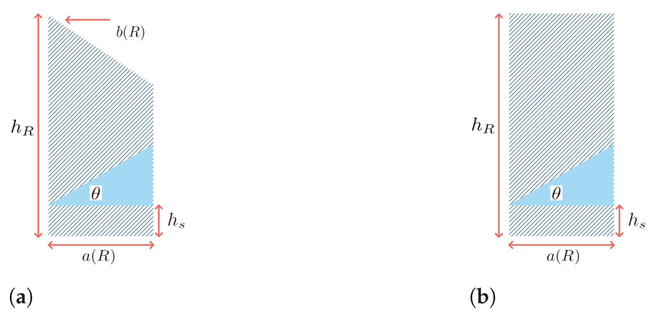
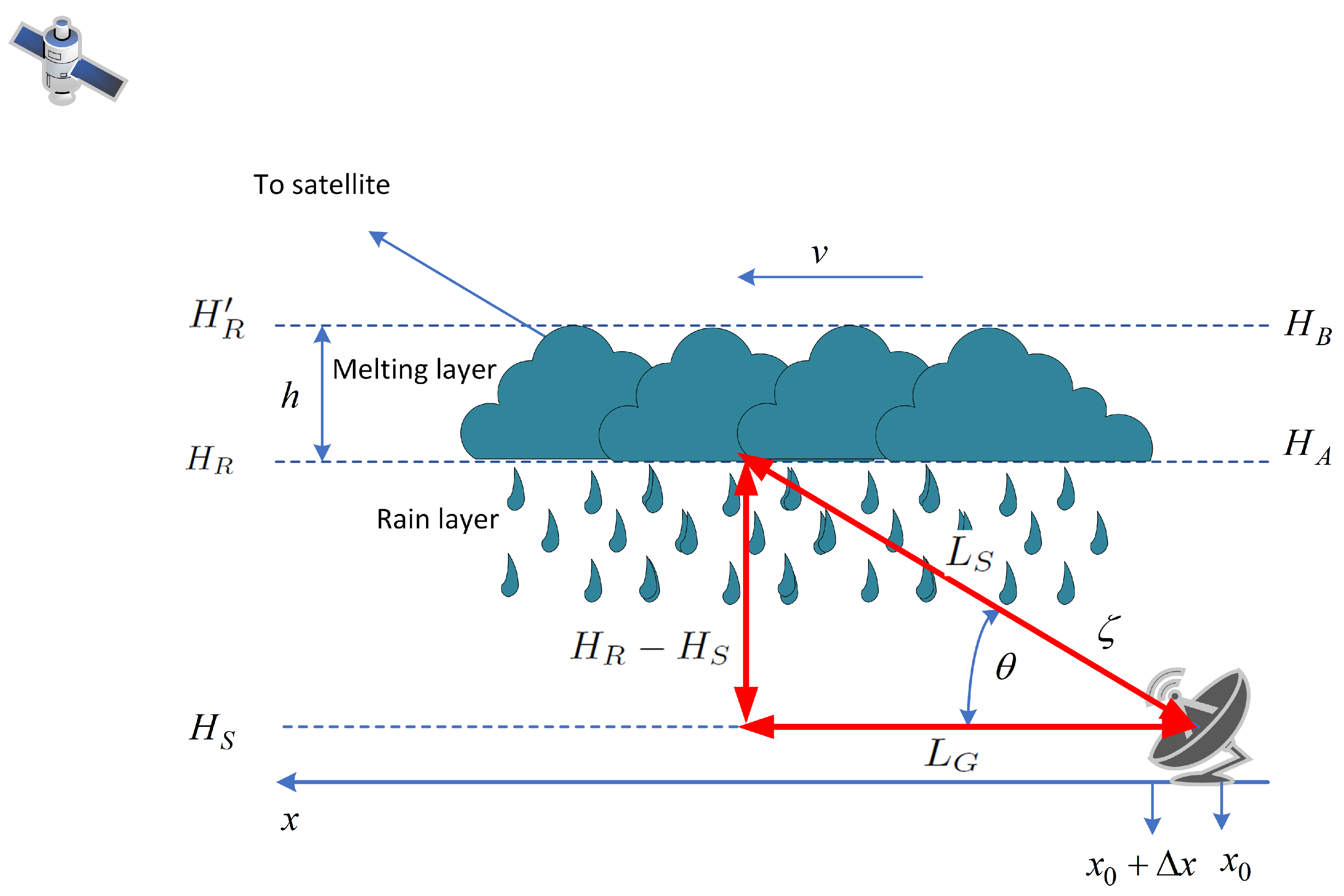
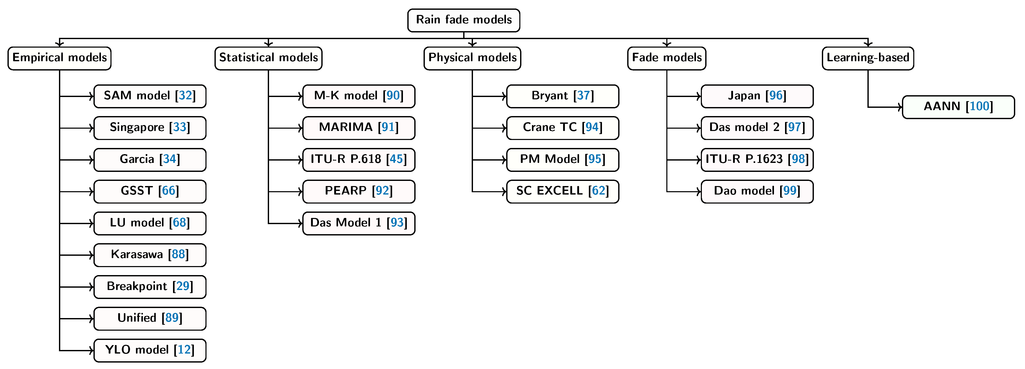
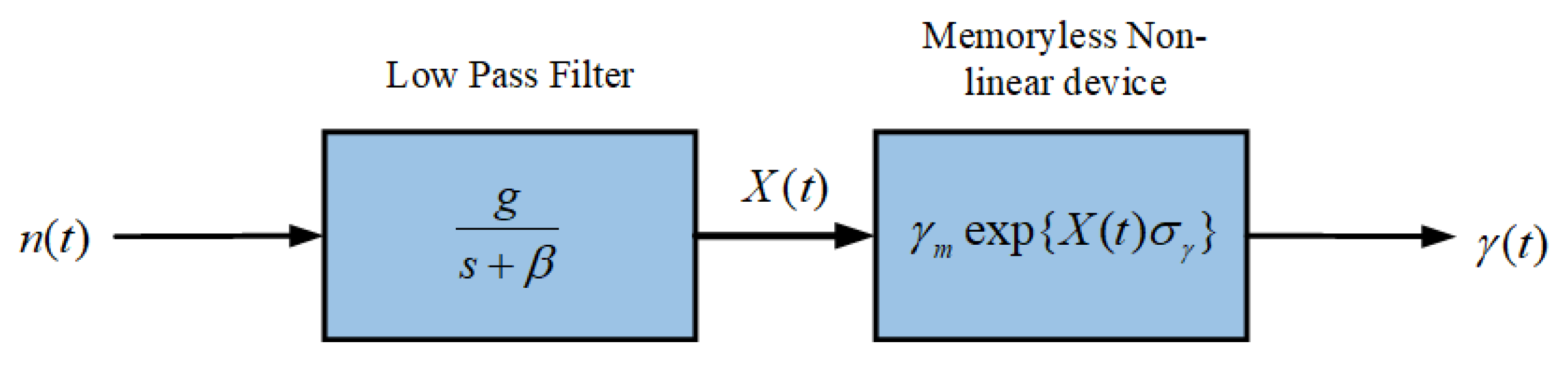
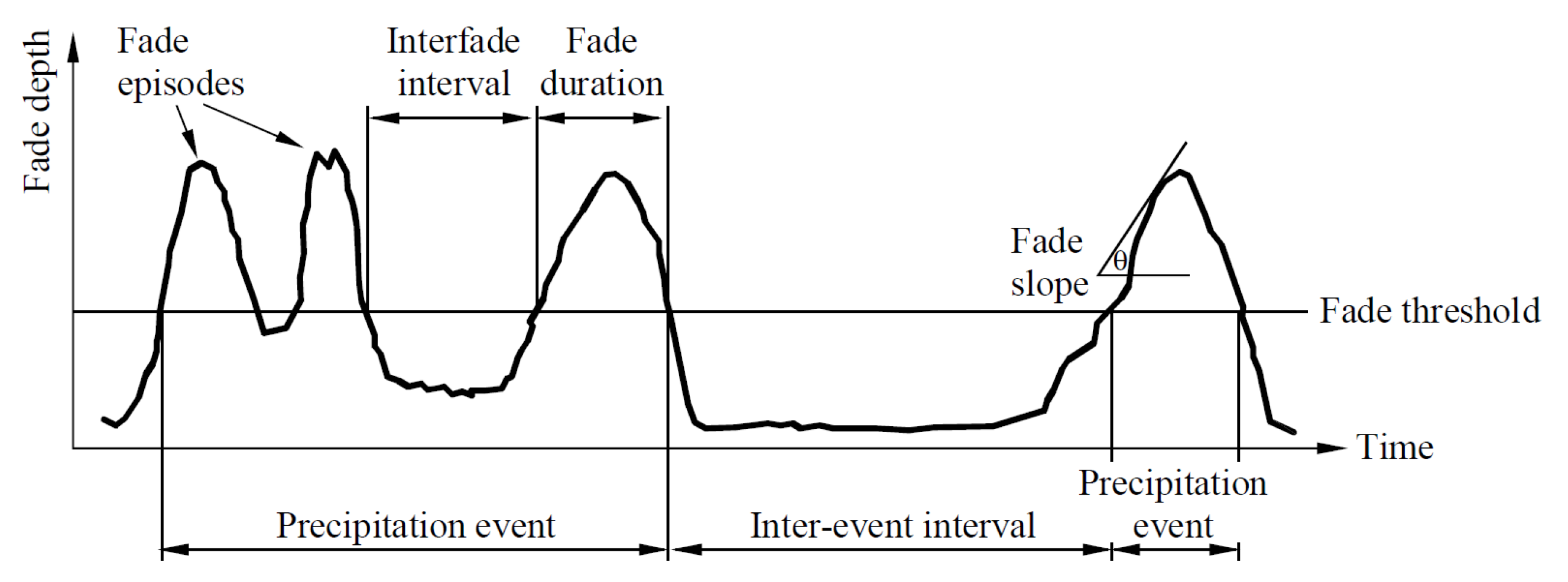
Table 1.
Rain attenuation survey papers.
| Ref. | Survey Concentrations |
|---|---|
| [14] | The results show that rain attenuation in horizontal polarization is slightly larger than that in vertical polarization. A differential coupling-based compensation was recommended to reduce the rain attenuation effects on polarization in the depolarization processes. |
| [15] | In this survey, the artificial-neural-network-based models were classified based on input parameters. In addition, the accuracy of the artificial-neural-network-based models was accessed through a comparative study. |
| [16] | Rain attenuation in a satellite system is more severe than in a terrestrial system, and for a good model, it should be implemented into the model through local climatic elements. |
Table 2.
Similarity and contrast between Earth–space to terrestrial links.
| Factors | Earth–Space | Terrestrial |
|---|---|---|
| Rain | ✓ | ✓ |
| Cloud, sky noise, scintillation, latitude, Earth radius | ✓ | ✗ |
| Hop length | Varies according to orbit:
| Varies according to necessity:
|
| Path length reduction | Effective slant path | Effective terrestrial path |
Table 3.
Different techniques to estimate rain height.
| Ref. | Mechanism | Symbol Meanings |
|---|---|---|
| [35] | is the isotherm height, and R is the rain rate. | |
| [36] | is the medium temperature, , under clear sky, and is under rainy condition temperatures, and is the specific attenuation coefficient. | |
| [37] | R is the rain rate in the range 30–70 mm/h. | |
| [38] | , also using rain height map | is the isotherm height. |
| [32] | is the latitude in degrees. | |
| [33] | is the latitude in degrees. | |
| [34] | is the latitude in degrees. | |
| [39] | R is the rain rate. | |
| [40] | R is the rain rate. | |
| [41] | is the latitude in degrees. |
Table 4.
Effective path length estimation techniques.
| Ref. | Mathematical Procedure |
|---|---|
| white [35] | , where R is the rain rate. |
| [42] | , where is the elevation angle, is the station height above mean sea level of the Earth, and is the horizontal projection length in the precipitation. |
| [43] | where is the projected path-length, which is defined by , a boundary rain rate. If then , and if then (Figure 1), and ‘’ is the effective number of rain cells given by , where , and ( is elevation angle). |
| [44] | The estimation of the rain path can be determined by calibrating the reflected signal in clear-sky conditions and in rainy conditions . Once rainfall events are identified the first step of the procedure involves the determination of the volume of the rain cell with . |
Table 5.
Rain rate conversion techniques.
| Ref. | Conversion Techniques |
|---|---|
| [49] | Using the Rain rate , where , the model can convert rain between 1- and -min, where is the probability that the mean rainfall rate is exceeded for a 1 min accumulation time, and is the probability that the mean rainfall rate is exceeded for min accumulation time. |
| [50] | Using cumulative rainfall distributions, the model can convert rain between 1- and -min. |
| [51] | Using the conversion factor , where () the model can convert 60 min to a 1 min integration time rain rate, where is the conversion factor, a, b, c, d are constants, and P is the probability of rainfall rate exceedance within . It can also be used to convert between different rain rates [52]. |
| [53] | Using the equation (), min to 1 min conversion. |
| [54] | Using the equation , where the model can convert the rain rate from min to 1 min. |
| [55] | Using the equation, , where : regression component determined statistically, and . |
| [56] | In the absence of accurate long-term rainfall data, this method takes the percent of time exceedance, latitude, and longitude as input to generate a 1 min integration time rain rate. |
| [57] | The model simply calculates the rain rate , where : maximum rainfall in mm for time interval T min. |
| [58] | , R: rain rate, u: empirical constant, a, b: depending on the location and integration time of the rain gauge. |
| [59] | where M is the average annual rainfall (mm), and T is the number of hours in the year during which rain rates exceed R (mm/h). |
| [60] | where p is the percentage of the time, M is the total annual rainfall accumulation, , and are constants, which can be derived from , and is the thunderstorm ratio (), where is the rain rate due to a thunderstorm and is the rain rate without a thunderstorm. |
| [61] | where R is the rain rate in mm/h and is the regional climatic parameter. |
Table 6.
Parameters of EXCELL model.
| Parameter | Monoaxial Rain Cell | Biaxial Rain Cell |
|---|---|---|
| Peak rainfall rate () | ✓ | ✓ |
| Cell radius/radii |
Table 7.
Characteristics table.
| Tpe | Ref. | Slant or Both | Rain Structure | Rainfall Rate | Frequency | Angle(Earth Station) | Rain Height | Melting Layer Height | Time Series |
|---|---|---|---|---|---|---|---|---|---|
| EMPI | [32] | Slant | ✓ | ✓ | ✓ | ✓ | ✗ | ✓ | ✓ |
| [33] | Slant | ✗ | ✓ | ✓ | ✓ | ✓ | ✗ | ✗ | |
| [34] | Slant | ✓ | ✓ | ✓ | ✓ | ✓ | ✗ | ✗ | |
| [66] | Slant | ✓ | ✓ | ✓ | ✓ | ✓ | ✓ | ✓ | |
| [68] | Slant | ✓ | ✗ | ✗ | ✗ | ✓ | ✓ | ✗ | |
| [88] | Slant | ✓ | ✓ | ✗ | ✓ | ✓ | ✗ | ✗ | |
| [29] | Slant | ✗ | ✓ | ✓ | ✓ | ✓ | ✗ | ✗ | |
| [89] | Both | ✗ | ✓ | ✓ | ✓ | ✗ | ✗ | ✗ | |
| [12] | Slant | ✗ | ✓ | ✓ | ✓ | ✓ | ✗ | ✗ | |
| STAT | [90] | Slant | ✗ | ✓ | ✓ | ✗ | ✗ | ✗ | ✗ |
| [91] | Slant | ✗ | ✓ | ✓ | ✓ | ✓ | ✗ | ✓ | |
| [45] | Slant | ✗ | ✓ | ✓ | ✓ | ✓ | ✗ | ✗ | |
| [92] | Slant | ✗ | ✓ | ✓ | ✓ | ✗ | ✗ | ✗ | |
| [93] | Slant | ✗ | ✗ | ✗ | ✗ | ✗ | ✗ | ✓ | |
| PHY | [37] | Slant | ✓ | ✓ | ✓ | ✓ | ✓ | ✗ | ✗ |
| [94] | Both | — | ✓ | — | ✓ | ✓ | ✗ | ✗ | |
| [95] | Both | ✓ | ✓ | ✗ | ✓ | ✓ | ✓ | ✓ | |
| [62] | Slant | ✓ | ✓ | ✓ | ✓ | ✓ | ✓ | ✗ | |
| FADE | [96] | Slant | ✗ | ✗ | ✓ | ✓ | ✗ | ✗ | ✗ |
| [97] | Slant | ✗ | ✗ | ✗ | ✗ | ✗ | ✗ | ✓ | |
| [98] | Slant | ✗ | ✗ | ✓ | ✓ | ✗ | ✗ | ✗ | |
| [99] | Slant | ✗ | ✗ | — | ✓ | ✗ | ✗ | ✗ | |
| LB | [100] | Slant | ✓ | ✓ | ✓ | ✓ | ✓ | ✓ | ✓ |
EMPI: empirical, STAT: statistical, PHY: physical, FADE: fade slope, LB: learning-based, k and , 5–50, 20–60, ground layer and melting layer, exponential rain cell, only rain height, no melting layer, 6.50 72.8. as is dependent on frequency (not polarization), mentioned but no mathematical form is found, rain attenuation is used, cylindrical rain cell, the rain structure is composed of heavy and light rainfall components, frequency parameter is not directly used in the calculation of the attenuation, as the applicable frequency range is limited to 10–50 GHz, not mentioned, s-constant that depends on elevation angle and climate.
Table 8.
Characteristics table.
| Type | Ref. | Frequency Range | Polarization | Regional Climatic Parameter | Spatial Friendly | Reported Region that Suits |
|---|---|---|---|---|---|---|
| EMPI | [32] | 10–35 GHz | ✓ | ✓ | ✓ | The USA, Europe, and Japan |
| [33] | 4–6 GHz | NM | Rainfall rate | ✗ | Singapore | |
| [34] | NM | ✓ | 4 coefficient constants called a,b,c and d depend on geographic area | NM | Best suited areas are in Europe, the USA, Japan, and Australia | |
| [66] | 10–100 GHz | ✓Circular, horizontal and vertical | Rainfall rate | ✗ | Temperate region | |
| [68] | Above 11 GHz | ✗ | Local rainfall rate | No information available | No practical information; test information is limited within DBSG3 databank | |
| [88] | 10–20 GHz | NM | Rainfall rate, the probabilities of occurrence and mean rainfalls, for cell and debris | The model considers a single volume rainfalling area and does not consider convective (cell) and stratified rain (debris) | CCIR rain zone | |
| [29] | 10.7–13 GHz (Ku band) | ✓ | Rainfall rate | NM | Fiji | |
| [89] | Terrestrial: 7–137 GHz | ✓k and | Rainfall rate | ✓ | Worldwide (ITU-R databank) | |
| [12] | 10–30 GHz | Both | Rainfall rate | ✗ | Tropical | |
| STAT | [90] | NM | ✓ | Rainfall rate | ✗ | Temperate region |
| [91] | 10–50 GHz | ✓ | Climate characteristics, link elevation angle | Has spatial dynamics of rainfall rate parameter due to Van de Kamp [127] | Xi’an, China | |
| [45] | Up to 55 GHz | ✓ | Rainfall rate | ✗ | Worldwide | |
| [92] | NM (only 20 GHz is mentioned) | NM | NM | Information NM | France | |
| [93] | NM | ✓Horizontal | Measured rain attenuation | NM | Kolkata, India | |
| PHY | [37] | Reported frequencies are 15, 30, 39.6 GHz | NM | ✓ | Rainfall rate is not a function of distance | Temperate and tropical |
| [94] | 1–100 GHz | ✗ | Cell and debris parameter | No spatial correlation function is included | Temperate region | |
| [95] | 11.6 GHz (Range NM) | ✓Circular, Linear | Rainfall rate, wind velocity | ✓(1-year rainfall rate PDF was used) | Italy | |
| [62] | 10–50 GHz | ✓ | Rainfall rate; rain height; melting layer height, etc. | ✓Vertical and horizontal | Worldwide | |
| FADE | [96] | Ku-band | RHCP, Linear polarization | ✗ | ✗ | Japan (low-elevation Earth–space path) |
| [97] | NM | Horizontal | ✓ | ✗ | Tropical area | |
| [98] | 10–50 GHz | NM | ✓ | ✗ | Designed for global perspective | |
| [99] | 10.982 GHz (Ku-band) | Vertical | s-parameter | ✗ | Malaysia | |
| LB | [100] | NM | NM | Local rainfall data: it needs to train the BPNN networks | NM | Butare, Rwanda |
EMPI: empirical, STAT: statistical, PHY: physical, FADE: fade slope, LB: learning-based rain attenuation model, not mentioned, elevation angle, s-parameter definition is given in Equation (60).
Table 9.
Characteristics table.
| Type | Ref. | Used/Validation Databank | Remarks about Validation | Complexity Level | Constraints |
|---|---|---|---|---|---|
| EMPI | [32] | 62 experiments in the USA, Japan and Europe | Shows better prediction with minimum 2 years rainfall datasets | low | The operating frequency range is limited to 10–35 GHz |
| [33] | INTELSAT POR experiment (Singapore) | The results have been validated with CCIR model and measured attenuation | low | The recommended frequency is limited to 4–6 GHz | |
| [34] | 77 satellite links placed in Europe, the USA, Japan, and Australia (CCIR data bank) | Validated by the author | low | The model is suitable for prediction with an elevation angle ranging from 10 to 40 | |
| [66] | ITU-R databank | ITU-R databank is used to examine the behavior of m parameter at different frequencies as well as different sites | low | Not spatial friendly | |
| [68] | DBSG3 databank | The RMS value show that the new model provides the smallest rms and STD in all percentages of time except at 0.001% | high | Application area is limited by low latitudes (between 36 South and 36 North) and low elevation angles (25<) | |
| [88] | CCIR rain zone with different elevation angle | Validated by the author | medium ∔ | 10–20 GHz | |
| [29] | Used 6 tropical city’s rain databanks from ITU-R | The experimental result agreed about correction factor induced attenuation especially at elevation angle less than 60 compared to ITU-R model | medium | In this model it is assumed that rain is uniformly distributed inside a rain cell | |
| [89] | ITU-R databank | The model gives decent results with the correctness of its terrestrial and slant direction | medium | The model was not checked with actual data for attenuation | |
| [12] | ✗ | Verified with the the beacon signals from WINDS and GE23 satellites (2009 to 2012) | low | Up to 30 GHz frequency is examined | |
| STAT | [90] | ✗ | Not validated with heavy rainfall or with rainfall data around the world for different sites | low | The model is applicable only during the rain periods because no transition is included in the model to switch from rainy to clear sky conditions |
| [91] | Validated based on the measured rain attenuation data at Xi’an, China | The validation is a good agreement between measured and predicted attenuation using this model, but has not been compared with other important rain attenuation models | high | The size of the area is not defined for a specific set of parameters | |
| [92] | ✗ | Not validated | — | The probabilistic weather forecasts could be beneficial to maximize the economic value accounting the transmitted data for higher frequencies (say 50 GHz). | |
| [93] | ✗: used measured attenuation data | The validation shows a good agreement between measured and predicted attenuation using this model, but has not been compared with other important rain attenuation models | medium | It needs to derive mean and standard deviation of the Gaussian distribution for a different geographic area and find the coefficients of second-order polynomials from real measured attenuation | |
| PHY | [37] | ✓ | Validated at Lae, Papua New Guinea | low | — |
| [94] | Satellite: validated through CCIR procedure. Terrestrial: 35 terrestrial paths around the world | Both satellite and terrestrial links have been verified | high | The probabilities of incidence and mean precipitation for cells and debris are difficult to determine | |
| [95] | Experimental dataset | The experimental results show that the method show less error probability. | medium | Needs 1 min rainfall rate | |
| [62] | DBSG3 databank | Although the model does not outperform the existing ITU-R model (approximately 2.4% error), it supports a few additional facilities (e.g., site diversity) and takes account of the interference due to hydrometer scattering | high | The correctness is limited by the local values of input parameters like the melting layer and the rain plateau value, which might not be available everywhere | |
| FADE | [96] | Experimental dataset | Validated with | low | — |
| [97] | ✗ | Validated in Kolkata, India, with experimental set-up | low | To use fade margin data it needs to remove tropospheric scintillation | |
| [99] | Only experimental dataset | The resulted output agrees with the measured standard deviation of attenuation | low | The method was tested only at 10.982 GHz | |
| [98] | NM | Validated in [140,141] | low | Applicable for limited elevation angle 5–60 | |
| LB | [100] | Durban, South Africa | The model was not validated with standard DSDB3 or CCIR rain databanks | — | The model was not tested with established well-known rain databanks like DBSG3 or CCIR |
EMPI: empirical, STAT: statistical, ∔ it needs to solve at least seven equations. PHY: physical, FADE: fade slope, LB: learning-based rain attenuation model, † it needs to solve ten equations.
Publisher’s Note: MDPI stays neutral with regard to jurisdictional claims in published maps and institutional affiliations. |
© 2021 by the authors. Licensee MDPI, Basel, Switzerland. This article is an open access article distributed under the terms and conditions of the Creative Commons Attribution (CC BY) license (https://creativecommons.org/licenses/by/4.0/).
Share and Cite
MDPI and ACS Style
Samad, M.A.; Diba, F.D.; Choi, D.-Y. A Survey of Rain Fade Models for Earth–Space Telecommunication Links—Taxonomy, Methods, and Comparative Study. Remote Sens. 2021, 13, 1965. https://doi.org/10.3390/rs13101965
AMA Style
Samad MA, Diba FD, Choi D-Y. A Survey of Rain Fade Models for Earth–Space Telecommunication Links—Taxonomy, Methods, and Comparative Study. Remote Sensing. 2021; 13(10):1965. https://doi.org/10.3390/rs13101965
Chicago/Turabian StyleSamad, Md Abdus, Feyisa Debo Diba, and Dong-You Choi. 2021. "A Survey of Rain Fade Models for Earth–Space Telecommunication Links—Taxonomy, Methods, and Comparative Study" Remote Sensing 13, no. 10: 1965. https://doi.org/10.3390/rs13101965
Note that from the first issue of 2016, this journal uses article numbers instead of page numbers. See further details here.