Wave-Filtered Surf Zone Circulation under High-Energy Waves Derived from Video-Based Optical Systems

Abstract

This paper examines the potential of an optical flow video-based technique to estimate wave-filtered surface currents in the nearshore where wave-breaking induced foam is present. This approach uses the drifting foam, left after the passage of breaking waves, as a quasi-passive tracer and tracks it to estimate the surface water flow. The optical signature associated with sea-swell waves is first removed from the image sequence to avoid capturing propagating waves instead of the desired foam motion. Waves are removed by applying a temporal Fourier low-pass filter to each pixel of the image. The low-pass filtered images are then fed into an optical flow algorithm to estimate the foam displacement and to produce mean velocity fields (i.e., wave-filtered surface currents). We use one week of consecutive 1-Hz sampled frames collected during daylight hours from a single fixed camera located at La Petite Chambre d’Amour beach (Anglet, SW France) under high-energy conditions with significant wave height ranging from 0.8 to 3.3 m. Optical flow-computed velocities are compared against time-averaged in situ measurements retrieved from one current profiler installed on a submerged reef. The computed circulation patterns are also compared against surf-zone drifter trajectories under different field conditions. Optical flow time-averaged velocities show a good agreement with current profiler measurements: coefficient of determination $\left(r^2\right)=$ 0.5–0.8; root mean square error $\left(\mathrm{RMSE}\right)$ = 0.12–0.24 m/s; mean error (bias) $=-0.09$ to $-0.17$ m/s; regression slope $=1\pm 0.15$; ${\mathrm{coherence}}^2$ = 0.4–0.6. Despite an underestimation of offshore-directed velocities under persistent wave breaking across the reef, the optical flow was able to correctly reproduce the mean flow patterns depicted by drifter trajectories. Such patterns include rip-cell circulation, dominant onshore-directed surface flow and energetic longshore current. Our study suggests that open-source optical flow algorithms are a promising technique for coastal imaging applications, particularly under high-energy wave conditions when in situ instrument deployment can be challenging.

1. Introduction

Currents induced by wave breaking constitute the primary driving mechanism of sediment transport and morphological change in the nearshore [1]. Currents flowing along the shore (longshore currents) have the capacity to transport hundreds of thousands of cubic meters of sand per year, reshaping the underlying bathymetry and mobilizing nutrients, pollutants and biological species [2,3]. Wave action in the breaker zone induces a net transport of water toward the shore, however, at certain locations along the coastline, the water returns seawards through relatively narrows zones as rip currents [4]. Rip currents are concentrated fast-moving flows of water that extend from close to the shoreline through the surf zone, sometimes beyond the breaking region [5]. These seaward-directed currents can pull swimmers offshore into deeper water making them the leading cause of fatal drowning and lifeguard rescues on beaches worldwide [6]. Rip currents and associated surf-zone circulations are subject to tidal and wave group modulation as well as to local bathymetry variations making them highly variable in space and time, with flow pulsing within the infragravity (0.004–0.04 Hz) and very low frequency (VLF) band (<0.004 Hz) [7,8]. In this context, characterizing the nearshore circulation system is crucial for efficient coastal infrastructure planning, reliable environmental assessment and appropriate beach safety strategy.

Traditional nearshore surf-zone velocity measurements are obtained by instruments deployed in situ collecting Eulerian or Lagrangian data. Examples of these instruments are electromagnetic current meters, acoustic sensors, and surface drifters [9,10]. Although these measuring techniques are robust and accurate, they are usually limited to punctual measurements over short durations [11]. Moreover, the deployment and periodic maintainence of the instruments require a significant amount of money, manpower and logistics resources [12]. Overall, collecting Eulerian and particularly Lagrangian data in high-energy beach environments is one of the greatest challenges [5]. In order to overcome these limitations, remote sensing provides an attractive alternative.

Over the past decades, the use of low-cost shore-based video systems and more recently camera-equipped unmanned aerial vehicles (UAVs) have enabled access to high-resolution temporal and spatial data of the water surface layer [13,14,15]. A few approaches based on optical remote sensing techniques have been developed to identify and characterize local surface currents associated with specific frequency bands. Dispersion relation fitting techniques [12,16,17] are one of such methods. Using the Doppler shifting of the surface gravity wave field, the surface velocity vector is estimated from the difference between observed wave phase velocity and that given by the linear dispersion relation [17]. However, the use of the linear wave dispersion in the nearshore region is questionable since non-linear effects in wave hydrodynamics become significant for example, see [18]. Moreover, the method requires a strong optical signature from the waves, which becomes problematic in the surf zone due to the presence of foam and broken waves.

Alternatively, the presence of foam have actually been exploited by optical tracking algorithms to estimate the surface flow velocity and the propagation speed of (broken) wave crests [3,11,19,20,21,22]. In the case of low wind, the remnant foam produced by breaking waves is assumed to act as a quasi-passive tracer being advected only by the underlying currents as long as the passing waves are removed. This assumption has been exploited to estimate mean longshore currents in the surf zone along a transect of pixels parallel to the shore [3,11].

For extraction of the two-dimensional velocity field, perhaps the most common and well-documented video-based technique is particle image velocimetry (PIV) [23,24]. This method essentially splits the image into several user-defined image segments or windows. The spatially-averaged displacement of a cluster of particles inside each window is computed over time using a cross-correlation approach. PIV-based techniques are typically performed in laboratory conditions using particle images (fluids containing reflective and neutrally buoyant tracer particles) to determine the velocity of the flow [25,26]. Nevertheless, several studies have applied the PIV-based approach using shore-based and UAV video footage to estimate bore celerities and surface currents in the nearshore (surf zone and swash zone) [19,20,27,28,29,30,31].

An alternative video-based technique that estimates the velocity field between consecutive images are optical flow algorithms [32]. Dérian and Almar [21] presented a methodology based on an optical flow algorithm named “Typhoon” capable to estimate instantaneous nearshore surface currents from image sequences. More recently, Anderson et al. [22] presented a new technique for processing surf-zone imagery called WAMFlow. Their approach consists of filtering the dominant optical clutter of incident waves from an image sequence by averaging frames over a sliding window in time with size of twice the dominant wave period. The resulting wave-averaged movie (WAM) contains residual foam features which are tracked using an optical flow algorithm to estimate the underlying mean flow motion inside the surf zone.

This paper builds on Anderson et al. [22] similar wave-averaged approach. However, an alternative technique is proposed to remove the dominant wave optical signature present in the image sequence based on the use of a temporal Fourier low-pass filter. The present paper aims to compare for the first time optical flow-derived velocities against in situ velocity measurements from a fixed bottom-mounted Acoustic Doppler Current Profiler (ADCP). Optical flow estimates are also qualitatively compared with Lagrangian drifters deployed at the southern end of Anglet beach (Basque Coast, SW France) during an intensive field experiment carried out in October 2018 under different wave, tide and wind conditions. Furthermore, this study provides some standard parameters for Liu [33] MATLAB open-source optical flow program (“OpenOpticalFlow”) so that anyone can reproduce and estimate wave-filtered surface velocity fields within the surf zone from consecutive images.

This paper is organized as follows: A brief introduction of the optical flow algorithm, as well as the physics-based equations, are detailed in Section 2. The study site and the field experiment, including all available instruments, are described in Section 3. The main processing steps before and after optical flow implementation are introduced in Section 4. Results, performance and limitations of the optical flow method are presented in Section 5 and further discussed in Section 6 before conclusions are drawn in Section 7.

2. Optical Flow Algorithm

Optical flow can be described as the apparent motion of individuals pixels (i.e., brightness patterns) between consecutive frames on the image plane [32,34]. The present optical flow method is a differential approach based on a global formulation with a smoothness constraint which is capable to estimate the entire vector flow field simultaneously by solving a single equation [21,33]. The estimated pixel displacement and the known time interval between frames allow computing 2D velocity components within the entire image domain. The underlying assumption is that the image intensity from one frame to another remains invariant such that the time derivative of the image intensity can be accurately evaluated [35]. This holds under the hypothesis that the pixel displacement is sufficiently small so that the pixel intensity remains constant [32].

We used Liu [33] MATLAB open-source optical flow program (“OpenOpticalFlow”) to extract high-resolution velocity fields from an image sequence containing continuous patterns. The physical and mathematical foundations of Liu [33] optical flow method are well established and have been validated for various fluid flow visualizations using laboratory, cloud and ocean images [35,36,37]. The physics-based optical flow equation in image coordinates is given by:

$$\frac{\partial I}{\partial t}+\nabla ·\left(I\mathbf{u}\right)=f(x_1,x_2,I),$$

(1)

where I is the normalized image pixel intensity, $\mathbf{u}=\left(u_1,u_2\right)$ is the velocity vector with $\left(x_1,x_2\right)$ coordinates in the image plane referred to as the optical flow and $f(x_1,x_2,I)$ is related to the boundary term and diffusion term. $\nabla ·$ is the divergence operator and $\nabla =\left(\frac{\partial }{\partial x_1},\frac{\partial }{\partial x_2}\right)$ is the spatial gradient. Equation (1) is a generic form of the projected-motion equations derived by Liu and Shen [36] where the optical flow $\mathbf{u}$ is proportional to the path-averaged velocity of fluid or particles in flow visualizations. Equation (1) is treated as an inverse problem since it is one equation with two unknowns $(u_1,u_2)$. To determine the optical flow, a variational formulation with a first-order smoothness constraint is typically used [32,36]. Given I and f, we define a functional:

$$J\left(\mathbf{u}\right)={\int }_{\Omega }{\left[\frac{\partial I}{\partial t}+\nabla ·\left(I\mathbf{u}\right)-f\right]}^{2}d{x}_{1}d{x}_2+\lambda {\int }_{\Omega }\left(|\nabla u_1{|}^2+{|\nabla u_2|}^2\right)d{x}_{1}d{x}_2,$$

(2)

where $\lambda$ is the Lagrange multiplier and $\Omega$ is the image domain. Minimization of the functional $J\left(\mathbf{u}\right)$ leads to the Euler-Lagrange equation:

$$I\nabla \left[\frac{\partial I}{\partial t}+\nabla ·\left(I\mathbf{u}\right)-f\right]+\lambda {\nabla }^2\mathbf{u}=0,$$

(3)

where ${\nabla }^2=\left(\frac{{\partial }^2}{\partial x_1^2}+\frac{{\partial }^2}{\partial x_2^2}\right)$ is the Laplace operator and $\lambda$ is the Lagrange multiplier that controls the smoothness of the field. In the special case where $\nabla \mathbf{u}=0$ and $f=0$, Equation (1) reduces to the Horn and Schunck [32] brightness constraint equation:

$$\frac{\partial I}{\partial t}+\mathbf{u}·\nabla I=0,$$

(4)

and further to the Euler-Lagrange equation originally given by Horn and Schunck [32]:

$$\left[\frac{\partial I}{\partial t}+\mathbf{u}·\nabla I\right]\nabla I-\lambda {\nabla }^2\mathbf{u}=0.$$

(5)

Equations (3) and (5) are solved using the standard finite difference method with the Neumann condition $\frac{\partial \mathbf{u}}{\partial n}=0$ on the image domain boundary $\partial \Omega$ [36,38]. In computations, the solution of Equation (5) is used as an initial approximation for Equation (3) for faster convergence. The subroutines inside OpenOpticalFlow [33] in charge of solving Equations (3) and (5) are “horn_schunck_estimator.m” and “liu_shen_estimator.m”, respectively. Further details on the mathematical development and error analysis of the optical flow method can be found in [33,36,37,38].

Liu [33] OpenOpticalFlow program also includes additional subroutines for image pre-processing (e.g., Gaussian filter for local illumination correction and random noise removal) and a coarse-to-fine iterative scheme for improvement of the optical flow computation in case of large pixel displacements. A brief description of the relevant input parameters is presented in Appendix A and can be found in Liu [33].

3. La Petite Chambre d’Amour Beach Experiment

3.1. Study Site

La Petite Chambre d’Amour (PCA) beach is the most southern stretch of the 4-km long sandy embayment of Anglet beach located on the Basque Coast, SW France (Figure 1). PCA beach is bounded by a prominent 500-m long rocky headland in the South and comprises a 90-m groin in the North. These two morphological characteristics play an important role on the beach state and rip current location [39]. Close to the headland, a 20-m wide submerged rocky reef is present exerting persistent wave breaking and occasionally bathymetrically-controlled rips at low tide under low-energy waves [40]. The beach is composed of medium to coarse sand ($D_{50}\approx 2$ mm) and is classified as a high-energy intermediate beach with the presence of a double-bar (occasionally single-bar) system [39]. The relative steep beach face ($tan\beta \approx 1/10$) favors the formation of beach cusps with shoreline dynamics strongly controlled by the geometry of the surf-zone sandbar [41]. The coast is predominantly exposed to Atlantic W-NW high-energy incoming swells with an average annual offshore significant wave height $H_s=1.57$ m (up to 10 m during winter storms) and average peak wave period $T_p=10$ s [42]. The tide is semi-diurnal characterized by a meso-macro tidal regime with an average range varying between 1.69 m (for neap tides) and 3.94 m (for spring tides) [43]. Breaking waves are the dominant driver of nearshore currents, with tide elevation affecting breaking patterns and in turn modulating nearshore currents [44]. As opposed to the northern Aquitaine open sandy beaches, PCA beach responds predominantly at individual storm frequency rather than at seasonal timescales [39].

3.2. Field Experiment

An intensive field campaign was performed at PCA beach from 3 to 26 October 2018 with the objective to investigate the nearshore current circulation and headland flows under a range of energetic wave conditions [45]. The 3-week field experiment involved a large display of instruments including four Acoustic Doppler Current Profilers (ADCPs), six surf-zone drifters and high-frequency video monitoring from a fixed video-camera and a camera-equipped UAV. In-situ directional wave and wind measurements were also continuously collected (every 30 min and 1 h, respectively) by a permanent directional wave buoy located approximately 6 km offshore and by the Biarritz airport meteorological station (71 m altitude) located 3 km SE of the study site, respectively. Hourly water level measurements were retrieved from Saint-Jean-De-Luz tide gauge located 15 km SW of the study site. In the frame of the large-scale field experiment described in Mouragues et al. [40], the present dataset gathers the data collected during the longest continuous fixed-camera video recording (8–15 October 2018) together with simultaneous Eulerian measurements collected from a single available ADCP installed over the submerged reef within the camera view field (Figure 1). The field conditions during this week are shown in Figure 2 and are described in the following subsection. In addition, the present study examines simultaneous video and drifter data during four days (on 18, 19, 22 and 23 October 2018) under different wave, wind and tide conditions (

Table 1. Field conditions during the four days of drifter deployments. Offshore peak wave angle of incidence (${\theta }_p$) and wind direction incidence are relative to the shore normal.

	18 October 2018	19 October 2018	22 October 2018	23 October 2018
Time [GMT]	11:52 to 13:57	07:26 to 10:28	07:42 to 10:34	08:02 to 08:35	08:36 to 11:38
Configuration	Shore-normal	Shadowed	Shore-normal	Deflection	Deflection
Drifter Deployments	16	28	46	5	30
${\mathit{H}}_{\mathit{s}}$ [m]	1.9	1.6	1	1.7	1.6
${\mathit{T}}_{\mathit{p}}$ [s]	14	13	11	13	11
${\mathit{\theta }}_{\mathit{p}}$ [°]	0	−5	0	4	8
Wind Speed [m/s]	2.4	1.1	3.6	0.6	1.7
Wind Direction [°]	10	−50	30	−180	140
Tide Stage	Ebb	Flood	Flood	Ebb	Flood
Water Level Range [m]	0.66 to 0.08	−0.42 to 0.58	−1.49 to −0.46	−1.70 to −1.74	−1.75 to −0.13

).

3.2.1. Field Conditions and Overall Nearshore Circulation

The 1-week (8–15 October 2018) continuous set of measurements used in this study (Figure 2) builds on the same experiment presented by Mouragues et al. [40]. Overall, PCA beach was exposed to relatively energetic offshore wave conditions (average $H_s=1.6$ m) with high-energy wave events ($H_s>2$ m) with peak wave period $T_p$ ranging from 7 to 15 s (Figure 2a,b). Offshore wave conditions also featured a wide range of wave angle of incidence ($-23<{\theta }_p<20$°; Figure 2c). The sign of the peak wave incidence ${\theta }_p$ (angle of wave incidence relative to the shore normal) indicates on which side of the headland waves were coming from. Wind conditions (Figure 2d,e) were relatively weak with mean wind speed values around 3 m/s coming primarily from the S-SE sector. A single moderate wind event was captured on 14 October 2018, reaching wind speed up to 12 m/s coming from the W-NW (roughly shore normal) direction. During the field experiment, PCA beach morphology corresponded to a low-tide terrace beach state (Wright and Short [46] classification) with a mostly alongshore-uniform sandy bed that barely evolved throughout the experiment. The reader is referred to Mouragues et al. [40,45] for more information about PCA bathymetry details.

Mouragues et al. [40] classified wave-induced circulation patterns observed at PCA into three wave angle of incidence configurations. According to this classification, the 1-week dataset was identified as a deflection (${\theta }_p>0$°; 8–10 October 2018), shore-normal (${\theta }_p=0$°; 11 October 2018) and shadowed (${\theta }_p<0$°; 12–15 October 2018) configuration. During deflection configuration (8–10 October 2018), the ADCP captured longshore currents flowing toward the headland (Figure 2f). The seaward deflection of the longshore current against the headland produced deflection rips with offshore surface velocities sporadically exceeding 0.4 m/s. On the single day of shore-normal configuration (11 October 2018) the surface flow was characterized by cross-shore motions with surface velocities oscillating between −0.4 and 0.4 m/s. During the shadowed regime (12–15 October 2018) surface currents were primarily onshore directed flowing away from the headland driven by alongshore variations in wave breaking induced by the shadowing effect of the headland [5]. Overall, surface currents were found to be strongly modulated by the tide, which coincided with a spring tide cycle with the water depth column varying from 1.5 to 5.9 m at the location of the ADCP (gray shaded region in Figure 2f). As opposed to open sandy beach embayments, PCA beach inherited geological features (headland and submerged reef) exert a strong control on nearshore circulation. A close inspection of the time evolution of wave breaking water depth, defined as $h_{br}=H_s/0.5$ for PCA field site, indicates that the ADCP is within the outer edge of the surf zone only around low tide for $H_s<2$ m (red line in Figure 2f). Therefore, the submerged reef (where the ADCP is installed) is assumed to play a major control in flow dynamics as waves start to break over the reef when water depth decreases.

In the frame of the drifter experiment described in Mouragues et al. [40], four days of drifter deployments were selected to analyze PCA beach main circulation patterns under different oblique wave configurations with varying wave, wind and tide conditions (Table 1). In particular, during the rising neap low tide on 23 October 2018, a deflection rip was found to systematically advect drifters from the surf zone to at least 1000 m offshore. The spatial structure of the rip consisted of an approximately 150-m wide rip neck along the headland with a wider rip head extending further offshore the headland. Lagrangian and Eulerian measurements registered mean surface velocities around 0.3 m/s in the rip neck and 0.35 m/s in the rip head along with VLF rip pulsations with characteristic periods around 30 and 50 min [40,44].

3.2.2. Video Data

High-frequency sampled images (1 Hz) recorded at 1624 × 1234 px were collected from a single permanent camera video station installed on the top of Biarritz lighthouse (70 m above mean sea level) located near the tip of the headland (green star in Figure 1). The resulting oblique images covered part of PCA near the headland, including the submerged reef and the surf zone. Unfortunately, only one of the four ADCPs deployed during the experiment was within the camera view field. In order to compare optical flow derived velocities against in-situ instruments, one week of continuous daylight video recording corresponding to simultaneous ADCP measurements were selected from 8 October 2018—07:00:00 to 15 October 2018—15:30:00 GMT. Moreover, Lagrangian measurements together with simultaneous video data were used to provide a spatial insight of the surface flow. Drifter trajectories were captured by the video system on four different days. Between 2 and 3.5-h burst of images were selected from each day of drifter deployment for further post-processing and analysis.

3.2.3. ADCP Data

A single ADCP (Nortek Aquadopp Profiler 2 MHz) was deployed within the fixed camera view field approximately 280 m away from the video station (Figure 1). This ADCP was used to retrieve current measurements to further validate optical flow surface velocities. The ADCP was mounted horizontally on an AquaCross aluminum frame (Figure 3) near the bottom of the submerged rocky reef between 1.5–5.9 m depth (depending on the tide elevation) and 1-Hz continuous measurements of pressure and velocities along the water column were collected during 1 week (8–15 October 2018) for optical flow comparison. The pressure sensor was located 0.2 m above the seabed (${\delta }_s$). The velocity profile was measured over vertical cells ($z_{cell}$) of 0.1 m size (${\delta }_c$ = cell size) after a blanking distance (${\delta }_b$) of 0.1 m from the instrument. Velocity measurements were assigned to the center of each cell starting with the bottom cell at 0.35 m ($z_{cel{l}_1}={\delta }_s+{\delta }_b+{\delta }_c/2$; Figure 3) above the sand bed.

Direct comparison of remotely sensed currents with fixed in situ instruments is not a trivial task [21,22]. Video-derived velocities are extracted from the time-varying water surface layer which is locally influenced by instantaneous wave and wind conditions. On the other hand, conventional ADCPs typically discard data from the upper region of the water column leading to an inevitable spatial mismatch for a true velocity comparison. Upper cells emerge intermittently at the passage of a wave trough restricting the analysis within the water column below this elevation [44]. To overcome this limitation, we make use of the concept of $\sigma$-layers, which will be described below.

According to the shallowness parameter $\mu$, the water surface at the location of the ADCP was characterized by weakly dispersive waves propagating in shallow waters ($\mu \approx 0.12$). The shallowness parameter $\mu$ is defined as:

$$\mu ={\left(h_{0}k\right)}^2,$$

(6)

where $h_0$ is the mean water depth and k the typical wave number ($k\approx 0.08$ 1/m). The pressure was used to reconstruct the water surface elevation using Bonneton et al. [47] non-linear shallow water reconstruction formula, valid for weakly dispersive waves propagating in the shoaling and surf zone (see [48,49]):

$${\zeta }_H=\frac{P_s-P_{atm}}{\rho g}-h_0+{\delta }_s,$$

(7)

$${\zeta }_{SL}={\zeta }_H-\frac{h_0}{2g}\left(1-{\left(\frac{{\delta }_s}{h_0}\right)}^2\right)\frac{{\partial }^2{\zeta }_H}{\partial t^2},$$

(8)

$${\zeta }_{SNL}={\zeta }_{SL}-\frac{1}{g}\left(\frac{\partial }{\partial t}\left({\zeta }_{SL}\frac{\partial {\zeta }_{SL}}{\partial t}\right)-{\left(\frac{{\delta }_s}{h_0}\right)}^2{\left(\frac{\partial {\zeta }_{SL}}{\partial t}\right)}^2\right),$$

(9)

where ${\zeta }_H$ is the hydrostatic reconstruction, ${\zeta }_{SL}$ the linear shallow water reconstruction, ${\zeta }_{SNL}$ the non-linear shallow water reconstruction above the mean water level, $\frac{{\partial }^2}{\partial t^2}$ the second-order time derivative, $\rho$ the water density, g the gravity, $P_s$ the pressure measured at distance ${\delta }_s$ above the bottom and $P_{atm}$ the (constant) atmospheric pressure. The reconstructed water depth is defined as:

$$h_{SNL}=h_0+{\zeta }_{SNL}.$$

(10)

For this study, the mean water depth $h_0$ and the reconstructed water surface ${\zeta }_{SNL}$ were computed consecutively over ∼17-min segments throughout the whole time series. ADCP cells above the reconstructed water surface were discarded from the analysis and submerged cells were depth-normalized. ADCP horizontal velocities along the water column were transformed to a vertical $\sigma$ coordinate system in order to measure the velocities close to the water surface consistent with video-camera derived optical flow estimation (see Figure 3). In addition, ADCP depth-averaged velocities were also computed for comparison with optical flow estimates. The $\sigma$ coordinate system is expressed by a user-defined number of vertical layers m, hereafter referred to as $\sigma$-layers. Each $\sigma$-layer j is normalized by the distance between the first ADCP cell and the instantaneous water surface elevation:

$${\sigma }_j=\frac{\left(j-1\right)\Delta z-z_{cel{l}_1}}{h_{SNL}-z_{cel{l}_1}};j=1,2,3,\dots ,m;\Delta z=\frac{h_{SNL}-z_{cel{l}_1}}{m-1}.$$

(11)

The first sigma layer (${\sigma }_1$) corresponding to the near-bottom is equal to zero and the last sigma layer corresponding to the water surface (${\sigma }_m$) is equal to one. ADCP vertical cells $z_{cel{l}_i}$ are interpolated to each $\sigma$-layer ${\sigma }_j$ before normalization. Regardless of the water depth, $\sigma$-layers are constrained to be equally divided along the water column so their individual value in terms of sigma (between 0 and 1) remains constant, whereas the thickness between $\sigma$-layers ($\Delta z$) in terms of meters is varying at each time step. $\sigma$-layers coincide with the irregular water wave surface within the water column and allow the calculation of residual velocity around the mean water surface level [50,51]. For the present study, 21 $\sigma$-layers were defined where each layer corresponded to 5% of the instantaneous water column. Moreover, the three $\sigma$-layers closest to the water surface were averaged (${\sigma }_{19}$, ${\sigma }_{20}$ and ${\sigma }_{21}$) and are hereafter referred to as the ADCP surface velocity measurements. Similarly, all the 21 $\sigma$-layers were averaged and are hereafter referred to as the ADCP depth-averaged velocity measurements.

3.2.4. Drifter Data

Six GPS-tracked surf-zone drifters were released multiple times on four different days (on 18, 19, 22 and 23 October 2018) with the purpose of providing greater spatial coverage of rip cell circulation. Deployments lasted from 2 to 3.5 h (Table 1). Drifters were individually seeded over the submerged reef region using a jet ski or by swimmers under reasonably safe conditions. Drifters’ positions logged at 2.5 Hz were locally stored on an SD card and transmitted in real-time to a shore station for visualization and retrieving strategy. The drifters were of a robust PVC design modified from that of Schmidt et al. [52] consisting of a subaerial mast containing the GPS antenna and a submerged dampener (circular bottom plate) with external fins to reduce surfing effects and vertical motions [53]. Drifters were provided by CMAR (Coastal Marine Applied Research, coastal consultancy at the University of Plymouth), which have been previously tested for the measurement of surf-zone flows [54,55,56]. According to Mouragues et al. [40], drifter position and velocity uncertainties were estimated to be less than 3 m and approximately 0.1 m/s, respectively, with a maximum windage error of 0.1 m/s due to the effects of wind slippage [57] during drifter deployment.

4. Video Processing

4.1. Image Pre-Processing

Following Rodriguez-Padilla et al. [43], oblique images were first converted to grayscale, then stabilized and further geo-rectified through a photogrammetric transformation [58] into a longshore/cross-shore local reference frame with 1 × 1 m grid resolution. A direct linear transformation [59] was used to generate the plan-view images considering 16 spatially distributed surveyed ground control points (GCPs) on both land and water. To avoid tide-related inaccuracies in image rectification [60], each image was rectified onto a grid that was updated every 1-min in the vertical coordinate using interpolated water elevation measurements from a tide gauge located 15 km SW of the study site. The intrinsic parameters of the camera (e.g., image center coordinates, effective focal length and scale factors) were also taken into account to remove nonlinear effects such as radial distortion in the images [61]. Two different sub-image domains were selected to reduce computational time when applying the optical flow algorithm: a 100 × 100 m square domain centered at the ADCP image location for the 1-week continuous surface currents measurements (purple polygon in Figure 1) and a 600 × 500 m domain for the drifter deployments (orange polygon in Figure 1).

The approach of the present study is to use the drifting foam, left after the passage of breaking waves, as a quasi-passive tracer and track it to estimate the water surface flow. When using optical flow over consecutive images, the main challenge is to avoid capturing the foam (or any water pixel parcel) moving at wave celerity. As shown in Figure 4, the visible sea-swell wave signature can be removed by applying a temporal Fourier low-pass filter on a pixel-by-pixel basis to the whole image sequence. This is an accurate alternative to remove waves in the frequency domain instead of applying a moving-average over consecutive frames as proposed by Anderson et al. [22]. Figure 4a shows a raw rectified frame containing readily visible alongshore patterns of propagating waves while Figure 4b shows the same frame after wave-filtering all pixels over time using a low-pass filter with cutoff-frequency $f_c$ of 1/20 Hz. Figure 4c presents the pixel intensity power spectral density (PSD) computed at the image location of the ADCP (purple and orange dot) using raw and low-pass filtered images. The PSD computed from the raw image time series (purple line) contains the swell and wind sea wave signal centered at frequencies around 1/13.4 Hz and 1/6.6 Hz, respectively. This is in agreement with the average offshore peak wave period ($T_p=12$ s) previously shown in Figure 2b. The low-pass filter cutoff-frequency $f_c$ should be selected preferably below the lowest peak wave frequency $f_p$ of the entire record, to ensure that no wave-train is leaked into the image sequence and tracked by the optical flow algorithm. However, it is important to note that the selection of the cutoff-frequency $f_c$ also regulates the degree of image smoothing. Maintaining a sufficient amount of texture (i.e., pixel intensity variations) in the image allows the optical flow algorithm to track fine-scale foam patterns. Thus, a trade-off between separating the optical wave signal and keeping the texture from the image should be considered. During the field experiment, the lowest peak wave frequency registered by the offshore buoy was $f_p=1/15$ Hz (see Figure 2b). For this study, raw images were low-pass filtered using two different cutoff-frequencies: $f_c=1/20$ Hz (as shown in Figure 4b,c) and $f_c=1/60$ Hz. These two different sets of low-pass filtered image sequences will be used as input for the optical flow algorithm to estimate two independent set of wave-filtered surface currents, hereafter referred to as OF ($f_c=1/20$ Hz) and OF ($f_c=1/60$ Hz). Confronting the optical flow estimates using two sets of cutoff frequency will help understand the effect of the selection of $f_c$ on the results.

4.2. Implementation and Assessment

The optical flow algorithm was applied consecutively to more than 257,000 frames (71.5 h) in an area of 100 × 100 m at an image resolution of 1 m/px. The optical flow estimated surface velocities were spatially interpolated to the ADCP image location and compared against the instrument upper layer $\sigma$-velocities (average between ${\sigma }_{19}$, ${\sigma }_{20}$ and ${\sigma }_{21}$) and depth-averaged velocities. Surface velocity time series and PSDs were computed from both, optical flow estimates and ADCP measurements for a qualitative comparison. Optical flow and ADCP velocity values corresponding to the time when the ADCP was outside the surf zone ($h_{ADCP}>h_{br}$) were identified and excluded from the analysis to ensure the presence of foam and reduce optical flow near-zero velocities. Consequently, the 1-week daylight dataset was reduced by 53% of the original dataset to approximately 137,000 images (38 h). The PSDs of 1-week surface velocity time series were computed using Welch’s method with 17 Hann-windowed non-overlapping records of 2 h (approximately two segments per day). Similarly, the squared-coherence between ADCP and optical flow-derived velocities was estimated from the corresponding 1-week surface velocity time series using the same procedure. This resulted in each spectral estimate having 34 degrees of freedom and a spectral resolution of 0.00014 Hz.

5-min time-averaged optical flow and ADCP velocities associated with different ranges of significant wave height $H_s$ were compared in order to assess the optical flow performance under different wave height conditions. Moreover, optical flow and ADCP velocities were averaged over a sliding window in time in order to reduce random noise. Different window sizes, ranging from 1 to 30 min, were selected for the moving average computation. For each window size selected, the resulting estimated and measured time-averaged velocities were quantitatively compared. Performance statistics, comprising the coefficient of determination ($r^2$), the root mean square error (RMSE), the mean error (bias) and the linear regression slope were computed to assess the optical flow ability to reproduce in situ measurements.

5. Results

5.1. 1-Week Continuous Surface Currents Measurements (8–15 October 2018)

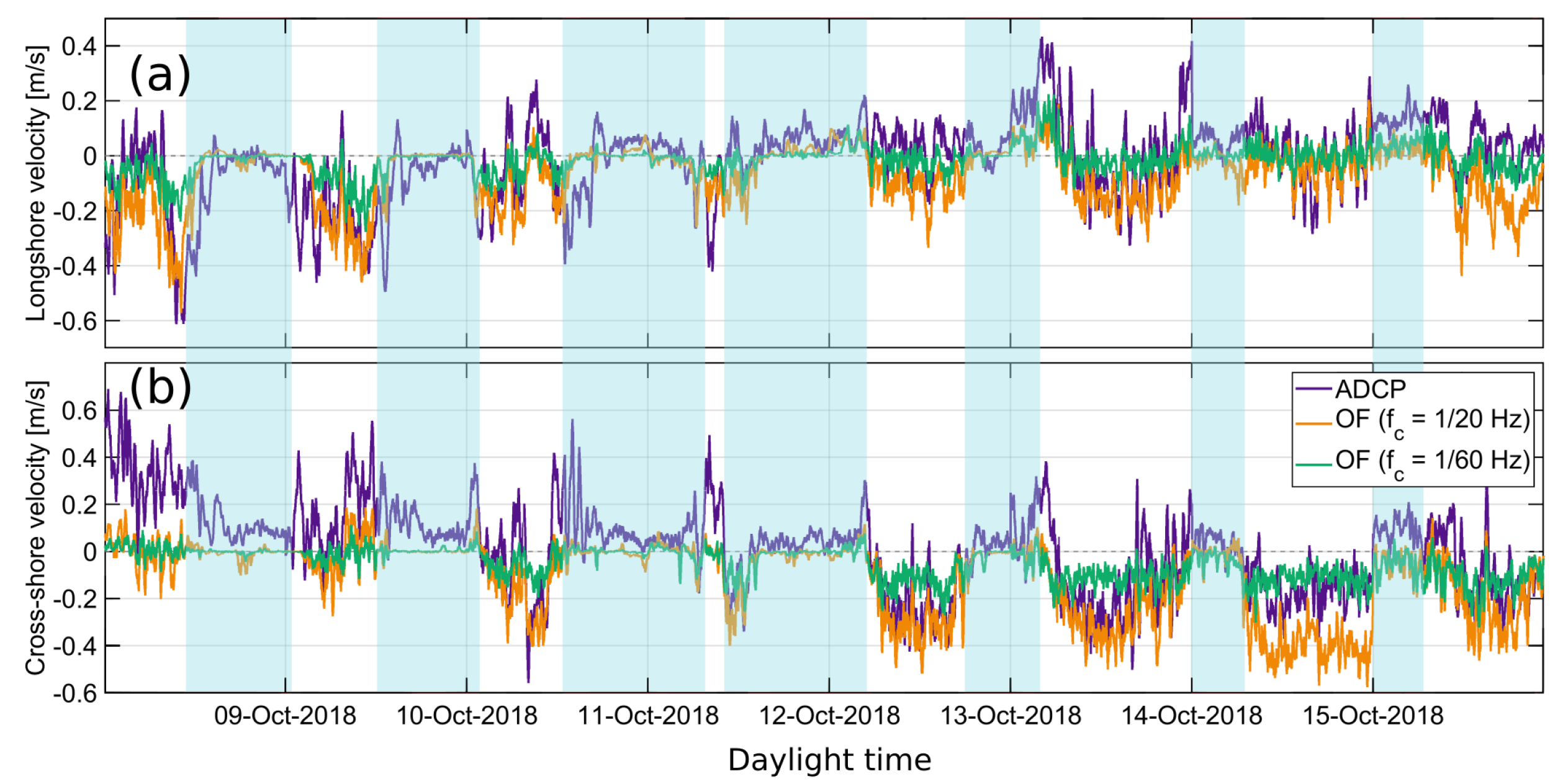
Figure 5 shows the 5-min time-averaged surface velocity components time series corresponding to 1-week of daylight measurements. For the longshore surface velocity component (Figure 5a), the optical flow derived-velocities recreate fairly well the slow fluctuations found in ADCP surface measurements. However, northward-directed currents (positive longshore velocity values) appear to be slightly underestimated. Regarding the cross-shore component (Figure 5b), onshore-directed currents overall match well between optical flow and ADCP, while offshore-directed velocities are less in agreement. This underestimation will be discussed in Section 6. In general, the optical flow velocities obtained using low-pass filtered images with $f_c=1/20$ Hz and $f_c=1/60$ Hz are similar in pattern. 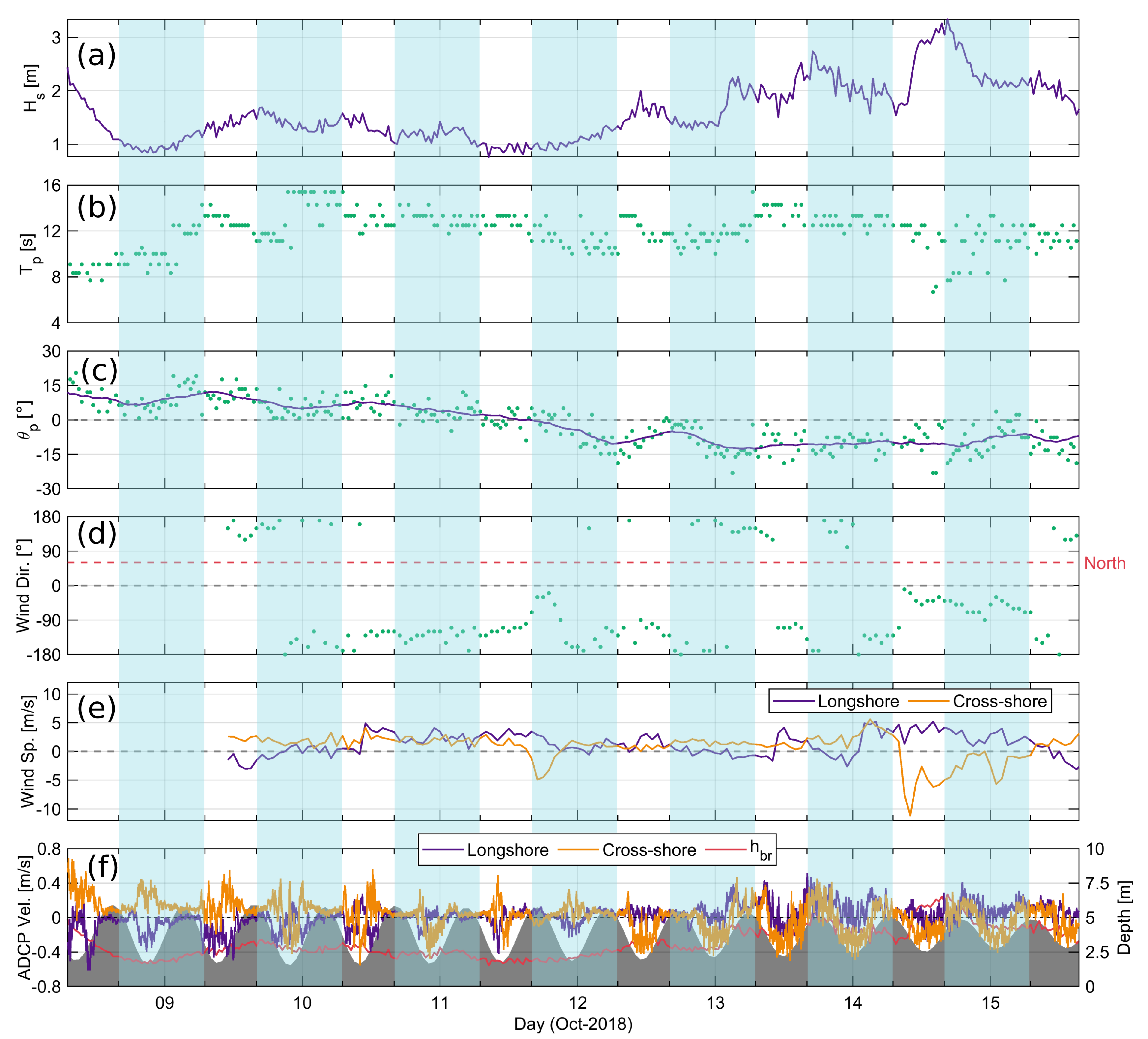However, OF ($f_c=1/60$ Hz) present a smaller amplitude (i.e., smaller velocities values) with respect to OF ($f_c=1/20$ Hz). It is important to note that near-zero optical flow values correspond to the time of high tide water elevation with $H_s<2$ m when no wave breaking was present over the reef and no foam was available for tracking close to the ADCP location (see Figure 2f; blue shaded regions in Figure 5).

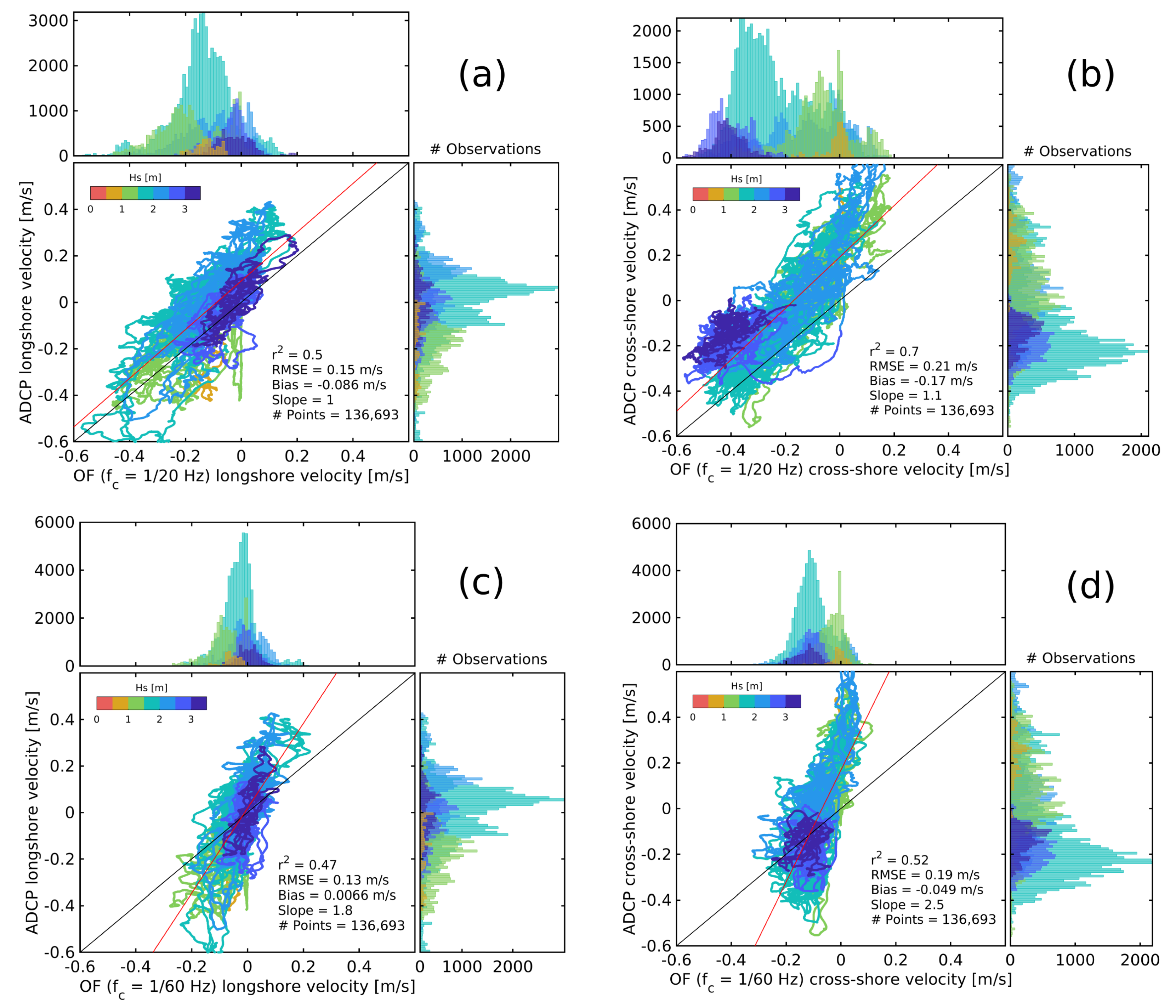
Figure 6 shows the 5-min time-averaged ADCP and optical flow surface velocity components of Figure 5 as a comparison under different ranges of significant wave height $H_s$. Surface velocities were grouped into seven $H_s$ bins of 0.5-m size. The corresponding statistics for each bin are summarized in

Table 2. Five minute time-averaged ADCP vs. optical flow surface velocity components from 8 to 15 October 2018 under different ranges of offshore significant wave height $H_s$ during low tide when the ADCP is located inside the surf zone. Optical flow velocities are computed from low-pass filtered images with $f_c=1/20$ Hz.

ADCP vs. OF (${\mathit{f}}_{\mathit{c}}=1/20$ Hz)	${\mathit{r}}^2$		RMSE [m/s]		Bias [m/s]		Slope		# Points (%)
thVelocity Component	thLong.	thCross.	thLong.	thCross.	thLong.	thCross.	thLong.	thCross.	thLong.	thCross.
${\mathit{H}}_{\mathbf{s}}<\mathbf{0}.\mathbf{5}$ m	-	-	-	-	-	-	-	-	0 (0%)
$\mathbf{0}.\mathbf{5}\le {\mathit{H}}_{\mathit{s}}<\mathbf{1}$ m	0.02	0.49	0.14	0.27	0.06	−0.26	0.45	1.52	3482 (3%)
$\mathbf{1}\le {\mathit{H}}_{\mathit{s}}<\mathbf{1}.\mathbf{5}$ m	0.31	0.69	0.12	0.19	−0.01	−0.16	0.69	1.38	26,879 (20%)
$\mathbf{1}.\mathbf{5}\le {\mathit{H}}_{\mathit{s}}<\mathbf{2}$ m	0.63	0.74	0.16	0.17	−0.13	−0.13	1.16	1.35	60,416 (44%)
$\mathbf{2}\le {\mathit{H}}_{\mathit{s}}<\mathbf{2}.\mathbf{5}$ m	0.67	0.68	0.16	0.24	−0.13	−0.20	1.28	1.24	25,920 (19%)
$\mathbf{2}.\mathbf{5}\le {\mathit{H}}_{\mathit{s}}<\mathbf{3}$ m	0.41	0.13	0.08	0.23	−0.01	−0.21	1.02	0.33	12,658 (9%)
${\mathit{H}}_{\mathit{s}}\ge \mathbf{3}$ m	0.69	0.59	0.07	0.27	−0.03	−0.27	1.29	0.59	7338 (5%)
${\mathit{H}}_{\mathit{s}}\ge \mathbf{0}$ m	0.50	0.70	0.15	0.21	−0.09	−0.17	1.00	1.13	136,693 (100%)

and

Table 3. Five minute time-averaged ADCP vs. optical flow surface velocity components from 8 to 15 October 2018 under different ranges of offshore significant wave height $H_s$ during low tide when the ADCP is located inside the surf zone. Optical flow velocities are computed from low-pass filtered images with $f_c=1/60$ Hz.

ADCP vs. OF (${\mathit{f}}_{\mathit{c}}=1/60$ Hz)	${\mathit{r}}^2$		RMSE [m/s]		Bias [m/s]		Slope		# Points (%)
Velocity Component	Long.	Cross.	Long.	Cross.	Long.	Cross.	Long.	Cross.	Long.	Cross.
${\mathit{H}}_{\mathit{s}}<\mathbf{0}.\mathbf{5}$ m	-	-	-	-	-	-	-	-	0 (0%)
$\mathbf{0}.\mathbf{5}\le {\mathit{H}}_{\mathit{s}}<\mathbf{1}$ m	0.07	0.38	0.18	0.27	0.13	−0.26	1.15	1.72	3482 (3%)
$\mathbf{1}\le {\mathit{H}}_{\mathit{s}}<\mathbf{1}.\mathbf{5}$ m	0.35	0.44	0.15	0.20	0.09	−0.12	1.37	2.93	26,879 (20%)
$\mathbf{1}.\mathbf{5}\le {\mathit{H}}_{\mathit{s}}<\mathbf{2}$ m	0.45	0.48	0.13	0.18	−0.02	0	1.73	2.35	60,416 (44%)
$\mathbf{2}\le {\mathit{H}}_{\mathit{s}}<\mathbf{2}.\mathbf{5}$ m	0.52	0.61	0.14	0.24	−0.05	−0.16	2.00	2.33	25,920 (19%)
$\mathbf{2}.\mathbf{5}\le {\mathit{H}}_{\mathit{s}}<\mathbf{3}$ m	0.06	0.01	0.10	0.11	0.03	0.08	0.72	0.20	12,658 (9%)
${\mathit{H}}_{\mathit{s}}\ge \mathbf{3}$ m	0.58	0.02	0.08	0.07	−0.01	0.02	2.17	0.21	7338 (5%)
${\mathit{H}}_{\mathit{s}}\ge \mathbf{0}$ m	0.47	0.52	0.13	0.19	0.01	−0.05	1.82	2.45	136,693 (100%)

and depicted with histograms of different colors in Figure 6. Around 80% of the velocity data is concentrated between 1 and 2.5 m of $H_s$. OF ($f_c=1/20$ Hz) and ADCP surface velocities within this range show a relatively good agreement ($r^2\approx 0.5$ and $\mathrm{RMSE}\approx 0.2$ m/s). However, the bias and the skewed bivariate histograms indicate a northward- and offshore-directed current underestimation that becomes more evident for $H_s>2.5$ m ($\mathrm{bias}\approx 0.2$ m/s).

Comparison between OF ($f_c=1/60$ Hz) and ADCP surface velocities shows a smaller bias and less dispersion of the data with respect to OF ($f_c=1/20$ Hz). Although $r^2$ suggests a similar linear agreement ($r^2\approx 0.5$), optical flow velocities are overall smeared as shown in the histograms of Figure 6c,d. This is also evidenced by the steeper values of the regression slope ($\mathrm{slope}>2$).

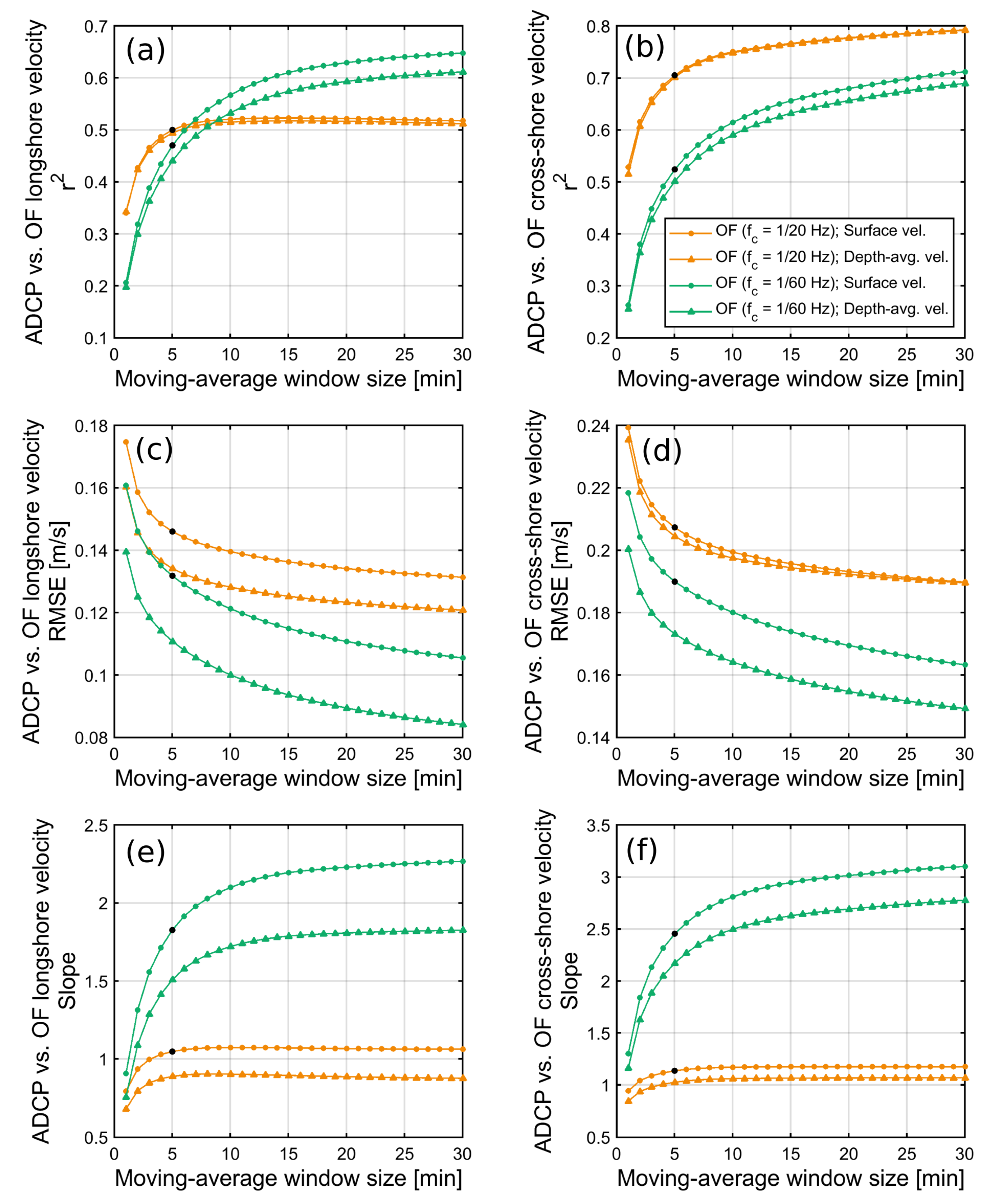
Figure 7 quantifies the agreement between optical flow surface velocity estimates and ADCP measurements. ADCP measurements consisted of surface velocities (average between ${\sigma }_{19}$, ${\sigma }_{20}$ and ${\sigma }_{21}$) and depth-averaged velocities (average of all $\sigma$-layers within the water column). The estimated and measured time series were moving-averaged and compared against different window size selections. Based only on $r^2$, the longshore surface velocity component (Figure 7a) is better reproduced by the optical flow when using low-pass filtered images with $f_c=1/60$ Hz as input. Comparison between OF ($f_c=1/60$ Hz) and ADCP surface velocities, for a window size larger than 10 min, show $r^2$ values ranging from 0.55 up to 0.65 with associated RMSE between 0.12 and 0.11 m/s. Similarly, OF ($f_c=1/60$ Hz) vs. ADCP depth-averaged velocities exhibit $r^2$ ranging from 0.5 up to 0.6 with lower RMSE between 0.10 and 0.08 m/s. A fair performance is still found when using low-pass filtered images with $f_c=1/20$ Hz. OF ($f_c=1/20$ Hz) vs. ADCP longshore velocity measurements (surface and depth-averaged velocities) show a consistent agreement ($r^2=0.5$) for any window size larger than 5 min, although RMSE values are relatively lower when compared against ADCP depth-averaged velocities (RMSE between 0.12 and 0.13) than with surface velocities (RMSE between 0.13 and 0.14). By contrast, ADCP cross-shore surface and depth-averaged velocities are better correlated with OF ($f_c=1/20$ Hz) than with OF ($f_c=1/60$ Hz) velocity estimates. For a window size larger than 5 min, $r^2$ values vary between 0.7–0.8 and 0.5–0.7, respectively (Figure 7b). OF ($f_c=1/20$ Hz) vs. ADCP cross-shore velocity RMSE decreases from 0.21 to 0.19 m/s as the window size increases from 5 to 30 min regardless if the optical flow estimates are compared against surface or depth-averaged ADCP velocities. On the other hand, as the window size increases from 5 to 30 min, OF ($f_c=1/60$ Hz) vs. ADCP cross-shore surface velocity RMSE decreases from 0.13 to 0.12 m/s and OF ($f_c=1/60$ Hz) vs. ADCP cross-shore depth-averaged velocity RMSE decreases from 0.11 to 0.08 m/s. In addition to $r^2$ and RMSE metrics, it is worth noting the values of the linear regression slope for both velocity components (Figure 7e,f). Slope values equal to one indicate a correct steepness for the one-to-one linear relationship between optical flow estimates and ADCP measurements. According to the regression slope, OF ($f_c=1/20$) velocity estimates indeed reproduce better the ADCP measurements for both velocity components with slope values around $1\pm 0.15$. Overall, as the window size is increased, high-frequency noise-related variability (i.e., RMSE) is reduced improving performance metrics (Figure 7c,d).

The bias has been intentionally omitted in Figure 7 as it poorly depends on the time-averaging window size. Regardless of the window size selection for the moving-average, the bias remain constant and correspond to the same values previously shown in Figure 6 and Table 2 and Table 3: OF ($f_c=1/20$ Hz) vs. ADCP longshore velocity bias $=-0.09$ m/s, OF ($f_c=1/20$ Hz) vs. ADCP cross-shore velocity bias $=-0.17$ m/s, OF ($f_c=1/60$ Hz) vs. ADCP longshore velocity bias $=0.01$ m/s and OF ($f_c=1/20$ Hz) vs. ADCP cross-shore velocity bias $=-0.05$ m/s. Moreover, the bias does not appear to change with ADCP surface or depth-averaged velocity measurements.

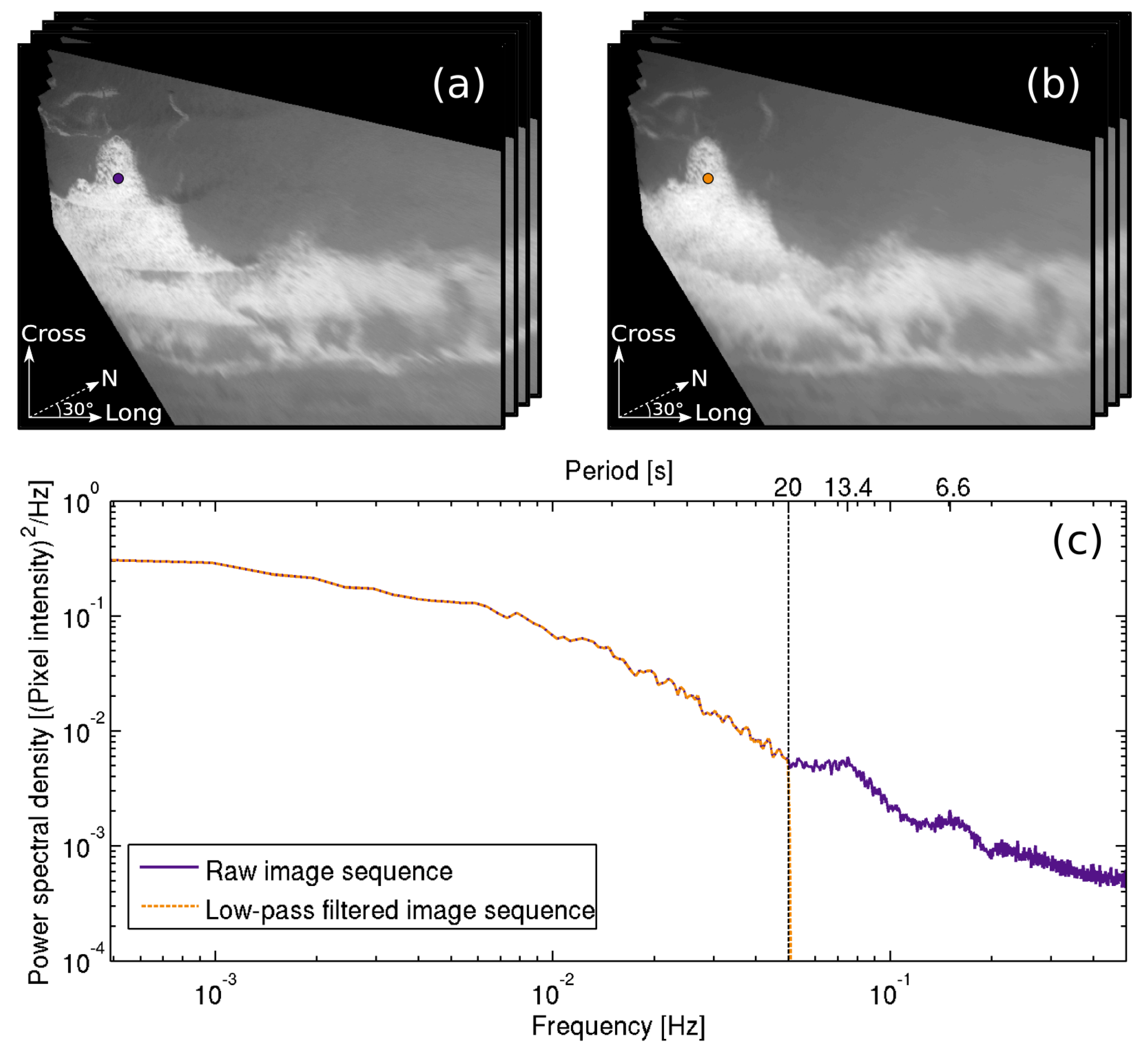
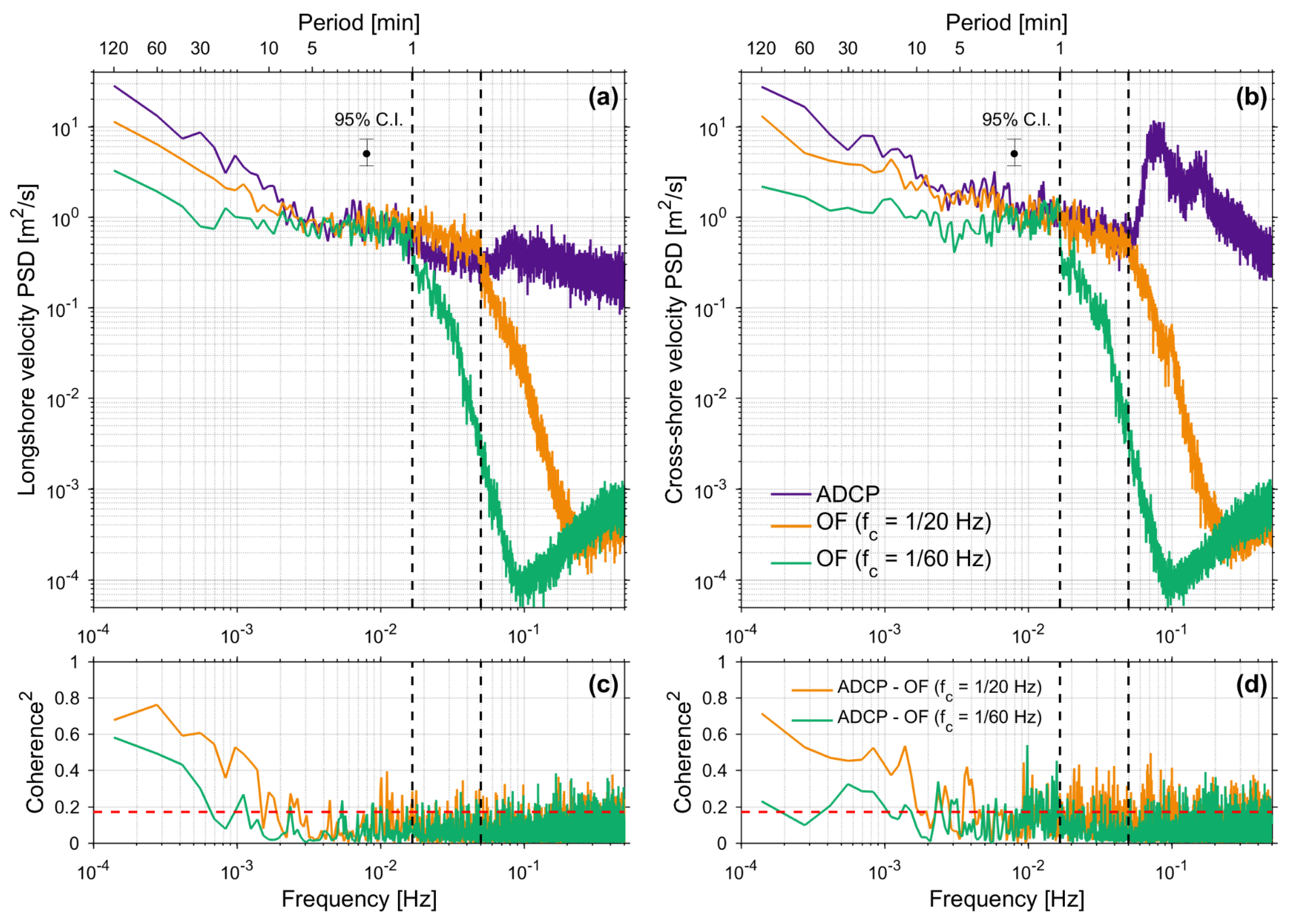
Figure 8 shows the surface velocity PSDs computed over the 17-averaged 2-h segments 1-week time series. The PSDs reveal a variety of signals present in both ADCP and optical flow time series (e.g., infragravity and VLF fluctuations). As expected, the velocity spectral energy associated with the sea-swell frequency band, previously removed from the image sequence, is subsequently attenuated for frequencies higher than the image low-pass filter cutoff-frequency ($f_c=1/20$ Hz and $f_c=1/60$ Hz; black dashed lines). The squared coherence is significant at the 95% confidence level in the infragravity frequency range (0.004–0.04 Hz) with values around 0.4 for the cross-shore velocity component. Nevertheless, the frequency region with the highest coherence (≈0.6) is associated with the VLF band (<0.004 Hz). Overall, the squared coherence shows a better agreement for OF ($f_c=1/20$ Hz) velocities. The low spectral energy found in OF ($f_c=1/60$ Hz) estimates is related to the low amplitude found in the surface velocity time series.

5.2. Drifter Deployments

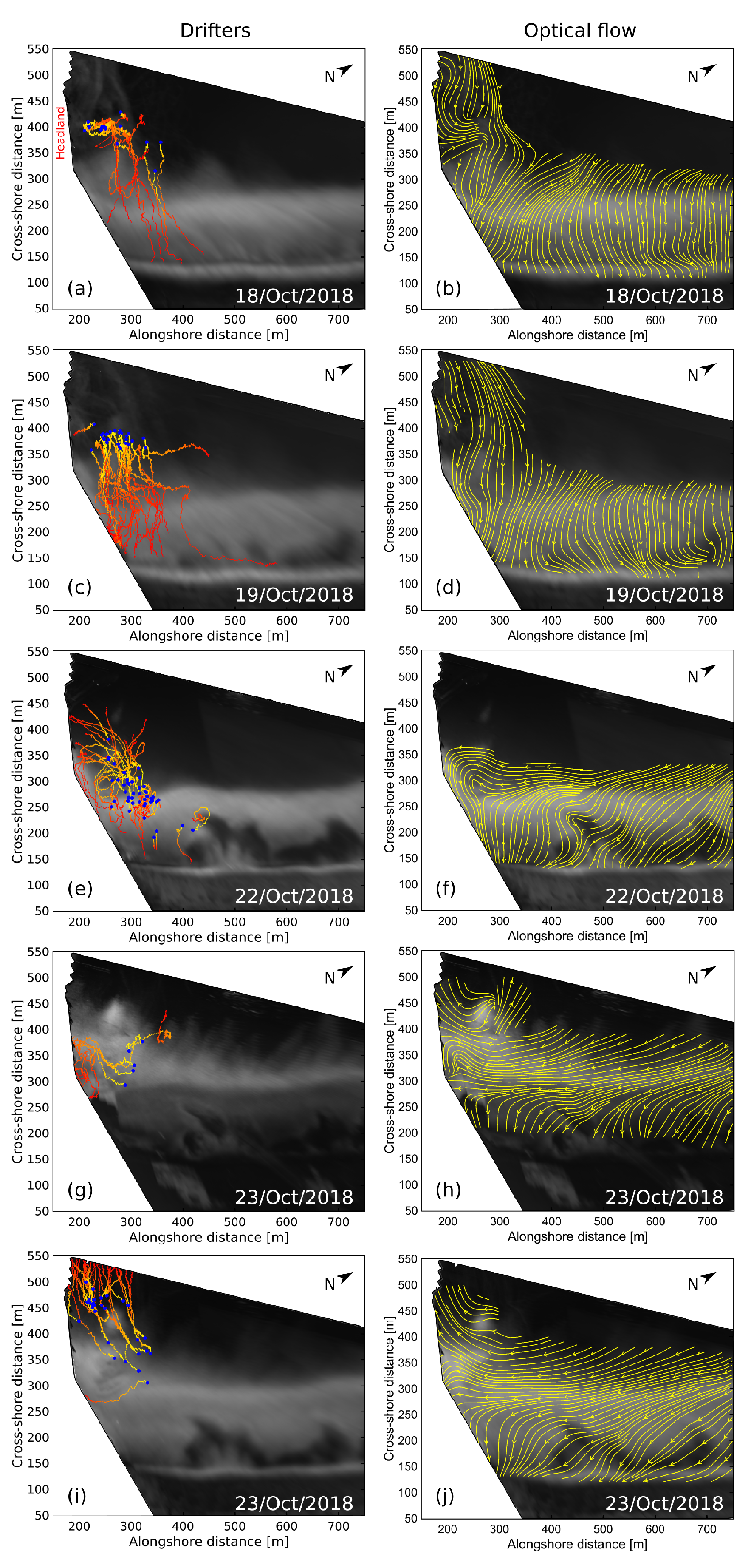
Figure 9 shows drifter tracks on 18, 19, 22 and 23 October 2018 along with corresponding optical flow stream plots under different field conditions (Table 1). The pixel intensity standard deviation image is also overlaid in each plot to highlight wave breaking spatial variability (e.g., surf zone and reef location) and foam availability during drifter deployment. Days corresponding to 18 and 19 October 2018 (Figure 9a–d) show evidence of primarily onshore-directed flows. Intermittent traces of foam along the headland made it possible to compute mean optical flow estimates outside the surf zone, although velocities in this region may not be reliable due to a lower number of observations [22]. This is the main reason why only qualitatively streamlines are shown to represent the mean surface flow.

More complex circulations are described by the drifters on 22 October 2018 (Figure 9e,f). The presence of a quasi-steady circulation cell at the location of the reef is displayed under a combination of moderate-energy and shore-normal incident waves ($H_s=1$ m; $T_p=11$ s; ${\theta }_p=0$°) around low tide. It is interesting to note the evolution of rip channels inside the surf zone which in turn influences the circulation. Nevertheless, optical flow estimation of the circulation patterns is consistent with the observed drifter tracks. Figure 9g presents the trajectories of the first set of drifters released around neap low tide on 23 October 2018, whereas Figure 9i shows the trajectories of the remaining drifters deployed during rising low tide. During low tide (Figure 9g,h), the wave-induced longshore current is deflected against the headland and affected by wave breaking across the reef resulting in a transient counter-clockwise circulation cell and a deflection rip. As the water level increases (Figure 9i,j), the reef exerts less control on rip dynamics allowing the dominant longshore current to completely deflect offshore resulting in a fully-developed deflection rip.

Movies were generated for the four days of drifter deployments and are provided as Supplementary Materials (Video S1, Video S2, Video S3 and Video S4). The movies contain the 2-min time-averaged optical flow velocity field overlapped with drifter trajectories. Overall, optical flow is able to recreate satisfactorily the main circulation patterns described by drifters trajectories reproducing smaller circulation structures with a great spatial resolution. Moreover, results are in agreement with previous studies describing the same events [40,44].

6. Discussion

6.1. Comparison to Other Optical Flow-Based Methods

In the context of coastal imagery, the shortcomings of the PIV approach and cross-correlation based methods, is that the estimated velocity field resolution is dependent on the size of the user-defined image segments (i.e., one displacement vector per image segment or window) being sparser than the input image resolution [21]. PIV is also prone to errors under conditions of insufficient surface texture, limiting it to spatially small areas [20]. On the other hand, the optical flow method is capable to provide a velocity vector at every pixel of the image. Despite the high potential of this technique, coastal applications are scarce [21,22,62] in contrast with PIV studies [19,20,27,28,29,30,31].

Table 4. Comparison of optical flow-based techniques previously reported in the literature for estimating nearshore surface currents under different field conditions at different sites.   

Optical Flow-Based Methods	Dérian and Almar (2017) [21]		Anderson et al. (2021) [22]		Present Study
	Typhoon		OpenCV		OpenOpticalFlow
${\mathit{f}}_{\mathit{s}}$ [Hz]	2		2		1
Image filtering approach	High-pass median filter		Moving-average		Low-pass filter
Study site	Grand Popo Beach, Benin		Duck, USA		PCA Beach, France
${\mathit{H}}_{\mathit{s}}$ range [m]	1.2–1.6		0.9–1.6		0.8–3.3
${\mathit{T}}_{\mathit{p}}$ range [s]	10–12		8–12		7–15
Water level range [m]	0.3 to 1.2		−0.14 to 0.90		1.5 to 5.9
Wind speed range [m/s]	-		3.3–7.4		0–12
In situ validation	ADV		Drifters		ADCP
Nearshore region	Swash/Surf zone		Surf zone		Surf zone
Velocity component	Longshore	Cross-shore	Longshore	Cross-shore	Longshore	Cross-shore
Number of points	8130	8130	>90	>90	136,992	136,992
${\mathit{r}}^{\mathbf{2}}$ range	0.13–0.29	0.05–0.58	-	-	0.35–0.51	0.51–0.80
RMSE range [m/s]	0.22–0.65	0.12–0.58	0.15	0.13	0.12–0.17	0.19–0.24

summarizes the performance of existing optical flow-based techniques previously reported in the literature [21,22] for estimating two-dimensional nearshore surface currents. The velocity outcomes provided by each method are compared with measurements from specific in situ instruments deployed under different field conditions at particular sites. The main difference between the three methods relies in the pre-processing of the images before the optical flow is applied. In Dérian and Almar [21] method, a two-dimensional spatial high-pass median filter is applied to each image in order to enhance the foam texture. While this filter improves the fine-scale foam patterns from large-scale structures such as propagating wave rollers, it does not remove the optical wave signal from the images. Their method has the potential to compute instantaneous (wave-by-wave fluctuations) surface velocities, however, the optical flow algorithm is also subject to track pixels propagating at wave celerity and disregard the actual flow. By contrast, Anderson et al. [22] and the present method filter the wave signal from the image sequence in order to track coherent foam patterns carried by the time-averaged flow, thus constraining the computed surface velocities below the sea-swell frequency band.

Dérian and Almar [21] compared shore-based image-derived surface velocities against near-bottom velocities collected from a single Acoustic Doppler Velocimeter (ADV) deployed within the swash zone. As the authors recognized, the comparison between optical flow estimates and instrument measurements was limited by their different location of the vertical profile. Despite drifter measurements acquired during the same field experiment were available [63,64], they were not considered in their analysis. On the other hand, Anderson et al. [22] compared optical flow derived-velocities against surf-zone drifters velocities using $15\times 15$ m spatial bins. As mentioned by Anderson et al. [22], drifters were often subject to surfing effects from localized wave-breaking such that they experienced motions at the scale of wave-by-wave fluctuations suggesting that in situ drifter might be unreliable tools for estimating mean currents at the scale of wave groups.

6.2. Low-Pass Filter Cutoff-Frequency Selection

The optical flow algorithm is very sensitive to the image input and the selection of the cutoff-frequency for the temporal low-pass filter can have a great impact on the final velocity estimates. OF ($f_c=1/60$ Hz) velocity estimates presented lower velocities and less spectral energy than ADCP measurements. For the temporal low-pass filter, using a cutoff-frequency of 1/60 Hz is equivalent to averaging images consecutively over 1 min. By proceeding with this selection, the dominant sea-swell band is evidently removed from the image sequence, however, all residual foam features become smeared and over-smoothed resulting in lower and underestimated velocity values (see histograms in Figure 6c,d). Furthermore, time-averaging these values can result in velocities close to zero with still a good linear correspondence to ADCP measurements with low RMSE and low bias. This can lead to a misinterpretation of good performance, as shown by the regression slope (Figure 6c,d and Figure 7e,f) and the damped velocity time series (Figure 5). By contrast, OF ($f_c=1/20$ Hz) velocity estimates demonstrate satisfactory agreement with surf-zone drifters tracks and ADCP measurements under relatively high-energy waves ($H_s<2.5$ m). Velocity RMSE of less than 0.25 m/s is a reasonably satisfactory result considering that the spatial resolution of the image grid is 1 m and the pixel footprint at the ADCP location is 0.6 m. On the other hand, the apparent bias and overall underestimation in offshore-directed currents (overestimation in onshore-directed currents) can be explained by other sources of error (see Section 6.4).

6.3. ADCP Measurements: Surface vs. Depth-Averaged Velocities

Directly comparing remote sensing products with in situ instruments is complicated. Optical flow estimates are representative of the motions occurring in the water surface layer, whereas, in the case of the ADCP, velocities corresponding to the upper region of the water column are usually removed to avoid possible errors associated with sidelobe interference, bubble injection, Stokes drift and wind contamination. Thus, it is difficult to evaluate “true” errors as velocities are compared from different locations of the vertical profile. However, for this particular study, the fact that $r^2$ and RMSE do not differ as much when compared against ADCP surface or depth-averaged velocities suggests that the vertical variability of the flow is nearly depth-uniform. Figure 10 illustrates three representative 2-h time-averaged velocity profiles in $\sigma$ coordinates. The velocity profiles were computed under different angles of wave incidence at low tide (around 2 and 3 m of water depth). The three configurations indicate shallow water flows with no significant vertical gradient, consistent with previous observations around the ADCP location [40,44]. These results show evidence of a nearly depth-uniform flow; however, for other locations inside the surf zone the visual surface layer might not always be representative of the entire water column. In case of strong vertical shear, the proposed ADCP transformation to $\sigma$ coordinates can be an alternative to derive velocities near the water surface consistent with video-derived estimates. However, caution must be exercised given the inherent limitations of the instrument when measuring close to the free surface.

6.4. Sources of Error

It should be noted that optical flow struggled to reproduce offshore-directed velocities at the ADCP location as revealed in the cross-shore velocity time series (Figure 5b) and the one-to-one comparison (Figure 6b). This can be mainly attributed to wave breaking. Although the frequency band corresponding to sea-swell waves is removed from the images, the source of foam, induced by wave breaking, appears as a blob that increases and spreads with time in the onshore direction following the filtered pre-existing wave front. Figure 11 illustrates the instantaneous circulation flow under wave breaking at two different instants separated by 7 s. In this representative example, ADCP velocities indicate a depth-uniform offshore-directed flow (as previously suggested). A close inspection of the optical flow velocity field near the ADCP location (Figure 11a,c) reveals instead a transient clockwise circulation cell which after 7 s (Figure 11b,d) is modified to be aligned with the incoming filtered wave front moving toward the shore. This effect is also observed with the isolated foam blob advancing around coordinates with alongshore distance = 410 m and cross-shore distance = 350 m (green polygon). However, this issue occurs in any region where strong wave breaking is present (e.g., reef and sandbar) and is also observed with low-pass filtered images with $f_c=1/60$ Hz. This suggests that the optical flow can erroneously track foam patches at the instant of their creation potentially masking true underlying velocities at those times. Therefore, a proper definition for the $f(x_1,x_2,I)$ term inside the physics-based optical flow equation (Equation (1)) is needed in order to account for specific foam properties such as source and dissipation rates, or alternatively, remove the velocity estimates associated with pixels that break in post-processing [22].

Surface velocity accuracy can also be limited by windage effects. Ideally, foam is expected to be advected only by the underlying currents, however, under high wind conditions, wind stress can induce surface currents that can advect the foam in a different direction than the desired surface/near-surface water flow. This could be probably the case during the relatively strong wind event on 14 October 2018, when wind speed reached up to 12 m/s. Other video-related sources of errors such as unwanted camera movement (e.g., produced by wind) [43,65], overlapping camera boundaries and tide dependent inaccuracies in geo-rectification [60] may also affect the performance of the optical flow-based technique and should be properly addressed before the optical flow method is applied.

6.5. Recommendations and Future Work

Optical flow is a powerful technique, however, certain factors and limitations must be considered in order to obtain satisfactory results. The first assumption, inherent to any optical flow algorithm, is that the pixel intensity between two consecutive frames should be nearly constant. Therefore, it is preferable to correct the scene illumination (e.g., by histogram equalization) before applying the optical flow method to increase accuracy. As described in Appendix A, we used a subroutine included in Liu [33] OpenOpticalFlow algorithm to correct the local illumination intensity changes between frames. Brightness variations can also be constrained to small changes if a coarse-to-fine scheme is used (see Appendix A) or if frames are sampled at a high rate (>1 Hz). However, this can have a direct impact on storage resources. An alternative to overcome this issue, as proposed by Anderson et al. [22], is to downsample the number of frames (e.g., by a factor of 5) once the dominant optical sea-swell wave signal is filtered from the image sequence, and then further apply the optical flow algorithm. Image temporal downsampling is possible after removing the wave clutter since the residual foam is smoothed in such a way that brightness variations between consecutive frames are kept low. However, filtering the optical signature from the images is a key step that must not be overlooked.

As shown in Figure 5, it is important to discard velocity values associated with pixels outside the surf zone or regions where no foam is present, otherwise, the optical flow algorithm will assign velocity values close to zero and underestimate the actual surface flow. For the ADCP pixel location we deduced the time when the instrument was inside the surf zone based on the water depth and kept only those corresponding velocity values. On the other hand, for the drifter experiments we removed all time-averaged velocities smaller than 0.02 m/s to ensure that the remaining velocities (streamlines) corresponded to regions where foam was present (e.g., surf zone). Future work should include a post-processing step, similar to the one proposed by Anderson et al. [22], to automatically identify and isolate foam regions based on a local pixel brightness variation threshold between frames in order to discard spurious velocities when there is limited texture on the water surface to track.

It should be noted that the intermittent wave breaking region where the ADCP was deployed was a particularly challenging location for the optical flow algorithm to produce accurate velocity estimations. Therefore, we propose that further research should be undertaken by mounting current profilers distributed at different locations within the surf zone to provide the optical flow algorithm the optimal conditions for a consistent comparison.

7. Conclusions

In this paper, we presented an alternative method to filter the dominant optical signal associated with sea-swell waves from an image sequence. Waves were removed from the image time series by applying a temporal Fourier low-pass filter to each pixel of the image. After image-wave-filtering, the residual foam left by wave breaking was used as a quasi-passive tracer and was assumed to be advected primarily by the underlying flow; wind conditions during the experiment were relatively weak with mean wind speed values around 3 m/s. Foam trajectories within the surf zone were tracked using Liu [33] open-source optical flow algorithm (“OpenOpticalFlow”) to derive wave-filtered surface velocities (comprising frequencies below 1/20 Hz and 1/60 Hz). We proposed an approach based on depth-normalization of the water profile ($\sigma$-layers) to retrieve surface velocities from ADCP measurements. A transformation of z to $\sigma$ coordinates ensures that the velocities derived from the ACDP are as consistent as possible with those estimated from the optical flow algorithm. Optical flow-derived velocities were compared with ADCP time-averaged surface and depth-averaged velocities. ADCP measurements displayed nearly depth-uniform time-averaged velocities. Time-averaged optical flow velocity estimates, using low-pass filtered images with $f_c=1/20$ Hz as input, showed to be in good agreement with ADCP measurements ($r^2=$ 0.5–0.8; $\mathrm{RMSE}=$ 0.12–0.24 m/s; bias $=-0.09$ to $-0.17$ m/s; $\mathrm{slope}=1\pm 0.15$; ${\mathrm{coherence}}^2=$ 0.4–0.6). By contrast, optical flow-derived velocities, using low-pass filtered images with $f_c=1/60$ Hz as input, were overall underestimated due to an over-smooth of the foam features. In any case, optical flow offshore-directed velocities were systematically underestimated. This outcome can be justified by waves breaking over the reef (i.e., ADCP location) that produce and advect foam persistently toward the shore. The onshore-directed motion of the foam, induced by wave breaking, can differ from the actual underlying flow and can inadvertently be captured by the optical flow algorithm. Despite this apparent limitation, optical flow was able to qualitatively reproduce with a good agreement the mean current circulation patterns described by drifter trajectories under different wave, tide and wind conditions. Among these patterns, a rip-circulation cell was captured as well as a prominent and persistent rip current flowing against the headland (deflection rip). Such findings highlight the ability to detect rip currents and associated circulations at different time-averaging scales providing new insights into surf-zone hydrodynamics and invaluable resources for beach safety strategy.