
Comparative Evaluation of Microwave L-Band VOD and Optical NDVI for Agriculture Drought Detection over Central Europe


1
Department of Civil Engineering, Middle East Technical University, Ankara 06800, Turkey
2
Department of Mechanical, Aerospace and Civil Engineering, University of Manchester, Manchester M13 9PL, UK
3
Sorbonne Université, UMR 7619 METIS, Case 105, 4 Place Jussieu, F-75005 Paris, France
*
Author to whom correspondence should be addressed.
Remote Sens. 2021, 13(7), 1251; https://doi.org/10.3390/rs13071251
Submission received: 9 February 2021
/
Revised: 19 March 2021
/
Accepted: 23 March 2021
/
Published: 25 March 2021
(This article belongs to the Special Issue Remote Sensing in Assessing Responses of Vegetation to Drought)
Abstract
:Agricultural droughts impose many economic and social losses on various communities. Most of the effective tools developed for agricultural drought assessment are based on vegetation indices (VIs). The aim of this study is to compare the response of two commonly used VIs to meteorological droughts—Moderate Resolution Imaging Spectroradiometer (MODIS) normalized difference vegetation index (NDVI) and Soil Moisture and Ocean Salinity (SMOS) vegetation optical depth (VOD). For this purpose, meteorological droughts are calculated by using a standardized precipitation index over more than 24,000 pixels at 0.25° × 0.25° spatial resolution located in central Europe. Then, to evaluate the capability of VIs in the detection of agricultural droughts, the average values of VIs anomalies during dry and wet periods obtained from meteorological droughts are statistically compared to each other. Additionally, to assess the response time of VIs to meteorological droughts, a time lag of one to six months is applied to the anomaly time series of VIs during their comparison. Results show that over 35% of the considered pixels NDVI, over 22% of VOD, and over 8% of both VIs anomalies have a significant response to drought events, while the significance level of these differences and the response time of VIs vary with different land use and climate conditions.
1. Introduction
Drought is one of the characteristics of the climate system that occurs at any time of the year without any warning and regardless of geographical boundaries or economic and political differences. Multiple studies have shown the far-reaching consequences of droughts and heatwaves on the social and economic conditions of the people in central Europe and other areas exposed to these conditions [1,2,3]. Therefore, understanding the characteristics of droughts and their interactions with different industries (e.g., agriculture, energy, commercials, and residences) is an essential step in providing effective measures for reducing their damages and for their proper management.
One of the drought mitigation ways is to evaluate and monitor it by using indicators that can determine its severity and persistence in a region. Most of the indicators used in drought monitoring studies are based on meteorological variables such as precipitation, temperature, or soil moisture. Among different meteorological drought indices, standardized precipitation index (SPI) has been used in many studies and has been shown to be effective in assessing meteorological drought conditions by using long-term precipitation patterns that are usually tied to streams, reservoirs, and groundwater levels [4,5].
With the advent of different remotely sensed observations related to vegetation cover and elongation of the length of their time series, it has become possible to use vegetation-based drought indices to assess the effects of drought events on vegetation cover and agriculture accurately. Different vegetation indices (VIs) have been developed based on the analysis of the reflective spectrum using a combination of infrared short-wave infrared (SWIR) and near-infrared (NIR) reflections. The principle behind VIs developed by land surface reflectances is mostly based on the absorption of visible red radiation by leaf chlorophyll and the reflection of NIR radiation by the leaf mesophilic layer in the structure of healthy plants, whereas this function works reversely in the case of diseased or water-stressed vegetation conditions. The normalized difference of NIR and SWIR radiances of Landsat Thematic Mapper (TM), called ND45 [6], normalized difference vegetation index (NDVI; [7]), and enhanced vegetation index (EVI; [8]) are examples of these indices that have been shown to be effective in the monitoring of vegetation water content, crop phenology, and patterns of crop production in different regions of the world [9,10,11,12]. Among different VIs, the NDVI is the most widely used VI due to its simplicity in transforming spectral bands, the easy procedure of its calculation, and its availability for a long time period [13,14,15,16].
On the other hand, other recently developed VIs such as soil moisture and ocean salinity (SMOS) vegetation optical depth (VOD) [17], a dimensionless variable that quantifies the canopy microwave emission attenuation by vegetation structure and water content, can also provide complete information on spatio–temporal variations of vegetation cover. In addition, VOD can solve many issues that cause impurities in the NDVI (e.g., inherent nonlinearity with plant measurements, sensitivity to canopy background brightness, and asymptotic signals over dense vegetation conditions). VOD, by its nature, differs from the optical measurement of vegetation covers and is linked mostly to the total crop productions through measurement of the amount of vegetation water in both woody and leafy components of all aboveground biomasses. One of the substantial advantages of VOD over NDVI is the availability of its retrievals during dark times of the day and cloudy days, which leads the VOD time series to have higher temporal resolution [18].
Multiple research studies have been conducted to assess the added value of VOD on the monitoring of drought [19,20,21], biomass evolution [22,23], and phenological monitoring [24,25,26]. There are also studies that analyzed its interaction with other existing VIs and its added value to them in reflecting plants water status [20], wildfire assessments [27], land surface phenology [28], vegetation dynamics [29,30], ecosystem management [31,32], drought monitoring [33,34], crop yield prediction [35], and monitoring of biomass and gross primary production [36,37].
A review of the above-mentioned studies reveals that in most cases, drought assessment studies use a single source VI (i.e., either optical or microwave-based indices) or use multi-source VIs in order to analyze the impact of specific drought events at country scales. Given that there are very limited studies using a combination of VIs (e.g., VOD and NDVI) for agricultural drought monitoring, and that the impact of using multi-source VIs on drought monitoring has yet not been explored widely, it seems there is still room for comprehensive clarification of the interactions between agricultural droughts and different VIs.
The goal of this study, hence, is to analyze comprehensively the response of two commonly used VIs derived from different sources (i.e., NDVI and VOD) to the drought events. To this end, a paired t-test is used to compare the average values of anomaly time series of both NDVI and VOD observations of 24,442 pixels over central Europe statistically during dry and wet periods that are determined by using a meteorological drought index (i.e., SPI). Moreover, to understand the effectiveness of VIs in capturing agricultural droughts better, the response time of VOD and NDVI VIs to the drought events (i.e., the time lag between emergence and termination of drought events from meteorological and VIs point of view), in addition to the significance level of the difference between their average values during dry and wet periods, are compared to each other according to the interactions of climate and land use conditions of pixels and relative performance of each index performing relatively better than the other over them.
2. Materials and Methods
2.1. Study Area
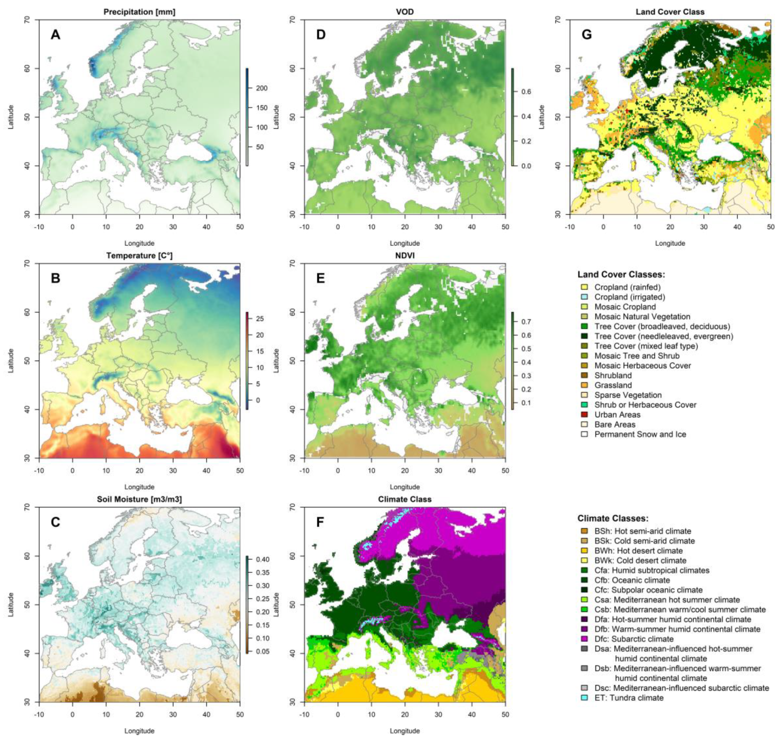
In order to compare the response of different VIs to meteorological drought events, in this study, the anomalies of NDVI and VOD VIs during dry and wet periods (derived by using SPI-12 time series) are statistically compared over 24,442 pixels located mainly in central Europe within the boundary of 10 W and 50 E longitudes and 30 N and 70 N latitudes. The selected boundary consists of 16 different land cover and 15 different climate classes that make it an appropriate region for investigating the interactions between different VIs and drought events on different climate and land use conditions. The spatial distribution of the long-term average of different climatic variables of precipitation [38], temperature [38], soil moisture [39,40,41], VOD [17,42,43], and NDVI [44], and the variety of climate [45] and land use [46] classes of studied area are presented in Figure 1. The detailed information about the time period, drought indices, and the steps that have been performed for the statistical comparison of VIs are presented below in Section 2.2 and Section 2.3.
The land cover and climate classes used in this study are retrieved by resampling the high-resolution ESA Climate Change Initiative (ESA-CCI) land cover map [46] and Köppen Climate Classification [45]. Given that the resampled land cover class at 0.25° × 0.25° resolution is composed of different high-resolution land cover classes with different probabilities, for all of the analyses that required the land cover classes of pixels, only those pixels were considered that consisted of a land cover class with more than 60% probability, in which the analysis of the response of VOD and NDVI VIs to meteorological droughts over those pixels that contain diverse high-resolution land cover classes are performed by using their average monthly precipitation, average temperature, and average NDVI variabilities. The application of this criterion significantly decreased the number of available pixels of different land cover classes. Here, only those land cover classes in which resampled products have more than 100 pixels over the study domain are considered in the analyses. Table 1 demonstrates the detailed information of the auxiliary datasets used in this study.
2.2. Drought Indices
2.2.1. Standardized Precipitation Index
Standardized Precipitation Index (SPI) can be calculated for any location based on the long-term precipitation data. The SPI index, proposed by McKee et al. (1993) [47], can be calculated by fitting long-term precipitation data into a probabilistic distribution and changing its shape to a normal distribution. The length of the precipitation time series and the nature of the probabilistic distributions play an important role in the calculation of SPI [48]. The ability to calculate the SPI drought index at different time scales (e.g., 1, 6, 12, and 24) can be considered as one of the advantages of this index [49]. In this study, among different SPI time scales, the SPI-12 is selected as the meteorological drought indicator due to its capability in accurate detection of drought durations [50]. The precipitation datasets used in the calculation of SPI-12 are obtained from ERA5 global reanalysis datasets [38] between years 1981 and 2019, while the gamma distribution is used to calculate the probability density function (PDF) of 12-month accumulated precipitation datasets. From here on SPI will be used to refer to SPI-12 for brevity. The PDF of accumulated precipitation records based on the gamma distribution can be calculated as follows:
where x is the accumulated precipitation amounts, α and β are the shape and scale parameters, respectively, and Γ(α) is the gamma cross function, which can be obtained as follows:
There are different methods available to estimate the shape and scale parameters of gamma distribution (i.e., α and β respectively). In this study, the estimation of gamma distribution parameters and calculation of SPI drought index values are performed by using SPEI package [51] in the R environment [52].
2.2.2. Normalized Difference Vegetation Index
The NDVI is a simple and practical index that has substantial sensitivity to vegetation dynamics. The NDVI values for the dense vegetation cover are close to one, while stones and bare soils are usually associated with values close to zero. The NDVI index can be calculated based on the following equation [53,54]:
where and are reflectance values at the near infra-red and the red band of the electromagnetic spectrum centered at 645 nm and 858 nm, respectively. Given that the seasonality component of variables often dominates the total variability of NDVI and is not associated with drought, the anomaly of NDVI time series is often used in drought monitoring and famine analysis. In this study, the NDVI anomalies are calculated by removing long-time monthly average values as follows:
where is the anomaly of NDVI for month i and year j, is the NDVI amount for the considered month i and year j, is the long-time average of NDVI values of month i, and is the long-term standard deviation of NDVI values of month i. The monthly NDVI values in this study are acquired from averaging Moderate Resolution Imaging Spectroradiometer (MODIS), MOD13C2, and MYD13C2 version 6 products [44] of the monthly scales between years 2010 and 2019, and 0.25° × 0.25° spatial resolution to be consistent with calculated SPI values and obtained VOD observations.
2.2.3. Vegetation Optical Depth
The VOD is a dimensionless variable that parametrizes the attenuation of the soil radiation by the vegetation canopy. The VOD observations, which are directly linked to the vegetation water content, are sensitive to the living biomass and woody content of canopy cover. There are multiple studies that recently showed the VOD derived from microwave observations can be used as an effective tool to monitor crops [18,55,56].
Currently, VOD is being retrieved from the C-, X-, Ku-, and L-band microwave observations of different radiometers since the year 1987 [56,57,58,59,60]. The radiometric nature of VOD retrievals, in comparison to other VIs that are usually derived from reflectances of visible and infra-red bands of optical sensors, has brought several advantages and drawbacks to this VI. Many studies have mentioned that VOD observations are less disposed to problems related to the presence of water vapor and clouds in the atmosphere [18]. On the other hand, the coarse resolution of radiometers and their sensitivity to the presence of radio frequency interference (RFI) and water bodies in the foot print of sensors are the main drawbacks of VOD observations that are revealed in different studies [61].
In this study, the monthly VOD time series are obtained at 0.25° × 0.25° resolution by monthly averaging the daily SMOS-IC L-band VOD retrievals (version 2 of the SMOS-IC dataset [17,42,43]) between years 2010 and 2019, at both ascending and descending orders. These daily VOD retrievals are initially filtered according to the RFI values (considering RFI probability threshold of 10% [62]) and the soil temperature using zero °C daily temperature values threshold of European Centre for Medium-Range Weather Forecasts (ECMWF) daily temperature values. Later, the filtered ascending and descending VOD observations are merged by using a simple averaging algorithm, and as a final step, a 30-day moving average smoothing filter is passed over the merged VOD time series to reduce the high-frequency noise of VOD retrievals.
The monthly VOD values are later converted to monthly anomalies by using the same approach used in the calculation of monthly NDVI anomalies as follows:
where is the anomaly of VOD for month i and year j, is the VOD amount for the considered month i and year j, is the long-time average of VOD values of month i and is the long-term standard deviation of VOD values of month i. For more detailed information about VOD observations and SMOS L-band retrieval algorithms used in the generation of daily VOD time series, refer to the study of Frappart et al. [18].
2.3. Statistical Analysis of Vegetation Cover Responses to Meteorological Droughts
In order to compare the response of vegetation cover to meteorological droughts, the average value of and during dry and wet periods are compared for their significance using a t-test. For this purpose, initially, the dry and wet periods are determined for the study area (with 0.25° × 0.25° resolution), using SPI time series and considering the criteria that a drought event should have, i.e., having at least a three-month duration and an SPI time series that falls below −1 once within a dry period [63].
As a second step, the anomaly time series of NDVI and VOD VIs (i.e., calculated using Equations (4) and (5) for NVDI and VOD, respectively) during dry and wet periods (defined using SPI time series) are extracted separately to create two paired NDVI and VOD anomalies for dry and wet conditions. Later, the average values of these paired values are compared between dry and wet periods using the t-test significance test. Here, the difference between the means of the VI during the dry and the wet periods are calculated so that greater differences between these two mean values imply greater sensitivity of the VI to the dry and the wet periods. Accordingly, this sensitivity of VI to drought and wetness is measured via p-value obtained from the t-test; lower p-values (i.e., probability of non-occurrence, or probability of finding significant difference just by chance while the null-hypothesis that there is no real difference is true) imply higher sensitivity and vice versa (i.e., higher p-values imply lower sensitivity). This analysis is performed pixel-wise through which a separate p-value is obtained for NDVI and VOD over each pixel.
For all pixels that VI values are available over them, the VI anomaly times series are shifted from zero to six months forward (with reference to SPI time series) to explore the time lag inherent between the drought (i.e., SPI) and the vegetation conditions (i.e., VIs). As a result of this comparison, the time lag that provides the least p-value is considered as the response time of VIs to drought events.
Later, p-values of NDVI and VOD over each pixel are compared. Accordingly, each pixel is assigned to one of four labels—VOD (VOD p-values are smaller than NDVI p-values), NDVI (NDVI p-values are smaller than VOD p-values), Both (if p-values of NDVI and VOD are the same, where p-values are rounded to have two significant decimals), and Non (p-values of NDVI and VOD are both not significant and higher than 0.05).
The spatial distribution of p-values is investigated so that the differences between the average p-values for each climate and land cover class are highlighted. Similarly, average p-values for the monthly average of total precipitation, temperature, soil moisture, NDVI, and VOD are also calculated. The interactions between climate and land use characteristics of identical pixels (pixels with the same VI class) and the significance level of difference between the average value of VOD and NDVI are explored to find the most suitable VI for monitoring agricultural drought events over different climate and land use conditions of the studied area. Here, it is worth noting that all of above-mentioned statistical analyses are performed using stats package in R environment [52].
3. Results
3.1. The Time Lag of Vegetation Cover Response to Meteorological Drought
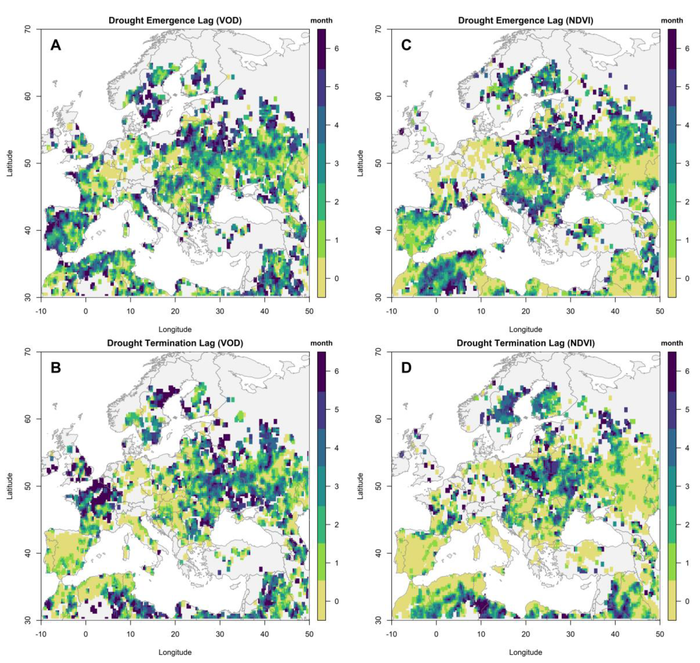
The time lag of vegetation cover response to meteorological drought is investigated by applying different lag times (one to six months) to the VIs anomalies and analyzing their corresponding significance level (i.e., non-occurrence probability) of differences in the average value of VOD and NDVI VIs anomalies during wet and dry periods. The spatial pattern of the time lag between the emergence of meteorological droughts and the appearance of their impacts on vegetation covers (i.e., Figure 2A,B) shows that in over 12% and 18% of the studied area from VOD and NDVI point of view, the vegetation covers respond to meteorological droughts within a month.
Moreover, a comparison of the response time of vegetation covers to the emergence and termination of meteorological droughts (Figure 2A,C for VOD and Figure 2B,D for NDVI) shows that, on average, there is a monotonic relationship between the response time of VOD and NDVI VIs to the meteorological drought events (i.e., when NDVI shows a higher lag time for the response of vegetation covers to meteorological droughts, VOD also shows a high lag time and vice versa); there are also regions in which the response time of VIs differ from each other (e.g., Iberian Peninsula and other regions around the Mediterranean Sea).
On the other hand, the comparison of the time lag between the termination of meteorological droughts and the disappearing of their impacts from vegetation cover shows that in over 11% and 18% of the studied area, the impacts of droughts on vegetation covers disappears without any lag time after termination of meteorological drought events, while on the contrary, there are some regions (14% and 12% percent of the studied area from VOD and NDVI point of view, respectively) in which the impacts of drought events remain for longer durations on vegetation cover (i.e., more than a month), after the termination of meteorological droughts (e.g., southern parts of the studied area).
3.2. The Significance Level of Vegetation Cover Response and Meteorological Drought Relationships
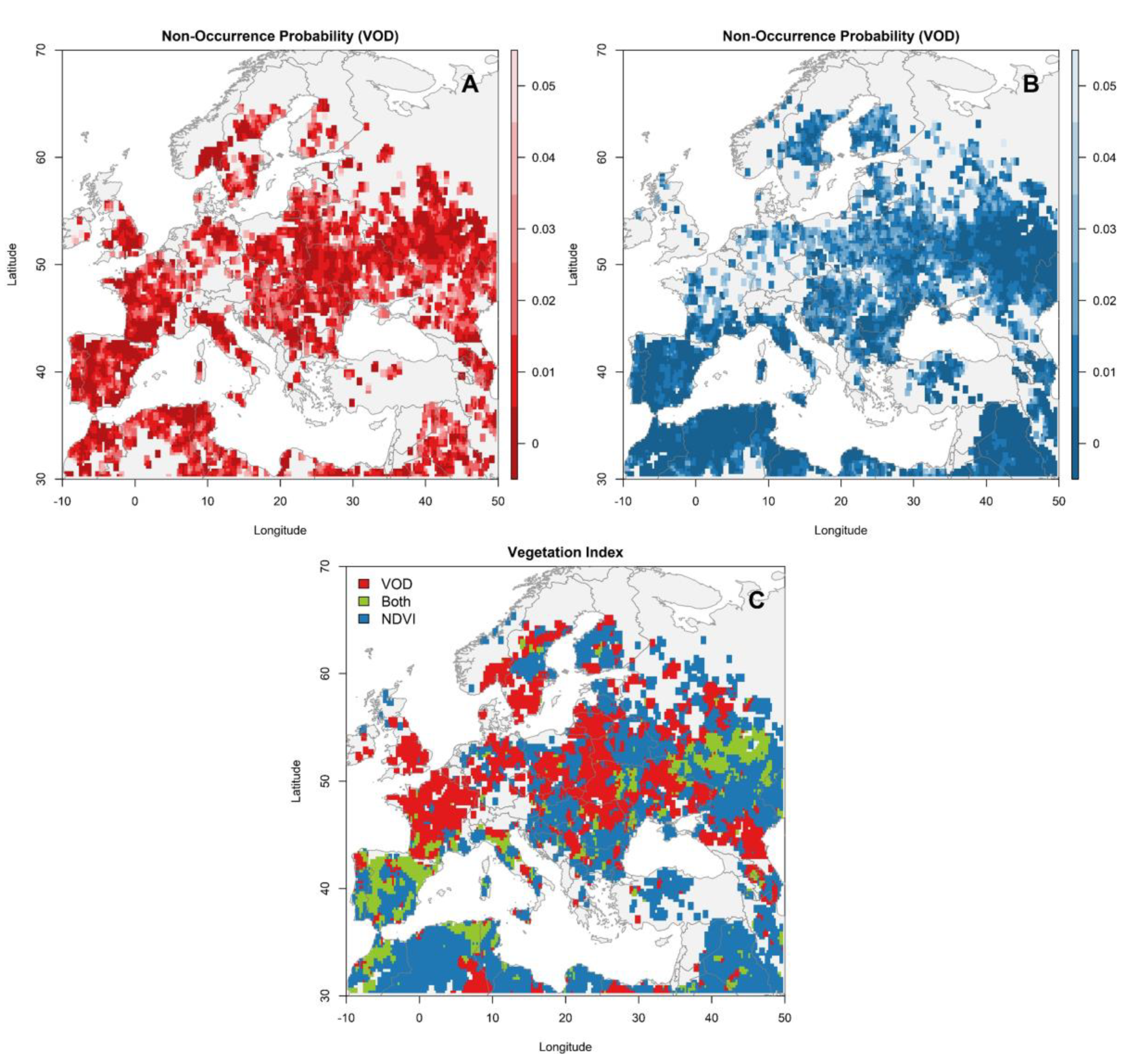
The significance level of vegetation cover response to the meteorological drought is explored through analyzing the non-occurrence probability of significant difference between the average value of anomalies of VIs (i.e., VOD and NDVI) during dry and wet periods, following the methodology introduced in Section 2.3. Figure 3 represents the spatial distribution of the assigned VI class (Figure 3C) to each pixel based on the significance level of their response to the meteorological droughts (Figure 3A,B).
The spatial variations of non-occurrence probability of significant difference in VIs anomalies during dry and wet periods show that VOD and NDVI have a significant response (with 0.05 non-occurrence probability) to the meteorological droughts in over 50% and 55% of the studied area, respectively, while there are also regions that none of VIs respond to meteorological droughts (e.g., regions with higher latitudes and colder temperature amounts).
The variation of the assigned VOD and NDVI classes to the pixels, based on their non-occurrence probabilities, as the most sensitive agricultural drought indicators (Figure 3C) shows that, except regions over higher latitudes with cold temperature and the regions that are excluded from the analysis due to their high RFI probability [64] (e.g., Turkey), most of the studied area is covered either with VOD, NDVI, or both of them. Overall, in over 22% of the studied area, the VOD anomalies, and in over 35% of the studied area, the NDVI anomalies respond with higher significant level (with lesser non-occurrence probability) to the meteorological drought events with respect to each other (e.g., France, and UK for VOD and Turkey and some other regions with Mediterranean climate for NDVI shown in Figure 3C), while there are regions (8% of the studied area) that both VOD and NDVI anomalies respond at the same significant level (with equal non-occurrence probability) to the meteorological drought events.
3.3. Impact of Climate and Land Use Variabilities on Agriculture Drought and Vegetation Indices Interactions
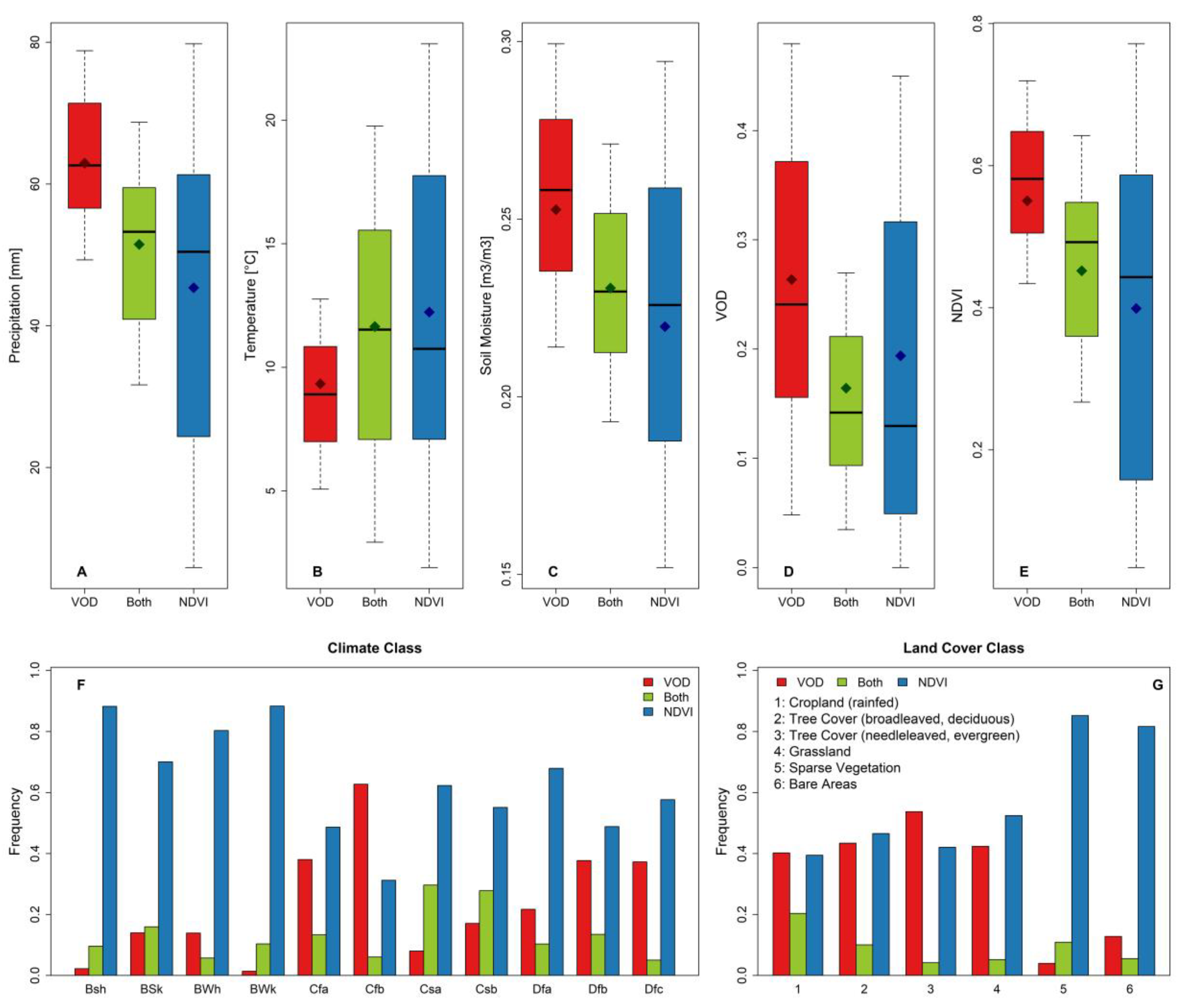
The impact of different climate and land use conditions on the significance level of vegetation cover response to the meteorological droughts are investigated through analyzing of spatial variation of different climate and land-use variables (i.e., total monthly precipitation, average temperature, average soil moisture, average VOD, and average NDVI) over pixels in which anomalies of VOD and NDVI VIs exposed to have significantly different average values during dry and wet periods (Figure 4A–E). Moreover, the coverage percentage of the pixels with an identical climate or land use class by each VI (either VOD, NDVI, or both) is calculated to determine the performance of each VI in the identification of agricultural droughts over different climate and land use classes (Figure 4F,G).
Based on the spatial variation of climatic variables over the pixels where anomalies of VOD and NDVI VIs exposed to have different average values during dry and wet periods, those pixels in which NDVI is selected as agricultural drought indicator over them, have a broader range of climate and land-use variability in comparison to those pixels that are assigned with VOD label. For example, 50% of the total monthly precipitation amounts (between 0.25 and 0.75 quantiles) varies between 56 and 71 mm per month over regions that VOD performs better than NDVI, while the 50% variation of total monthly precipitation over the regions that NDVI performs better than VOD is changing between 24 and 61 mm per month (Figure 4A). This less variability is also visible when the 50% of average NDVI values of the pixels are considered (0.50 to 0.64 variation for VOD vs. 0.15 to 0.58 variation for NDVI in Figure 4E), which implies that the agricultural drought can be captured through VOD over specific climate and land use conditions, while NDVI can be used as agricultural drought indicator in different climate and land use conditions.
Moreover, based on the same analysis, VOD can detect agricultural droughts over pixels with higher precipitation (Figure 4A) in comparison to NDVI (i.e., the mean value of monthly precipitation over pixels in which VOD and NDVI VIs have significant average values during dry and wet periods are 62 and 45 mm per month, respectively). The same is also visible over the variation of soil moisture (Figure 4C), where VOD can capture agricultural droughts over pixels with lesser average soil moisture (with average soil moisture of 25%), in comparison to NDVI that can capture agricultural droughts better over pixels with average soil moisture of 21%.
Moreover, the variation of average VOD and NDVI of pixels in which anomalies of VOD and NDVI VIs perform better than each other in capturing agricultural droughts (Figure 4D,E, respectively) show that VOD can capture agricultural droughts better than NDVI over denser vegetated regions (i.e., the average NDVI values over the regions that VOD performs better than NDVI is 0.55, while the average NDVI value of the pixels that NDVI performs better is 0.39). This is also visible over VOD variations in which the average VOD values for the pixels that VOD performs better than NDVI in the determination of agricultural drought are 0.26, while the average VOD value of pixels that NDVI performs better than VOD in agricultural drought determination is 0.19, supporting previous studies that also shown the reduced saturation of VOD over the regions with higher vegetation contents (e.g., forests) [22,37].
On the other hand, the variation of the average temperature values of pixels with assigned VIs of VOD or NDVI demonstrates that VOD performs better than NDVI over the colder regions (i.e., regions with an average temperature of 9 °C) in capturing agricultural droughts, while NDVI performs better in slightly warmer pixels with the average temperature value of 12 °C. Although the temperature variation is not that much among the pixels with different VI assigned to them, the climate type variation of pixels with assigned VIs can also be seen from the coverage percentages of different VIs over the pixels with different identical climate and land use classes (Figure 4F); where the majority of pixels with hot climate classes (i.e., Bsh, Bsk, BWh, and Bwk) are covered by NDVI with the average percentage of 82%, and pixels over regions with Oceanic climate class (i.e., Cfb), are mostly (more than 60%) covered by VOD VI (i.e., the coverage percentages in the sixth column of Figure 4F).
Likewise, the performance of VOD and NDVI VIs in capturing agricultural droughts over different land-use classes (Figure 4G), show that the VOD is most effective in capturing agricultural droughts over croplands and forested areas (particularly over dense forests that are mainly covered by evergreen trees). On the other hand, the coverage percentages of NDVI over different land use classes, show that over bare lands and those regions with sparse vegetation covers (e.g., Maghreb, and southern Mediterranean countries in Africa) NDVI is the dominant VI with 82% and 85% coverage percentage, respectively.
4. Discussion
The pixel-wise comparison of regions that VOD and NDVI or both of them responded to drought events significantly demonstrates that with the combined use of VOD and NDVI VIs, it is possible to monitor agricultural droughts over 64% of the pixels. On the other hand, the same analysis shows that while over the 42% of pixels, both VOD and NDVI VIs provide a significant response varying at significance levels (p-value varying between zero and 0.05), over 8% of the pixels, only VOD, and over 14% of the pixels, only NDVI provides a significant response to drought events. These results imply the added value of VIs derived from different sources to each other and the contribution of the proposed approach in the expansion of areas that agricultural droughts can be monitored over them. In addition, it is worth noting that the analyses associated with the identification of pixels for which NDVI or VOD perform better than each other over them are performed at 0.25° × 0.25° spatial resolution, where VOD anomalies, despite their coarse resolution, provide reasonable solutions compared to monthly NDVI values that are obtained by averaging NDVI values at 250-m resolution.
The analysis of the spatial distribution of time lag between the emergence of meteorological drought and response of vegetation covers to it shows that the late response times (i.e., time lags more than two months) are mostly associated with tree cover land use types (particularly forests consisting evergreen trees), while there is also a positive correlation between the response time of vegetated covers to the agricultural droughts and the density of their green leaves. The late response time of trees to drought events is mostly because of the root system of trees that allows them to have access to more stable water resources and meanwhile supports them by nutrient uptakes during drought events [65,66]. These findings are consistent with previous studies that showed similar results in different case studies that vegetation covers of forests may respond to meteorological droughts with a time lag and also remain for a longer period after their termination from a meteorological point of view [67,68].
The variation of climate variables such as precipitation over those pixels with identical VI as agricultural drought indicator (Figure 4) also demonstrates that VOD VI is mostly superior over wet regions and NDVI VI over dry regions with bare land or sparse vegetation covers. The reason for this might arise from the fact that over wet regions with a high amount of average monthly precipitation rates, the number of cloudy days is more than in other regions. The presence of clouds in the atmosphere does not allow optical sensors to retrieve observations ideally, while the nature of VOD observation and its radar-based retrieval method, help this VI to measure vegetation attenuation during cloudy days as well.
On the other hand, the comparison of behaviors of VOD and NDVI VIs in terms of their response time to meteorological droughts show that although there is a monotonic relationship between their response time, on average, over those pixels where NDVI responses to meteorological drought with five or six months of lag time, VOD responses with shorter lag time (i.e., four months), which implies the superiority of VOD VI in capturing drought impacts on vegetation covers of regions with higher leaf area and photosynthesis activity because the continuous development of photosynthesis activity over these regions leads NDVI values to remain in higher amounts even when the vegetation water content decreases as a result of drought events [26,69]. These results also demonstrate the added value of VOD to NDVI in earlier detection of damaged vegetated areas by agricultural droughts and the potential of the proposed approach in the development of early drought warning systems.
Moreover, the variation of monthly average NDVI values of pixels with identical vegetation (VOD or NDVI) supports this idea that NDVI is more effective in capturing agricultural droughts over regions with lower monthly average NDVI values (e.g., bare lands and sparsely vegetated areas), while VOD can be useful in agricultural drought identification over regions with higher monthly average NDVI values (Figure 4E). This can be related to the challenges linked with the saturation of NDVI at densely vegetated conditions where NDVI does not respond to leaf area expansion and remain the same at different vegetation condition levels. This implies that the VOD can significantly contribute to drought monitoring over dense vegetation covers such as evergreen forests and also reducing climate extreme risks through its advantage in earlier response time to meteorological droughts in comparison to NDVI (i.e., the response time difference of NDVI and VOD illustrated Section 3.1 and in Figure 3). Finally, the results related to the performances of VIs over croplands show that, as expected, both NDVI and VOD do not respond to meteorological drought over irrigated lands. However, results related to the coverage percentage of pixels with rainfed cropland covers show that both VOD and NDVI VIs anomalies have significantly different average values during dry and wet periods over them, and hence, they can be used as a handy tool in crop yield estimation studies. These findings support prior studies that combined optical and microwave VIs observations through machine learning algorithms and used their lag as an indicator for crop yield information [35] and suggest the existence of opportunity in better estimation of crop yields and improved monitoring of biomass accumulation at farm scale through synergistic use of high-resolution radar Sentinel-1 and optical Sentinel-2 imagery observations [35,56].
5. Conclusions
This study aimed to analyze the response of two VIs of MODIS NDVI and SMOS VOD to meteorological droughts through statistical comparison of average values of their anomalies during dry and wet periods derived by using a meteorological drought index (SPI-12). To this end, the response time of NDVI and VOD VIs to meteorological droughts (i.e., the time lag between emergence and termination of droughts after meteorological presence) are compared to each other.
Based on the significance level of the differences between the average values of NDVI and VOD anomalies during dry and wet periods, for each pixel (at 0.25° × 0.25° resolution) an index (either NDVI, VOD, or both) is assigned as an agricultural drought indicator. Moreover, to inspect the impact of land cover and climate conditions on the performance of VIs in capturing agricultural drought index, the climate and land use characteristics of pixels with identical assigned VI are analyzed and their interactions are explored.
Overall, results suggest that NDVI and VOD VIs can detect agricultural droughts as a response to meteorological droughts with different significance levels based on land use and climate cover conditions. While over pixels located in tree-covered areas (e.g., forests) VOD is more sensitive to meteorological droughts, over areas with sparse vegetation or bare land covers, NDVI can capture agricultural droughts more significantly. Moreover, results related to the spatial patterns of response times of VOD and NDVI anomalies demonstrate that although the NDVI and VOD VIs have very similar response time patterns, there are some regions where VOD and NDVI VIs may respond earlier than each other to meteorological droughts (e.g., the relative earlier response of VOD and NDVI anomalies to meteorological droughts over forests and bare lands, respectively).
Based on these findings, it can be concluded that there is not a single VI that can significantly capture agricultural droughts over all different land use covers and climate class conditions, and hence, it is necessary to monitor agricultural droughts over different land use covers and climate classes with a specific VI or combination of them to develop early warning systems for agricultural droughts and avoid losses associated with them.
Author Contributions
Conceptualization, M.H.A., A.A.-Y., and M.T.Y.; methodology, M.H.A., A.A.-Y., and M.T.Y.; formal analysis, M.H.A.; investigation, M.H.A., A.A.-Y., and M.T.Y.; data curation, M.H.A., A.A.-Y., and M.T.Y.; writing—original draft preparation, M.H.A.; writing—review and editing, M.H.A., A.A.-Y., and M.T.Y.; visualization, M.H.A. All authors have read and agreed to the published version of the manuscript.
Funding
This research received no external funding.
Institutional Review Board Statement
Not applicable.
Informed Consent Statement
Not applicable.
Data Availability Statement
The SMOS IC VOD datasets are obtained from “https://ib.remote-sensing.inrae.fr/” (accessed on 25 March 2021). The ERA5 global reanalysis datasets are obtained from doi:10.1002/qj.3803 (accessed on 25 March 2021). The Köppen climate class classification is obtained from “http://koeppen-geiger.vu-wien.ac.at/” (accessed on 26 March 2021.The ESA-CCI land cover classification is obtained from “https://www.esa-landcover-cci.org/” (accessed on 25 March 2021). The ESA-CCI soil moisture datasets are obtained from https://esa-soilmoisture-cci.org/ (accessed on 25 March 2021). The NDVI datasets are obtained from “lpdaac.usgs.gov” (accessed on 25 March 2021).
Acknowledgments
Authors thank INRAE BORDEAUX for SMOS IC VOD product (“https://ib.remote-sensing.inrae.fr/”; accessed on 25 March 2021), ECMWF for the ERA5 datasets, ESA Climate Change Initiative consortium for the ESA-CCI products, and the Land Processes Distributed Active Archive Center (LP DAAC; “lpdaac.usgs.gov”; accessed on 25 March 2021) for providing access to the MODIS data used in this study.
Conflicts of Interest
The authors declare no conflict of interest.
References
- Bezak, N.; Mikoš, M. Changes in the Compound Drought and Extreme Heat Occurrence in the 1961–2018 Period at the European Scale. Water 2020, 12, 3543. [Google Scholar] [CrossRef]
- Schuldt, B.; Buras, A.; Arend, M.; Vitasse, Y.; Beierkuhnlein, C.; Damm, A.; Gharun, M.; Grams, T.E.E.; Hauck, M.; Hajek, P.; et al. A first assessment of the impact of the extreme 2018 summer drought on Central European forests. Basic Appl. Ecol. 2020. [Google Scholar] [CrossRef]
- Ahmed, K.R.; Paul-Limoges, E.; Rascher, U.; Damm, A. A First Assessment of the 2018 European Drought Impact on Ecosystem Evapotranspiration. Remote Sens. 2021, 13, 16. [Google Scholar] [CrossRef]
- Mishra, A.K.; Singh, V.P. A review of drought concepts. J. Hydrol. 2010, 391, 202–216. [Google Scholar] [CrossRef]
- Zargar, A.; Sadiq, R.; Naser, B.; Khan, F.I. A review of drought indices. Environ. Rev. 2011, 19, 333–349. [Google Scholar] [CrossRef]
- Kimes, D.S.; Markham, B.L.; Tucker, C.J.; McMurtrey, J.E., III. Temporal relationships between spectral response and agronomic variables of a corn canopy. Remote Sens. Environ. 1981, 11, 401–411. [Google Scholar] [CrossRef]
- Rouse, J.W.; Haas, R.H.; Schell, J.A.; Deering, D.W. Monitoring vegetation systems in the Great Plains with ERTS. NASA Spec. Publ. 1974, 351, 309. [Google Scholar]
- Matsushita, B.; Yang, W.; Chen, J.; Onda, Y.; Qiu, G. Sensitivity of the enhanced vegetation index (EVI) and normalized difference vegetation index (NDVI) to topographic effects: A case study in high-density cypress forest. Sensors 2007, 7, 2636–2651. [Google Scholar] [CrossRef] [Green Version]
- Kath, J.; Le Brocque, A.F.; Reardon-Smith, K.; Apan, A. Remotely sensed agricultural grassland productivity responses to land use and hydro-climatic drivers under extreme drought and rainfall. Agric. For. Meteorol. 2019, 268, 11–22. [Google Scholar] [CrossRef]
- Nanzad, L.; Zhang, J.; Tuvdendorj, B.; Nabil, M.; Zhang, S.; Bai, Y. NDVI anomaly for drought monitoring and its correlation with climate factors over Mongolia from 2000 to 2016. J. Arid Environ. 2019, 164, 69–77. [Google Scholar] [CrossRef]
- Zhou, X.; Yamaguchi, Y.; Arjasakusuma, S. Distinguishing the vegetation dynamics induced by anthropogenic factors using vegetation optical depth and AVHRR NDVI: A cross-border study on the Mongolian Plateau. Sci. Total Environ. 2018, 616, 730–743. [Google Scholar] [CrossRef]
- Afshar, M.H.; Foster, T.; Higginbottom, T.P.; Parkes, B.; Hufkens, K.; Mansabdar, S.; Ceballos, F.; Kramer, B. Improving the Performance of Index Insurance Using Crop Models and Phenological Monitoring. Remote Sens. 2021, 13, 924. [Google Scholar] [CrossRef]
- Marco-Dos Santos, G.; Melendez-Pastor, I.; Navarro-Pedreño, J.; Koch, M. Assessing Water Availability in Mediterranean Regions Affected by Water Conflicts through MODIS Data Time Series Analysis. Remote Sens. 2019, 11, 1355. [Google Scholar] [CrossRef] [Green Version]
- Kim, H.W.; Kim, J.-H.; Li, W.; Yang, P.; Cao, Y. Exploring the impact of green space health on runoff reduction using NDVI. Urban For. Urban Green. 2017, 28, 81–87. [Google Scholar] [CrossRef]
- Natsagdorj, E.; Renchin, T.; De Maeyer, P.; Darkhijav, B. Spatial Distribution of Soil Moisture in Mongolia Using SMAP and MODIS Satellite Data: A Time Series Model (2010–2025). Remote Sens. 2021, 13, 347. [Google Scholar] [CrossRef]
- Bulut, B.; Yılmaz, M.T.; Afshar, M.H.; Şorman, A.Ü.; Yücel, İ.; Cosh, M.H.; Şimşek, O. Evaluation of Remotely-Sensed and Model-Based Soil Moisture Products According to Different Soil Type, Vegetation Cover and Climate Regime Using Station-Based Observations over Turkey. Remote Sens. 2019, 11, 1875. [Google Scholar] [CrossRef] [Green Version]
- Wigneron, J.-P.; Li, X.; Frappart, F.; Fan, L.; Al-Yaari, A.; De Lannoy, G.; Liu, X.; Wang, M.; Le Masson, E.; Moisy, C. SMOS-IC data record of soil moisture and L-VOD: Historical development, applications and perspectives. Remote Sens. Environ. 2021, 254, 112238. [Google Scholar] [CrossRef]
- Frappart, F.; Wigneron, J.P.; Li, X.; Liu, X.; Al-Yaari, A.; Fan, L.; Wang, M.; Moisy, C.; Le Masson, E.; Lafkih, Z.A.; et al. Global monitoring of the vegetation dynamics from the vegetation optical depth (VOD): A review. Remote Sens. 2020, 12, 2915. [Google Scholar] [CrossRef]
- Rao, K.; Anderegg, W.R.L.; Sala, A.; Martínez-Vilalta, J.; Konings, A.G. Satellite-based vegetation optical depth as an indicator of drought-driven tree mortality. Remote Sens. Environ. 2019, 227, 125–136. [Google Scholar] [CrossRef] [Green Version]
- Zhang, Y.; Zhou, S.; Gentine, P.; Xiao, X. Can vegetation optical depth reflect changes in leaf water potential during soil moisture dry-down events? Remote Sens. Environ. 2019, 234, 111451. [Google Scholar] [CrossRef]
- Al-Yaari, A.; Wigneron, J.P.; Ciais, P.; Reichstein, M.; Ballantyne, A.; Ogée, J.; Ducharne, A.; Swenson, J.J.; Frappart, F.; Fan, L.; et al. Asymmetric responses of ecosystem productivity to rainfall anomalies vary inversely with mean annual rainfall over the conterminous United States. Glob. Chang. Biol. 2020. [Google Scholar] [CrossRef]
- Brandt, M.; Wigneron, J.P.; Chave, J.; Tagesson, T.; Penuelas, J.; Ciais, P.; Rasmussen, K.; Tian, F.; Mbow, C.; Al-Yaari, A.; et al. Satellite passive microwaves reveal recent climate-induced carbon losses in African drylands. Nat. Ecol. Evol. 2018, 2. [Google Scholar] [CrossRef] [Green Version]
- Mialon, A.; Rodríguez-Fernández, N.J.; Santoro, M.; Saatchi, S.; Mermoz, S.; Bousquet, E.; Kerr, Y.H. Evaluation of the sensitivity of SMOS L-VOD to forest above-ground biomass at global scale. Remote Sens. 2020, 12, 1450. [Google Scholar] [CrossRef]
- Jones, M.O.; Kimball, J.S.; Jones, L.A.; McDonald, K.C. Satellite passive microwave detection of North America start of season. Remote Sens. Environ. 2012, 123, 324–333. [Google Scholar] [CrossRef]
- Barichivich, J.; Briffa, K.R.; Myneni, R.B.; Osborn, T.J.; Melvin, T.M.; Ciais, P.; Piao, S.; Tucker, C. Large-scale variations in the vegetation growing season and annual cycle of atmospheric CO2 at high northern latitudes from 1950 to 2011. Glob. Chang. Biol. 2013, 19, 3167–3183. [Google Scholar] [CrossRef]
- Tian, F.; Wigneron, J.-P.; Ciais, P.; Chave, J.; Ogée, J.; Peñuelas, J.; Ræbild, A.; Domec, J.-C.; Tong, X.; Brandt, M. Coupling of ecosystem-scale plant water storage and leaf phenology observed by satellite. Nat. Ecol. Evol. 2018, 2, 1428–1435. [Google Scholar] [CrossRef] [Green Version]
- Chaivaranont, W.; Evans, J.P.; Liu, Y.Y.; Sharples, J.J. Estimating grassland curing with remotely sensed data. Nat. Hazards Earth Syst. Sci. 2018, 18, 1535–1554. [Google Scholar] [CrossRef] [Green Version]
- Jones, M.O.; Jones, L.A.; Kimball, J.S.; McDonald, K.C. Satellite passive microwave remote sensing for monitoring global land surface phenology. Remote Sens. Environ. 2011, 115, 1102–1114. [Google Scholar] [CrossRef]
- Liu, Y.Y.; de Jeu, R.A.M.; McCabe, M.F.; Evans, J.P.; van Dijk, A.I.J.M. Global long-term passive microwave satellite-based retrievals of vegetation optical depth. Geophys. Res. Lett. 2011, 38. [Google Scholar] [CrossRef] [Green Version]
- Andela, N.; Liu, Y.Y.; Van Dijk, A.; De Jeu, R.A.M.; McVicar, T.R. Global changes in dryland vegetation dynamics (1988–2008) assessed by satellite remote sensing: Comparing a new passive microwave vegetation density record with reflective greenness data. Biogeosciences 2013, 10, 6657–6676. [Google Scholar] [CrossRef] [Green Version]
- Liu, Y.Y.; Evans, J.P.; McCabe, M.F.; de Jeu, R.A.M.; van Dijk, A.I.J.M.; Dolman, A.J.; Saizen, I. Changing Climate and Overgrazing Are Decimating Mongolian Steppes. PLoS ONE 2013, 8, e57599. [Google Scholar] [CrossRef] [PubMed] [Green Version]
- Wei, F.; Wang, S.; Fu, B.; Wang, L.; Liu, Y.Y.; Li, Y. African dryland ecosystem changes controlled by soil water. Land Degrad. Dev. 2019, 30, 1564–1573. [Google Scholar] [CrossRef]
- Song, L.; Li, Y.; Ren, Y.; Wu, X.; Guo, B.; Tang, X.; Shi, W.; Ma, M.; Han, X.; Zhao, L. Divergent vegetation responses to extreme spring and summer droughts in Southwestern China. Agric. For. Meteorol. 2019, 279, 107703. [Google Scholar] [CrossRef]
- De Kauwe, M.G.; Medlyn, B.E.; Ukkola, A.M.; Mu, M.; Sabot, M.E.B.; Pitman, A.J.; Meir, P.; Cernusak, L.A.; Rifai, S.W.; Choat, B.; et al. Identifying areas at risk of drought-induced tree mortality across South-Eastern Australia. Glob. Chang. Biol. 2020, 26, 5716–5733. [Google Scholar] [CrossRef] [PubMed]
- Mateo-Sanchis, A.; Piles, M.; Muñoz-Marí, J.; Adsuara, J.E.; Pérez-Suay, A.; Camps-Valls, G. Synergistic integration of optical and microwave satellite data for crop yield estimation. Remote Sens. Environ. 2019, 234. [Google Scholar] [CrossRef]
- Teubner, I.E.; Forkel, M.; Jung, M.; Liu, Y.Y.; Miralles, D.G.; Parinussa, R.; Van der Schalie, R.; Vreugdenhil, M.; Schwalm, C.R.; Tramontana, G. Assessing the relationship between microwave vegetation optical depth and gross primary production. Int. J. Appl. Earth Obs. Geoinf. 2018, 65, 79–91. [Google Scholar] [CrossRef]
- Rodríguez-Fernández, N.J.; Mialon, A.; Mermoz, S.; Bouvet, A.; Richaume, P.; Al Bitar, A.; Al-Yaari, A.; Brandt, M.; Kaminski, T.; Le Toan, T.; et al. An evaluation of SMOS L-band vegetation optical depth (L-VOD) data sets: High sensitivity of L-VOD to above-ground biomass in Africa. Biogeosciences 2018, 15. [Google Scholar] [CrossRef] [Green Version]
- Hersbach, H.; Bell, B.; Berrisford, P.; Hirahara, S.; Horányi, A.; Muñoz-Sabater, J.; Nicolas, J.; Peubey, C.; Radu, R.; Schepers, D.; et al. The ERA5 global reanalysis. Q. J. R. Meteorol. Soc. 2020, 146, 1999–2049. [Google Scholar] [CrossRef]
- Gruber, A.; Dorigo, W.A.; Crow, W.; Wagner, W. Triple Collocation-Based Merging of Satellite Soil Moisture Retrievals. IEEE Trans. Geosci. Remote Sens. 2017. [Google Scholar] [CrossRef]
- Gruber, A.; Scanlon, T.; van der Schalie, R.; Wagner, W.; Dorigo, W. Evolution of the ESA CCI Soil Moisture Climate Data Records and their underlying merging methodology. Earth Syst. Sci. Data Discuss. 2019. [Google Scholar] [CrossRef] [Green Version]
- Dorigo, W.; Wagner, W.; Albergel, C.; Albrecht, F.; Balsamo, G.; Brocca, L.; Chung, D.; Ertl, M.; Forkel, M.; Gruber, A.; et al. ESA CCI Soil Moisture for improved Earth system understanding: State-of-the art and future directions. Remote Sens. Environ. 2017. [Google Scholar] [CrossRef]
- Fernandez-Moran, R.; Al-Yaari, A.; Mialon, A.; Mahmoodi, A.; Al Bitar, A.; De Lannoy, G.; Rodriguez-Fernandez, N.; Lopez-Baeza, E.; Kerr, Y.; Wigneron, J.P. SMOS-IC: An alternative SMOS soil moisture and vegetation optical depth product. Remote Sens. 2017, 9, 457. [Google Scholar] [CrossRef] [Green Version]
- Li, X.; Al-Yaari, A.; Schwank, M.; Fan, L.; Frappart, F.; Swenson, J.; Wigneron, J.P. Compared performances of SMOS-IC soil moisture and vegetation optical depth retrievals based on Tau-Omega and Two-Stream microwave emission models. Remote Sens. Environ. 2020. [Google Scholar] [CrossRef]
- Didan, K. MOD13Q1 MODIS/Terra Vegetation Indices 16-Day L3 Global 250m SIN Grid V006. NASA EOSDIS Land Process. DAAC 2015. [Google Scholar] [CrossRef]
- Dresden, E.A.; Berg, L.; von Köppen, W. Handbuch der Klimatologie in fünf Bänden Das geographische System der Klimate; Borntraeaer Science: Berlin, Germany, 1936. [Google Scholar]
- ESA. Land Cover CCI Product User Guide Version 2; ESA: Paris, France, 2017. [Google Scholar]
- McKee, T.; Doesken, N.; Kleist, J. The relationship of drought frequency and duration to time scales. In Proceedings of the 8th Conference on Applied Climatology; American Meteorological Society: Boston, MA, USA, 1993; Volume 17, pp. 179–183. [Google Scholar]
- Danandeh Mehr, A.; Sorman, A.U.; Kahya, E.; Afshar, M.H. Climate change impacts on meteorological drought in Ankara, Turkey. Hydrol. Sci. J. 2019, in press. [Google Scholar]
- Afshar, M.H.; Sorman, A.U.; Tosunoglu, F.; Bulut, B.; Yilmaz, M.T.; Danandeh Mehr, A. Climate Change Impact Assessment on Mild and Extreme Drought Events using Copulas over Ankara, Turkey. Theor. Appl. Climatol. 2020. Under Review. [Google Scholar] [CrossRef]
- Homdee, T.; Pongput, K.; Kanae, S. A comparative performance analysis of three standardized climatic drought indices in the Chi River basin, Thailand. Agric. Nat. Resour. 2016, 50, 211–219. [Google Scholar] [CrossRef] [Green Version]
- Beguería, S.; Vicente-Serrano, S.M. SPEI: Calculation of the Standardised Precipitation-Evapotranspiration Index; R package Version 1.6; 2013. [Google Scholar]
- R Core Team. R: A Language and Environment for Statistical Computing; RC Team: Vienna, Austria, 2018. [Google Scholar]
- Huete, A.; Didan, K.; Miura, T.; Rodriguez, E.P.; Gao, X.; Ferreira, L.G. Overview of the radiometric and biophysical performance of the MODIS vegetation indices. Remote Sens. Environ. 2002, 83, 195–213. [Google Scholar] [CrossRef]
- Maleki, M.; Arriga, N.; Barrios, J.M.; Wieneke, S.; Liu, Q.; Peñuelas, J.; Janssens, I.A.; Balzarolo, M. Estimation of Gross Primary Productivity (GPP) Phenology of a Short-Rotation Plantation Using Remotely Sensed Indices Derived from Sentinel-2 Images. Remote Sens. 2020, 12, 2104. [Google Scholar] [CrossRef]
- Chaparro, D.; Piles, M.; Vall-Llossera, M.; Camps, A.; Konings, A.G.; Entekhabi, D. L-band vegetation optical depth seasonal metrics for crop yield assessment. Remote Sens. Environ. 2018, 212, 249–259. [Google Scholar] [CrossRef]
- El Hajj, M.; Baghdadi, N.; Wigneron, J.-P.; Zribi, M.; Albergel, C.; Calvet, J.-C.; Fayad, I. First Vegetation Optical Depth Mapping from Sentinel-1 C-band SAR Data over Crop Fields. Remote Sens. 2019, 11, 2769. [Google Scholar] [CrossRef] [Green Version]
- Kerr, Y.H.; Al-Yaari, A.; Rodriguez-Fernandez, N.; Parrens, M.; Molero, B.; Leroux, D.; Bircher, S.; Mahmoodi, A.; Mialon, A.; Richaume, P.; et al. Overview of SMOS performance in terms of global soil moisture monitoring after six years in operation. Remote Sens. Environ. 2016. [Google Scholar] [CrossRef]
- Owe, M.; de Jeu, R.; Holmes, T. Multisensor historical climatology of satellite-derived global land surface moisture. J. Geophys. Res. 2008, 113, F01002. [Google Scholar] [CrossRef]
- van der Schalie, R.; de Jeu, R.A.M.; Kerr, Y.H.; Wigneron, J.P.; Rodríguez-Fernández, N.J.; Al-Yaari, A.; Parinussa, R.M.; Mecklenburg, S.; Drusch, M. The merging of radiative transfer based surface soil moisture data from SMOS and AMSR-E. Remote Sens. Environ. 2017, 189, 180–193. [Google Scholar] [CrossRef]
- Konings, A.G.; Piles, M.; Das, N.; Entekhabi, D. L-band vegetation optical depth and effective scattering albedo estimation from SMAP. Remote Sens. Environ. 2017. [Google Scholar] [CrossRef]
- Liu, R.; Wen, J.; Wang, X.; Wang, Z.; Li, Z.; Xie, Y.; Zhu, L.; Li, D. Derivation of Vegetation Optical Depth and Water Content in the Source Region of the Yellow River using the FY-3B Microwave Data. Remote Sens. 2019, 11, 1536. [Google Scholar] [CrossRef] [Green Version]
- Oliva, R.; Daganzo, E.; Kerr, Y.H.; Mecklenburg, S.; Nieto, S.; Richaume, P.; Gruhier, C. SMOS Radio Frequency Interference Scenario: Status and Actions Taken to Improve the RFI Environment in the 1400–1427-MHz Passive Band. IEEE Trans. Geosci. Remote Sens. 2012, 50, 1427–1439. [Google Scholar] [CrossRef] [Green Version]
- Hesami Afshar, M.; Sorman, A.; Yilmaz, M. Conditional Copula-Based Spatial–Temporal Drought Characteristics Analysis—A Case Study over Turkey. Water 2016, 8, 426. [Google Scholar] [CrossRef] [Green Version]
- Oliva, R.; Daganzo, E.; Richaume, P.; Kerr, Y.; Cabot, F.; Soldo, Y.; Anterrieu, E.; Reul, N.; Gutierrez, A.; Barbosa, J.; et al. Status of Radio Frequency Interference (RFI) in the 1400-1427 MHz passive band based on six years of SMOS mission. Remote Sens. Environ. 2016. [Google Scholar] [CrossRef]
- Hua, L.; Wang, H.; Sui, H.; Wardlow, B.; Hayes, M.J.; Wang, J. Mapping the Spatial-Temporal Dynamics of Vegetation Response Lag to Drought in a Semi-Arid Region. Remote Sens. 2019, 11, 1873. [Google Scholar] [CrossRef] [Green Version]
- Nardini, A.; Casolo, V.; Dal Borgo, A.; Savi, T.; Stenni, B.; Bertoncin, P.; Zini, L.; Mcdowell, N.G. Rooting depth, water relations and non-structural carbohydrate dynamics in three woody angiosperms differentially affected by an extreme summer drought. Plant Cell Environ. 2016, 39, 618–627. [Google Scholar] [CrossRef]
- Niu, J.; Chen, J.; Sun, L.; Sivakumar, B. Time-lag effects of vegetation responses to soil moisture evolution: A case study in the Xijiang basin in South China. Stoch. Environ. Res. Risk Assess. 2018, 32, 2423–2432. [Google Scholar] [CrossRef]
- Schwarz, J.; Skiadaresis, G.; Kohler, M.; Kunz, J.; Schnabel, F.; Vitali, V.; Bauhus, J. Quantifying Growth Responses of Trees to Drought—A Critique of Commonly Used Resilience Indices and Recommendations for Future Studies. Curr. For. Rep. 2020, 6, 185–200. [Google Scholar] [CrossRef]
- Yang, J.; Tian, H.; Pan, S.; Chen, G.; Zhang, B.; Dangal, S. Amazon drought and forest response: Largely reduced forest photosynthesis but slightly increased canopy greenness during the extreme drought of 2015/2016. Glob. Chang. Biol. 2018, 24, 1919–1934. [Google Scholar] [CrossRef] [PubMed]
Figure 1.
The spatial variation of climate and land use conditions over the studied area. Different panels represent spatial variation of monthly total precipitation (A), average temperature (B), average soil moisture (C), average VOD (D), average NDVI (E), climate classes (F), and land cover classes (G), respectively.

Figure 2.
The time lag between emergence ((A,C) for VOD and NDVI respectively) and termination ((B,D) for VOD and NDVI respectively) of agricultural droughts with respect to meteorological droughts from VOD and NDVI vegetation indices (Vis) point of view.
Figure 2.
The time lag between emergence ((A,C) for VOD and NDVI respectively) and termination ((B,D) for VOD and NDVI respectively) of agricultural droughts with respect to meteorological droughts from VOD and NDVI vegetation indices (Vis) point of view.

Figure 3.
The non-occurrence probabilities of significant difference between the average values of VOD (A) and NDVI (B) VIs anomalies during dry and wet periods. (C) represents the assigned VI based on the non-occurrence probabilities of VOD and NDVI VIs.
Figure 3.
The non-occurrence probabilities of significant difference between the average values of VOD (A) and NDVI (B) VIs anomalies during dry and wet periods. (C) represents the assigned VI based on the non-occurrence probabilities of VOD and NDVI VIs.

Figure 4.
The variation of monthly averages of climatic variables including total precipitation, temperature, soil moisture, VOD, and NDVI ((A–E), respectively) over pixels with identical VIs. (F,G) show the coverage percentage of each climate and land cover class, respectively, by a specific VI (VOD, NDVI, or both). The median and mean values of continuous datasets in (A–E) are shown with black lines and dark-colored points, respectively.


Table 1.
List of auxiliary data used in this study.
| Dataset | Source and Product Version | Considered Time Period | Spatial Resolution before Resampling | Reference |
|---|---|---|---|---|
| Precipitation | ERA5 Global reanalysis | 1981–2019 | 25 km | [38] |
| Temperature | ERA5 Global reanalysis | 1981–2019 | 25 km | [38] |
| Soil Moisture | ESA-CCI Combined v05.2 | 1981–2019 | 25 km | [39,40,41] |
| VOD | SMOS IC v2 | 2010–2019 | 25 km | [17,42,43] |
| NDVI | MODIS MOD13C2 & MYD13C2 v6 | 2010–2019 | 250 m | [44] |
| Climate Class | Köppen-Geiger | 1986–2010 | ~150 m | [45] |
| Land Cover Class | ESA-CCI v2.1.1 | 2019 | 300 m | [46] |
Publisher’s Note: MDPI stays neutral with regard to jurisdictional claims in published maps and institutional affiliations. |
© 2021 by the authors. Licensee MDPI, Basel, Switzerland. This article is an open access article distributed under the terms and conditions of the Creative Commons Attribution (CC BY) license (http://creativecommons.org/licenses/by/4.0/).
Share and Cite
MDPI and ACS Style
Afshar, M.H.; Al-Yaari, A.; Yilmaz, M.T. Comparative Evaluation of Microwave L-Band VOD and Optical NDVI for Agriculture Drought Detection over Central Europe. Remote Sens. 2021, 13, 1251. https://doi.org/10.3390/rs13071251
AMA Style
Afshar MH, Al-Yaari A, Yilmaz MT. Comparative Evaluation of Microwave L-Band VOD and Optical NDVI for Agriculture Drought Detection over Central Europe. Remote Sensing. 2021; 13(7):1251. https://doi.org/10.3390/rs13071251
Chicago/Turabian StyleAfshar, Mehdi H., Amen Al-Yaari, and M. Tugrul Yilmaz. 2021. "Comparative Evaluation of Microwave L-Band VOD and Optical NDVI for Agriculture Drought Detection over Central Europe" Remote Sensing 13, no. 7: 1251. https://doi.org/10.3390/rs13071251
Note that from the first issue of 2016, this journal uses article numbers instead of page numbers. See further details here.