
Estimating the Characteristic Spatiotemporal Variation in Habitat Quality Using the InVEST Model—A Case Study from Guangdong–Hong Kong–Macao Greater Bay Area


Abstract
:1. Introduction
- An indirect approach, which reveals variation in habitat quality by measuring variables for certain species and their populations in different habitats [18]. This approach could be implemented by direct field investigation [9,20] or species distribution modeling. Field investigation could acquire veracious species distribution data and population information, but usually consumes significant human and material resources. Species distribution models, which can be generated using maximum entropy model (MaxEnt) [21] and bioclimatic data [22], use known occupancy data and environmental variables to evaluate the habitat suitability of other nonvisited areas to predict the potential species distribution [23]. This type of model can help describe the relationship between habitat selection and the environment variable, but it requires species occurrence data.
- Another approach for assessing habitat quality is to measure attributes of a habitat directly, such as critical resources and the ecological constraints that could limit the use of resources [18]. Common ways to carry out this approach include expert-based models and ecological process models. An expert-based model can reflect the ecological situation of a study area or the necessary resources for specific populations [24]. However, this approach relies on expert knowledge to select an evaluation index to establish ecological indicators with which to evaluate habitat status. The ecological process model, a simplified version of the ecological process, emphasizes the threat of human activities to habitat quality. Examples include the integrated valuation of environmental services and tradeoffs habitat quality (InVEST-HQ) model [25] and the global biodiversity model (GLOBIO) model [26]. These models have a complete evaluation system to assess habitat quality which can reduce randomness in terms of the selection of evaluation indices. With a consideration of ecological process, these models could provide a more scientific theoretical foundation in the assessment of habitat quality.
2. Materials and Methods
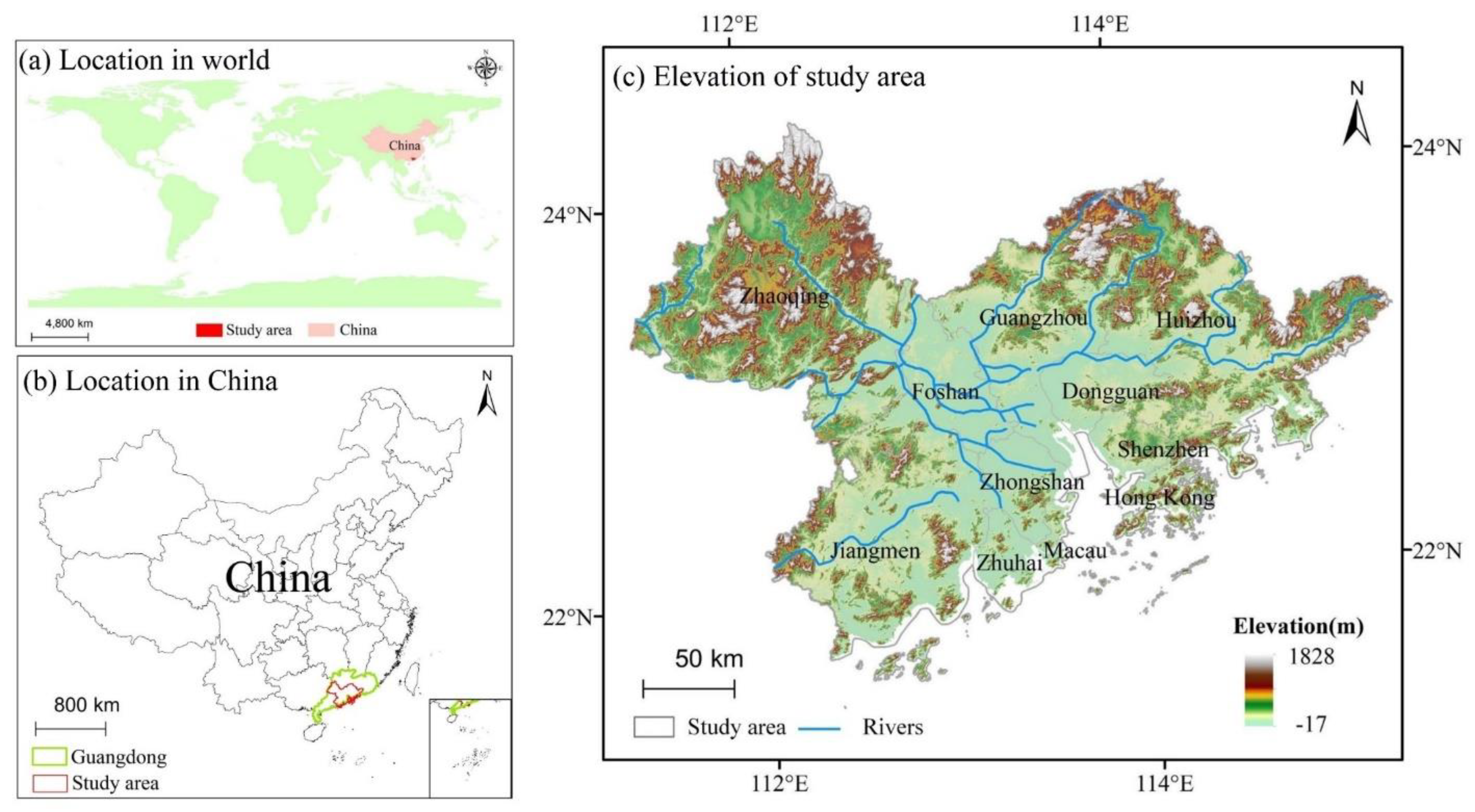
2.1. Study Area
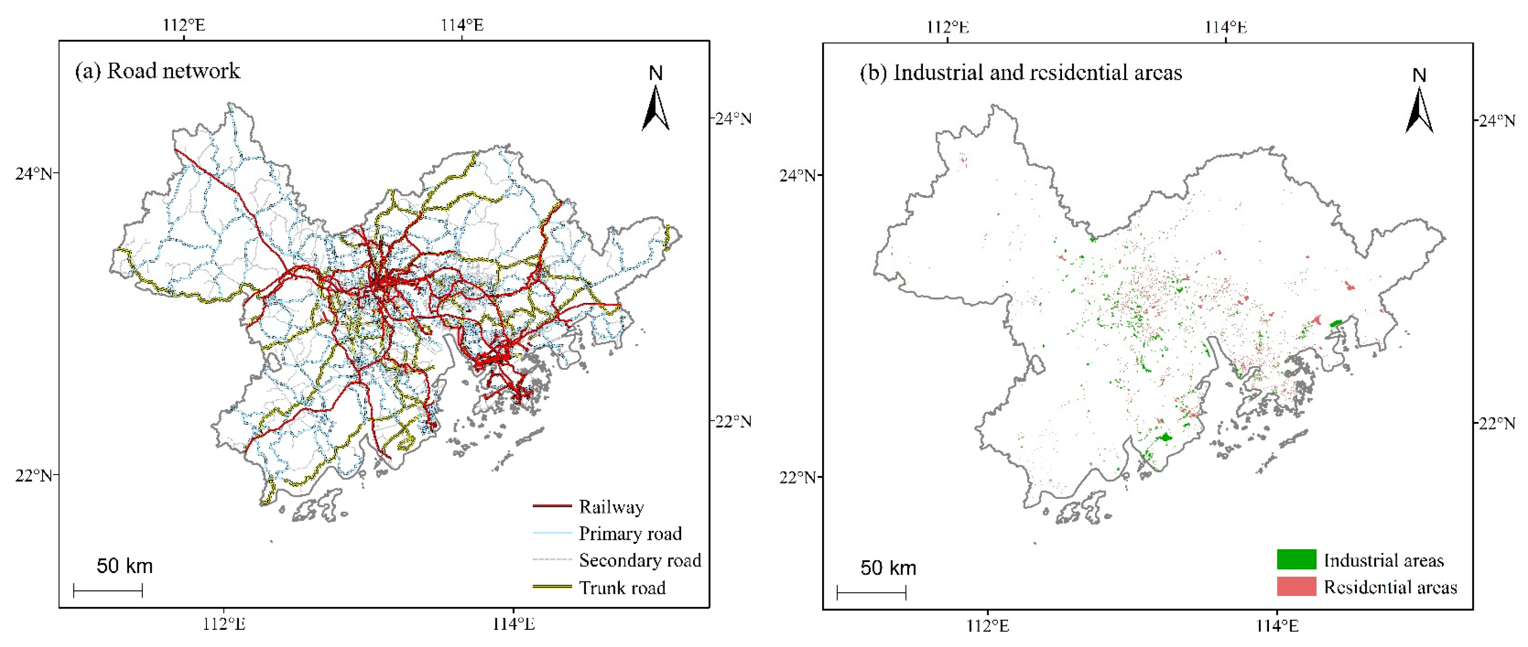
2.2. Data Resources and Preparation
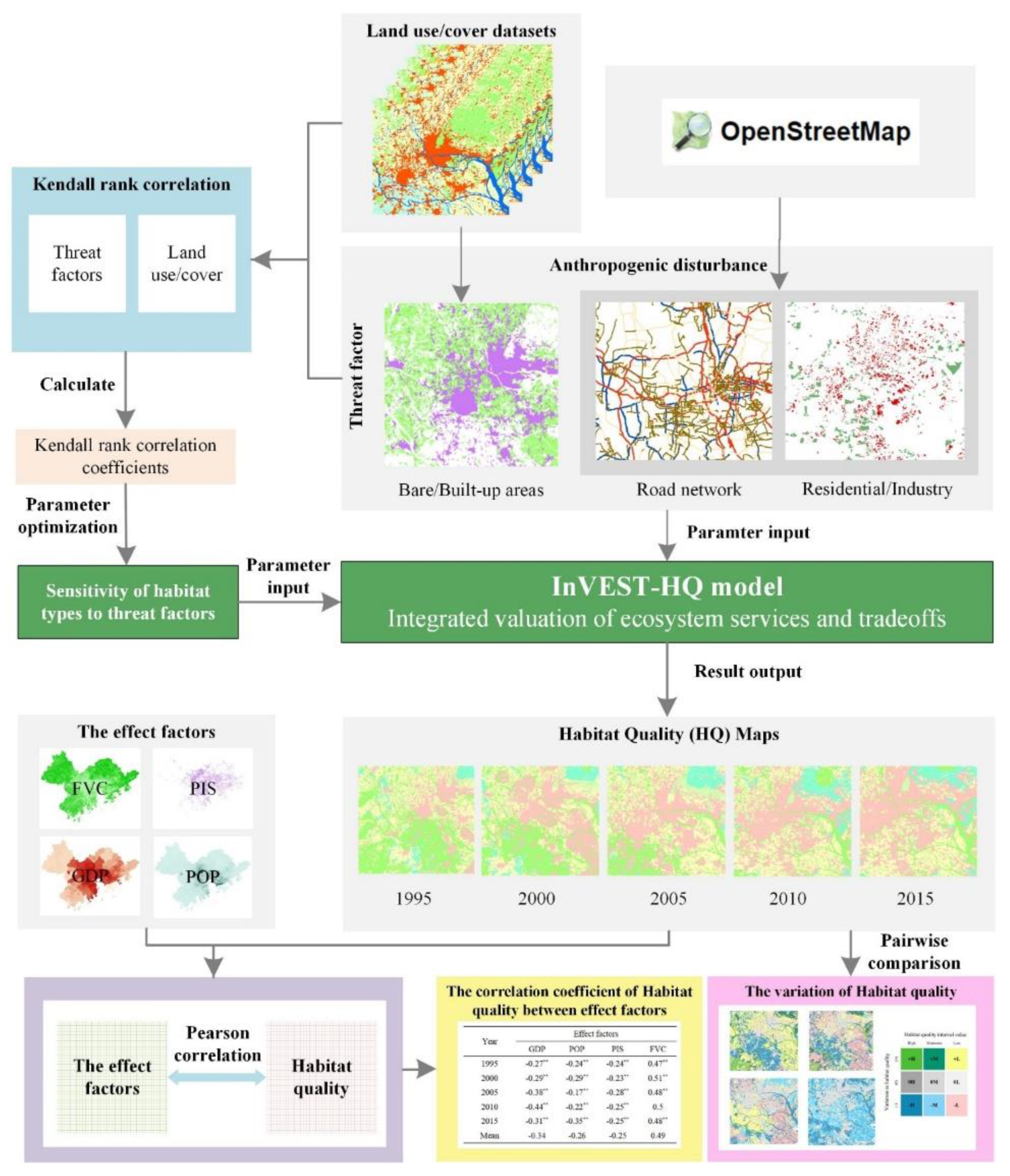
2.3. Methods
2.3.1. The InVEST Model
2.3.2. Kendall’s Rank Correlation Analysis Methods
2.3.3. Pearson’s Correlation Analysis Methods
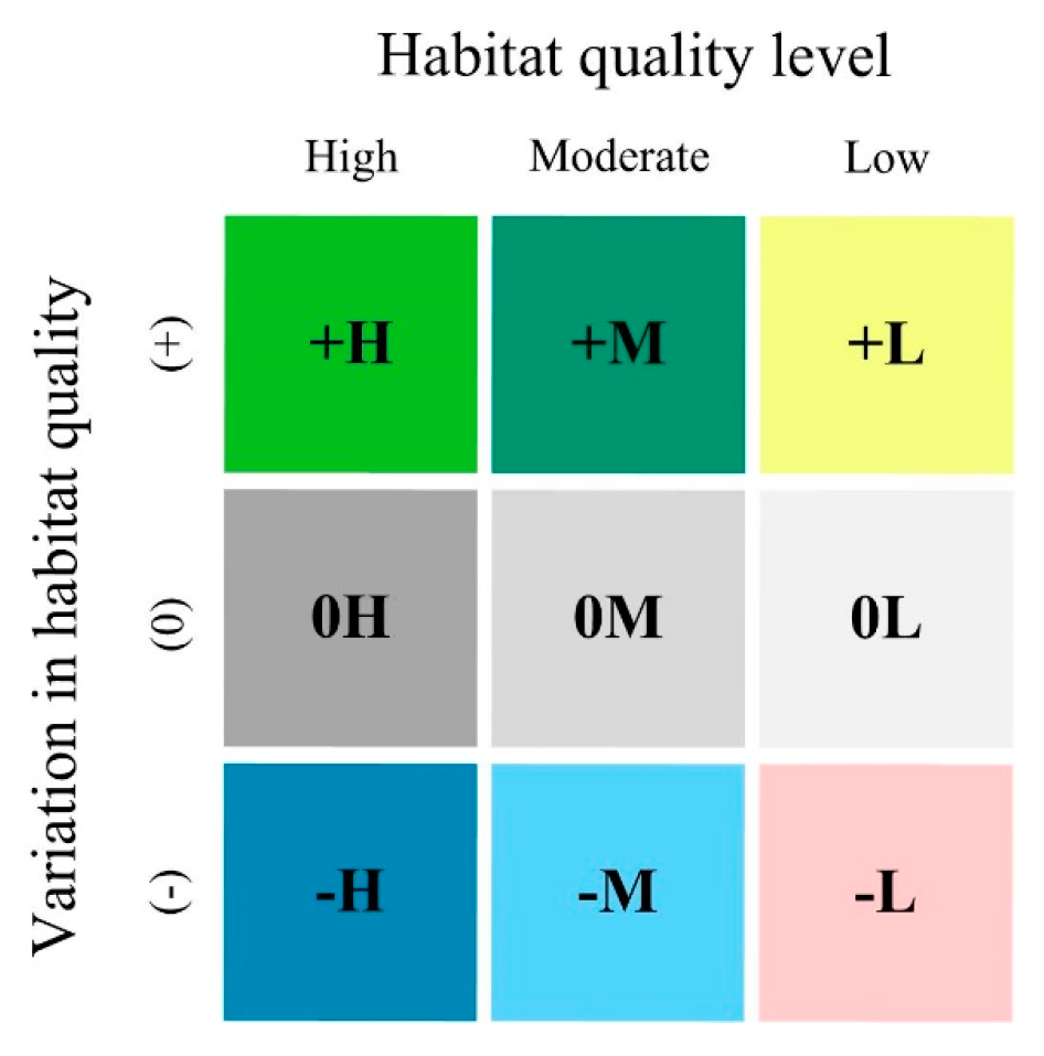
2.3.4. Variation in Habitat Quality Analysis
3. Model Parameter Settings
3.1. Threat Factor Parameters
3.2. Habitat Suitability Score
3.3. Sensitivity of Habitat Types to Threat Factors
4. Results and Analyses
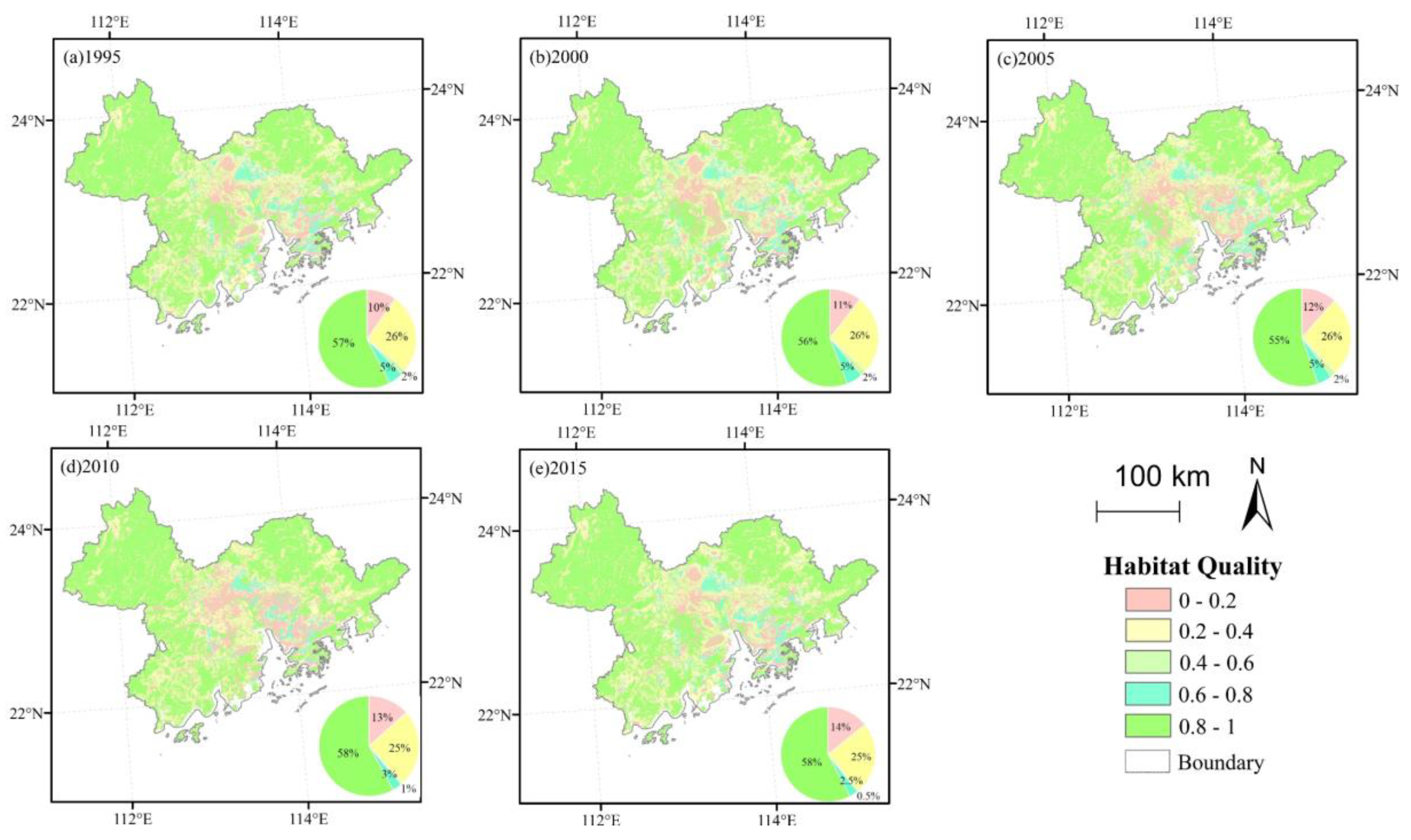
4.1. Characteristic of Spatiotemporal Pattern in Habitat Quality
4.1.1. Spatial Pattern of Habitat Quality
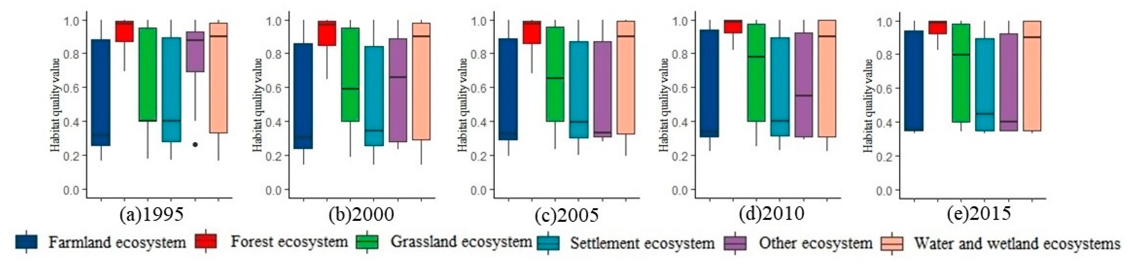
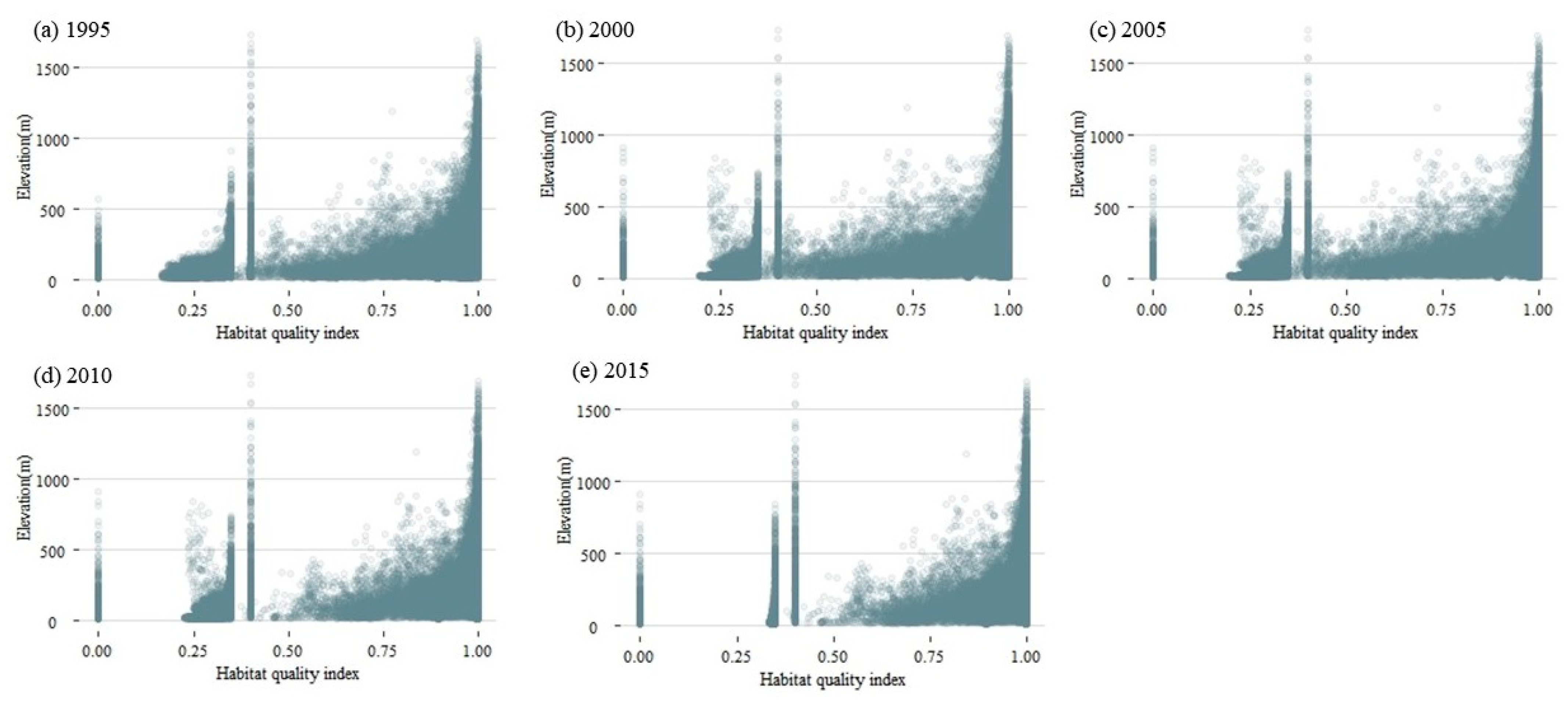
4.1.2. Spatial Pattern of Habitat Quality from Different Perspectives
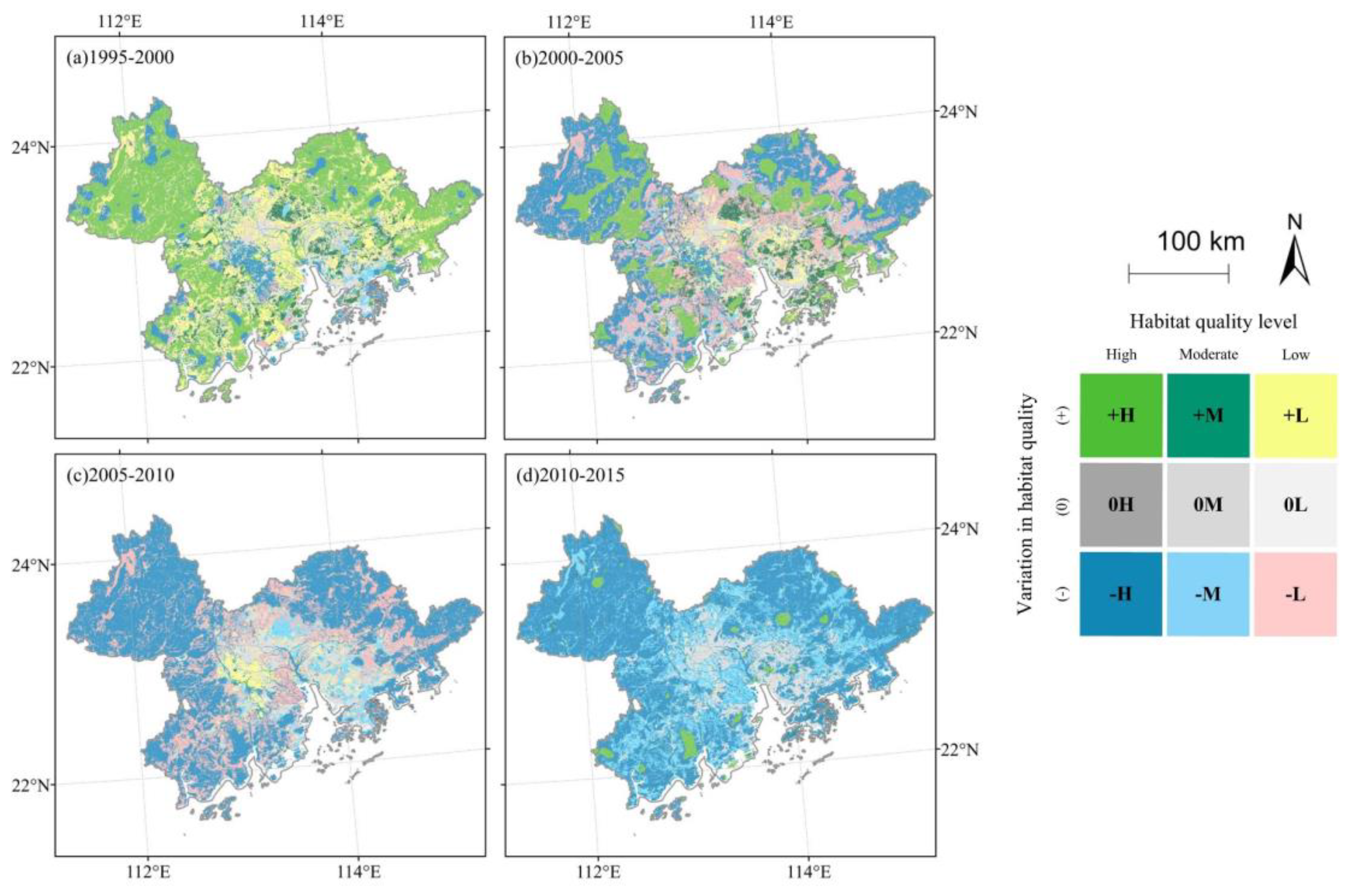
4.2. Characteristics of Spatiotemporal Variation in Habitat Quality
Spatiotemporal Variation of Habitat Quality
4.3. Analysis of the Variation of Habitat Quality and Effect Factor
5. Discussion
5.1. The Role of Sensitivity of Habitat Type to Threat Factors in the InVEST Habitat Quality Model
5.2. Exploring the Use of Assessment of Habitat Quality for Biodiversity Conservation
5.3. Limitations and Future Outlook
6. Conclusions
Author Contributions
Funding
Acknowledgments
Conflicts of Interest
Appendix A


| Year | LULC Types | Threat Factors | ||||||||
|---|---|---|---|---|---|---|---|---|---|---|
| Cropland | Built-Up Areas | Bare Land | Rail-Way | Trunk Road | Primary Road | Secondary Road | Industry Activity | Residential | ||
| 1995 | Cropland | 1 | 0.17 | 0.01 | 0.04 | 0.08 | 0.1 | 0.08 | 0.04 | 0.04 |
| Forest | 0.6 | 0.33 | 0.01 | 0.2 | 0.22 | 0.24 | 0.24 | 0.22 | 0.19 | |
| Grass land | 0.09 | 0.05 | 0 | 0.01 | 0.02 | 0.01 | 0.03 | 0.01 | 0.01 | |
| Wetland | 0.13 | 0.07 | 0 | 0.05 | 0.08 | 0.06 | 0.06 | 0.12 | 0.03 | |
| Water bodies | 0.08 | 0.05 | 0 | 0.02 | 0.04 | 0.03 | 0.02 | 0.07 | 0.01 | |
| Built-up areas | 0.17 | 1 | 0 | 0.25 | 0.24 | 0.26 | 0.29 | 0.19 | 0.27 | |
| Unused land | 0.01 | 0.01 | 0.35 | 0.01 | 0 | 0.01 | 0 | 0.02 | 0 | |
| 2000 | Cropland | 1 | 0.17 | 0.03 | 0.05 | 0.08 | 0.11 | 0.09 | 0.04 | 0.05 |
| Forest | 0.62 | 0.31 | 0.05 | 0.19 | 0.22 | 0.24 | 0.24 | 0.22 | 0.19 | |
| Grass land | 0.09 | 0.04 | 0.3 | 0.01 | 0.01 | 0.02 | 0.02 | 0.02 | 0.01 | |
| Wetland | 0.14 | 0.07 | 0.01 | 0.04 | 0.07 | 0.05 | 0.06 | 0.11 | 0.02 | |
| Water bodies | 0.09 | 0.04 | 0.01 | 0.02 | 0.04 | 0.02 | 0.01 | 0.06 | 0 | |
| Built-up areas | 0.17 | 1 | 0.01 | 0.24 | 0.24 | 0.25 | 0.28 | 0.19 | 0.27 | |
| Unused land | 0.01 | 0.01 | 0.21 | 0.01 | 0.01 | 0 | 0 | 0.01 | 0.01 | |
| 2005 | Cropland | 1 | 0.14 | 0 | 0 | 0.05 | 0.08 | 0.04 | 0.02 | 0.02 |
| Forest | 0.58 | 0.37 | 0.01 | 0.2 | 0.23 | 0.25 | 0.25 | 0.23 | 0.19 | |
| Grass land | 0.08 | 0.05 | 0 | 0.01 | 0.01 | 0.02 | 0.03 | 0.02 | 0.01 | |
| Wetland | 0.13 | 0.08 | 0 | 0.03 | 0.05 | 0.03 | 0.04 | 0.09 | 0.01 | |
| Water bodies | 0.08 | 0.05 | 0 | 0.02 | 0.04 | 0.02 | 0.01 | 0.06 | 0 | |
| Built-up areas | 0.15 | 1 | 0 | 0.24 | 0.24 | 0.25 | 0.28 | 0.19 | 0.24 | |
| Unused land | 0.01 | 0.01 | 0.77 | 0.01 | 0 | 0 | 0 | 0.01 | 0.01 | |
| 2010 | Cropland | 1 | 0.2 | 0 | 0 | 0.05 | 0.08 | 0.04 | 0.02 | 0.02 |
| Forest | 0.56 | 0.4 | 0.01 | 0.21 | 0.23 | 0.25 | 0.25 | 0.23 | 0.2 | |
| Grass land | 0.07 | 0.05 | 0 | 0.01 | 0.02 | 0.02 | 0.03 | 0.02 | 0.01 | |
| Wetland | 0.12 | 0.09 | 0 | 0.01 | 0.01 | 0 | 0 | 0.02 | 0.02 | |
| Water bodies | 0.08 | 0.06 | 0 | 0.02 | 0.04 | 0.03 | 0.01 | 0.06 | 0.01 | |
| Built-up areas | 0.2 | 1 | 0 | 0.3 | 0.28 | 0.3 | 0.35 | 0.28 | 0.29 | |
| Unused land | 0.01 | 0.01 | 0.69 | 0.01 | 0 | 0 | 0 | 0.01 | 0 | |
| 2015 | Cropland | 1 | 0.21 | 0 | 0.01 | 0.05 | 0.07 | 0.03 | 0.07 | 0.02 |
| Forest | 0.55 | 0.41 | 0.01 | 0.21 | 0.23 | 0.25 | 0.25 | 0.23 | 0.2 | |
| Grass land | 0.08 | 0.06 | 0 | 0.02 | 0.02 | 0.03 | 0.03 | 0.02 | 0.02 | |
| Wetland | 0.12 | 0.09 | 0 | 0.01 | 0.01 | 0 | 0 | 0.02 | 0.02 | |
| Water bodies | 0.08 | 0.06 | 0 | 0.02 | 0.04 | 0.03 | 0.01 | 0.06 | 0.01 | |
| Built-up areas | 0.21 | 1 | 0 | 0.31 | 0.29 | 0.3 | 0.36 | 0.29 | 0.29 | |
| Unused land | 0.01 | 0.01 | 0.72 | 0.01 | 0 | 0 | 0 | 0 | 0 | |
References
- Baeten, L.; Hermy, M.; Van Daele, S.; Verheyen, K. Unexpected understorey community development after 30 years in ancient and post-agricultural forests. J. Ecol. 2010, 98, 1447–1453. [Google Scholar] [CrossRef] [Green Version]
- Daskalova, G.N.; Myers-Smith, I.H.; Bjorkman, A.D.; Blowes, S.A.; Supp, S.R.; Magurran, A.E.; Dornelas, M. Landscape-scale forest loss as a catalyst of population and biodiversity change. Science 2020, 368, 1341–1347. [Google Scholar] [CrossRef]
- Newbold, T.; Hudson, L.N.; Hill, S.L.L.; Contu, S.; Lysenko, I.; Senior, R.A.; Börger, L.; Bennett, D.J.; Choimes, A.; Collen, B.; et al. Global effects of land use on local terrestrial biodiversity. Nat. Cell Biol. 2015, 520, 45–50. [Google Scholar] [CrossRef] [Green Version]
- Sallustio, L.; De Toni, A.; Strollo, A.; Di Febbraro, M.; Gissi, E.; Casella, L.; Geneletti, D.; Munafò, M.; Vizzarri, M.; Marchetti, M. Assessing habitat quality in relation to the spatial distribution of protected areas in Italy. J. Environ. Manag. 2017, 201, 129–137. [Google Scholar] [CrossRef]
- Ng, C.N.; Xie, Y.J.; Yu, X.J. Measuring the spatio-temporal variation of habitat isolation due to rapid urbanization: A case study of the Shenzhen River cross-boundary catchment, China. Landsc. Urban Plan. 2011, 103, 44–54. [Google Scholar] [CrossRef]
- Wilson, M.C.; Chen, X.-Y.; Corlett, R.T.; Didham, R.K.; Ding, P.; Holt, R.D.; Holyoak, M.; Hu, G.; Hughes, A.C.; Jiang, L.; et al. Erratum to: Habitat fragmentation and biodiversity conservation: Key findings and future challenges. Landsc. Ecol. 2015, 31, 229–230. [Google Scholar] [CrossRef] [Green Version]
- Bongaarts, J. IPBES, Summary for policymakers of the global assessment report on biodiversity and ecosystem services of the Intergov-ernmental Science-Policy Platform on Biodiversity and Ecosystem Services. Popul. Dev. Rev. 2019, 45, 680–681. [Google Scholar] [CrossRef] [Green Version]
- Oliver, T.H.; Heard, M.S.; Isaac, N.J.; Roy, D.B.; Procter, D.; Eigenbrod, F.; Freckleton, R.; Hector, A.; Orme, C.D.L.; Petchey, O.L.; et al. Biodiversity and Resilience of Ecosystem Functions. Trends Ecol. Evol. 2015, 30, 673–684. [Google Scholar] [CrossRef] [Green Version]
- Vellend, M.; Baeten, L.; Myers-Smith, I.H.; Elmendorf, S.C.; Beauséjour, R.; Brown, C.D.; De Frenne, P.; Verheyen, K.; Wipf, S. Global meta-analysis reveals no net change in local-scale plant biodiversity over time. Proc. Natl. Acad. Sci. USA 2013, 110, 19456–19459. [Google Scholar] [CrossRef] [PubMed] [Green Version]
- Dornelas, M.; Gotelli, N.J.; McGill, B.; Shimadzu, H.; Moyes, F.; Sievers, C.; Magurran, A.E. Assemblage Time Series Reveal Biodiversity Change but Not Systematic Loss. Science 2014, 344, 296–299. [Google Scholar] [CrossRef] [Green Version]
- Magurran, A.E.; Deacon, A.E.; Moyes, F.; Shimadzu, H.; Dornelas, M.; Phillip, D.A.T.; Ramnarine, I.W. Divergent biodiversity change within ecosystems. Proc. Natl. Acad. Sci. USA 2018, 115, 1843–1847. [Google Scholar] [CrossRef] [Green Version]
- Yoccoz, N.G.; Ellingsen, K.E.; Tveraa, T. Biodiversity may wax or wane depending on metrics or taxa. Proc. Natl. Acad. Sci. USA 2018, 115, 1681–1683. [Google Scholar] [CrossRef] [Green Version]
- Hall, L.S.; Krausman, P.R.; Morrison, M.L. The Habitat Concept and a Plea for Standard Terminology. Wildl. Soc. Bull. 1997, 25, 173–182. [Google Scholar]
- Terrado, M.; Sabater, S.; Chaplin-Kramer, B.; Mandle, L.; Ziv, G.; Acuña, V. Model development for the assessment of terrestrial and aquatic habitat quality in conservation planning. Sci. Total. Environ. 2016, 540, 63–70. [Google Scholar] [CrossRef] [Green Version]
- Thomas, J.A.; Bourn, N.A.D.; Clarke, R.T.; Stewart, K.E.; Simcox, D.J.; Pearman, G.S.; Curtis, R.; Goodger, B. The quality and isolation of habitat patches both determine where butterflies persist in fragmented landscapes. Proc. R. Soc. Lond. Ser. B Biol. Sci. 2001, 268, 1791–1796. [Google Scholar] [CrossRef]
- Fahrig, L. Effects of Habitat Fragmentation on Biodiversity. Annu. Rev. Ecol. Evol. Syst. 2003, 34, 487–515. [Google Scholar] [CrossRef] [Green Version]
- Howell, C.A.; Latta, S.C.; Donovan, T.M.; Porneluzi, P.A.; Parks, G.R.; Faaborg, J. Landscape effects mediate breeding bird abundance in midwestern forests. Landsc. Ecol. 2000, 15, 547–562. [Google Scholar] [CrossRef]
- Johnson, M.D. Measuring Habitat Quality: A Review. Condor 2007, 109, 489–504. [Google Scholar] [CrossRef]
- Sutherland, W.J. The effect of local change in habitat quality on populations of migratory species. J. Appl. Ecol. 1998, 35, 418–421. [Google Scholar] [CrossRef]
- Miller, J.R.; Groom, M.; Hess, G.R.; Steelman, T.; Stokes, D.L.; Thompson, J.; Bowman, T.; Fricke, L.; King, B.; Marquardt, R. Biodiversity Conservation in Local Planning. Conserv. Biol. 2009, 23, 53–63. [Google Scholar] [CrossRef] [PubMed]
- Beumer, L.T.; Van Beest, F.M.; Stelvig, M.; Schmidt, N.M. Spatiotemporal dynamics in habitat suitability of a large Arctic herbivore: Environmental heterogeneity is key to a sedentary lifestyle. Glob. Ecol. Conserv. 2019, 18, e00647. [Google Scholar] [CrossRef]
- Srivastava, V.; Griess, V.C.; Padalia, H. Mapping invasion potential using ensemble modelling. A case study on Yushania maling in the Darjeeling Himalayas. Ecol. Model. 2018, 385, 35–44. [Google Scholar] [CrossRef]
- Elith, J.; Leathwick, J.R. Species Distribution Models: Ecological Explanation and Prediction Across Space and Time. Annu. Rev. Ecol. Evol. Syst. 2009, 40, 677–697. [Google Scholar] [CrossRef]
- Mocq, J.; St-Hilaire, A.; Cunjak, R. Assessment of Atlantic salmon (Salmo salar) habitat quality and its uncertainty using a multiple-expert fuzzy model applied to the Romaine River (Canada). Ecol. Model. 2013, 265, 14–25. [Google Scholar] [CrossRef]
- Sharp, R.; Douglass, J.; Wolny, S.; Arkema, K.; Bernhardt, J.; Bierbower, W.; Chaumont, N.; Denu, D.; Fisher, D.; Glowinski, K.; et al. InVEST 3.8.7. User’s Guide; Collaborative publication by The Natural Capital Project, Stanford University, University of Minnesota, The Nature Conservancy, and World Wildlife Fund; Stanford University: Stanford, CA, USA, 2020. [Google Scholar]
- Alkemade, R.; Van Oorschot, M.; Miles, L.; Nellemann, C.; Bakkenes, M.; Brink, B.T. GLOBIO3: A Framework to Investigate Options for Reducing Global Terrestrial Biodiversity Loss. Ecosystems 2009, 12, 374–390. [Google Scholar] [CrossRef] [Green Version]
- Zhu, C.; Zhang, X.; Zhou, M.; He, S.; Gan, M.; Yang, L.; Wang, K. Impacts of urbanization and landscape pattern on habitat quality using OLS and GWR models in Hangzhou, China. Ecol. Indic. 2020, 117, 106654. [Google Scholar] [CrossRef]
- Chiang, L.-C.; Lin, Y.-P.; Huang, T.; Schmeller, D.S.; Verburg, P.H.; Liu, Y.-L.; Ding, T.-S. Simulation of ecosystem service responses to multiple disturbances from an earthquake and several typhoons. Landsc. Urban Plan. 2014, 122, 41–55. [Google Scholar] [CrossRef]
- Xu, L.; Chen, S.S.; Xu, Y.; Li, G.; Su, W. Impacts of Land-Use Change on Habitat Quality during 1985–2015 in the Taihu Lake Basin. Sustainability 2019, 11, 3513. [Google Scholar] [CrossRef] [Green Version]
- Sun, X.; Jiang, Z.; Liu, F.; Zhang, D. Monitoring spatio-temporal dynamics of habitat quality in Nansihu Lake basin, eastern China, from 1980 to 2015. Ecol. Indic. 2019, 102, 716–723. [Google Scholar] [CrossRef]
- Hack, J.; Molewijk, D.; Beißler, M.R. A Conceptual Approach to Modeling the Geospatial Impact of Typical Urban Threats on the Habitat Quality of River Corridors. Remote Sens. 2020, 12, 1345. [Google Scholar] [CrossRef] [Green Version]
- Song, S.; Liu, Z.; He, C.; Lu, W. Evaluating the effects of urban expansion on natural habitat quality by coupling localized shared socioeconomic pathways and the land use scenario dynamics-urban model. Ecol. Indic. 2020, 112, 106071. [Google Scholar] [CrossRef]
- Ma, Y.; Zhang, S.; Yang, K.; Li, M. Influence of spatiotemporal pattern changes of impervious surface of urban megaregion on thermal environment: A case study of the Guangdong—Hong Kong—Macao Greater Bay Area of China. Ecol. Indic. 2021, 121, 107106. [Google Scholar] [CrossRef]
- Bi, M.; Xie, G.; Yao, C. Ecological security assessment based on the renewable ecological footprint in the Guangdong-Hong Kong-Macao Greater Bay Area, China. Ecol. Indic. 2020, 116, 106432. [Google Scholar] [CrossRef]
- Ma, P.; Wang, W.; Zhang, B.; Wang, J.; Shi, G.; Huang, G.; Chen, F.; Jiang, L.; Lin, H. Remotely sensing large- and small-scale ground subsidence: A case study of the Guangdong–Hong Kong–Macao Greater Bay Area of China. Remote Sens. Environ. 2019, 232, 111282. [Google Scholar] [CrossRef]
- Wu, M.; Wu, J.; Zang, C. A comprehensive evaluation of the eco-carrying capacity and green economy in the Guangdong-Hong Kong-Macao Greater Bay Area, China. J. Clean. Prod. 2021, 281, 124945. [Google Scholar] [CrossRef]
- Liu, J.; Zhang, Z.; Xu, X.; Kuang, W.; Zhou, W.; Zhang, S.; Li, R.; Yan, C.; Yu, D.; Wu, S.; et al. Spatial patterns and driving forces of land use change in China during the early 21st century. J. Geogr. Sci. 2010, 20, 483–494. [Google Scholar] [CrossRef]
- Gong, P.; Li, X.; Wang, J.; Bai, Y.; Chen, B.; Hu, T.; Liu, X.; Xu, B.; Yang, J.; Zhang, W.; et al. Annual maps of global artificial impervious area (GAIA) between 1985 and 2018. Remote Sens. Environ. 2020, 236, 111510. [Google Scholar] [CrossRef]
- Bhagabati, N.K.; Ricketts, T.H.; Sulistyawan, T.B.S.; Conte, M.; Ennaanay, D.; Hadian, O.; McKenzie, E.; Olwero, N.; Rosenthal, A.; Tallis, H.; et al. Ecosystem services reinforce Sumatran tiger conservation in land use plans. Biol. Conserv. 2014, 169, 147–156. [Google Scholar] [CrossRef]
- Czekajlo, A.; Coops, N.C.; Wulder, M.A.; Hermosilla, T.; Lu, Y.; White, J.C.; Bosch, M.V.D. The urban greenness score: A satellite-based metric for multi-decadal characterization of urban land dynamics. Int. J. Appl. Earth Obs. Geoinform. 2020, 93, 102210. [Google Scholar] [CrossRef]
- Anchang, J.Y.; Ananga, E.O.; Pu, R. An efficient unsupervised index based approach for mapping urban vegetation from IKONOS imagery. Int. J. Appl. Earth Obs. Geoinform. 2016, 50, 211–220. [Google Scholar] [CrossRef]
- He, J.; Huang, J.; Li, C. The evaluation for the impact of land use change on habitat quality: A joint contribution of cellular automata scenario simulation and habitat quality assessment model. Ecol. Model. 2017, 366, 58–67. [Google Scholar] [CrossRef]
- Huang, J.; Tang, Z.; Liu, D.; He, J. Ecological response to urban development in a changing socio-economic and climate context: Policy implications for balancing regional development and habitat conservation. Land Use Policy 2020, 97, 104772. [Google Scholar] [CrossRef]
- Weng, Q. Land use change analysis in the Zhujiang Delta of China using satellite remote sensing, GIS and stochastic modelling. J. Environ. Manag. 2002, 64, 273–284. [Google Scholar] [CrossRef] [Green Version]
- Foley, J.A.; DeFries, R.; Asner, G.P.; Barford, C.; Bonan, G.; Carpenter, S.R.; Chapin, F.S.; Coe, M.T.; Daily, G.C.; Gibbs, H.K.; et al. Global Consequences of Land Use. Science 2005, 309, 570–574. [Google Scholar] [CrossRef] [PubMed] [Green Version]
- Benítez-López, A.; Alkemade, R.; Verweij, P.A. The impacts of roads and other infrastructure on mammal and bird populations: A meta-analysis. Biol. Conserv. 2010, 143, 1307–1316. [Google Scholar] [CrossRef] [Green Version]
- Nematollahi, S.; Fakheran, S.; Kienast, F.; Jafari, A. Application of InVEST habitat quality module in spatially vulnerability assessment of natural habitats (case study: Chaharmahal and Bakhtiari province, Iran). Environ. Monit. Assess. 2020, 192, 1–17. [Google Scholar] [CrossRef]
- Selva, N.; Kreft, S.; Kati, V.; Schluck, M.; Jonsson, B.-G.; Mihok, B.; Okarma, H.; Ibisch, P.L. Roadless and Low-Traffic Areas as Conservation Targets in Europe. Environ. Manag. 2011, 48, 865–877. [Google Scholar] [CrossRef] [Green Version]
- Aneseyee, A.B.; Noszczyk, T.; Soromessa, T.; Elias, E. The InVEST Habitat Quality Model Associated with Land Use/Cover Changes: A Qualitative Case Study of the Winike Watershed in the Omo-Gibe Basin, Southwest Ethiopia. Remote Sens. 2020, 12, 1103. [Google Scholar] [CrossRef] [Green Version]
- Li, F.; Wang, L.; Chen, Z.; Clarke, K.C.; Li, M.; Jiang, P. Extending the SLEUTH model to integrate habitat quality into urban growth simulation. J. Environ. Manag. 2018, 217, 486–498. [Google Scholar] [CrossRef] [PubMed] [Green Version]
- Zhai, T.; Wang, J.; Fang, Y.; Qin, Y.; Huang, L.; Chen, Y. Assessing ecological risks caused by human activities in rapid urbanization coastal areas: Towards an integrated approach to determining key areas of terrestrial-oceanic ecosystems preservation and restoration. Sci. Total Environ. 2020, 708, 135153. [Google Scholar] [CrossRef] [PubMed]
- Yang, C.; Li, Q.; Hu, Z.; Chen, J.; Shi, T.; Ding, K.; Wu, G. Spatiotemporal evolution of urban agglomerations in four major bay areas of US, China and Japan from 1987 to 2017: Evidence from remote sensing images. Sci. Total Environ. 2019, 671, 232–247. [Google Scholar] [CrossRef] [PubMed]
- Derumigny, A.; Fermanian, J.-D. A classification point-of-view about conditional Kendall’s tau. Comput. Stat. Data Anal. 2019, 135, 70–94. [Google Scholar] [CrossRef] [Green Version]
- Mendes, R.S.; Lush, V.; Wanner, E.F.; Martins, F.V.; Sarubbi, J.F.; Deb, K. Online clustering reduction based on parametric and non-parametric correlation for a many-objective vehicle routing problem with demand responsive transport. Expert Syst. Appl. 2021, 170, 114467. [Google Scholar] [CrossRef]
- Sepúlveda, A.; Guido, R.C.; Castellanos-Dominguez, G. Estimation of relevant time–frequency features using Kendall coefficient for articulator position inference. Speech Commun. 2013, 55, 99–110. [Google Scholar] [CrossRef]
- McKinney, M.L. Urbanization, Biodiversity, and Conservation: The impacts of urbanization on native species are poorly studied, but educating a highly urbanized human population about these impacts can greatly improve species conserva-tion in all ecosystems. BioScience 2002, 52, 883–890. [Google Scholar] [CrossRef]
- Coffin, A.W. From roadkill to road ecology: A review of the ecological effects of roads. J. Transp. Geogr. 2007, 15, 396–406. [Google Scholar] [CrossRef]
- Gong, J.; Xie, Y.; Cao, E.; Huang, Q.; Li, H. Integration of InVEST-habitat quality model with landscape pattern indexes to assess mountain plant biodiversity change: A case study of Bailongjiang watershed in Gansu Province. J. Geogr. Sci. 2019, 29, 1193–1210. [Google Scholar] [CrossRef] [Green Version]
- Tang, Z.; Ma, J.; Peng, H.; Wang, S.; Wei, J. Spatiotemporal changes of vegetation and their responses to temperature and precipitation in upper Shiyang river basin. Adv. Space Res. 2017, 60, 969–979. [Google Scholar] [CrossRef]
- Zhu, J.; Ding, N.; Li, D.; Sun, W.; Xie, Y.; Wang, X. Spatiotemporal Analysis of the Nonlinear Negative Relationship between Urbanization and Habitat Quality in Metropolitan Areas. Sustainability 2020, 12, 669. [Google Scholar] [CrossRef] [Green Version]
- Polasky, S.; Nelson, E.; Pennington, D.; Johnson, K.A. The Impact of Land-Use Change on Ecosystem Services, Biodiversity and Returns to Landowners: A Case Study in the State of Minnesota. Environ. Resour. Econ. 2010, 48, 219–242. [Google Scholar] [CrossRef]
- Yohannes, H.; Soromessa, T.; Argaw, M.; Dewan, A. Spatio-temporal changes in habitat quality and linkage with landscape characteristics in the Beressa watershed, Blue Nile basin of Ethiopian highlands. J. Environ. Manag. 2021, 281, 111885. [Google Scholar] [CrossRef] [PubMed]
- Di Febbraro, M.; Sallustio, L.; Vizzarri, M.; De Rosa, D.; De Lisio, L.; Loy, A.; Eichelberger, B.; Marchetti, M. Expert-based and correlative models to map habitat quality: Which gives better support to conservation planning? Glob. Ecol. Conserv. 2018, 16, e00513. [Google Scholar] [CrossRef]


| No. | Datasets | Data Description | Data Resources | Data Format |
|---|---|---|---|---|
| 1 | Land use/cover datasets | China land use/cover change data | Obtained from Resources and Environmental Sciences, Chinese Academy of Sciences (RESDC), http://www.resdc.cn, DataID = 184 (accessed on 20 January 2021) | TIFF |
| 2 | Vector datasets | Road network datasets, residential datasets and industry datasets obtained | Obtained from OpenStreetMap (OSM), https://download.geofabrik.de/ (accessed on 20 January 2021) | Shapefile |
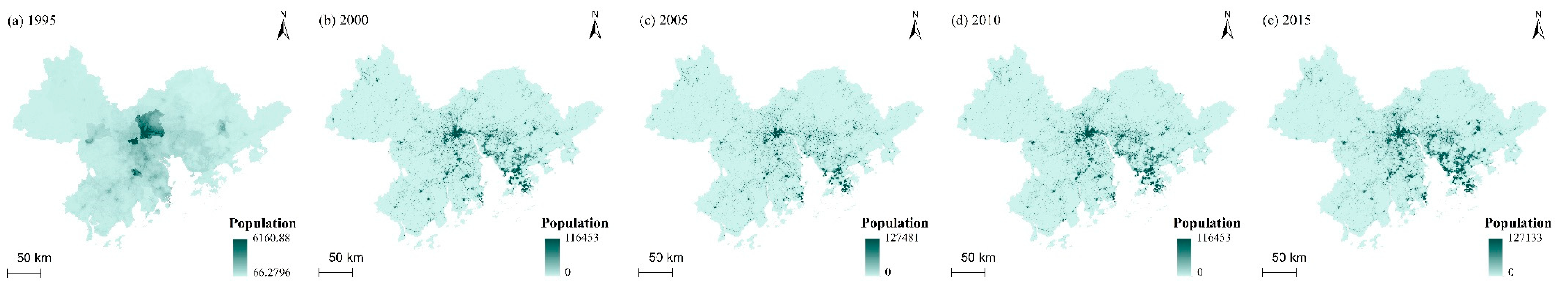
| 3 | Socioeconomic datasets | Population distribution (POP) data | Obtained from Oak Ridge National Laborator LandScan global population distribution data, https://landscan.ornl.gov/landscan-datasets (accessed on 20 January 2021) | TIFF |
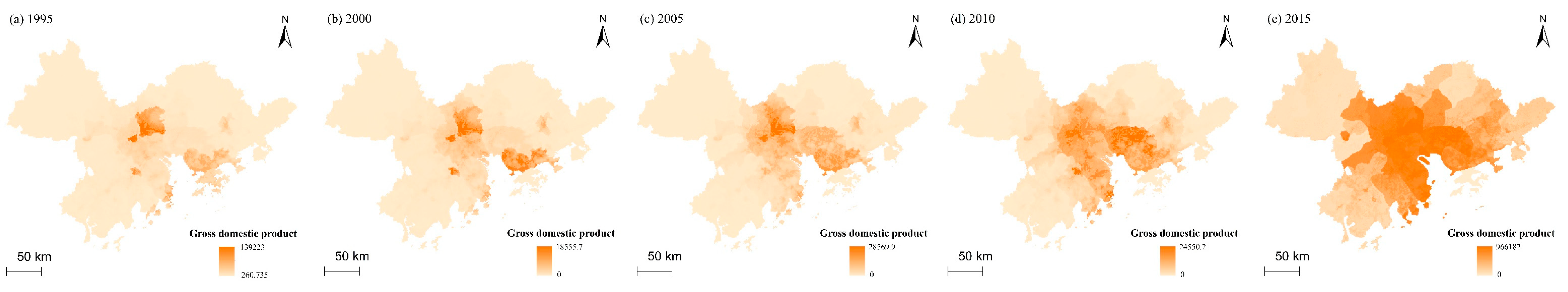
| Gross domestic product (GDP) data | Obtained from RESDC 1 km grid GDP data, http://www.resdc.cn/data.aspx?DATAID=252 (accessed on 20 January 2021) | TIFF | ||
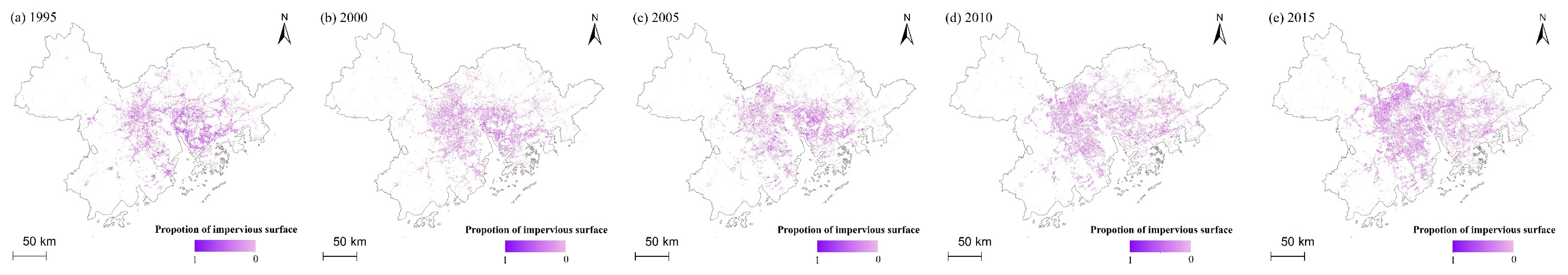
| 4 | Impervious surface data | Global artificial impervious data | Obtained from global artificial impervious area (GAIA) maps, http://data.ess.tsinghua.edu.cn/gaia.html (accessed on 20 January 2021) | TIFF |
| 5 | Normalized difference vegetation index data | MOD13Q1 16-day products and RESDC NDVI dataset | Obtained from Level-1 and Atmosphere Archive & Distribution System Distributed Active Archive Center (LAADS DAAC) (https://ladsweb.modaps.eosdis.nasa.gov/ (accessed on 20 January 2021)) and RESDC (http://www.resdc.cn/DOI/doi.aspx?DOIid=49 (accessed on 20 January 2021)) | TIFF |
| 6 | Supplementary analysis datasets | DEM data | the Shuttle Radar Topography Mission (SRTM), http://srtm.csi.cgiar.org/srtmdata/ (accessed on 20 January 2021) | TIFF |
| Terrestrial ecosystem classification data | Obtained from RESDC, http://www.resdc.cn/DOI/doi.aspx?DOIid=103 (accessed on 20 January 2021) | TIFF |
| Parameter | Parameter Description | Data Resources | Data Format |
|---|---|---|---|
| LULC | Land use/cover map | CNLUCC | TIFF |
| Threat factor | The layer of threat factor | OSM and CNLUCC | Transferred to TIFF |
| Threat factor parameters | The weight of threat factor | Based on relevant literature [4,27,30,31] and InVEST user’s guide [25] | CSV |
| The maximum distance of each threat factor | |||
| The types of decay over space for the threat | |||
| Habitat suitability score | Each LULC type needs to give a habitat suitability score with a value ranging from 0 to 1 | Based on relevant literature [4,27] and InVEST user’s guide [25] | CSV |
| Sensitivity of habitat types to threat factors | The parameter of the sensitivity score for LULC to the threat factor | The absolute value of Kendall’s correlation coefficients | CSV |
| Threat | Weight | Maximum Distance | Decay Type |
|---|---|---|---|
| Bare land | 0.2 | 3 | linear |
| Built-up areas | 1 | 10 | exponential |
| Cropland | 0.68 | 8 | linear |
| Railway | 0.9 | 9 | exponential |
| Trunk road | 1 | 10 | exponential |
| Primary road | 1 | 8 | linear |
| Secondary road | 0.75 | 5 | linear |
| Industry activity | 1 | 12 | exponential |
| Residential | 0.5 | 5 | exponential |
| LULC Types | Cropland | Forest | Grassland | Water Bodies | Wetland | Built-Up Areas | Unused Land |
|---|---|---|---|---|---|---|---|
| Habitat score | 0.35 | 1 | 0.4 | 0.9 | 1 | 0 | 0 |
| Year | Effect Factors | |||
|---|---|---|---|---|
| GDP | POP | PIS | FVC | |
| 1995 | −0.27 ** | −0.24 ** | −0.24 ** | 0.47 ** |
| 2000 | −0.29 ** | −0.29 ** | −0.23 ** | 0.51 ** |
| 2005 | −0.38 ** | −0.17 ** | −0.28 ** | 0.48 ** |
| 2010 | −0.44 ** | −0.22 ** | −0.25 ** | 0.5 |
| 2015 | −0.31 ** | −0.35 ** | −0.25 ** | 0.48 ** |
| Mean | −0.34 | −0.26 | −0.25 | 0.49 |
Publisher’s Note: MDPI stays neutral with regard to jurisdictional claims in published maps and institutional affiliations. |
© 2021 by the authors. Licensee MDPI, Basel, Switzerland. This article is an open access article distributed under the terms and conditions of the Creative Commons Attribution (CC BY) license (http://creativecommons.org/licenses/by/4.0/).
Share and Cite
Wu, L.; Sun, C.; Fan, F. Estimating the Characteristic Spatiotemporal Variation in Habitat Quality Using the InVEST Model—A Case Study from Guangdong–Hong Kong–Macao Greater Bay Area. Remote Sens. 2021, 13, 1008. https://doi.org/10.3390/rs13051008
Wu L, Sun C, Fan F. Estimating the Characteristic Spatiotemporal Variation in Habitat Quality Using the InVEST Model—A Case Study from Guangdong–Hong Kong–Macao Greater Bay Area. Remote Sensing. 2021; 13(5):1008. https://doi.org/10.3390/rs13051008
Chicago/Turabian StyleWu, Linlin, Caige Sun, and Fenglei Fan. 2021. "Estimating the Characteristic Spatiotemporal Variation in Habitat Quality Using the InVEST Model—A Case Study from Guangdong–Hong Kong–Macao Greater Bay Area" Remote Sensing 13, no. 5: 1008. https://doi.org/10.3390/rs13051008