
Soil Moisture Estimation Synergy Using GNSS-R and L-Band Microwave Radiometry Data from FSSCat/FMPL-2

 ,
,  , , , and
Abstract
:
1. Introduction
2. Data Description
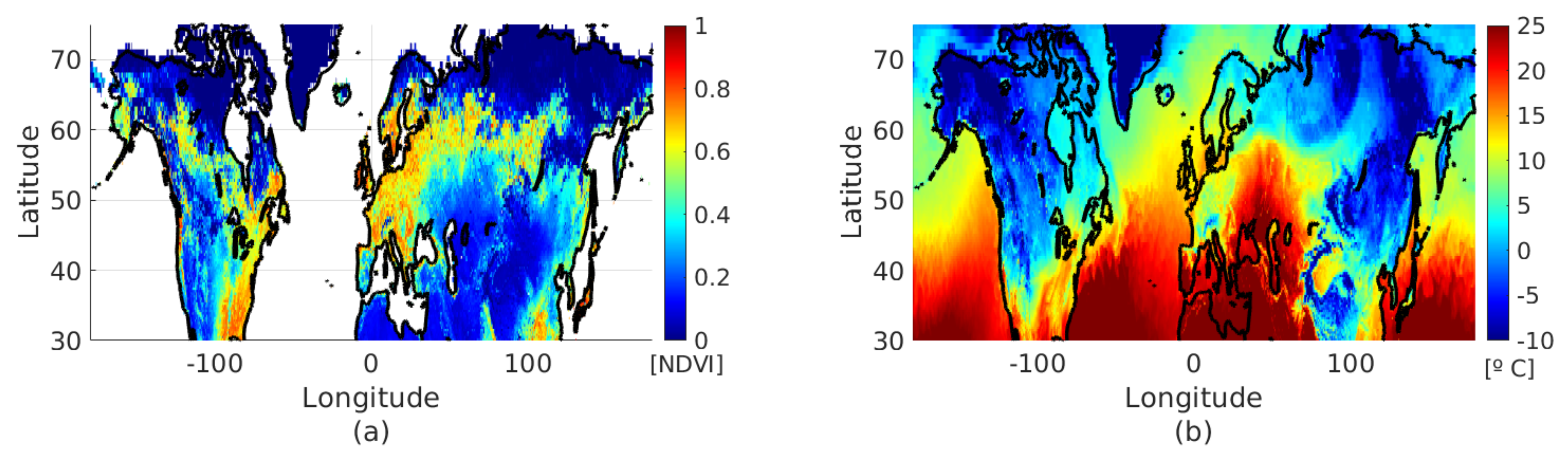
2.1. Ancillary Data
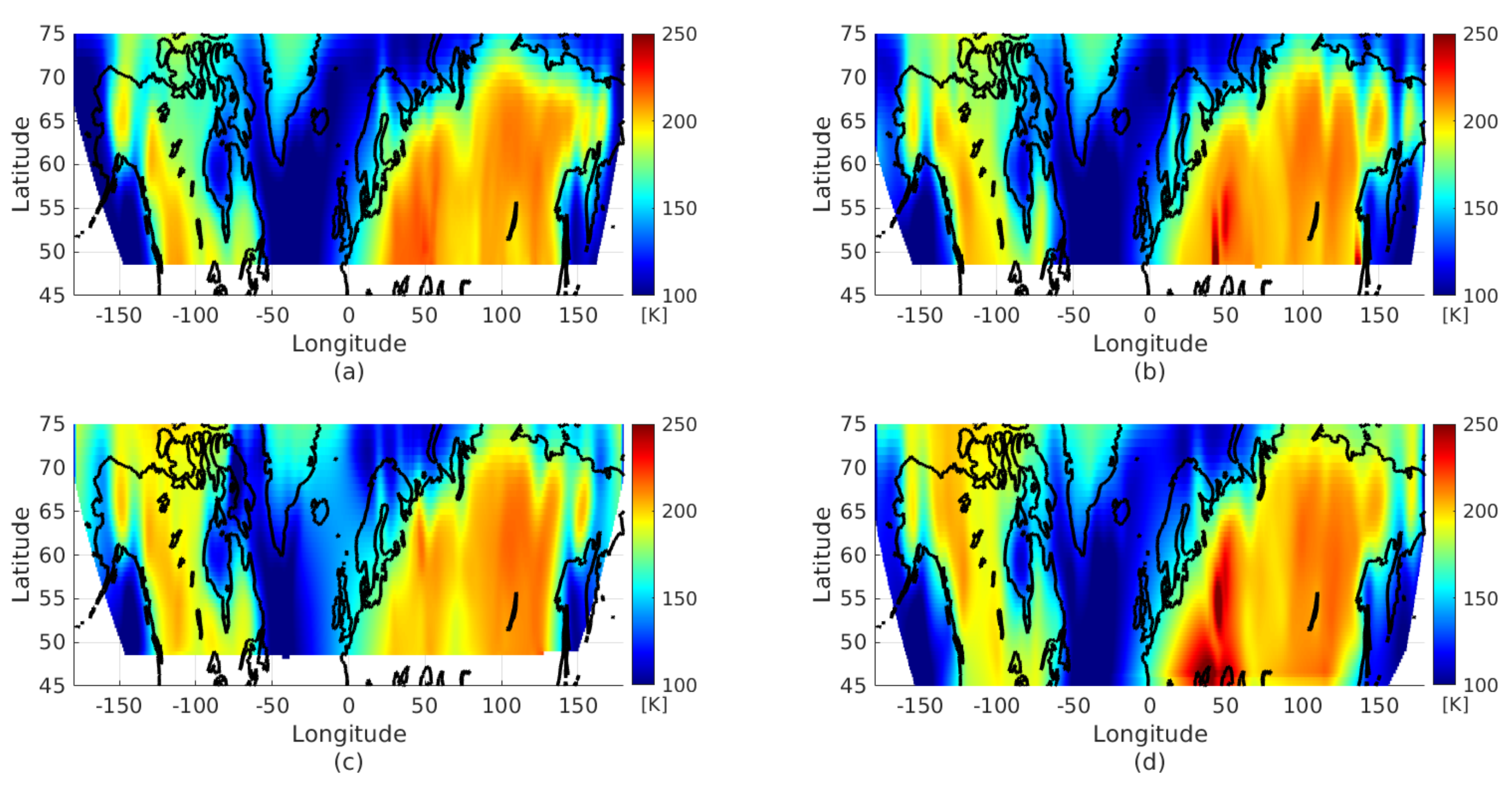
2.2. FMPL-2 Data
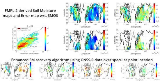
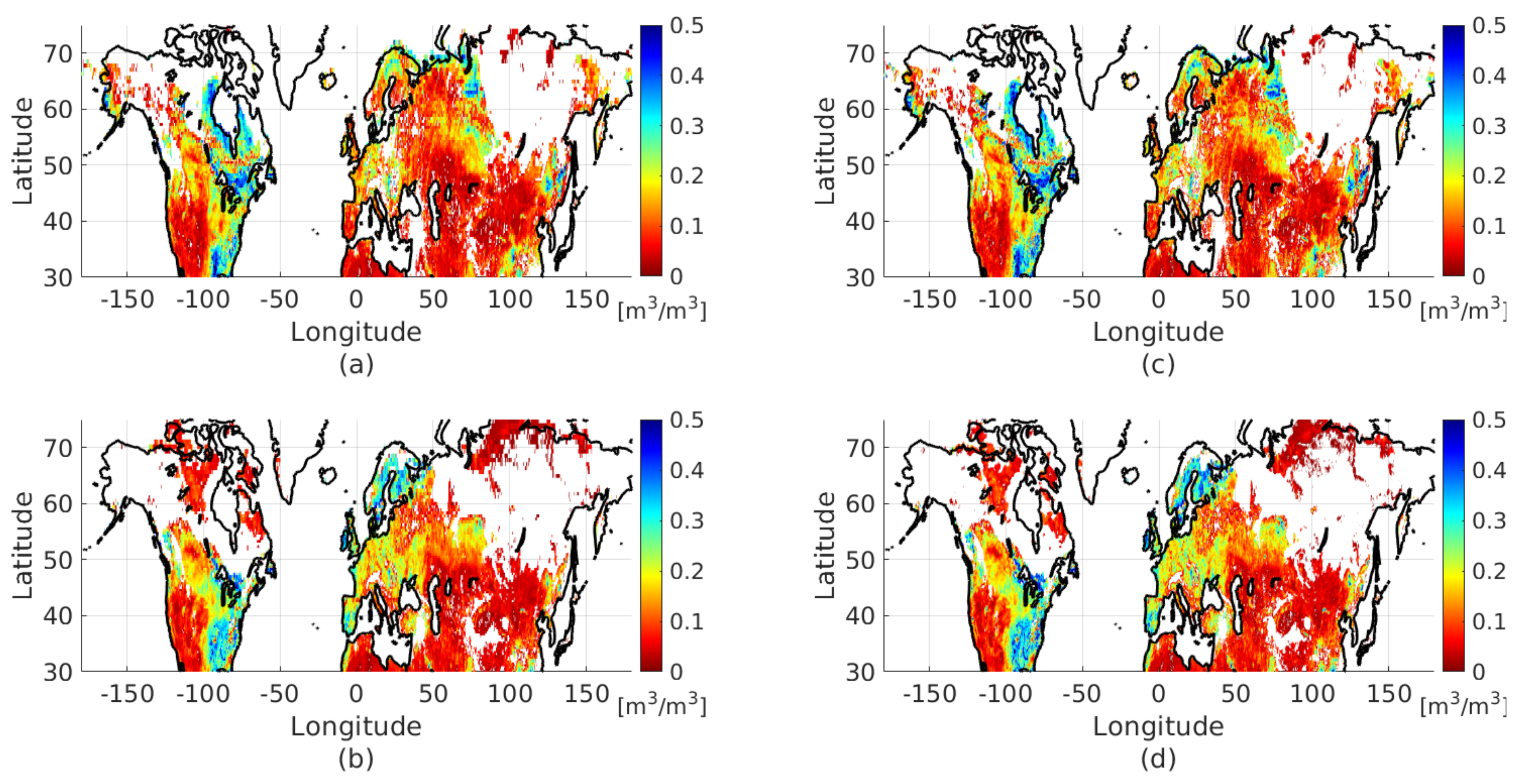
3. Soil Moisture Retrieval Using ANN
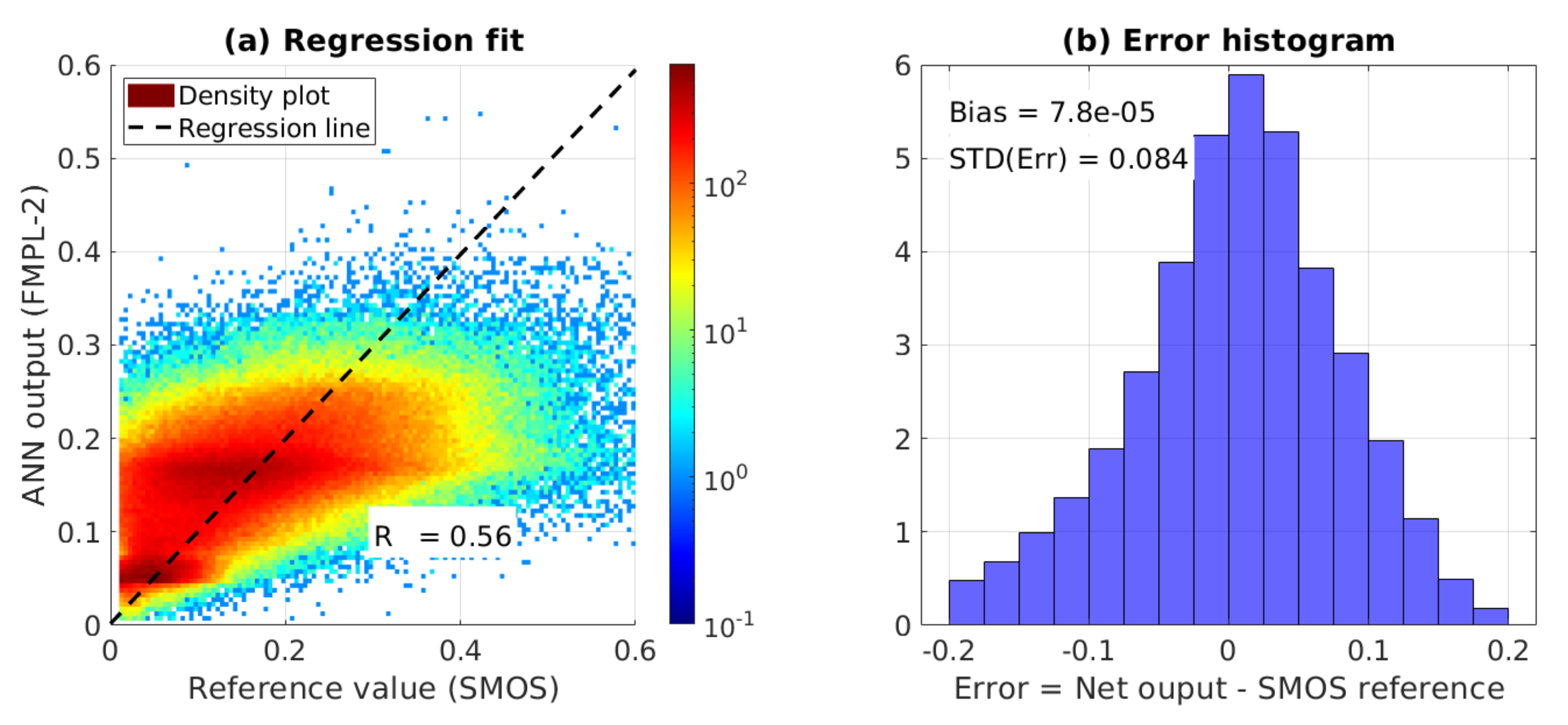
3.1. Using Optical Data
3.2. Using L-Band Microwave Radiometry Data
- FMPL-2 antenna temperature,
- FMPL-2 standard deviation of the antenna temperature in the along-track measurement,
- NDVI from MODIS [49],
- Low resolution NDVI from MODIS [49],
- Skin temperature from ECMWF [50],
- Low resolution skin temperature from ECMWF [50],
- Land cover mask from MODIS [49], and
- Low resolution land cover mask from MODIS [49].
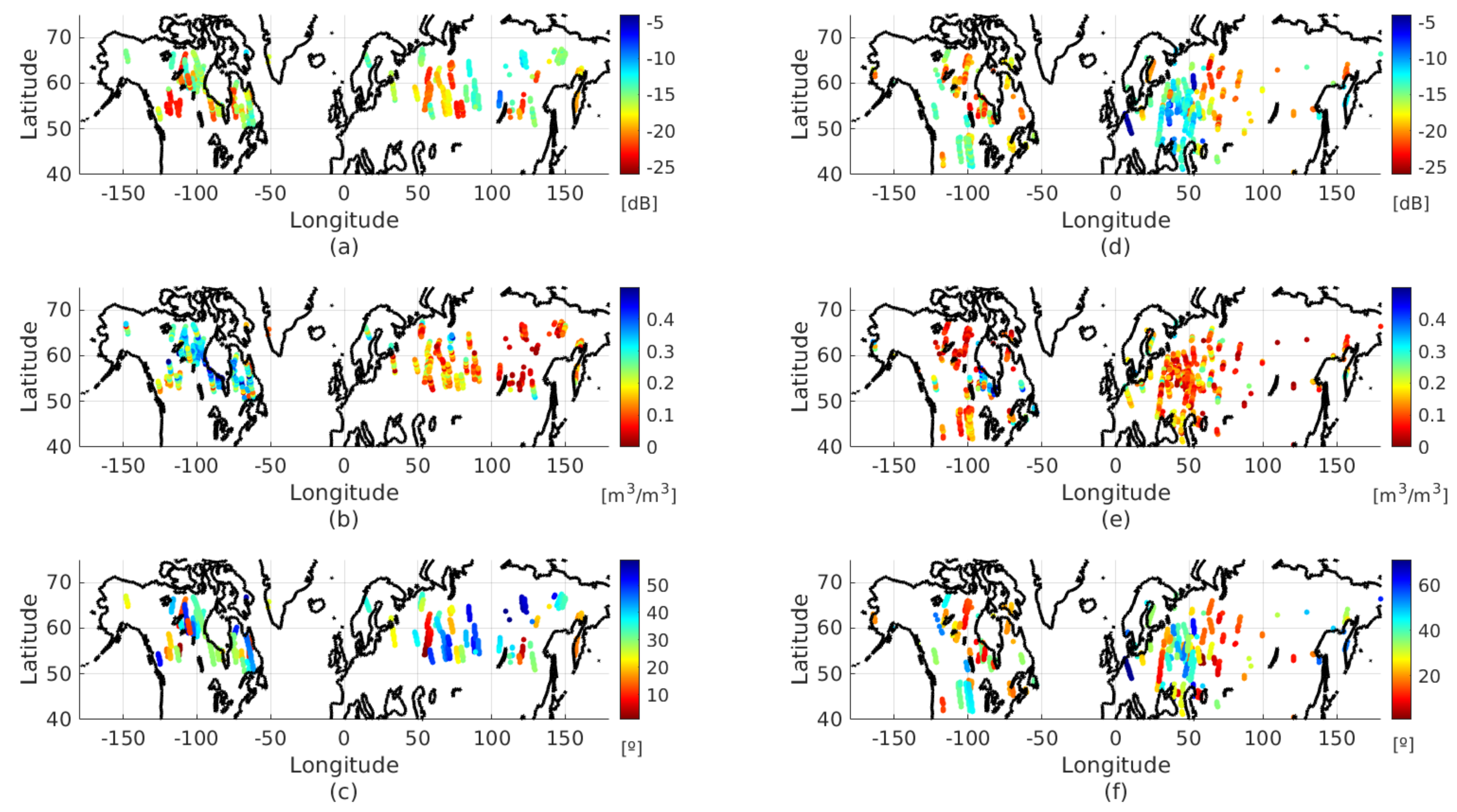
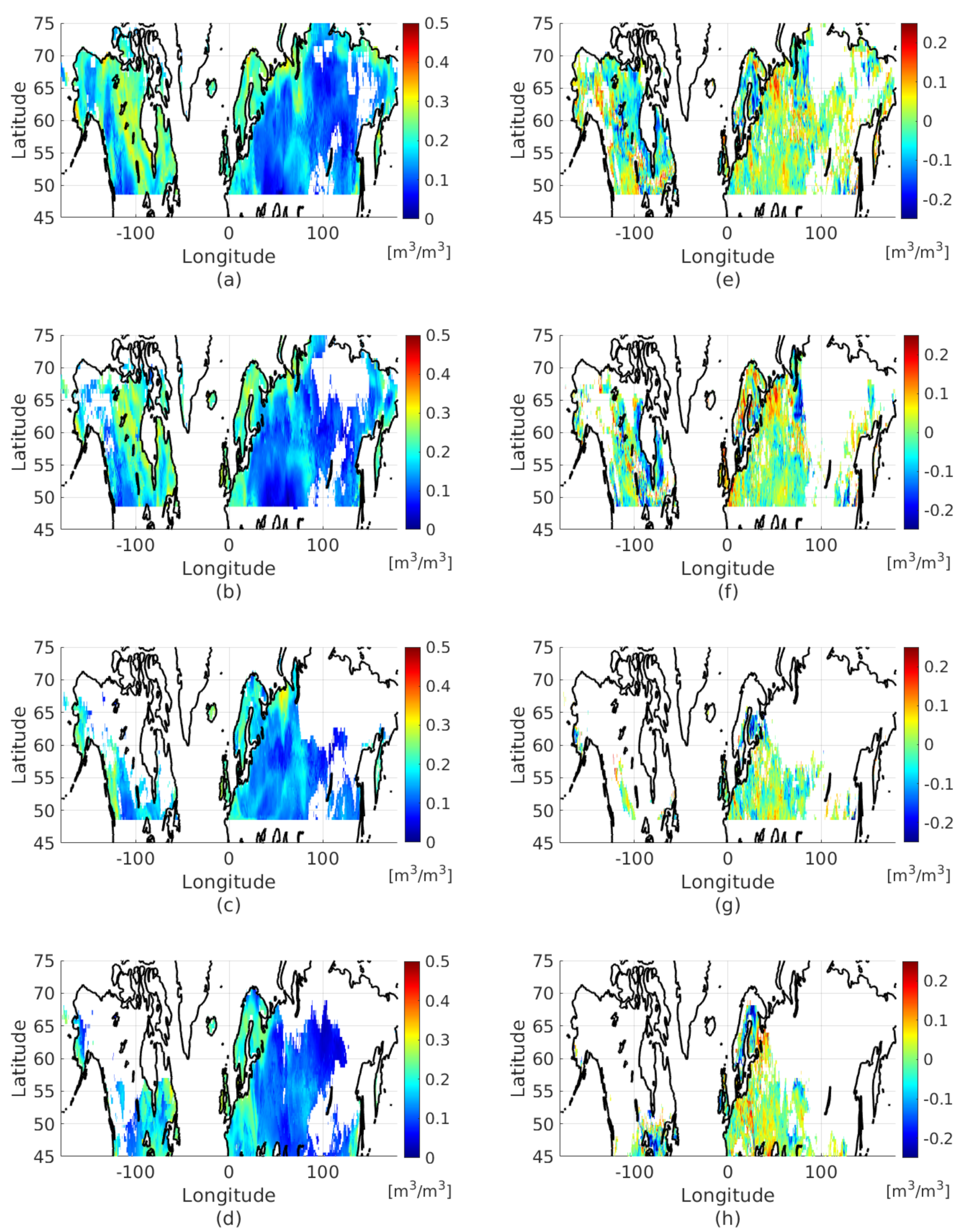
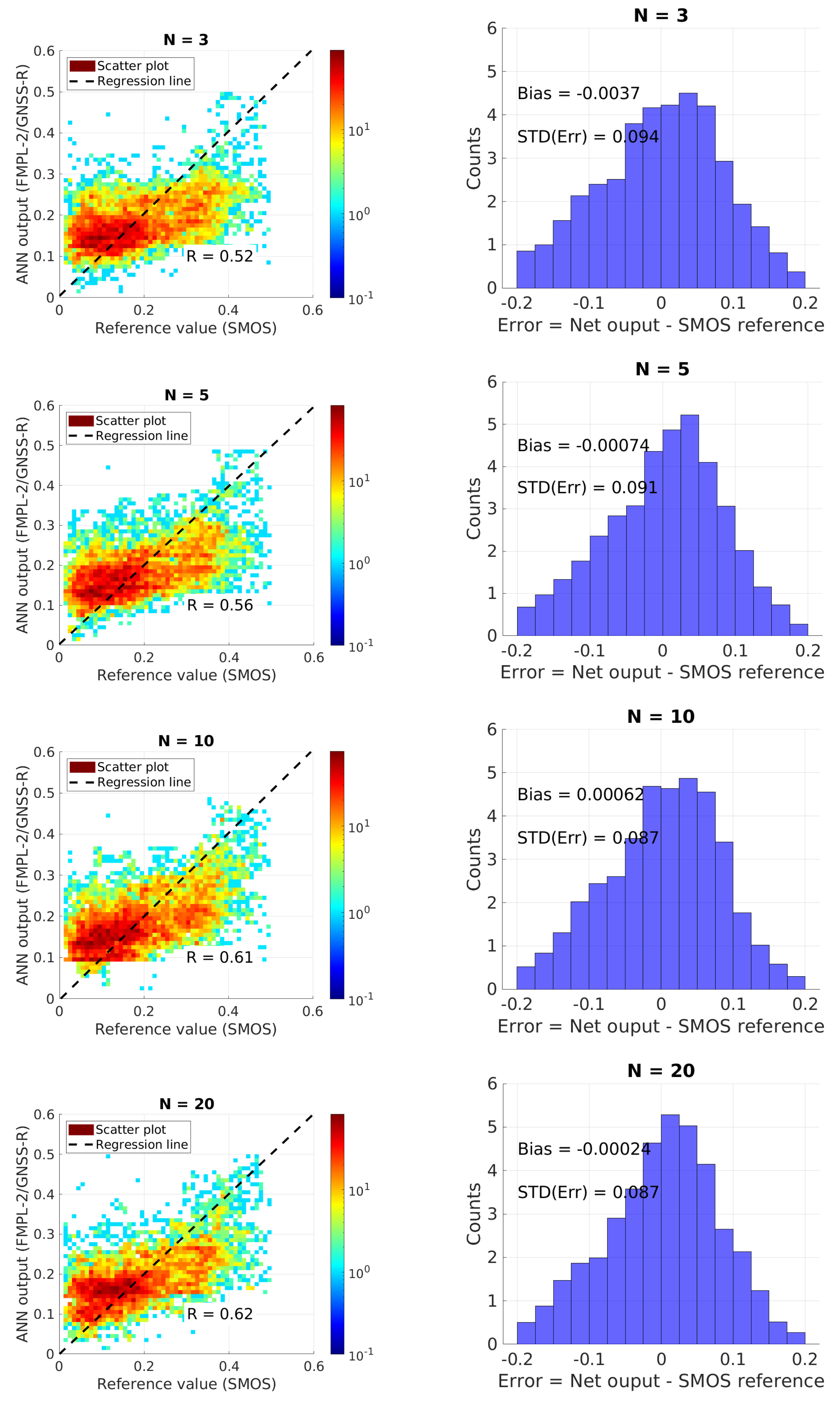
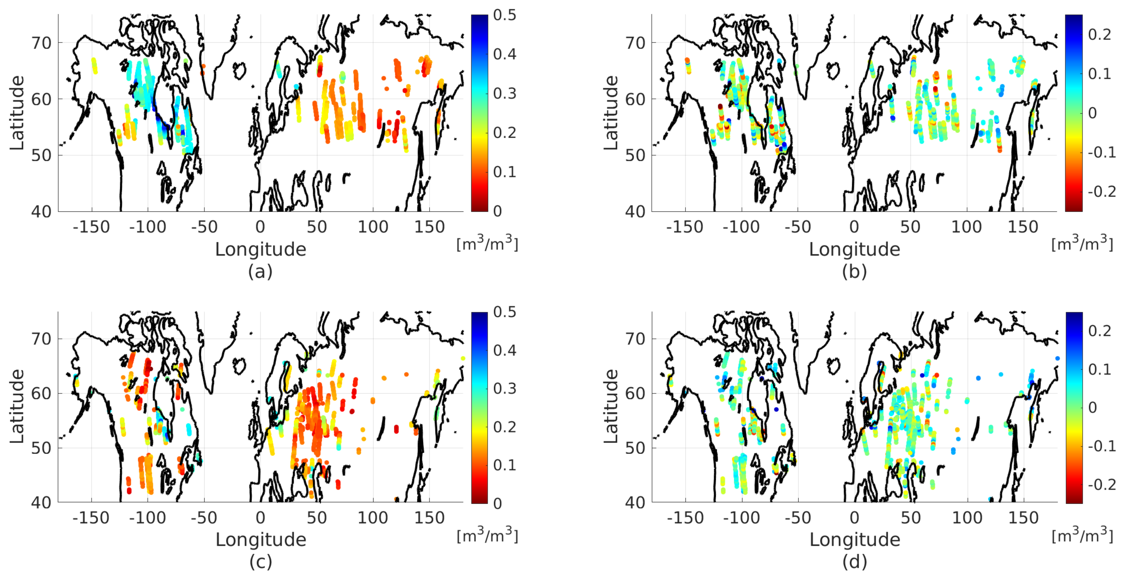
3.3. Using GNSS-R Data
- Incidence angle ,
- Moving average of the reflectivity (movmean()) over N samples,
- Moving standard deviation of the reflectivity (movstd()) over N samples, as a proxy to correct the surface roughness and speckle noise effects, and
- Moving average of the SNR (movmean(SNR)) over N samples.
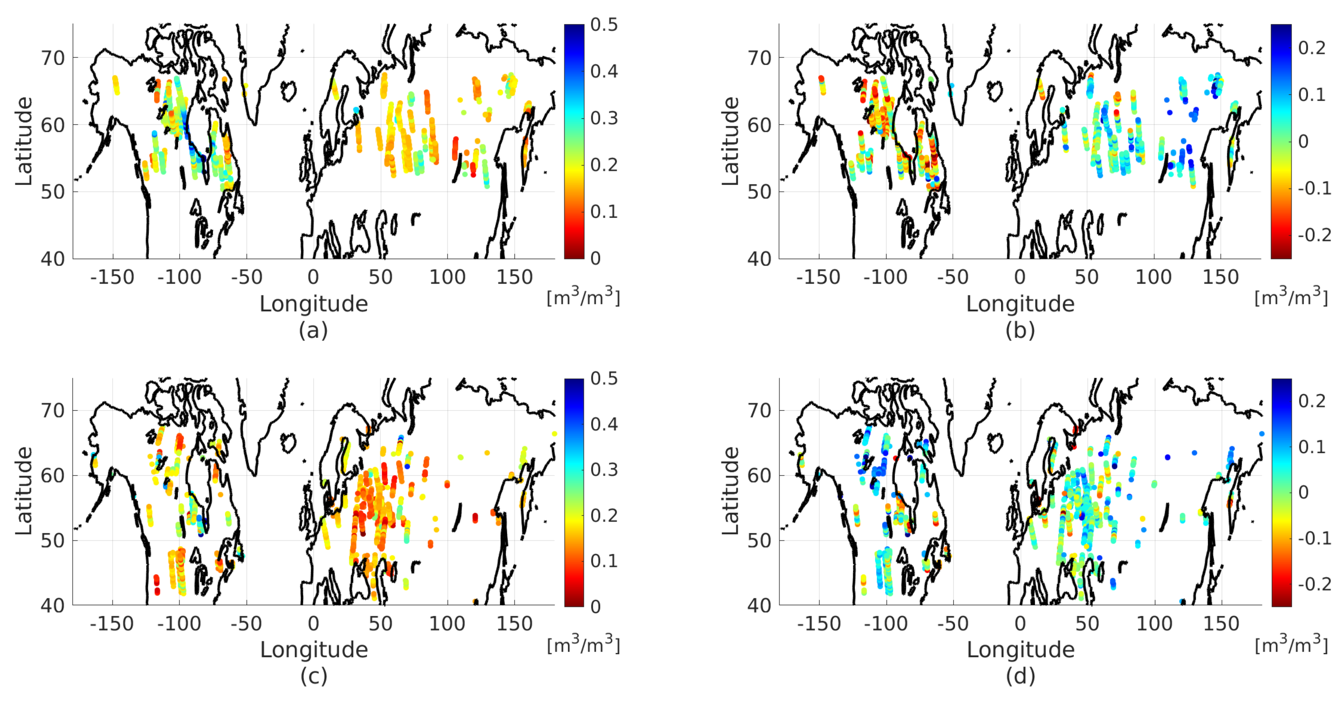
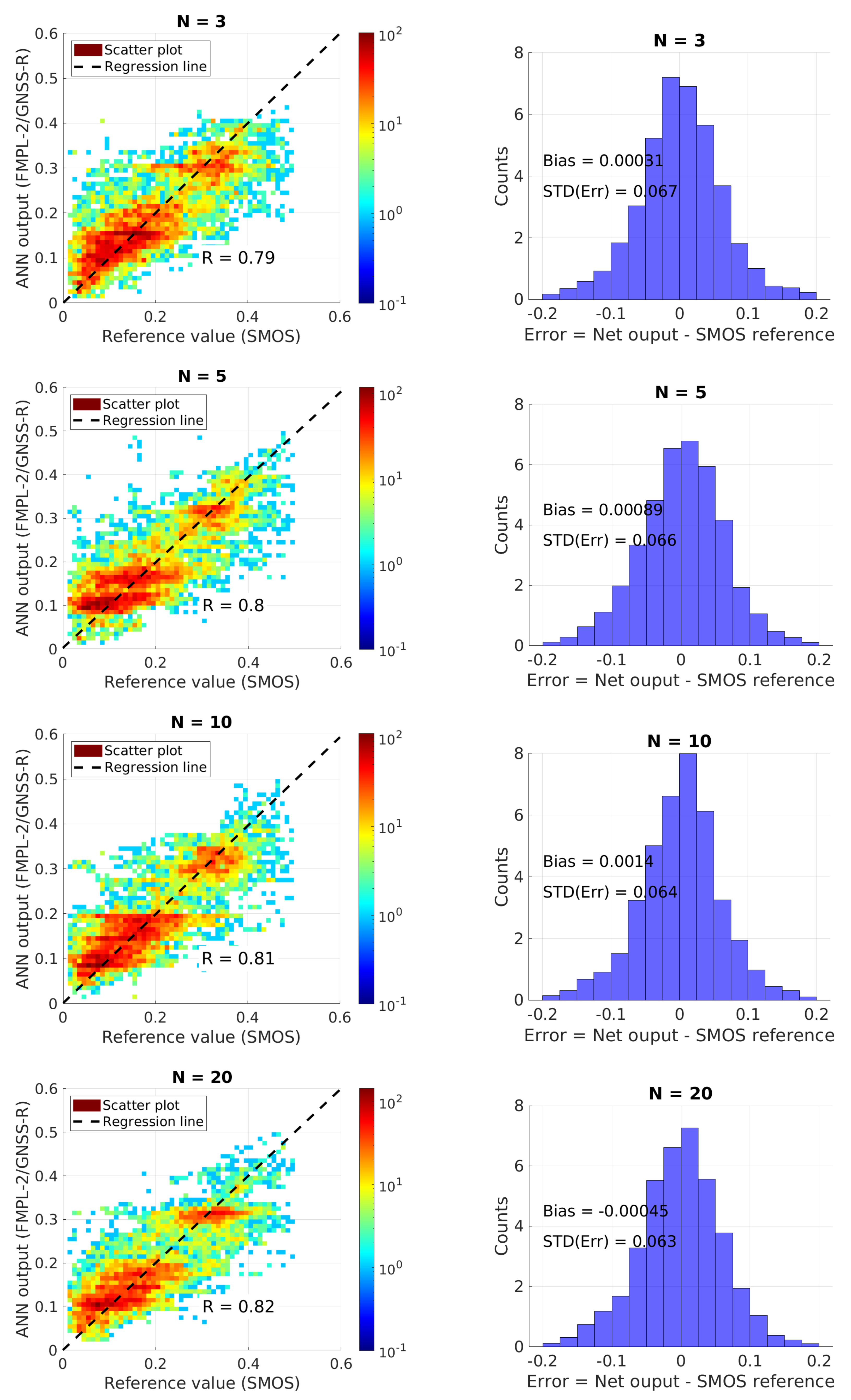
3.4. Using Combined GNSS-R and Radiometry Data
- FMPL-2 antenna temperature,
- FMPL-2 standard deviation of the antenna temperature in the along-track measurement,
- Incidence angle ,
- Moving average of the reflectivity (movmean()) over N samples,
- Moving standard deviation of the reflectivity (movstd()) over N samples, and
- Moving average of the SNR (movmean(SNR)) over N samples.
4. Discussion
5. Conclusions
Supplementary Materials
Author Contributions
Funding
Institutional Review Board Statement
Informed Consent Statement
Data Availability Statement
Acknowledgments
Conflicts of Interest
References
- GCOS. What are Essential Climate Variables? Available online: https://gcos.wmo.int/en/essential-climate-variables/abouth (accessed on 18 January 2021).
- Wasko, C.; Nathan, R. Influence of changes in rainfall and soil moisture on trends in flooding. J. Hydrol. 2019, 575, 432–441. [Google Scholar] [CrossRef]
- Wei, L.; Zhang, B.; Wang, M. Effects of antecedent soil moisture on runoff and soil erosion in alley cropping systems. Agric. Water Manag. 2007, 94, 54–62. [Google Scholar] [CrossRef]
- Miralles, D.G.; Gentine, P.; Seneviratne, S.I.; Teuling, A.J. Land-atmospheric feedbacks during droughts and heatwaves: State of the science and current challenges. Ann. N. Y. Acad. Sci. 2018, 1436, 19–35. [Google Scholar] [CrossRef]
- Badewa, E.; Unc, A.; Cheema, M.; Kavanagh, V.; Galagedara, L. Soil Moisture Mapping Using Multi-Frequency and Multi-Coil Electromagnetic Induction Sensors on Managed Podzols. Agronomy 2018, 8, 224. [Google Scholar] [CrossRef] [Green Version]
- Klotzsche, A.; Jonard, F.; Looms, M.; van der Kruk, J.; Huisman, J. Measuring Soil Water Content with Ground Penetrating Radar: A Decade of Progress. Vadose Zone J. 2018, 17, 180052. [Google Scholar] [CrossRef] [Green Version]
- Wu, K.; Rodriguez, G.A.; Zajc, M.; Jacquemin, E.; Clément, M.; Coster, A.D.; Lambot, S. A new drone-borne GPR for soil moisture mapping. Remote Sens. Environ. 2019, 235, 111456. [Google Scholar] [CrossRef]
- Petropoulos, G.P.; Ireland, G.; Barrett, B. Surface soil moisture retrievals from remote sensing: Current status, products & future trends. Phys. Chem. Earth Parts A/B/C 2015, 83–84, 36–56. [Google Scholar] [CrossRef]
- Jackson, R.D. Soil Moisture Inferences from Thermal-Infrared Measurements of Vegetation Temperatures. IEEE Trans. Geosci. Remote Sens. 1982, GE-20, 282–286. [Google Scholar] [CrossRef]
- Moran, M.; Clarke, T.; Inoue, Y.; Vidal, A. Estimating crop water deficit using the relation between surface-air temperature and spectral vegetation index. Remote Sens. Environ. 1994, 49, 246–263. [Google Scholar] [CrossRef]
- Rahimzadeh-Bajgiran, P.; Berg, A. Soil Moisture Retrievals Using Optical/TIR Methods. In Satellite Soil Moisture Retrieval; Elsevier: Amsterdam, The Netherlands, 2016; pp. 47–72. [Google Scholar] [CrossRef]
- Kerr, Y.H.; Waldteufel, P.; Wigneron, J.P.; Delwart, S.; Cabot, F.; Boutin, J.; Escorihuela, M.J.; Font, J.; Reul, N.; Gruhier, C.; et al. The SMOS Mission: New Tool for Monitoring Key Elements of the Global Water Cycle. Proc. IEEE 2010, 98, 666–687. [Google Scholar] [CrossRef] [Green Version]
- Entekhabi, D.; Njoku, E.G.; O’Neill, P.E.; Kellogg, K.H.; Crow, W.T.; Edelstein, W.N.; Entin, J.K.; Goodman, S.D.; Jackson, T.J.; Johnson, J.; et al. The Soil Moisture Active Passive (SMAP) Mission. Proc. IEEE 2010, 98, 704–716. [Google Scholar] [CrossRef]
- Naeimi, V.; Scipal, K.; Bartalis, Z.; Hasenauer, S.; Wagner, W. An Improved Soil Moisture Retrieval Algorithm for ERS and METOP Scatterometer Observations. IEEE Trans. Geosci. Remote Sens. 2009, 47, 1999–2013. [Google Scholar] [CrossRef]
- Hegarat-Mascle, S.L.; Zribi, M.; Alem, F.; Weisse, A.; Loumagne, C. Soil moisture estimation from ERS/SAR data: Toward an operational methodology. IEEE Trans. Geosci. Remote Sens. 2002, 40, 2647–2658. [Google Scholar] [CrossRef]
- Pathe, C.; Wagner, W.; Sabel, D.; Doubkova, M.; Basara, J.B. Using ENVISAT ASAR Global Mode Data for Surface Soil Moisture Retrieval Over Oklahoma, USA. IEEE Trans. Geosci. Remote Sens. 2009, 47, 468–480. [Google Scholar] [CrossRef]
- Srivastava, H.; Patel, P.; Sharma, Y.; Navalgund, R. Large-Area Soil Moisture Estimation Using Multi-Incidence-Angle RADARSAT-1 SAR Data. IEEE Trans. Geosci. Remote Sens. 2009, 47, 2528–2535. [Google Scholar] [CrossRef]
- Paloscia, S.; Pettinato, S.; Santi, E.; Notarnicola, C.; Pasolli, L.; Reppucci, A. Soil moisture mapping using Sentinel-1 images: Algorithm and preliminary validation. Remote Sens. Environ. 2013, 134, 234–248. [Google Scholar] [CrossRef]
- Gorrab, A.; Zribi, M.; Baghdadi, N.; Mougenot, B.; Fanise, P.; Chabaane, Z. Retrieval of Both Soil Moisture and Texture Using TerraSAR-X Images. Remote Sens. 2015, 7, 10098–10116. [Google Scholar] [CrossRef] [Green Version]
- Camps, A.; Vall·llossera, M.; Park, H.; Portal, G.; Rossato, L. Sensitivity of TDS-1 GNSS-R Reflectivity to Soil Moisture: Global and Regional Differences and Impact of Different Spatial Scales. Remote Sens. 2018, 10, 1856. [Google Scholar] [CrossRef] [Green Version]
- Chew, C.C.; Small, E.E. Soil Moisture Sensing Using Spaceborne GNSS Reflections: Comparison of CYGNSS Reflectivity to SMAP Soil Moisture. Geophys. Res. Lett. 2018, 45, 4049–4057. [Google Scholar] [CrossRef] [Green Version]
- Chew, C.; Small, E. Description of the UCAR/CU Soil Moisture Product. Remote Sens. 2020, 12, 1558. [Google Scholar] [CrossRef]
- Chew, C.; Shah, R.; Zuffada, C.; Hajj, G.; Masters, D.; Mannucci, A.J. Demonstrating soil moisture remote sensing with observations from the UK TechDemoSat-1 satellite mission. Geophys. Res. Lett. 2016, 43, 3317–3324. [Google Scholar] [CrossRef] [Green Version]
- Camps, A.; Park, H.; Pablos, M.; Foti, G.; Gommenginger, C.P.; Liu, P.; Judge, J. Sensitivity of GNSS-R Spaceborne Observations to Soil Moisture and Vegetation. IEEE J. Sel. Top. Appl. Earth Obs. Remote Sens. 2016, 9, 4730–4742. [Google Scholar] [CrossRef] [Green Version]
- Park, H.; Camps, A.; Castellvi, J.; Muro, J. Generic Performance Simulator of Spaceborne GNSS-Reflectometer for Land Applications. IEEE J. Sel. Top. Appl. Earth Obs. Remote Sens. 2020, 13, 3179–3191. [Google Scholar] [CrossRef]
- Camps, A.; Park, H.; Castellví, J.; Corbera, J.; Ascaso, E. Single-Pass Soil Moisture Retrievals Using GNSS-R: Lessons Learned. Remote Sens. 2020, 12, 2064. [Google Scholar] [CrossRef]
- Ruf, C.S.; Gleason, S.; Jelenak, Z.; Katzberg, S.; Ridley, A.; Rose, R.; Scherrer, J.; Zavorotny, V. The CYGNSS nanosatellite constellation hurricane mission. In Proceedings of the International Geoscience and Remote Sensing Symposium (IGARSS), Munich, Germany, 22–27 July 2012; pp. 214–216. [Google Scholar] [CrossRef]
- Unwin, M.; Jales, P.; Blunt, P.; Duncan, S.; Brummitt, M.; Ruf, C. The SGR-ReSI and its application for GNSS reflectometry on the NASA EV-2 CYGNSS mission. In Proceedings of the 2013 IEEE Aerospace Conference, Big Sky, MT, USA, 2–9 March 2013; pp. 1–6. [Google Scholar] [CrossRef]
- Yan, Q.; Huang, W.; Jin, S.; Jia, Y. Pan-tropical soil moisture mapping based on a three-layer model from CYGNSS GNSS-R data. Remote Sens. Environ. 2020, 247, 111944. [Google Scholar] [CrossRef]
- Senyurek, V.; Lei, F.; Boyd, D.; Kurum, M.; Gurbuz, A.C.; Moorhead, R. Machine Learning-Based CYGNSS Soil Moisture Estimates over ISMN sites in CONUS. Remote Sens. 2020, 12, 1168. [Google Scholar] [CrossRef] [Green Version]
- Clarizia, M.P.; Pierdicca, N.; Costantini, F.; Floury, N. Analysis of CYGNSS Data for Soil Moisture Retrieval. IEEE J. Sel. Top. Appl. Earth Obs. Remote Sens. 2019, 12, 2227–2235. [Google Scholar] [CrossRef]
- Al-Khaldi, M.M.; Johnson, J.T.; O’Brien, A.J.; Balenzano, A.; Mattia, F. Time-Series Retrieval of Soil Moisture Using CYGNSS. IEEE Trans. Geosci. Remote Sens. 2019, 57, 4322–4331. [Google Scholar] [CrossRef]
- Jing, C.; Niu, X.; Duan, C.; Lu, F.; Di, G.; Yang, X. Sea Surface Wind Speed Retrieval from the First Chinese GNSS-R Mission: Technique and Preliminary Results. Remote Sens. 2019, 11, 3013. [Google Scholar] [CrossRef] [Green Version]
- Jales, P.; Esterhuizen, S.; Masters, D.; Nguyen, V.; Correig, O.N.; Yuasa, T.; Cartwright, J. The new Spire GNSS-R satellite missions and products. In Image and Signal Processing for Remote Sensing XXVI; Bruzzone, L., Bovolo, F., Santi, E., Eds.; International Society for Optics and Photonics, SPIE: Washington, DC, USA, 2020; Volume 11533. [Google Scholar] [CrossRef]
- Camps, A.; Golkar, A.; Gutierrez, A.; de Azua, J.A.R.; Munoz-Martin, J.F.; Fernandez, L.; Diez, C.; Aguilella, A.; Briatore, S.; Akhtyamov, R.; et al. FSSCat, the 2017 Copernicus Masters’ “Esa Sentinel Small Satellite Challenge” Winner: A Federated Polar and Soil Moisture Tandem Mission Based on 6U Cubesats. In Proceedings of the IGARSS 2018—2018 IEEE International Geoscience and Remote Sensing Symposium, Valencia, Spain, 22–27 July 2018; pp. 8285–8287. [Google Scholar] [CrossRef]
- European Space Agency. Introducing the Newest ESA Third Party Missions. Available online: https://earth.esa.int/eogateway/news/introducing-the-newest-esa-third-party-missions (accessed on 8 January 2020).
- Munoz-Martin, J.F.; Fernandez-Capon, L.; Ruiz-de-Azua, J.; Camps, A. The Flexible Microwave Payload-2: A SDR-Based GNSS-Reflectometer and L-Band Radiometer for CubeSats. IEEE J. Sel. Top. Appl. Earth Obs. Remote Sens. 2020, 13, 1298–1311. [Google Scholar] [CrossRef]
- Munoz-Martin, J.F.; Fernandez, L.; Perez, A.; de Azua, J.A.R.; Park, H.; Camps, A.; Domínguez, B.C.; Pastena, M. In-Orbit Validation of the FMPL-2 Instrument—The GNSS-R and L-Band Microwave Radiometer Payload of the FSSCat Mission. Remote Sens. 2020, 13, 121. [Google Scholar] [CrossRef]
- Kerr, Y.; Al-Yaari, A.; Rodriguez-Fernandez, N.; Parrens, M.; Molero, B.; Leroux, D.; Bircher, S.; Mahmoodi, A.; Mialon, A.; Richaume, P.; et al. Overview of SMOS performance in terms of global soil moisture monitoring after six years in operation. Remote Sens. Environ. 2016, 180, 40–63. [Google Scholar] [CrossRef]
- Center, B.E. Barcelona Expert Center Webpage. Available online: Http://bec.icm.csic.es/ (accessed on 22 December 2020).
- Portal, G.; Vall-llossera, M.; Piles, M.; Camps, A.; Chaparro, D.; Pablos, M.; Rossato, L. A Spatially Consistent Downscaling Approach for SMOS Using an Adaptive Moving Window. IEEE J. Sel. Top. Appl. Earth Obs. Remote Sens. 2018, 11, 1883–1894. [Google Scholar] [CrossRef]
- Pablos, M.; Vall-llossera, M.; Piles, M.; Camps, A.; González-Haro, C.; Turiel, A.; Herbert, C.J.; Chaparro, D.; Portal, G. Influence of Quality Filtering Approaches in BEC SMOS L3 Soil Moisture Products. In Proceedings of the IGARSS 2019—2019 IEEE International Geoscience and Remote Sensing Symposium, Yokohama, Japan, 28 July–2 August 2019; pp. 6941–6944. [Google Scholar] [CrossRef]
- Pablos, M.; Piles, M.; Gonzalez-Haro, C. BEC SMOS Land Products Description. Available online: Http://bec.icm.csic.es/doc/BEC-SMOS-0003-PD-Land.pdf (accessed on 22 December 2020).
- Portal, G.; Jagdhuber, T.; Vall-llossera, M.; Camps, A.; Pablos, M.; Entekhabi, D.; Piles, M. Assessment of Multi-Scale SMOS and SMAP Soil Moisture Products across the Iberian Peninsula. Remote Sens. 2020, 12, 570. [Google Scholar] [CrossRef] [Green Version]
- Gherboudj, I.; Magagi, R.; Goita, K.; Berg, A.A.; Toth, B.; Walker, A. Validation of SMOS Data Over Agricultural and Boreal Forest Areas in Canada. IEEE Trans. Geosci. Remote Sens. 2012, 50, 1623–1635. [Google Scholar] [CrossRef]
- Bitar, A.A.; Leroux, D.; Kerr, Y.H.; Merlin, O.; Richaume, P.; Sahoo, A.; Wood, E.F. Evaluation of SMOS Soil Moisture Products Over Continental U.S. Using the SCAN/SNOTEL Network. IEEE Trans. Geosci. Remote Sens. 2012, 50, 1572–1586. [Google Scholar] [CrossRef] [Green Version]
- European Space Agency. Read-Me-First Note for the Release of the SMOS Level 2 Soil Moisture Data Products: Level 2 Soil Moisture V650; European Space Agency: Paris, France, 2017. [Google Scholar]
- Brodzik, M.J.; Billingsley, B.; Haran, T.; Raup, B.; Savoie, M.H. EASE-Grid 2.0: Incremental but Significant Improvements for Earth-Gridded Data Sets. ISPRS Int. J. Geo-Inf. 2012, 1, 32–45. [Google Scholar] [CrossRef] [Green Version]
- Didan, K. MOD13Q1 MODIS/Terra Vegetation Indices 16-Day L3 Global 250m SIN Grid V006, 2015. Available online: https://doi.org/10.5067/MODIS/MOD13Q1.006 (accessed on 1 November 2020).
- Owens, R.; Hewson, T. ECMWF Forecast User Guide 2018. Available online: https://doi.org/10.21957/M1CS7H (accessed on 1 November 2020). [CrossRef]
- European Space Agency. Eight Years of SMOS Arctic Sea Ice Thickness Level Now Available from SMOS Data Dissemination Portal. Available online: https://earth.esa.int/web/guest/missions/esa-operational-eo-missions/smos/news/-/article/eight-years-data-of-smos-arctic-sea-ice-thickness-level-now-available-from-smos-data-dissemination-portal (accessed on 11 November 2019).
- Rodriguez-Fernandez, N.J.; Aires, F.; Richaume, P.; Kerr, Y.H.; Prigent, C.; Kolassa, J.; Cabot, F.; Jimenez, C.; Mahmoodi, A.; Drusch, M. Soil Moisture Retrieval Using Neural Networks: Application to SMOS. IEEE Trans. Geosci. Remote Sens. 2015, 53, 5991–6007. [Google Scholar] [CrossRef]
- Eroglu, O.; Kurum, M.; Boyd, D.; Gurbuz, A.C. High Spatio-Temporal Resolution CYGNSS Soil Moisture Estimates Using Artificial Neural Networks. Remote Sens. 2019, 11, 2272. [Google Scholar] [CrossRef] [Green Version]
- Ying, X. An Overview of Overfitting and its Solutions. J. Phys. Conf. Ser. 2019, 1168, 022022. [Google Scholar] [CrossRef]
- Yan, Q.; Gong, S.; Jin, S.; Huang, W.; Zhang, C. Near Real-Time Soil Moisture in China Retrieved From CyGNSS Reflectivity. IEEE Geosci. Remote. Sens. Lett. 2020, 1–5. [Google Scholar] [CrossRef]
- Karnin, E.D. A simple procedure for pruning back-propagation trained neural networks. IEEE Trans. Neural Netw. 1990, 1, 239–242. [Google Scholar] [CrossRef] [PubMed]
- Piles, M.; Camps, A.; Vall-llossera, M.; Corbella, I.; Panciera, R.; Rüdiger, C.; Kerr, Y.H.; Walker, J. Downscaling SMOS-Derived Soil Moisture Using MODIS Visible/Infrared Data. IEEE Trans. Geosci. Remote Sens. 2011, 49, 3156–3166. [Google Scholar] [CrossRef]
- Hajj, M.E.; Baghdadi, N.; Zribi, M.; Rodríguez-Fernández, N.; Wigneron, J.; Al-Yaari, A.; Bitar, A.A.; Albergel, C.; Calvet, J.C. Evaluation of SMOS, SMAP, ASCAT and Sentinel-1 Soil Moisture Products at Sites in Southwestern France. Remote Sens. 2018, 10, 569. [Google Scholar] [CrossRef] [Green Version]
- Edokossi, K.; Calabia, A.; Jin, S.; Molina, I. GNSS-Reflectometry and Remote Sensing of Soil Moisture: A Review of Measurement Techniques, Methods, and Applications. Remote Sens. 2020, 12, 614. [Google Scholar] [CrossRef] [Green Version]
- Unwin, M. The SGR-ReSI Experiment on the TechDemoSat-1 Mission; Technical report; Surrey Satellite Technology Ltd.: Guildford, UK, 2015. [Google Scholar]
- Park, H.; Pascual, D.; Camps, A.; Martin, F.; Alonso-Arroyo, A.; Carreno-Luengo, H. Analysis of Spaceborne GNSS-R Delay-Doppler Tracking. IEEE J. Sel. Top. Appl. Earth Obs. Remote Sens. 2014, 7, 1481–1492. [Google Scholar] [CrossRef]
- Munoz-Martin, J.F.; Onrubia, R.; Pascual, D.; Park, H.; Camps, A.; Rüdiger, C.; Walker, J.; Monerris, A. Single-Pass Soil Moisture Retrieval Using GNSS-R at L1 and L5 Bands: Results from Airborne Experiment. Remote Sens. 2021, 13, 797. [Google Scholar] [CrossRef]
- Valencia, E.; Camps, A.; Vall-llossera, M.; Monerris, A.; Bosch-Lluis, X.; Rodriguez-Alvarez, N.; Ramos-Perez, I.; Marchan-Hernandez, J.F.; Martinez-Fernandez, J.; Sanchez-Martin, N.; et al. GNSS-R Delay-Doppler Maps over land: Preliminary results of the GRAJO field experiment. In Proceedings of the 2010 IEEE International Geoscience and Remote Sensing Symposium, Honolulu, HI, USA, 25–30 July 2010; pp. 3805–3808. [Google Scholar] [CrossRef]
- Emery, W.; Camps, A. Chapter 4-Microwave Radiometry. In Introduction to Satellite Remote Sensing; Elsevier: Amsterdam, The Netherlands, 2017; pp. 131–290. [Google Scholar] [CrossRef]
- Jiancheng, S.; Chen, K.S.; Qin, L.; Jackson, T.J.; O’Neill, P.E.; Leung, T. A parameterized surface reflectivity model and estimation of bare-surface soil moisture with L-band radiometer. IEEE Trans. Geosci. Remote Sens. 2002, 40, 2674–2686. [Google Scholar] [CrossRef]
- Onrubia, R.; Pascual, D.; Querol, J.; Park, H.; Camps, A. The Global Navigation Satellite Systems Reflectometry (GNSS-R) Microwave Interferometric Reflectometer: Hardware, Calibration, and Validation Experiments. Sensors 2019, 19, 1019. [Google Scholar] [CrossRef] [Green Version]


| Model | Input Data | Ground Truth |
|---|---|---|
| Optical |
| SMOS SM product at 36 km |
| Optical + MWR |
| SMOS SM product at 36 km |
| GNSS-R |
| SMOS SM product at 9 km |
| GNSS-R + MWR |
| SMOS SM product at 9 km |
| Model | R | Std(Err) (mm) | Bias (mm) |
|---|---|---|---|
| Optical | 0.56 | 0.084 | <10 |
| Optical + MWR | 0.69 | 0.074 | ~ |
| GNSS-R () | 0.62 | 0.087 | ~ |
| GNSS-R () + MWR | 0.82 | 0.063 | ~ |
Publisher’s Note: MDPI stays neutral with regard to jurisdictional claims in published maps and institutional affiliations. |
© 2021 by the authors. Licensee MDPI, Basel, Switzerland. This article is an open access article distributed under the terms and conditions of the Creative Commons Attribution (CC BY) license (http://creativecommons.org/licenses/by/4.0/).
Share and Cite
Munoz-Martin, J.F.; Llaveria, D.; Herbert, C.; Pablos, M.; Park, H.; Camps, A. Soil Moisture Estimation Synergy Using GNSS-R and L-Band Microwave Radiometry Data from FSSCat/FMPL-2. Remote Sens. 2021, 13, 994. https://doi.org/10.3390/rs13050994
Munoz-Martin JF, Llaveria D, Herbert C, Pablos M, Park H, Camps A. Soil Moisture Estimation Synergy Using GNSS-R and L-Band Microwave Radiometry Data from FSSCat/FMPL-2. Remote Sensing. 2021; 13(5):994. https://doi.org/10.3390/rs13050994
Chicago/Turabian StyleMunoz-Martin, Joan Francesc, David Llaveria, Christoph Herbert, Miriam Pablos, Hyuk Park, and Adriano Camps. 2021. "Soil Moisture Estimation Synergy Using GNSS-R and L-Band Microwave Radiometry Data from FSSCat/FMPL-2" Remote Sensing 13, no. 5: 994. https://doi.org/10.3390/rs13050994