
Using Geophysics to Characterize a Prehistoric Burial Mound in Romania
by
 , and
, and
Alexandru Hegyi
1,*, 
Dragoș Diaconescu
2,
Petru Urdea
1,
Apostolos Sarris
3,
Michał Pisz
4 and
Alexandru Onaca
1 1
Applied Geomorphology and Interdisciplinary Research Centre (CGACI), Department of Geography, West University of Timișoara, 300223 Timișoara, Timis, Romania
2
National Banat Museum of Timișoara, 300054 Timișoara, Timis, Romania
3
Sylvia Ioannou Chair in Digital Humanities, Archaeological Research Unit, Department of History and Archaeology, University of Cyprus, 1095 Nicosia, Cyprus
4
Institute of Hydrogeology and Geological Engineering, Faculty of Geology, University of Warsaw, 02-089 Warsaw, Poland
*
Author to whom correspondence should be addressed.
Remote Sens. 2021, 13(5), 842; https://doi.org/10.3390/rs13050842
Submission received: 6 January 2021
/
Revised: 15 February 2021
/
Accepted: 18 February 2021
/
Published: 24 February 2021
(This article belongs to the Special Issue Signal and Image Processing for Remote Sensing)
Abstract
:A geophysical investigation was carried across the M3 burial mound from Silvașu de Jos —Dealu Țapului, a tumuli necropolis in western Romania, where the presence of the Yamnaya people was certified archaeologically. For characterizing the inner structure of the mound, two conventional geophysical methods have been used: a geomagnetic survey and electrical resistivity tomography (ERT). The results allowed the mapping of the central features of the mound and the establishment of the relative stratigraphy of the mantle, which indicated at least two chronological phases. Archaeological excavations performed in the central part of the mound accurately validated the non-invasive geophysical survey and offered a valuable chronological record of the long-forgotten archaeological monument. Geophysical approaches proved to be an invaluable instrument for the exploration of the monument and suggest a fast constructive tool for the investigation of the entire necropolis which currently has a number of distinct mounds.
Keywords:
Yamnaya; tumuli; geophysics; geomagnetic survey; ERT; archaeology; archaeological prospection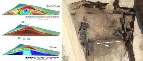
1. Introduction
Burial mounds, also called kurgans, barrows, or tumuli, are some of the most common examples of funerary archaeological objects. If preserved, they are usually easy to identify, due to their characteristic landform. Depending on the chronology and location, burial mounds could have different sizes and construction, from other smaller earthen mounds or large anthropogenic hills, highly distinctive in the present-day landscapes [1,2,3].
State-of-the-art remote sensing techniques and image processing methods allow researchers to locate, record, and analyze not only the presence of a burial mound but also its shape and size, even if they are located in a forest or other remote areas [4,5,6,7]. The challenging part starts when there is a need to determine the construction and the interior of the burial mound. Near-surface geophysics methods have been widely applied to this kind of archaeological feature over years. For example, magnetometry has proven its great value in both delineation and characterization of the burial mounds. Features detectable with magnetometry are usually the remains of pits and ditches, however, some inner structures and burial chambers might be magnetically contrasting with the parent rock as well [8,9,10]. Electrical geophysical methods are worldwide applied on burial mounds; however, they are mostly used in the case of bigger tumuli, to recognize their construction and internal structure. Appropriately applied electrical resistivity tomography (ERT) measurements might provide detailed 2D geoelectrical sections or even a 3D delineation of buried features [11,12,13]. Ground-penetrating radar is also increasingly applied in the course of burial mounds’ investigations [14,15,16,17,18].
1.1. Geographical Background
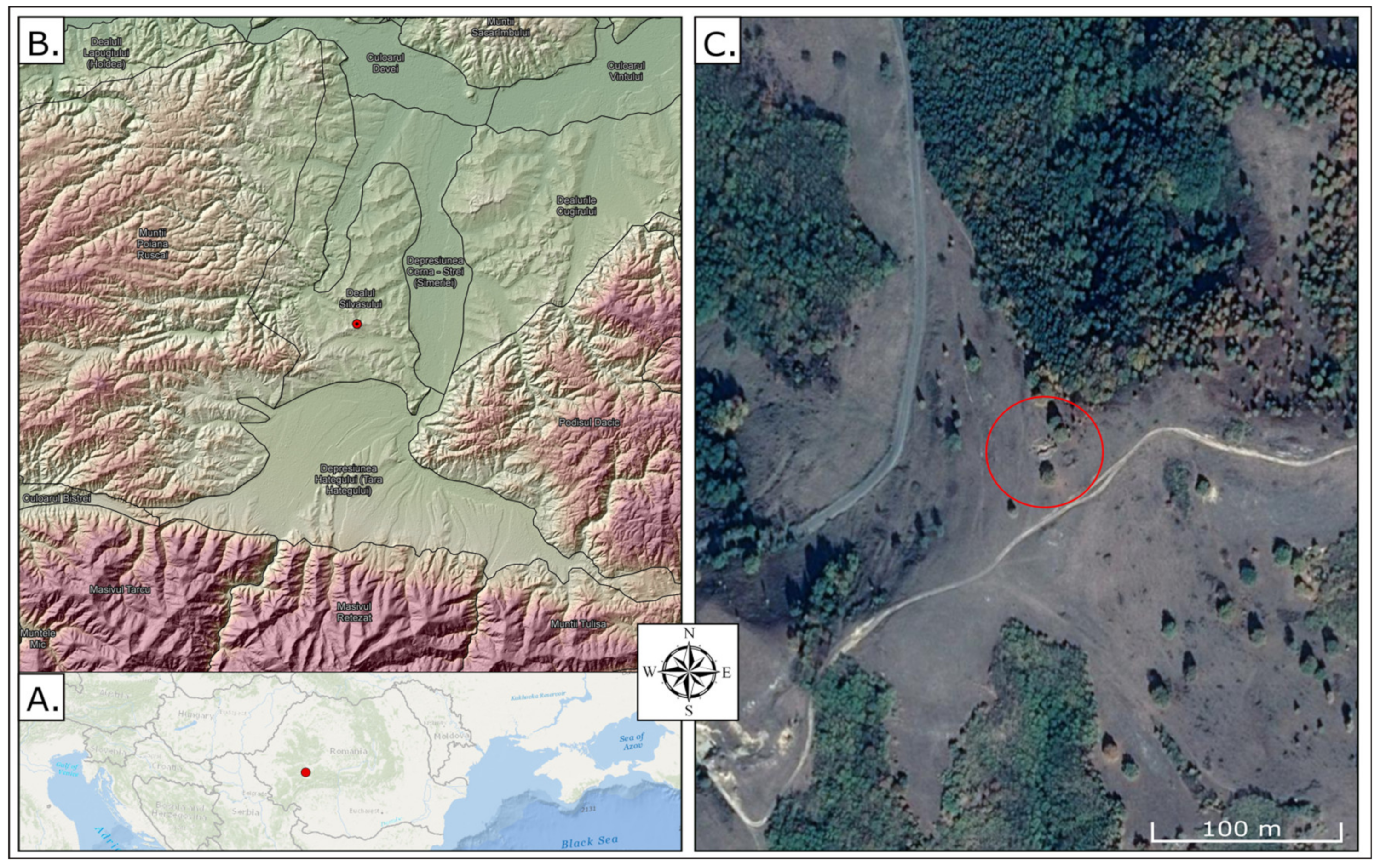
The natural setting of the archaeological site Silvașu de Jos-Dealu Țapului is situated in the Silvaşului Hills (Figure 1), a distinct southern part of the Hunedoara Hills, Romania, with a geomorphological landscape dominated by hills with wide and/or rounded interfluves with generally smooth slopes [19], and altitudes ranging between 300 to 400 m, reaching 527 m a.s.l. where mound M3 is located. The site is located in a geomorphological triplex continuum consisting of the watershed between the Cinciş river basins in the NW, the Moruzului Valley basin in the NE, and the Slivuț river basin in the south, all located in the Mures hydrographic basin, the most important river of Transylvania.
From a geological point of view, the territory belongs to the Haţeg-Strei Depression described by the presence of Neogene sedimentary formations. The stratigraphic succession, arranged in horizontal layers or slightly inclined (5°) to the NNE, is based on gravels, quarzitic oligomictic conglomerates, sands, reddish sandstones, and red marly clays of the Lower Miocene age over which are present, discordant deposits through badenian, gravels, sands, clays, and volcanic tuffs [20].
The presence of clays and marly clays horizons favors the appearance and development of landslides, even at the north-western slope located below the archaeological site. The rest slopes are smoother but still affected by weak rain wash erosion in grassland conditions. Only a few hundred meters to the NW of the site, an old and wide landslide is marked by a wavy relief with small depressions, some occupied by small lakes, designated as “La Tău”—“At the Lake” (popular “tău”, from “tó” Hungarian—lake).
1.2. Archaeological Background
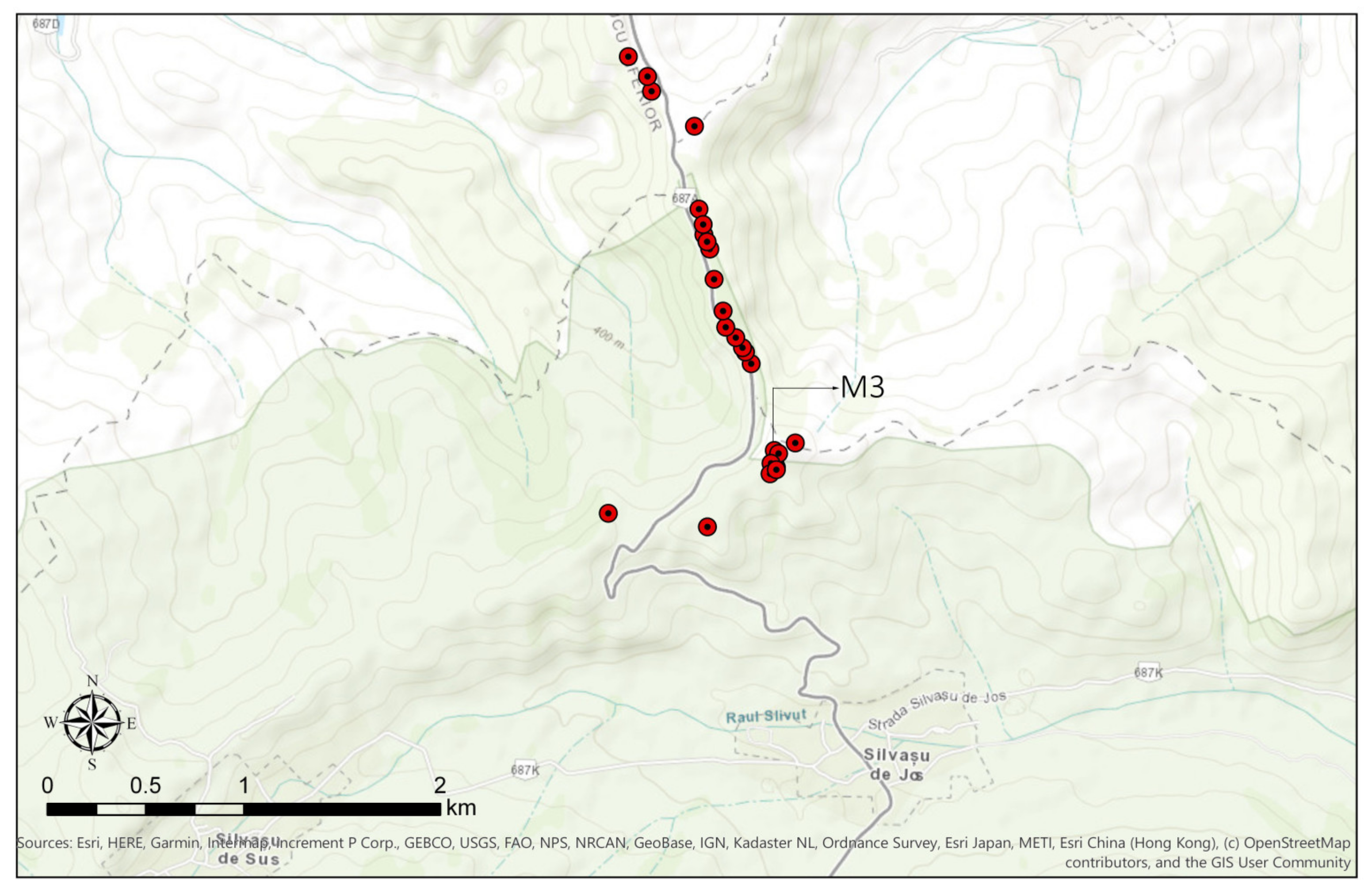
Of the 26 distinct mounds were found in the area (Figure 2), only four of them (M1, M3, M4, and M7) have been archaeologically investigated [21,22,23,24], which provided additional evidence of the stratigraphy and internal archaeological structures [22,24]. There are several distinct stages and elements in the construction process of each mound. Stratigraphically, there are several similarities, which can explain the chronological relationship between them. On the other hand, the stratigraphic similarities that were macroscopically noticed and underlined by Luca et al. 2011 [22] were contradicted by Diaconescu-Tincu 2016 [23] and Diaconescu 2020 [24] based on the Harris matrix analysis performed for the stratigraphic sequence of each excavated mound. A major similarity refers to the existence of the central feature: a pit that served to deposit the deceased, an element found in the case of mounds M3 and M4 [23]. The only difference is that in the case of mound M4, the inhumation grave was the primary one for the whole mound, while in mound M3, the inhumation grave can be considered as a primary one only for the second phase of construction of the mound [24].
The archaeological material collected during the research campaigns (Figure 3 and Figure 4) is composed mainly of ceramic vessels belonging to Cotofeni Culture (Late Eneolithic) having different stages of conservation. The absolute chronology of the necropolis was established by taking charcoal and osteological samples to produce an absolute chronology throughout 14C analyses. The bones were human, in the case of the skeleton found at M4, further analyses were performed with 13C and 13O isotopes (connected to the paleo-diet) [24]. Thus, so far, nine absolute dating samples (AMS) have been performed [24], which allowed the observation of two distinct chronological phases, the first corresponding to 3322–3062 cal BC (Coțofeni culture, phase IIIb) and the second to 2810–2642 cal BC, the last period corresponding to the chronology of the burial graves [23,24]. These two chronological phases were also observed stratigraphically (in the case of mound M3). The former estimates of the Bayesian model built for this necropolis originated from the stratigraphic observations done especially in mound M3 [24].
The archaeological research project conducted in the tumuli cemetery of Silvașu de Jos-Dealu Țapului underlined two very important aspects:
- The fashion of building funerary mounds started in Transylvania during Late Eneolithic (in Romanian archaeological literature also called the transition period between Eneolithic and Bronze Age), more precisely during the third phase of the Coțofeni culture (the mean value of the bounded sum for this stage, based on four 14C data, is ca. 3240 cal BC) and is connected to cremation burials and construction and burning of pyres/structures made of wooden beams. These conditions were identified in the mounds M1 and M3.
- The second stage of Silvașu de Jos cemetery is connected to Yamnaya culture/ Yamnaya cultural influences. During the XXth century in Transylvania and Romanian Banat, six prehistoric graves from Cîmpia Turzii, Cipău, Răscruci, Sânicolau Mare, Bodo, were attributed to the Ochre Grave Culture (i.e., Yamnaya culture). In Transylvania, menhirs of Nataljevka types were also discovered at Baia de Criș or Florești-Polus, representing funerary stelae connected with the North Pontic regions. In the case of Silvașu de Jos, it is clear that we are dealing with inhumation graves arranged in funerary mounds using timber elements, in oval or rectangular pits (found inside mounds M4 and M3 respectively). In the case of M3, it is obvious that the second stage of the mound was reused to arrange respectively the inhumation grave, increasing thus the barrow height. The mean value of the bounded sum for this stage of construction, based on five 14C data, is ca. 2720 cal BC.
2. Materials and Methods
The geophysical investigations focused on the M3 mound, which was later archaeologically investigated by Dr. Dragoș Diaconescu from the National Museum of Banat Timişoara, in five subsequent periods: 2015, 2016, 2017, 2019, and 2020.
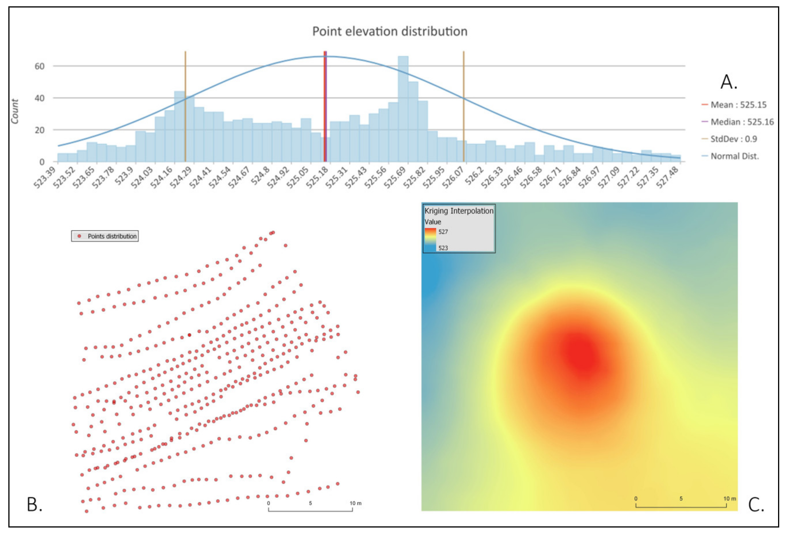
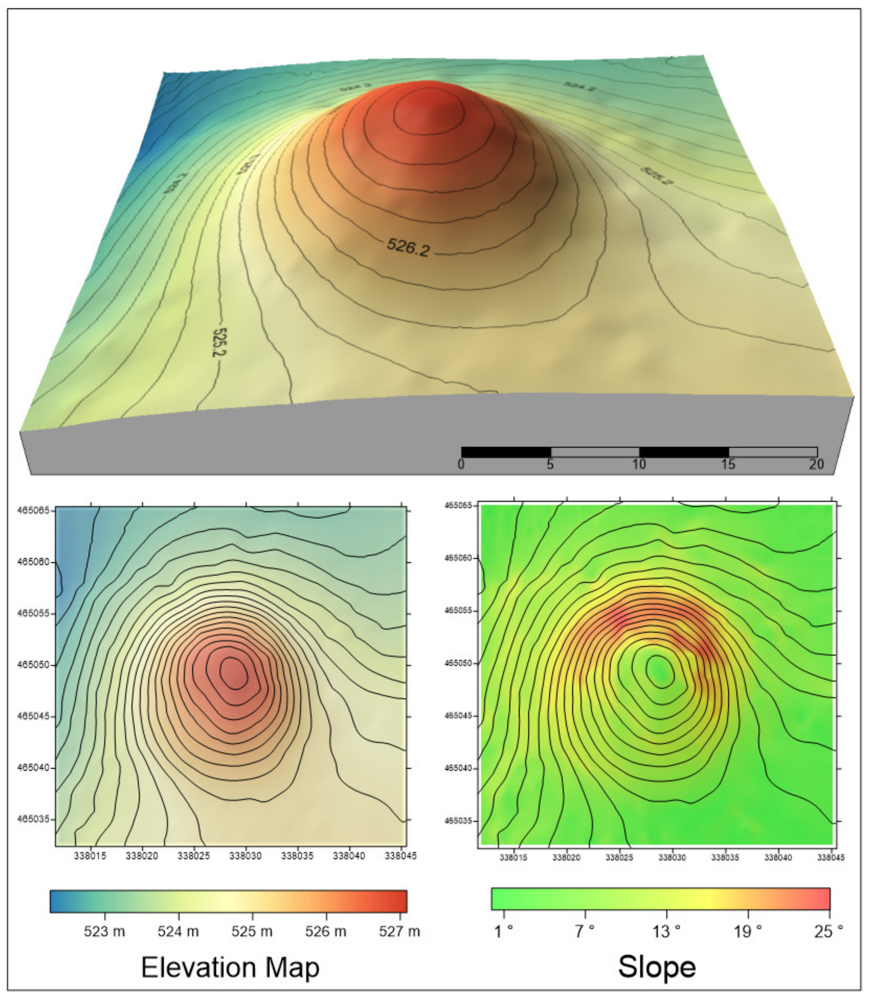
Initially, a detailed digital elevation model (DEM) was created by collecting 448 points (Figure 5B) with an RTK GNSS (TopCon Hiper V). The elevation points (Figure 5A) were interpolated (Figure 5C) in ArcGIS Pro using the Ordinary Kriging method with a spherical semi-variogram model and a lag size of 0.132. The model was rendered in Surfer 11. The slope and aspect were also calculated in ArcGIS Pro.
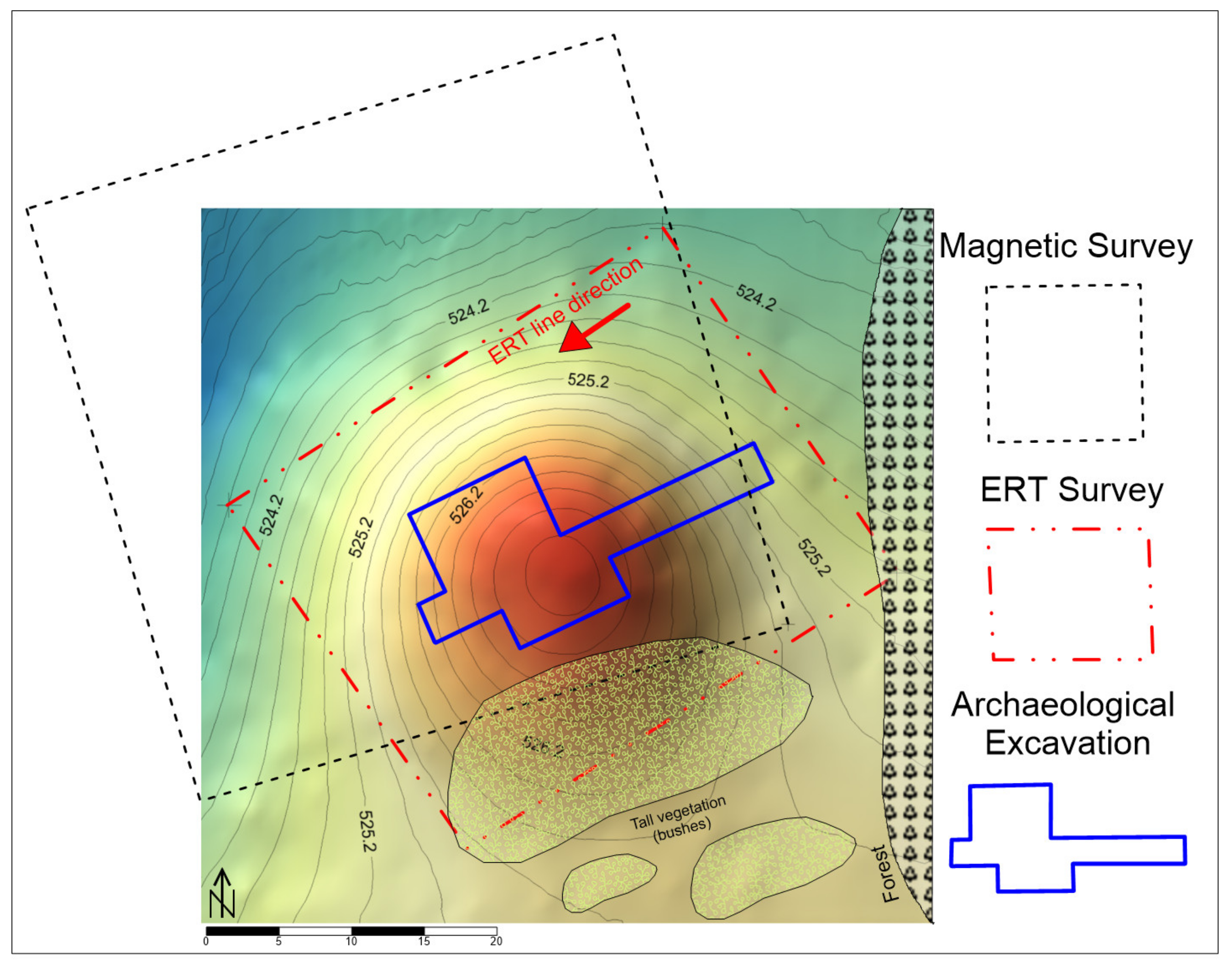
In the case of the M3 mound, two complementary geophysical methods (Figure 6) were used: a passive one taking geomagnetic measurements and an active one taking geoelectric measurements (electrical resistivity tomography/ERT).
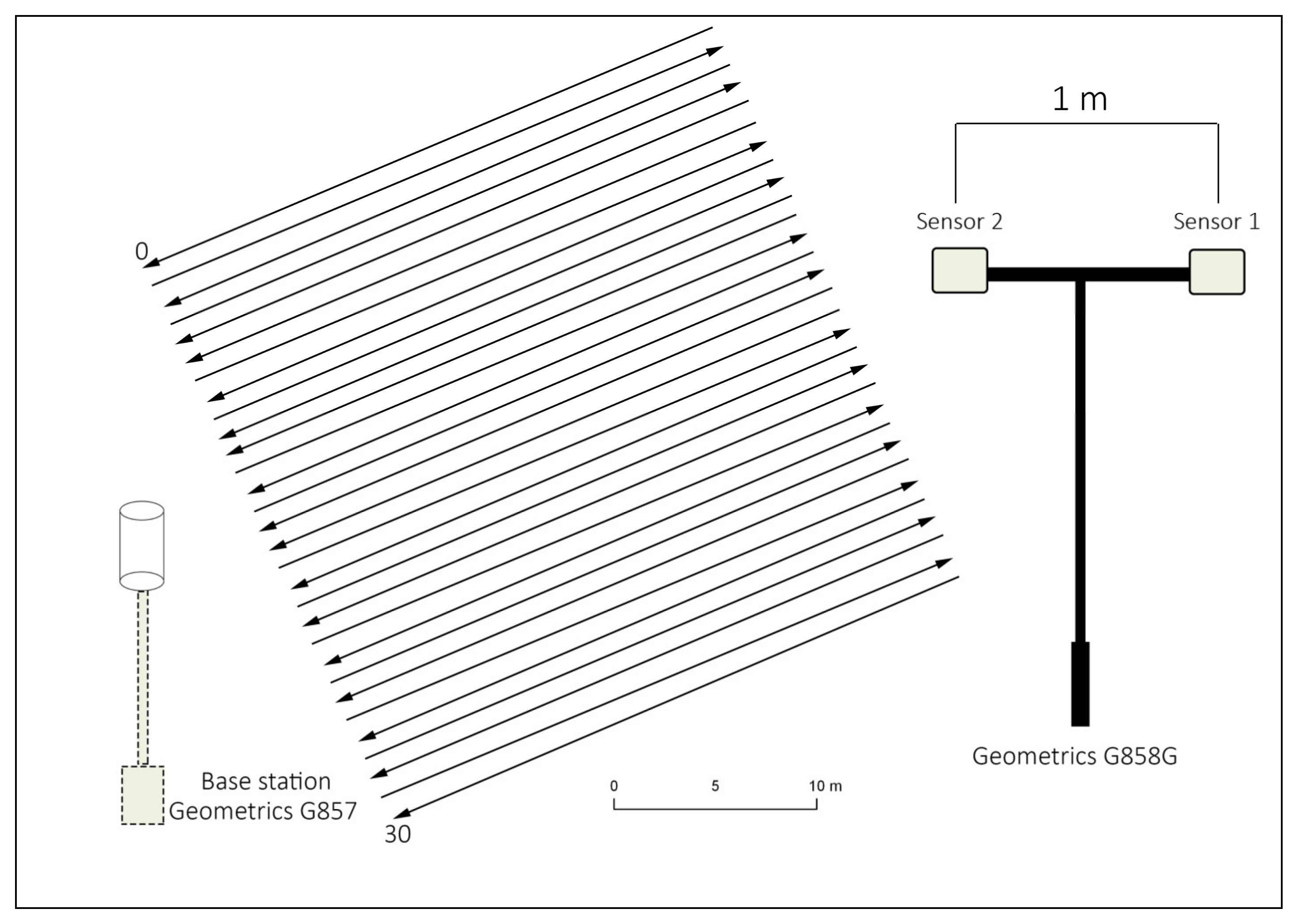
The geomagnetic measurements were obtained within a 30 m rectangle, along with parallel profiles 1 m apart (Figure 7). Samples were collected using two sensors Geometrics G858G cesium vapor precession magnetometer. The two sensors were set in a horizontal configuration. Each sensor measured 1 line. Therefore, 60 profiles were produced. A Geometrics G857 proton precession magnetometer was used as a correction base to reduce the impact of rapid magnetic variations. The dataset was processed in MagMap, MagPick, TerraSurveyor, and plotted in Surfer. Zero-Mean Travers and DeSlope functions were used. For better visualization of value distribution, a low-pass filter was overlaid.
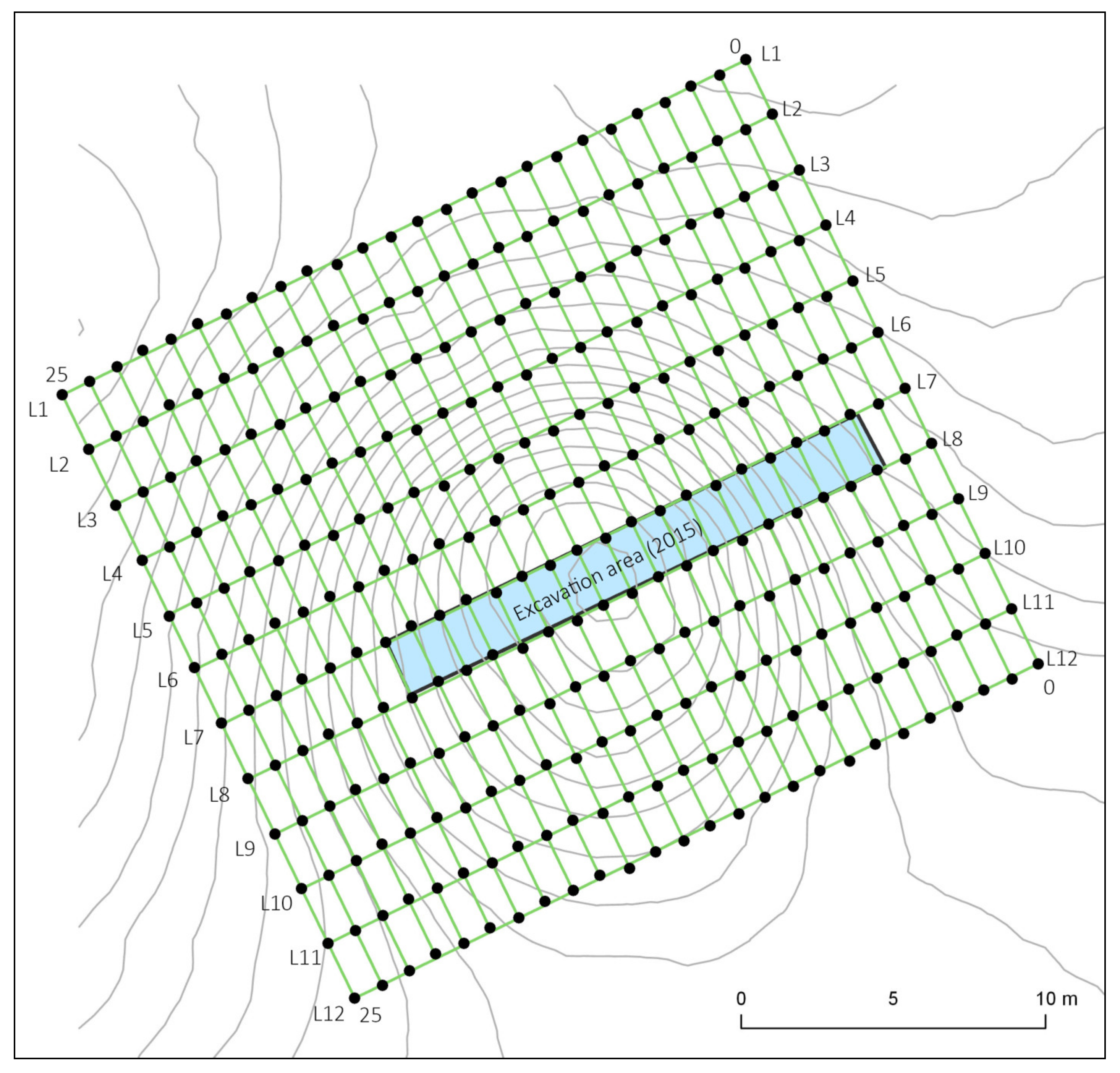
A GeoTom MK8E1000 high-resolution multi-electrode system was employed to carry out the geoelectric measurements, which were performed along 13 parallel profiles, 2 m apart, oriented in an NW-SE direction. The electrodes were arranged collinearly at 1 m spacing along with the profiles (Figure 8). Considering the local geology, Wenner, and Dipole–Dipole configurations were considered for performing the measurement. Each profile was inverted in Res2Dinv using a non-linear smoothness-constrained least-squares algorithm (Abs. error ranging between 3.2% to 5.5%). The topography of the mound was considered in the inversion process. The 3D modeling of resistivity values was performed in Res3Dinv (RMS Error 13.3%) and plotted in Voxler.
3. Results
3.1. Morphometrical Parameters
Understanding the morphology of the terrain and the morphometry of each mound is extremely important in preparing geophysical research. Based on the elevation model, it was possible to determine some morphometric characteristics of the mound, the most important referring to its elevation and slope (Figure 9).
The M3 mound has a diameter of 25 m, with a relatively circular base, and a maximum height of 2 m (Figure 2). The slope is more accentuated to the north, a consequence of the zonal relief, with the mound being located right on the southern edge of the interfluve. The northern part of the mound has a slope between 15 and 19 degrees, which caused a more pronounced erosion effect of the mantle towards the NNW, but also towards the NNE (Figure 9).
3.2. Geomagnetic Survey
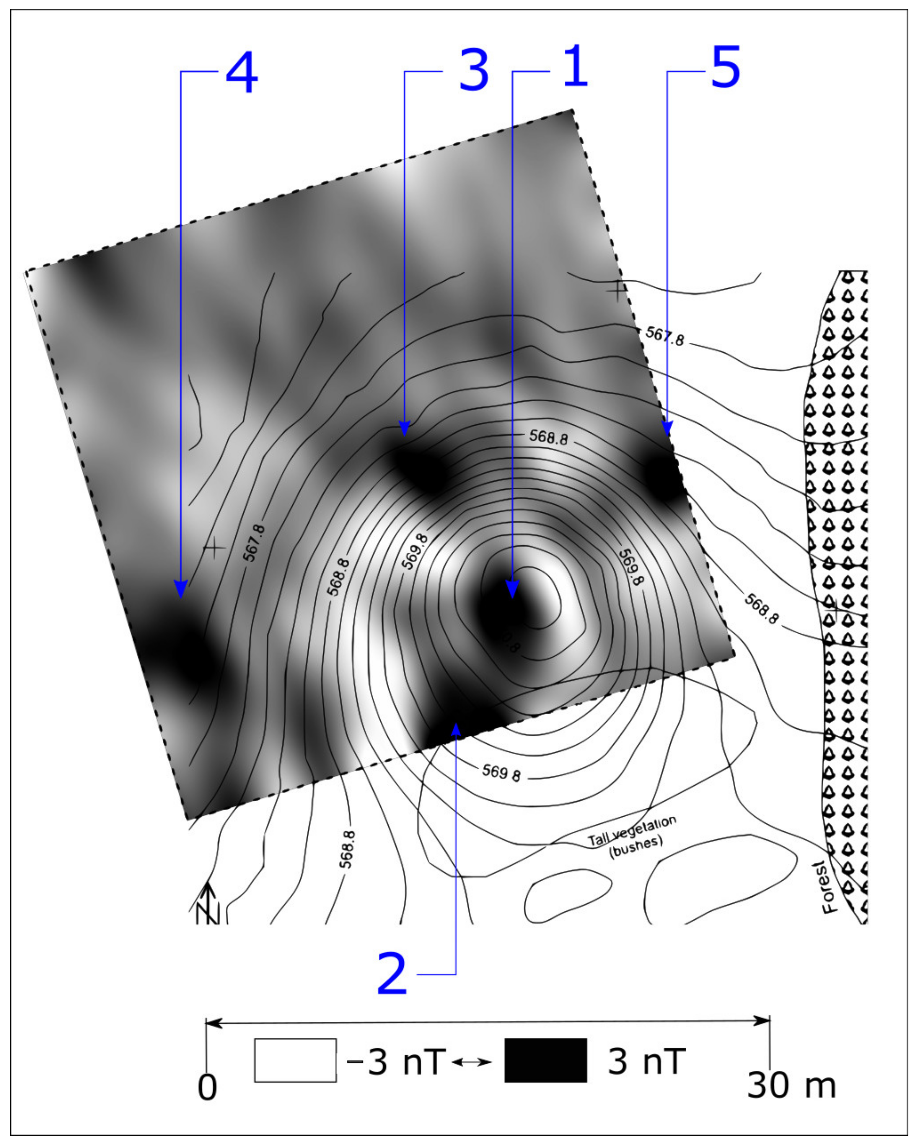
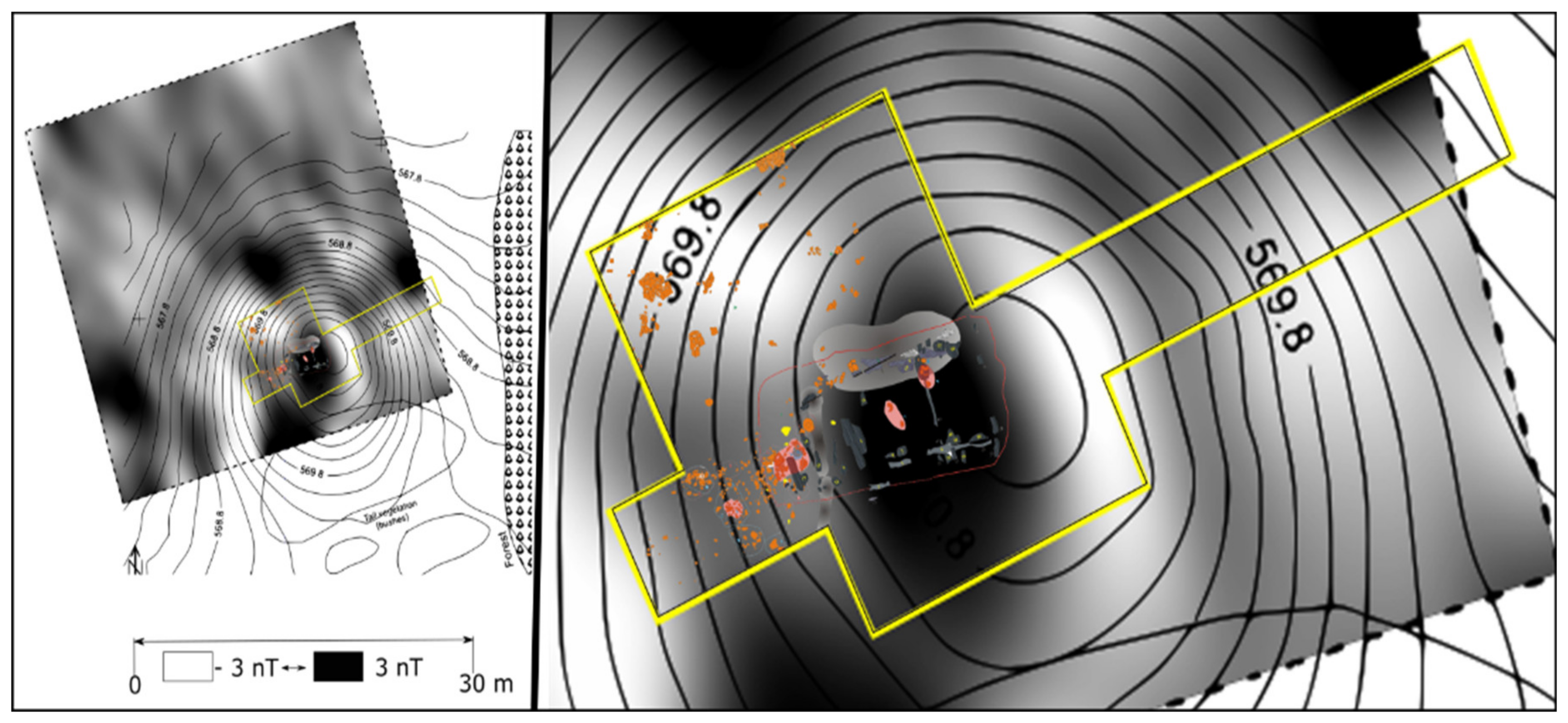
Five intense positive magnetic anomalies are distinguished on the top and at the vicinity of the mound (Figure 10). The positive anomalies (1–5) correspond to the various pits, some of which may be related to grave-pits. The distribution of the magnetic anomalies suggests a longer use of the mound and, as subsequent archaeological excavations have shown, the mound has several phases of existence.
However, from an archaeological point of view, the key points that explain the appearance of the mound are represented by anomalies 1 and probably 2. Anomaly 1 is located at the center of the mound and it may be considered as being the central feature around which the mound was built. Anomalies 2 and 3 are part of the whole central complex and suggest a more multifaceted anthropogenic intervention inside the mound. These features can appear due to the deposition of ceramic materials together with the cremated remains of the deceased, but they can also represent "in situ" incineration pits or grave pits. Anomalies 4 and 5 seem somehow displaced from the initial context of the mound, being positioned towards the boundaries of the mound. This observation leads us to believe that the two anomalies correspond to subsequent pits (maybe grave pits) in the mantle or outside the mound.
Even if the field conditions for collecting magnetic data were not ideal, the very small intensity of the magnetic values, blurred by the relatively thick layer of clay that constitutes the mantle, provided sufficient information to outline the location of the archaeological features inside the M3 mound.
3.3. Electrical Resistivity Tomography (ERT) Survey
The use of electrical resistivity tomography (ERT) was intended to capture the stratigraphic sequences of the M3 mound and enrich the information content of the archaeological features highlighted by the geomagnetic measurements. Thus, based on the profiles interpolation, a 2.5 D model of the underground resistivity was generated.
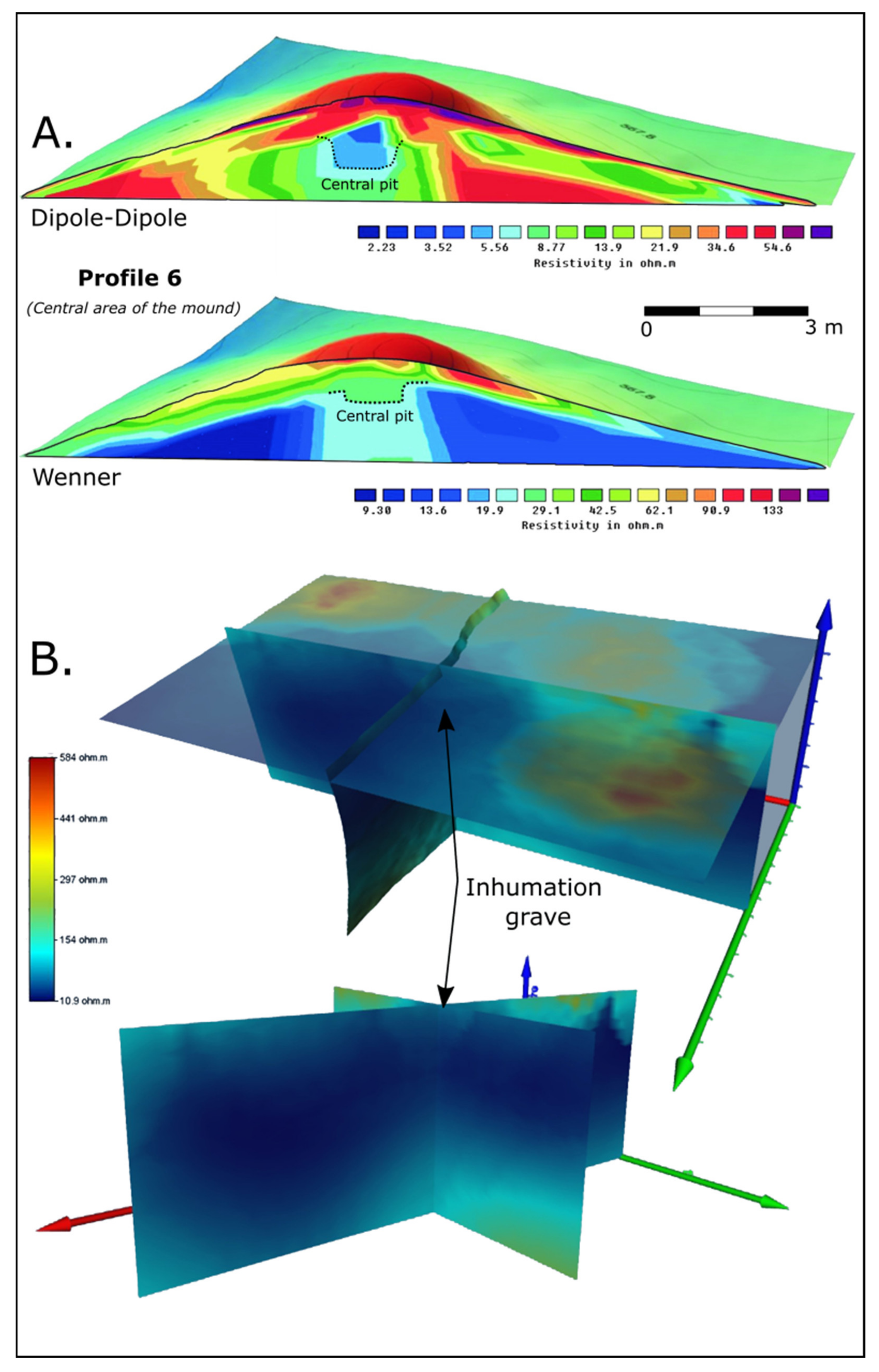
The resistivity values that describe the mound structure are relatively small, with maximum values not exceeding 200 Ωm. In fact, these values describe the electrical properties of the covering mantle. The differences in resistivity revealed the stratigraphy of the mound mantle, which can be described as having at least two distinct levels (Figure 11). In addition to the resistivity values related to the mantle, there are a number of lower values, which describe the intrusions inside the mantle and the geological layer below it. In this way, one can easily distinguish an area with lower values at the center of the mound. This area with values between 5 and 30 Ωm appears on both electrode configurations, Wenner and Dipole–Dipole (Figure 11). We consider that this area represents the central complex, where the deceased was deposited, cremated, or buried. The low values of resistivity can be justified by water infiltration or retention in the soil context of the pit or the cover of the funerary structure. The filling can be represented by another type of clay exhibiting a higher conductivity. The central feature is also visible in the three-dimensional model of resistivity obtained by interpolating the 13 electrical profiles materialized over the mound (Figure 11).
In the case of this central complex structure, there is a good distinction between the elements related to human intervention and those belonging to the geological substrata.
4. Discussion
At M3, systematic excavations were carried out in 2015, 2016, 2017, 2019, and 2020. In 2015–2016 excavation research campaign, trench S1 was dug and then in 2017, 2019, 2020 the north-western corner of the mound was excavated. The 2017 excavation results are illustrated in Diaconescu 2020 [24]. The archaeological report from the 2020 excavation campaign is not published yet. According to Diaconescu and Tincu 2016 [23] and Diaconescu 2020 [24], the excavations revealed the following:
- -
- The stratigraphy of mound M3 is relatively uniform, composed of 4 layers: level 1 corresponding to vegetal layer; level 2 related to the mound’s mantle, consisting of a compact reddish-brown soil; level 3 comprising of a compact brown layer with black-gray intrusions; and level 4 containing a compact clay layer [23].
- -
- The location of the C1 complex and the C3 complex: At a depth of 0.60 m, the central mound complex was identified with a loose filling similar to that of level 3. The extension of the excavation outlined in detail the C3 complex, which turned out to be an inhumation grave. The grave housed a human skeleton sitting on its back, with its legs flexed and its head facing west. In the filling of the grave, a strip of yellow soil (approx. 2 cm) was described in a quadrilateral shape around the skeleton. In fact, this strip of soil explains that the deceased was deposited in a wooden box, which once buried was exerted to pressure due to the filling soil and caused post-mortem skeletal fractures. Subsequently, C3 was identified with M1/2015 magnetic anomaly, and C1 as the grave arrangement shaft within the mound [23].
- -
- The case of the C2, C5, and C6 features: This cluster of features was outlined with the extension and deepening of the excavation to the west. Features C2, C5, and C6 were dug in level 4—the earliest level—and feature C2 had a rectangular shape. It consisted of three rows of beams superimposed alternately in terms of direction, the first row (the lower one) having an N-S direction, the second (the middle one) an E-W direction, and the last one (the upper one) again N-S direction. It has to be mentioned that this complex was heavily set on fire. Ceramic vessels were deposited over the beam structure. Other ceramic vessels were discovered nearby [23]. The best overview for these findings is provided by Diaconescu 2020 [24]. C5 is a shallow pit situated in direct correlation to C2, but slightly below it and contains cremated human bones from two individuals (Diaconescu 2020, 22, n. 37) [24]. C6 is a foundation ditch containing two posts (C6A and C6B) that were used to create an originally horizontal position for the beam structure C2.
The presence of the magnetic anomalies in the center of the mound are due to the archaeological material found within the C1 and C2 features. The difference in the magnetic susceptibility related to the filling of C1 and the heavily burned structure of C2 generated a significant response in the central part of the mound. However, the response of C2 was greatly diminished by the existence of the layer that constitutes the mantle of the mound.
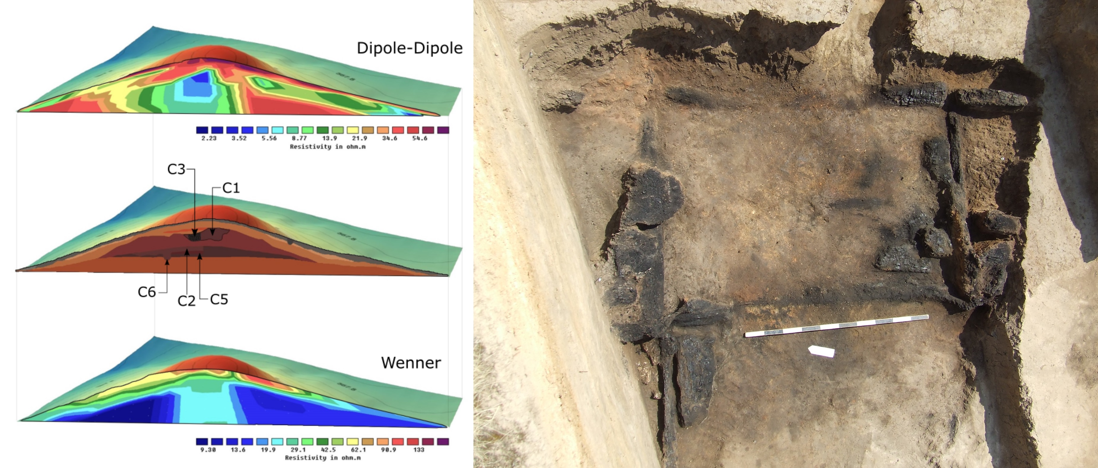
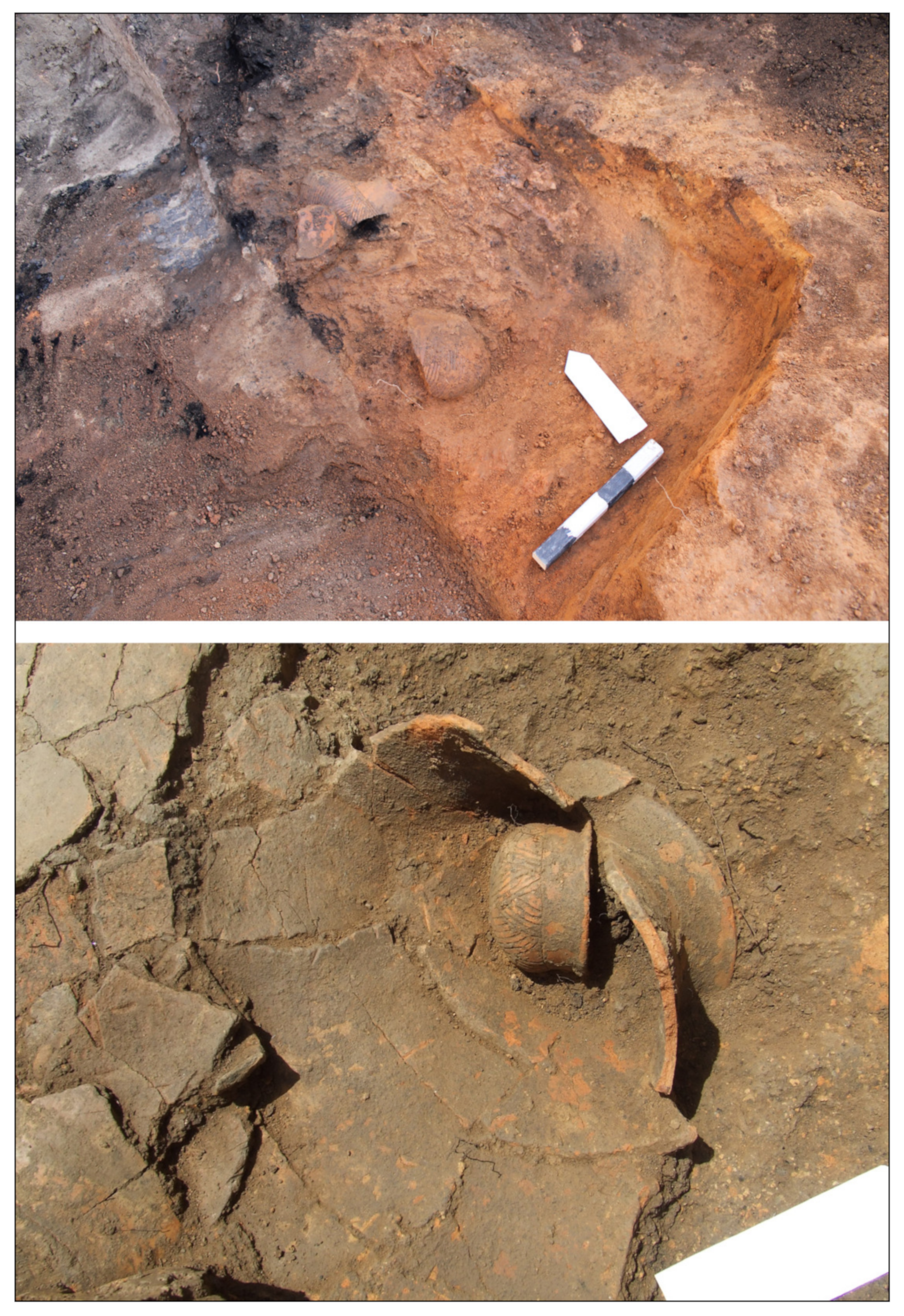
The amplitude of a magnetic anomaly can vary depending on the thickness of the upper layer. In addition to ceramic materials, a significant contribution to the generation of the anomaly was attributed to the vitrified clay that covered the burned beams, as well as the beams themselves (Figure 12 and Figure 13). The structure of the beams (Figure 12c) was documented archaeologically and represents the reason why the mound was built—being, stratigraphically speaking, the earliest archaeological feature inside it [23].
If we compare the current archaeological documentation with the geomagnetic map (Figure 14), we can launch the hypothesis that the magnetic anomalies 2, 3, 4 represent similar structures, namely pits containing a substantial amount of archaeological material. Their location suggests that they do not belong to the same stratigraphic level with anomaly 1. Most likely, these anomalies represent later burial graves within the mound’s mantle.
Unfortunately, the geomagnetic measurements cannot highlight the stratigraphic difference among archaeological features. After all, the most prominent changes of the local magnetic field are represented. Given the stratigraphic overlap, establishing relative relations between archaeological features remained the desideratum of applying complementary geophysical methods.
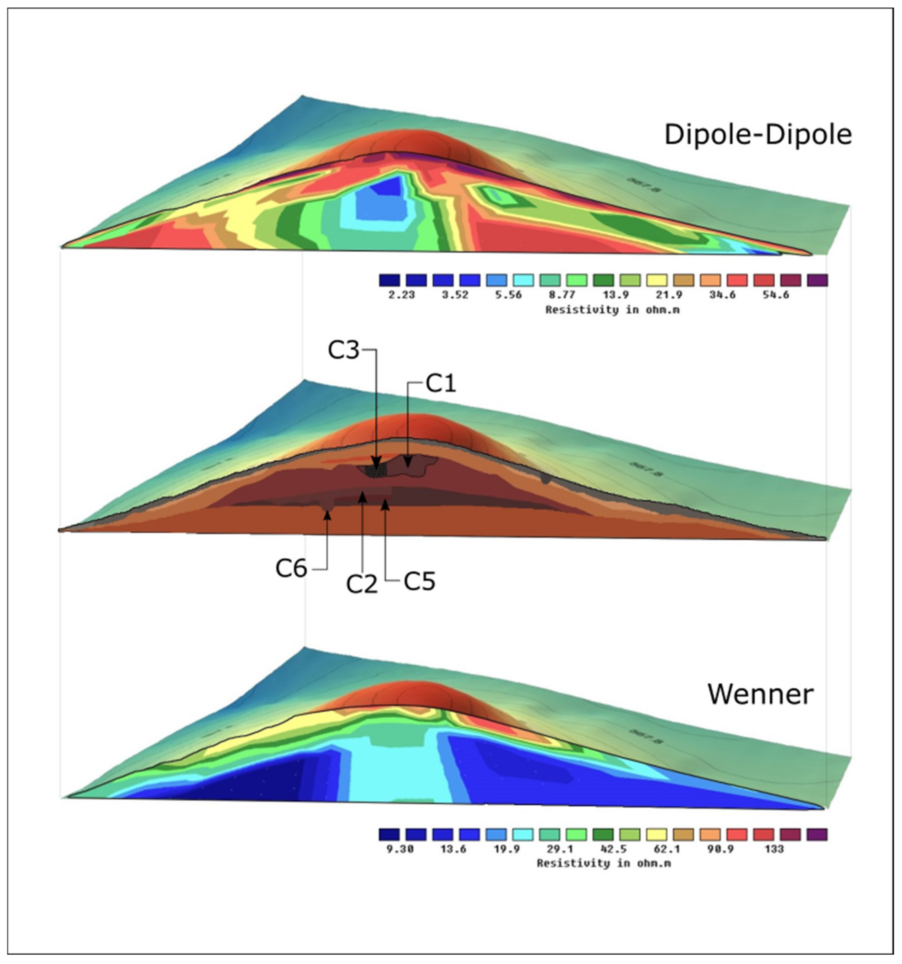
The comparison between the archaeological excavation of the northern section of the mound with the ERT Profile 6 confirmed the existence of C1 and C3 (M1/2015). At the same time, the resistivity results showed similarities with the archaeological results in terms of the mound’s stratigraphy (Figure 15).
The Wenner electrode configuration accurately highlighted the existence of feature C1, while the dipole–dipole array highlighted M1/2015 (C3) and C1. The lower values of resistivity within the archaeological features were caused by the higher moisture in the filling of the pits. This can be grasped on ERT Profile 6 (Figure 15). Finally, the geoelectric measurements highlighted the contact interface between the anthropogenic levels and the nearby geological layers.
5. Conclusions
The geomagnetic measurements allowed us to precisely identify and map the archaeological features (seen as anomaly 1, 2, 3, 4, and 5) inside the M3 mound even if most of the structures are covered by a thick layer of clay (the mantle). The central anomaly defined the central grave, which is the reason for the mound to be constructed. The distribution of anomalies suggest that the mound should have been used as a burial place more than once, as the anomalies are representing pits filled with the soil of different susceptibility compared to the compacted layer of the mantle. These secondary pits (burials) were most probably excavated at a later time after the mound was built.
The ERT survey precisely identified the central feature of the mound, which is visible on both Wenner and Dipole–Dipole electrode configurations, and outlined an inhumation grave-pit which was excavated at a later time after the mound was built.
The archaeological excavations validated the hypothesis raised by the geophysical results and proved that the mound was initially used as a cremation ceremonial locus in which the funerary pyre was built, burned, and covered with a compact layer of clay during the third phase of the Coțofeni culture and that there is a second use of the mound on a later date. The second stage of Dealu Țapului necropolis is directly connected to Yamnaya culture/Yamnaya cultural influences. The Yamnaya people re-used the mound by placing an inhumation grave defined during the archaeological excavation as C3 (M1/2015), which was perfectly visible on ERT (Dipole–Dipole) profile 6.
The interdisciplinary research from Silvașu de Jos—Dealu Țapului offers the possibility to assert that tumuli cemeteries were used for the first time in western Romania by the Coțofeni culture, during a younger chronological phase. It also provides support to identify the missing link, from the territorial perspective, for Yamnaya culture by connecting the discoveries from the Banat region to those from central Transylvania (Cluj area).
Based on the above results we can conclude that geomagnetic and electrical resistivity tomography (ERT) are efficient to identify and map the archaeological features inside the mounds of the necropolis located in Silvașu de Jos—Dealu Țapului, suggesting that this combination of methods can be further applied to the exploration of anther tumular necropolis across Romania.
Author Contributions
Conceptualization, A.H. and D.D.; methodology, A.H.; software, A.H.; validation, D.D.; formal analysis, A.H., A.S., M.P. and A.O.; investigation, A.H., P.U. and D.D.; resources, A.H.; data curation, A.H., A.S. and M.P.; writing—original draft preparation, A.H.; writing—review and editing, D.D., A.S., P.U., M.P. and A.O.; visualization, A.H.; supervision, A.H.; project administration, A.H. and D.D.; funding acquisition, A.H. and A.S. All authors have read and agreed to the published version of the manuscript.
Funding
This research was funded by supported by hardware resources through the Big Data Science grant PN-III-P1-PFE–28 and partially by a grant of Ministry of Research and Innovation, CNCS—UEFISCDI, project number PN-IIIP1–1.1-PD–2019-0939, within PNCDI III.
Institutional Review Board Statement
Not applicable.
Informed Consent Statement
Not applicable.
Data Availability Statement
The data presented in this study are available on request from the corresponding author.
Acknowledgments
We are grateful to Immo Trinks, Martin Roseveare, Ivan Rdev, and Joep Orbons, members of Geophysical Prospection in Archaeology Facebook group, for providing insights regarding our magnetic map.
Conflicts of Interest
The authors declare no conflict of interest.
References
- Nikulka, F. Bronze Age Burial Mounds in Northern and Central Europe: Their Origins and the Development of Diversity in Time and Space. In Burial Mounds Europe and Japan Comparative Contextual Perspectives; Knopf, T., Steinhaus, W., Fukunasa, S., Eds.; Archaeopress: Summertown, UK, 2018; pp. 47–56. [Google Scholar]
- Ballmer, A.T. Burial Mound/Landscape-Relations. Approaches put forward by European Prehistoric Archaeology. In Burial Mounds Europe and Japan Comparative Contextual Perspectives; Archaeopress: Summertown, UK, 2018. [Google Scholar]
- Parzinger, H.; Gass, A.; Fassbinder, J. At the Foot of Royal Kurgans. The latest geoarchaeological and geophysical studies. Sci. First Hand 2016, 43, 74–89. [Google Scholar]
- Guyot, A.; Hubert-Moy, L.; Lorho, T. Detecting Neolithic burial mounds from LiDAR-derived elevation data using a multi-scale approach and machine learning techniques. Remote Sens. 2018, 10, 225. [Google Scholar] [CrossRef] [Green Version]
- Trier, Ø.D.; Larsen, S.Ø.; Solberg, R. Automatic detection of circular structures in high-resolution satellite images of agricultural land. Archaeol. Prospect. 2009, 16, 1–15. [Google Scholar] [CrossRef]
- Orengo, H.A.; Conesa, F.C.; Garcia-Molsosa, A.; Lobo, A.; Green, A.S.; Madella, M.; Petrie, C.A. Automated detection of archaeological mounds using machine-learning classification of multisensor and multitemporal satellite data. Proc. Natl. Acad. Sci. USA 2020, 117, 18240–18250. [Google Scholar] [CrossRef] [PubMed]
- Sărășan, A.; Ardelean, A.-C.; Bălărie, A.; Wehrheim, R.; Tabaldiev, K.; Akmatov, K. Mapping burial mounds based on UAV-derived data in the Suusamyr Plateau, Kyrgyzstan. J. Archaeol. Sci. 2020, 123, 105251. [Google Scholar] [CrossRef]
- Fassbinder, J.W.E.; Gorka, T.; Parzinger, H.; Nagler, A. Magnetic prospection of Scythian Kurgans from Chilik, Southeastern Kazakhstan. ArcheoSci. Rev. D’archéométrie 2009, 59–61. [Google Scholar] [CrossRef] [Green Version]
- Gorka, T.; Fassbinder, J.W.E. Classification and Documentation of Kurgans by magnetometry. In Proceedings of the Archaeological Prospection, Extended Abstracts, 9th International Conference on Archaeological Prospection, Izmir, Turkey, , 19–24 September 2011; pp. 183–186. [Google Scholar]
- Bondar, K.M.; Daragan, M.M.; Prilukov, V.; Polin, S.V.; Tsiupa, I.V.; Didenko, S.V. Magnetometry of the Scythian burial ground Katerinovka in the Lower Dnieper region. Geofiz. Zhurnal 2019, 41, 134–152. [Google Scholar] [CrossRef]
- Papadopoulos, N.G.; Yi, M.-J.; Kim, J.-H.; Tsourlos, P.; Tsokas, G.N. Geophysical investigation of tumuli by means of surface 3D electrical resistivity tomography. J. Appl. Geophys. 2010, 70, 192–205. [Google Scholar] [CrossRef]
- Chen, R.; Tian, G.; Zhao, W.; Wang, Y.; Yang, Q. Electrical resistivity tomography with angular separation for characterization of burial mounds in southern china. Archaeometry 2018, 60, 1122–1134. [Google Scholar] [CrossRef]
- Tsourlos, P.; Papadopoulos, N.; Yi, M.-J.; Kim, J.-H.; Tsokas, G. Comparison of measuring strategies for the 3-D electrical resistivity imaging of tumuli. J. Appl. Geophys. 2014, 101, 77–85. [Google Scholar] [CrossRef]
- Schneidhofer, P.; Nau, E.; Leigh McGraw, J.; Tonning, C.; Draganits, E.; Gustavsen, L.; Trinks, I.; Filzwieser, R.; Aldrian, L.; Gansum, T. Geoarchaeological evaluation of ground penetrating radar and magnetometry surveys at the Iron Age burial mound Rom in Norway. Archaeol. Prospect. 2017, 24, 425–443. [Google Scholar] [CrossRef]
- Schneidhofer, P.; Nau, E.; Hinterleitner, A.; Lugmayr, A.; Bill, J.; Gansum, T.; Paasche, K.; Seren, S.; Neubauer, W.; Draganits, E. Palaeoenvironmental analysis of large-scale, high-resolution GPR and magnetometry data sets: The Viking Age site of Gokstad in Norway. Archaeol. Anthropol. Sci. 2017, 9, 1187–1213. [Google Scholar] [CrossRef]
- St Pierre, E.; Conyers, L.; Sutton, M.; Mitchell, P.; Walker, C.; Nicholls, D. Reimagining life and death: Results and interpretation of geophysical and ethnohistorical investigations of earth mounds, Mapoon, Cape York Peninsula, Queensland, Australia. Archaeol. Ocean. 2019, 54, 90–106. [Google Scholar] [CrossRef]
- Conyers, L.B.; St Pierre, E.J.; Sutton, M.; Walker, C. Integration of GPR and magnetics to study the interior features and history of earth mounds, Mapoon, Queensland, Australia. Archaeol. Prospect. 2019, 26, 3–12. [Google Scholar] [CrossRef]
- Goodman, D.; Hongo, H.; Higashi, N.; Inaoka, H.; Nishimura, Y. GPR surveying over burial mounds: Correcting for topography and the tilt of the GPR antenna. Near Surf. Geophys. 2007, 5, 383–388. [Google Scholar] [CrossRef]
- Badea, L.; Urucu, V.; Gruescu, I. Dealurile Hunedoarei şi Culoarul Streiului. Geogr. României III Carpaţii Româneşti şi Depresiunea Transilv. Bucureşti Ed. Acad. Române 1987, 3, 354–360. [Google Scholar]
- Mureşan, M.; Mureşan, G.; Kräutner, H.G.; Kräutner, F.; Ţicleanu, N.; Stancu, J.; Popescu, A.; Popescu, G. Harta Geologică 1:50 000, Foaia 89 d, Hunedoara; Geological Institute of Bucharest: Bucharest, Romania, 1980. [Google Scholar]
- Luca, S.A.; Diaconescu, D.; Roman, C.; Tincu, S. Cercetările arheologice de la Silvaşu de Jos-Dealul Ţapului. Campaniile anilor 2006–2010. Anu. Muz. Bucov. 2011; 38, 7–54. [Google Scholar]
- Luca, S.A.; Diaconescu, D.; Roman, C.C.; Tincu, S. The Archaeological Research from Silivaşu de Jos-Dealul Ţapului. The Archaeological Campaigns from 2006–2010. 2011. Available online: https://www.academia.edu/2764918/The_Archeological_research_from_Silva%C8%99u_de_Jos_Dealul_%C5%A2apului_The_Archaeological_campaigns_from_2006_2010_in_Seria_Interferen%C5%A3e_etnice_%C5%9Fi_culturale_%C3%AEn_mileniile_I_a_Chr_I_p_Chr_Vol_XX_Ed_C%C4%83lin_Cosma (accessed on 6 January 2021).
- Diaconescu, D.; Tincu, S. Considerații arheologice privind necropola tumulară de la Silvașu de Jos-Dealu Țapului (oraș Hațeg, jud. Hunedoara). An. Banat. 2016, 24, 107–141. [Google Scholar]
- Diaconescu, D. Step by steppe: Yamnaya culture in Transylvania. Praehist. Z. 2020, 95, 17–47. [Google Scholar] [CrossRef]
Figure 1.
Location of Silvașu de Jos—Dealu Țapului (A,B); Google Earth image of the site (C). The archaeological excavation is visible inside the red circle.
Figure 1.
Location of Silvașu de Jos—Dealu Țapului (A,B); Google Earth image of the site (C). The archaeological excavation is visible inside the red circle.

Figure 2.
Distribution of discovered mounds within the area.

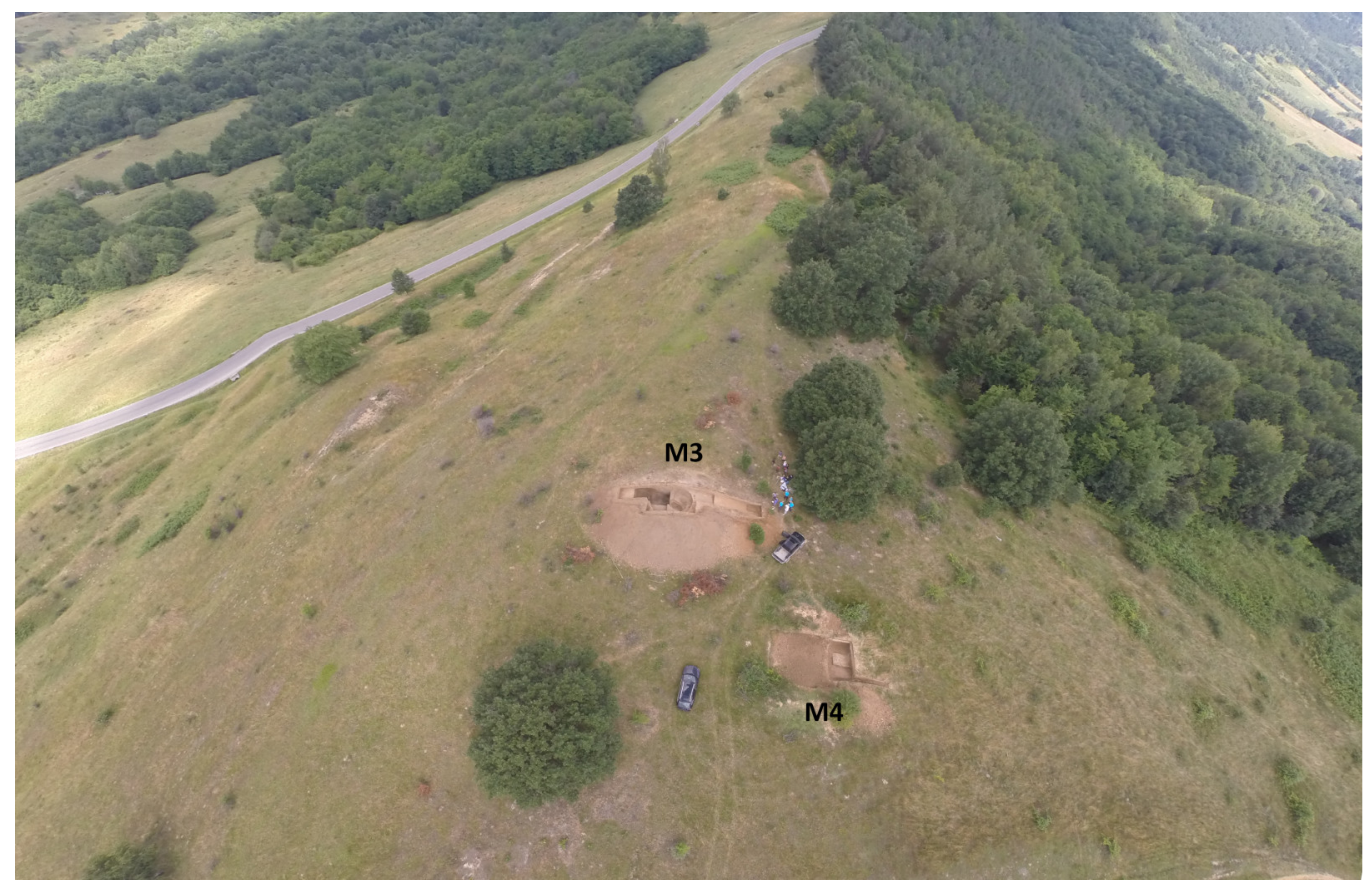
Figure 3.
Drone photography of M3 and M4 excavation (Photo credit: InfoHD).

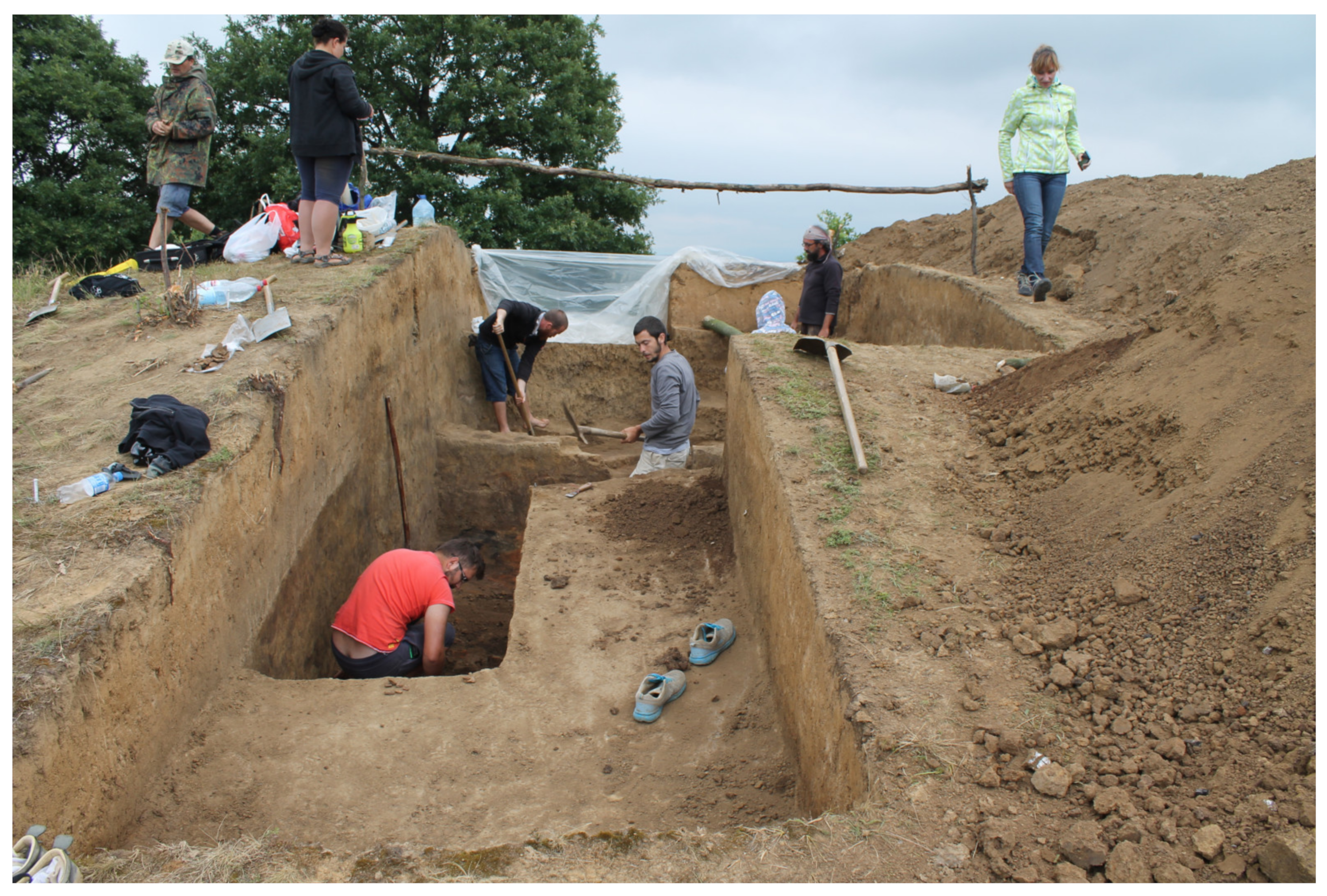
Figure 4.
Excavation progress picture (Dragoș Diaconescu’s photo archive).

Figure 5.
(A) Elevation distribution in the dataset; (B) Measured points in the field; (C) Interpolation.
Figure 5.
(A) Elevation distribution in the dataset; (B) Measured points in the field; (C) Interpolation.

Figure 6.
Areas where the geophysical survey was carried out (black for geomagnetic survey and red for electrical resistivity tomography) overlayed by the later archaeological excavation boundaries (with blue).
Figure 6.
Areas where the geophysical survey was carried out (black for geomagnetic survey and red for electrical resistivity tomography) overlayed by the later archaeological excavation boundaries (with blue).

Figure 7.
The pattern of walking direction during data acquisition with Geometrics G858G (right). Left: the position of the proton magnetometer Geometrics G857.
Figure 7.
The pattern of walking direction during data acquisition with Geometrics G858G (right). Left: the position of the proton magnetometer Geometrics G857.

Figure 8.
Position of each electrical resistivity tomography (ERT) electrode during the field measurements.
Figure 8.
Position of each electrical resistivity tomography (ERT) electrode during the field measurements.

Figure 9.
Basic morphometrical parameters of the mound: elevation model (on the top), elevation map (bottom left), and slope distributions (bottom right).
Figure 9.
Basic morphometrical parameters of the mound: elevation model (on the top), elevation map (bottom left), and slope distributions (bottom right).

Figure 10.
Geomagnetic map (dynamics −3 to +3 nT) of the mound overlayed by the mound contours extracted from the digital elevation model.
Figure 10.
Geomagnetic map (dynamics −3 to +3 nT) of the mound overlayed by the mound contours extracted from the digital elevation model.

Figure 11.
ERT results: (A) Profile 6 (Wenner and Dipole–Dipole) passing the center of the mound and close to the northern side of the archaeological excavation; (B) Cross-sections extracted from the ERT 3D model (a grave pit is faintly visible in the center of the mound, later the excavation confirmed the existence of an inhumation grave—M1/2015—C3).

Figure 12.
(A) The excavation plan presented by Diaconescu 2020 [24]; (B) Drone image taken during the archaeological excavation where the C1, C2, and C3 are visible (Photo: InfoHD); (C) Depiction of feature C2 after the removal of vitrified clay layer—the preserved beams are coming from the funerary pyre which was cover by the layer 3 (Photo: Dragoș Diaconescu).

Figure 13.
Burned layer and archaeological pottery “in situ” (Dragoș Diaconescu’s photo archive).

Figure 14.
The archaeological excavation plan presented in Diaconescu 2020 [24] overlayed on the magnetic map (left). On the right, a detailed view of the excavated archaeological features matching the magnetic anomaly M1, located in the central part of the mound, is provided.
Figure 14.
The archaeological excavation plan presented in Diaconescu 2020 [24] overlayed on the magnetic map (left). On the right, a detailed view of the excavated archaeological features matching the magnetic anomaly M1, located in the central part of the mound, is provided.

Figure 15.
A comparison between ERT Profile 6 and the archaeological excavation northern profile presented in Diaconescu 2020 [24]. Archaeological feature C1 is visible on both configurations (Wenner and Dipole–Dipole), while C3 also called M1/2015 (a grave which was latter dug in the mantle of the mound) is clearly visible on Dipole-Dipole configuration. The main layers of the mound’s stratigraphy are also visible on the ERT profile.

Publisher’s Note: MDPI stays neutral with regard to jurisdictional claims in published maps and institutional affiliations. |
© 2021 by the authors. Licensee MDPI, Basel, Switzerland. This article is an open access article distributed under the terms and conditions of the Creative Commons Attribution (CC BY) license (http://creativecommons.org/licenses/by/4.0/).
Share and Cite
MDPI and ACS Style
Hegyi, A.; Diaconescu, D.; Urdea, P.; Sarris, A.; Pisz, M.; Onaca, A. Using Geophysics to Characterize a Prehistoric Burial Mound in Romania. Remote Sens. 2021, 13, 842. https://doi.org/10.3390/rs13050842
AMA Style
Hegyi A, Diaconescu D, Urdea P, Sarris A, Pisz M, Onaca A. Using Geophysics to Characterize a Prehistoric Burial Mound in Romania. Remote Sensing. 2021; 13(5):842. https://doi.org/10.3390/rs13050842
Chicago/Turabian StyleHegyi, Alexandru, Dragoș Diaconescu, Petru Urdea, Apostolos Sarris, Michał Pisz, and Alexandru Onaca. 2021. "Using Geophysics to Characterize a Prehistoric Burial Mound in Romania" Remote Sensing 13, no. 5: 842. https://doi.org/10.3390/rs13050842
Note that from the first issue of 2016, this journal uses article numbers instead of page numbers. See further details here.