Time Evolution of Storms Producing Terrestrial Gamma-Ray Flashes Using ERA5 Reanalysis Data, GPS, Lightning and Geostationary Satellite Observations

Abstract

In this article, we report the first investigation over time of the atmospheric conditions around terrestrial gamma-ray flash (TGF) occurrences, using GPS sensors in combination with geostationary satellite observations and ERA5 reanalysis data. The goal is to understand which characteristics are favorable to the development of these events and to investigate if any precursor signals can be expected. A total of 9 TGFs, occurring at a distance lower than 45 km from a GPS sensor, were analyzed and two of them are shown here as an example analysis. Moreover, the lightning activity, collected by the World Wide Lightning Location Network (WWLLN), was used in order to identify any links and correlations with TGF occurrence and precipitable water vapor (PWV) trends. The combined use of GPS and the stroke rate trends identified, for all cases, a recurring pattern in which an increase in PWV is observed on a timescale of about two hours before the TGF occurrence that can be placed within the lightning peak. The temporal relation between the PWV trend and TGF occurrence is strictly related to the position of GPS sensors in relation to TGF coordinates. The life cycle of these storms observed by geostationary sensors described TGF-producing clouds as intense with a wide range of extensions and, in all cases, the TGF is located at the edge of the convective cell. Furthermore, the satellite data provide an added value in associating the GPS water vapor trend to the convective cell generating the TGF. The investigation with ERA5 reanalysis data showed that TGFs mainly occur in convective environments with unexceptional values with respect to the monthly average value of parameters measured at the same location. Moreover, the analysis showed the strong potential of the use of GPS data for the troposphere characterization in areas with complex territorial morphologies. This study provides indications on the dynamics of con-vective systems linked to TGFs and will certainly help refine our understanding of their production, as well as highlighting a potential approach through the use of GPS data to explore the lightning activity trend and TGF occurrences.

1. Introduction

In 1994, a surprising observation by the National Aeronautics and Space Administration (NASA) Compton Gamma-Ray Observatory (CGRO) detected unexpected gamma-ray emissions coming from the Earth [1]. These so-called terrestrial gamma-ray flashes (TGFs), produced inside storms in association with lightning with typical durations of less than 1 millisecond and energies up to few tens of MeV [2], are the manifestation of the most energetic natural particle accelerators on Earth, strong enough to be observed by highly sensitive instruments orbiting in space. In particular, the Reuven Ramaty High Energy Solar Spectroscopic Imager (RHESSI) has observed TGFs for almost 17 years, between 2001 and 2018 [3], and nowadays, TGFs are continuously observed by Fermi [4], the Astro-rivelatore Gamma ad Immagini Leggero (AGILE) [5] and the Atmosphere-Space Interactions Monitor (ASIM) [6] missions.

For decades, this became a topic of frontier research between two disciplines: high-energy physics and atmospheric physics. The first investigated the mechanisms of production, discovering that TGFs are produced by a large number of charged particles accelerated within thunderstorm and lightning intense electric fields, undergoing avalanche multiplication and subsequently emitting gamma-ray photons via bremsstrahlung [2]. On the other hand, to understand under which boundary conditions this phenomenon can trigger and propagate in air, or how rare it is, we need to involve atmospheric sciences. Understanding the rarity, formation and evolution of these atmospheric phenomena is important in assessing the risks to which we are subjected: the authors of [7] pointed out that in the TGF production area, the radiation levels are high enough to compromise health as well as electronics onboard aircraft.

From the meteorological point of view, TGFs are produced by storms of all shapes and sizes, but it is still unknown why some thunderstorms produce gamma-ray bursts and others do not. Several studies in the last decade sought, as the objective, to find correlations between TGFs and meteo/lightning characteristics of the associated events. The authors of [8] conducted an extensive study of storms associated with individual RHESSI TGFs and compared the TGF distribution to maps of water vapor and ice content. The results showed that the ice content had a poor correlation with the TGFs but that the liquid water content in the 10–14 km altitude range, indicating deep convection, provided a much better match. The authors found that storm systems of all sizes could produce TGFs, showing a range in areal extent of several orders of magnitude. The authors of [9], using radio atmospherics data from the World Wide Lightning Location Network (WWLLN), conducted the first analysis on the electrical evolution of a storm related to a TGF event, finding a clear decline in the flash rate surrounding the TGF occurrence, suggesting that TGFs occur preferentially during the declining phase of flash production. In contrast, [10,11] showed that TGFs tend to take place during the peak of the cooling phase, when the lightning flash rate is at its maximum.

Detailed meteorological observations over 24 TGFs detected by Fermi were provided by [12]. They compared the convective available potential energy (CAPE) value at the TGF occurrence with the minimum, mean and maximum CAPE value registered on all days of the month at the same location and time of day. The convective available potential energy (CAPE) values were calculated by the NCEP North American Regional Reanalysis (NARR) dataset [13], with spatial and temporal resolutions of ~2 km and 3 h, respectively. This study showed that the 24 TGFs originated from storms of a wide range of convective strengths, without any clear common characteristics. These results were confirmed also by the recent study of [11] that linked TGF production to cloud instantaneous and dynamical features as extracted by visible–infrared geostationary satellite sensors.

On the other hand, the authors of [14], taking advantage of a satellite-borne radar onboard the Global Precipitation Measurement (GPM) mission [15], performed an analysis of TGF events from a new perspective. A total of 9 TGF-producing storms were analyzed both with active and passive instruments, finding common features: both views agree in describing TGF-producing clouds as intense thunderstorms with significant vertical development and ice content and 100% of the cases presented a cumulonimbus tower. Moreover, all TGF-related lightning is classified as high-amplitude intracloud (IC) flashes. Furthermore, as TGFs are related to lightning, it is essential to try to correlate the issue of the lightning initiation within clouds and its microphysical content processes. In understanding the lightning initiation, tropospheric water vapor content and its dynamics over time could play a key role. In particular, the correlations between lightning activity and tropospheric water vapor (WV) content were analyzed by [16], showing that the maximum/minimum extremely low frequency (ELF: 1 Hz < f < 100 Hz) signal often precedes the maximum/minimum of water vapor measurements on a daily basis.

However, monitoring WV dynamics over time is very difficult. The possibility to measure precipitable WV using the Global Positioning System (GPS) was first explored by [17,18]. The authors of [19], combining integrated precipitable water vapor data from a GPS receiver with other meteorological data, found an important trend anomaly up to about 12.5 h before the first lightning strike, able to predict lightning. In order to identify recurrent patterns useful for improving nowcasting applications, [20] combined estimates of the WV content from the GPS signal with visible–infrared measurements from the Meteosat Second Generation (MSG) and with the lightning activity collected by the ground-based lightning detection network (LINET). They found specific trends appearing before the peak of lightning activity on a timescale from 2 to 3 h. Under this hypothesis, in this work, the search for the boundary conditions around the lightning that triggers a TGF was conducted by analyzing the storm features distribution in time using in situ and satellite data. The scope is to understand which conditions are favorable to the development of TGF events and to investigate if any precursor signals can be expected. To do that, TGFs from the AGILE satellite [21,22,23] were considered. The first meteorological conditions in correspondence with TGF occurrences were studied by ERA5 reanalysis and compared with reference values, in order to evaluate the meteorological conditions leading to storms emitting TGFs. Second, the Global Positioning System precipitable water vapor (GPS-PWV) was considered as a good indicator of moisture content and matched with the strokes registered by WWLLN as well as information obtained from geostationary satellites, allowing the time monitoring of the meteorological conditions preceding the TGF occurrence.

The paper is organized as follows: In Section 2, data and instrumentations are described. In Section 3, the results are shown. The last section reports the discussion and conclusions. The acronyms more frequently used in this paper are reported in the following Abbreviations.

2. Instruments and Data

2.1. AGILE MCAL

AGILE is a satellite owned and operated by the Italian Space Agency and dedicated to gamma-ray astrophysics. It was launched on 23 April 2007 into a low Earth orbit (~550 km altitude) with an inclination of 2.5° [24]. The purpose of the mission is to provide a tool with imaging capabilities for gamma-rays with a large field of view, in order to provide better studies on galactic and extragalactic sources. Among the three instruments onboard, the Mini-Calorimeter (MCAL) is the one specific for the detection of gamma-ray transients, covering an energy range from 300 keV to 100 MeV with an absolute time accuracy of ~2 µs [25]. Specifically, when a significant number of counts is detected in a specific time window, the MCAL is triggered and data are downloaded to telemetry. Furthermore, the quasi-equatorial orbit is optimal to observe equatorial regions, where most TGF events take place. In addition to transient sources of cosmic origin, mostly gamma-ray bursts (GRB), the MCAL also acts as an optimal detector for TGFs.

Additional information on MCAL performances is included in [23,25,26]. Additional information on the association between TGF data and lightning data is included in [22]. We analyzed a total of 648 TGFs with an associated lightning sferic from March 2015 to February 2020 detected from the AGILE MCAL instrument, representing an extension of the 3rd AGILE catalog (282 TGFs in the period 2015–2018 [23] (see Figure 1 and Figure 2). In particular, the TGF sample was identified by the association criteria with radio sferics, detected by the WWLLN network [27], which are described in [22].

The global distribution of TGFs shows preferential coastal areas. The empty area covering the east side of South America represents the South Atlantic Anomaly (SAA), where detection is not active. It is important to underline that the peak over Africa, where the electrical activity manifests its distribution peaks on Earth, results as underestimated due to the lower amount of coverage by WWLLN sensors that make the recording of lightning activity difficult. The local time distribution shows a higher rate of events occurring in the early morning as well as in the late afternoon according to [23]. The duration of TGFs, expressed as the t₅₀ parameter, shows a peak at 20–40 µs, consistent with the observations by [28] regarding TGFs with a lightning sferics simultaneous association, confirming the higher WWLLN matches chance with brief TGF durations [22,28]. Concerning the spatial accuracy on WWLLN data, we here assumed an uncertainty of 15 km [27].

2.2. ERA5 Reanalyses

ERA5 reanalysis is the fifth generation of ECMWF (European Centre for Medium-Range Weather Forecasts) atmospheric reanalyses and covers the period from 1950 until five days before the real time. Reanalysis combines, optimally, model data and observations to provide a complete and consistent representation of the atmosphere. This principle is called data assimilation. Reanalysis does not have the constraint of issuing timely forecasts, so there is more time to collect observations compared to the operational analyses. In addition, when going back in time, analyses allow for the ingestion of improved versions of the original observations, providing a benefit to the quality of the reanalysis product. The assimilation system is able to estimate biases between observations and give more weight to good-quality data compared to poor data. The laws of physics allow for estimates at locations where data coverage is low, propagating, in space and time, the impact of observations. ERA5 provides hourly estimates of a large number of atmospheric, land and oceanic climate variables. The data cover the Earth on an 80 km grid and resolve the atmosphere using 137 levels from the surface up to a height of 8.0 km. Data are available for surface and upper model levels and can be interpolated on pressure, isentropic and constant potential vorticity levels. In this paper, the meteorological parameters considered relevant for convection are the convective available potential energy (CAPE; i.e., the amount of potential energy which an air parcel has available for convection), the convection inhibition energy (CIN; i.e., the amount of energy required to lift an air parcel from the surface to its level of free convection), the total column water vapor (TCWV) and the 2 m dew point temperature (T2D; i.e., the temperature at which air at 2 m must be cooled at constant pressure to become saturated with respect to a plane surface of pure water).

2.3. GPS

The acronym GNSS (global navigation satellite system) defines all the constellations of artificial terrestrial satellites for positioning and navigation. In this regard, only the GPS constellation was employed in this specific study. Today, this system is used in many fields, ranging from navigation [29,30] to monitoring applications [31,32,33] and meteorology [20,34,35,36]. For what concerns this latter field, it is useful to remember that in the Earth’s atmosphere, the signal propagation speed changes due to the physical state of the medium which is crossed. Therefore, analysis of the tropospheric delay, basically caused by the presence of gas and water vapor, becomes particularly interesting. Dry air and water vapor molecules in the troposphere affect GNSS signals by lowering their propagation velocities with respect to a vacuum [17,37]. This tropospheric delay can be modeled during GNSS data processing or used as a source of information; in the second case, the parameter known as the zenith total delay (ZTD) is estimated. The ZTD is the delay related to the zenith direction, obtained after introducing a mapping function, which depends on physical parameters, able to project into the zenith direction the signal delay along each single signal path.

In order to better understand if the distribution of single signal paths, called the slant total delay (STD), is well representative of the area of interest, the configuration of pierce points (PPs) referred to the involved GPS receivers is given. The pierce points (PPs) are the intersections between GPS lines of sight and an ideal shell located at a fixed altitude; in this specific case, the shell height was set as the clouds’ altitude. Contributions of dry air, the zenith hydrostatic delay (ZHD), water vapor and the zenith wet delay (ZWD) to the zenith total delay can be separated and estimated [38], with the following relation being valid:

ZTD = ZHD + ZWD

(1)

where ZHD, caused by dry gases present at the troposphere, is easy to model, whereas ZWD, caused by water vapor and condensed water in the form of clouds, is highly variable. It is possible to take into account the effects of differences in altitude between meteorological sensors and GPS receivers [39,40,41] starting from meteorological data of pressure and temperature with appropriate adjustments linked to the use of the relationships derived from the barometric formula [40] and the height correction proposed in [41]. Hence, it is possible to retrieve these by applying gridded Vienna mapping functions [17,37], ZHD estimates and, consequently, ZWD and precipitable water vapor (PWV) values, by performing the appropriate conversion. In this study, meteorological data of pressure and temperature were retrieved from the empirical GPT (Global Pressure and Temperature) model [42], and the PWV data retrieved from GPS measurements were compared to corresponding products provided by ERA5 [43].

Only geodetic receivers were employed; therefore, starting from the dual-frequency observational files (RINEX Version) collected by the devices at a 30-second rate, the pierce points position technique [44], undifferenced phase observation processing, was applied using an ionosphere-free combination in order to estimate ZTD values for each epoch, by daily processing sessions. The involved ancillary products (ephemeris and clocks) were the precise products provided by the International GNSS Service (IGS). Processing was handled by the beta release of goGPS software, version 1.0, written on the basis of older releases [45] by using a new batch least-squares engine. This section may be divided by subheadings. It should provide a concise and precise description of the experimental results and their interpretation, as well as the experimental conclusions that can be drawn.

2.4. GOES

The Geostationary Operational Environmental Satellite (GOES) program started in 1975 when the first satellite was launched under the coordination of the National Aeronautics and Space Administration (NASA) and the National Oceanic and Atmospheric Administration (NOAA). Currently, four GOES series satellites are operating: GOES-13 and GOES-14 and two GOES-R series satellites (GOES-16 and GOES-17). In this work, the GOES-16 data were used. The GOES-16 is located at 75°W, 0° N and provides data at a 10-minute time resolution. The sub-satellite point has a spatial resolution around 1 km, which becomes coarser moving away from it. The GOES-16 was the first satellite of the GOES-R series to mount the Advanced Baseline Imager (ABI) [46,47]. The ABI has 16 spectral bands ranging from visible (VIS) to infrared (IR) electromagnetic spectra in order to characterize the properties of both clouds and atmospheric gases. In this work, we limited use to only one out of the sixteen ABI channels, namely, channel 13. Channel 13, being a "window" channel centered at 10.33 µm, allows retrieving the cloud top temperature by measuring the brightness temperature (TB).

2.5. Himawari

The Himawari program, operated by the Japan Meteorological Agency (JMA), started in 1977. Since the launch of the first satellite, there have been three generations, including GMS, MTSAT and Himawari 8/9 [48]. Currently, Himawari 8/9 satellites are available for operational use. In this work, the Himawari 8 data were used. The satellite entered operational service on 7 July 2015 at 140.7° E, 0° N carrying on the Advanced Himawari Imager (AHI) a visible–infrared radiometer that possesses comparable capabilities to the GOES-R in terms of spatial, spectral and temporal resolutions [49]. The instrument has 16 observational bands, spanning from the visible to thermal infrared bands, useful for retrieving cloud properties. In this work, we used the same GOES-R channel, namely, the channel centered at 10.4 µm, for the retrieval of the cloud top temperature [49].

3. Results

In order to characterize tropospheric conditions at the occurrence of TGFs, the total AGILE database of 648 geo-located events was analyzed in two ways. For each of the available events, the ERA5 reanalysis data were exploited in order to derive statistical properties of the considered meteorological parameters. On the other hand, GPS, lightning and geostationary data were matched for a selected number of case studies. The main selection criteria beyond their identification were to consider a maximum spatial separation between GPS receivers’ location and TGF occurrences. A reasonable space range must take into account the observation geometry of the GPS receiver and the need to observe the cloud as close as possible to the TGF occurrence. Under these conditions, a 45 km space window was selected as a trade-off between requirements, obtaining a total of nine case studies, two of which are shown below.

3.1. ERA5

In this section, we use ERA5 reanalyses [50] to evaluate the meteorological parameters when TGFs are observed and to compare these values with their reference. To compute the values of the meteorological parameters in correspondence with the TGF observations, we interpolated the ERA5 field to the position and time of the TGF occurrence. The spatial interpolation is bilinear, starting from ERA5 fields at a 0.25° horizontal resolution, while the temporal interpolation is linear, from hourly reanalyses.

Reference values for each parameter are computed considering for each TGF all the hourly values of the meteorological parameter for the month and for the position where the TGF is observed. Then, all the data corresponding to the TGF and reference are gathered together and represented by boxplots.

The average value of CAPE when TGFs are recorded is larger than the corresponding reference values for almost all months considered (Figure 3a). This holds for the 25th and 75th percentiles too. This result shows, as expected, that TGFs occur in convective environments. However, the values of CAPE associated with TGFs are largely variable, as shown in Figure 3a, and are not exceptional compared to the reference values of the parameter for the locations and months where/when TGFs are observed. Indeed, the reference maximum and minimum values always include the corresponding values when TGFs are observed. CIN (Figure 3b) is larger when TGFs are observed compared to the reference values, even if the maximum and minimum values of the reference include the maximum and minimum values obtained when TGFs are observed. Convection is associated with a small but positive value of CIN because this avoids a too fast consumption of the available potential energy that would result in shallow or no convection.

TCWV (Figure 3c) is larger when TGFs are recorded compared to the reference values. This occurs when convection is developing, as also shown by the GPS-ZTD analysis discussed in Section 4, but the values of TCWV associated with TGFs are included in the intervals of the reference values, so they are not extreme values. Similar considerations apply for the dew point temperature at the surface. The higher values for TGF events show a larger amount of water vapor at the surface compared to the reference values. This is well explained by the convective environment in which TGFs occur, which has higher than normal humidity at the surface. Overall, the analysis of ERA5 data shows that, while TGFs occur in convective environments, the values of meteorological parameters describing the convective environment are not exceptional. This result was attained also by dividing the whole dataset into two geographic regions: −180 W/50 E (America–Africa) and 50 E/180 E (India–SE Asia–Oceania). However, we prefer to show the results for the whole globe because the analysis is based on a larger number of TGF data.

3.2. Case Studies

The aforementioned case studies are pinpointed by orange diamonds (representing the TGFs) and black dots (representing the GPS receivers) in Figure 4 and Figure 5 (since some TGFs occurred very close to each other, even if on different dates, they overlap in the figures but are clearly reported in

Table 1. Case studies—2015 and 2018. The selection criteria were set according to a 45 km distance between the GPS receiver’s location and the TGF occurrence.

TGF Date-Time	TGF Coordinates	GPS Marker	GPS Coordinates	Distance [km]	r GPS-ERA5
2015.04.13 12:06:36.42	φ = 0.010 λ = 99.540	ABGS	φ = 0.221 λ = 99.388 H = 251.0	28.93	0.46
2015.05.23 21:12:11.55	φ = 0.160	ABGS	φ = 0.221	42.61	−0.05
	λ = 99.430		λ = 99.388 H = 251.0
2015.06.06 13:12:23.09	φ = 5.310	MLKN	φ = 5.353	42.72	0.89
	λ = 102.660		λ = 102.277
			H = 26.9
2018.02.18 21:26:5.48	φ = 1.500 λ = 98.770	BTET	φ = 1.282 λ = 98.644 H = 38.0 φ = 1.202 λ = 98.940 H = 13.1 φ = 1.326 λ = 99.089 H = 45.5	28.04	0.72 −0.81 0.02
		SOBY		38.19
		MSAI		40.42
2018.05.04 06:33:43.59	φ = 1.515 λ = 78.966	SNLR	φ = 1.293 λ = 78.847 H = 6.2 φ = 1.822	28.00	0.91
		TUMA		43.06	0.87
			λ = 78.730 H = 13.2

and

Table 2. Case studies—2019. The selection criteria were set according to a 45 km distance between the GPS receiver’s location and the TGF occurrence.

TGF Date-Time	TGF Coordinates	GPS Marker	GPS Coordinates	Distance [km]	r GPS-ERA5
2019.03.1 610:35:38.43	φ = −2.440 λ = 101.410	LNNG	φ = −2.285 λ = 101.156 H = 42.6 φ = −2.543 λ = 101.091 H = 6.3	33.00	0.87
		MKMK		37.19	0.85
2019.09.05 08:14:32.09	φ = 8.850	ACP6	φ = 9.238	43.20	0.42
	λ = −79.410		λ = −79.409 H = 930.6
2019.11.15 06:40:47.36	φ = −1.750 λ = −78.240	MZEC	φ = −1.493 λ = −78.483	39.31	−0.51
		BIEC	H = 2911.8 φ = −1.447 λ = −78.501 H = 2354.7	44.51	−0.59
2019.11.15 06:41:58.16	φ = −1.680 λ = −78.380	MZEC	φ = −1.493 λ = −78.483 H = 2911.8 φ = −1.447 λ = −78.501 H = 2354.7 φ = −1.651 λ = −78.651 H = 2789.9 φ = −1.364 λ = −78.412 H = 2560.3	23.72	−0.51
		BIEC		29.24	−0.59 −0.78 −0.23
		RIOP		30.31
		VZCY		35.34

). Two out of the nine case studies (green boxes in Figure 4 and Figure 5) are discussed in more depth in Section 3.2.1 and Section 3.2.2, respectively. In particular, the daily trend of PWV values estimated by all the available GPS receivers (within 45 km from the TGF location) and by the ERA5 reanalysis was compared.

As mentioned before, with the aim to characterize tropospheric conditions at TGF occurrence as well as the reliability limits of the PWV derivation techniques (GPS versus ERA5-based techniques), the GPS-PWV was matched with the strokes registered by WWLLN within a 1° × 1° area centered at the TGF location. In addition, the information obtained from geostationary satellites (i.e., GOES or Himawari depending on the location of the considered event) allows the time monitoring of the meteorological conditions preceding the TGF occurrence. It has to be taken into account that each case study was characterized by a distinctive geographical morphology with respect to the others. Each case study is identified through temporal (Date-Time in the first column) and spatial (φ (lat) and λ (lon) as well as altitude H in the fourth column) coordinates (Table 1 and Table 2). Referring to each TGF occurrence, nearby GPS receivers were selected and included in Table 1 and Table 2 by their marker names (third column) and their coordinates (fourth column). Two additional parameters, the distance between the TGF and GPS position and the correlation coefficient, computed on a daily scale, between PWV-GPS and PWV-ERA5, are placed in the last two columns. This last parameter (r) was used in order to compare the operating conditions of the two techniques. As can be seen from the r-values, the correlation is closely linked both to the distance between the TGF occurrence and the GPS receiver and to the morphology of the territory where the phenomenon is located. In fact, the correlation tends to degrade as the orography becomes more complex (high altitudes) and as the distance between the TGF and GPS device increases. This implies a good reliability of ERA5 in cases where the orography is simple (low altitude), although it remains a technique whose values are more smoothed, mainly because of the spatial resolution (wide grid mesh), which inhibits its ability to identify small-scale variability, which is well captured by GPS. In the tables, the case studies described below are marked in bold.

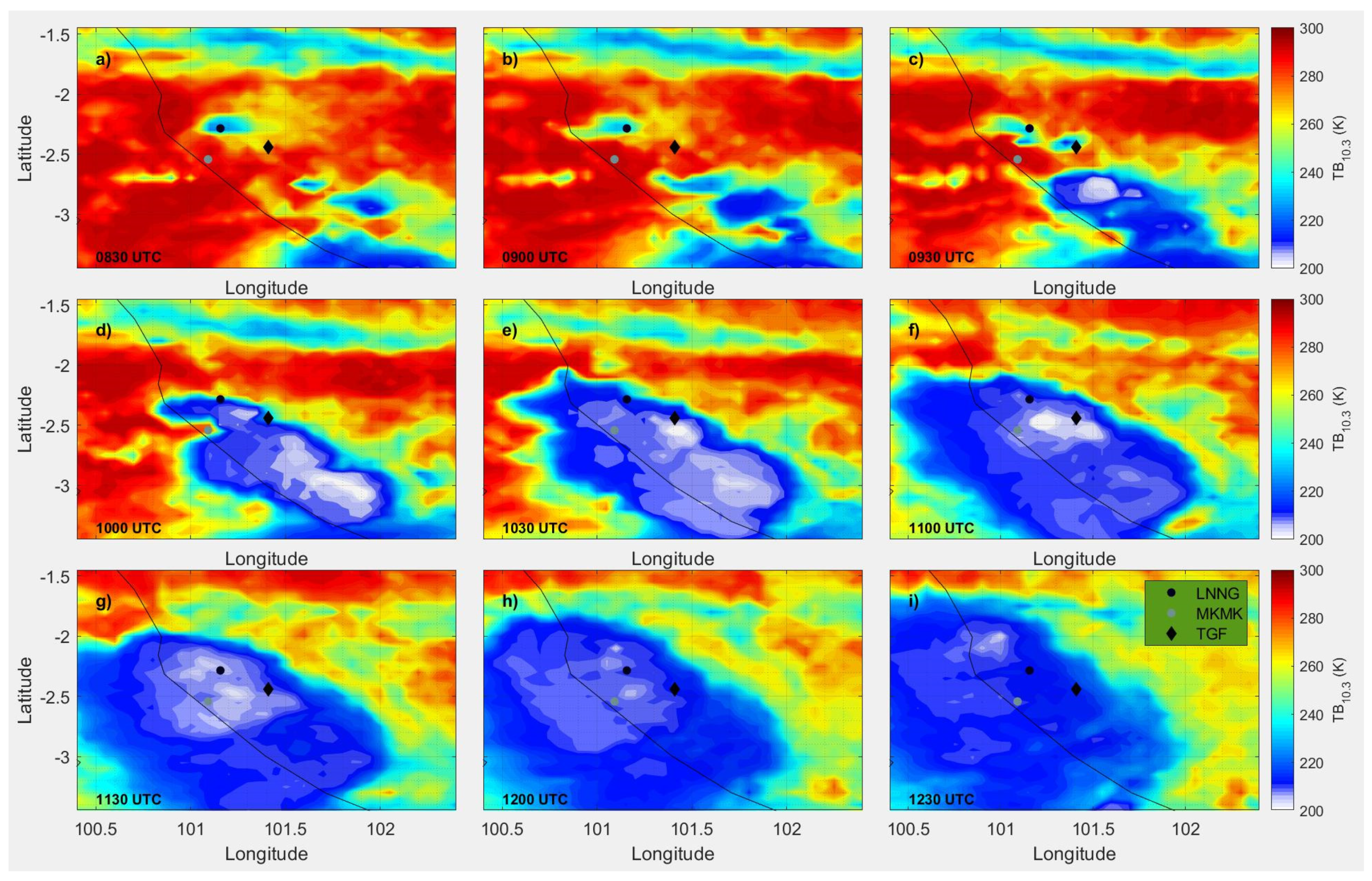
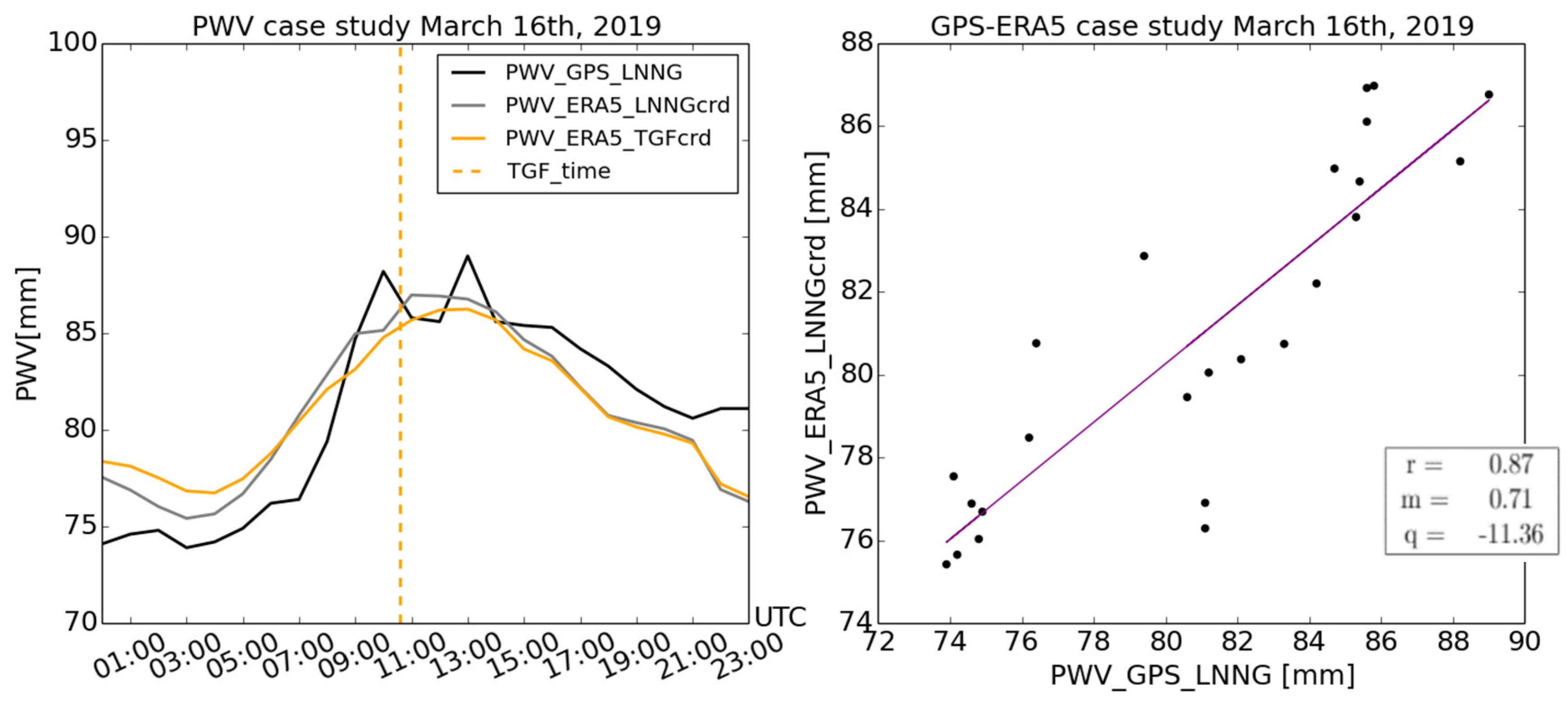
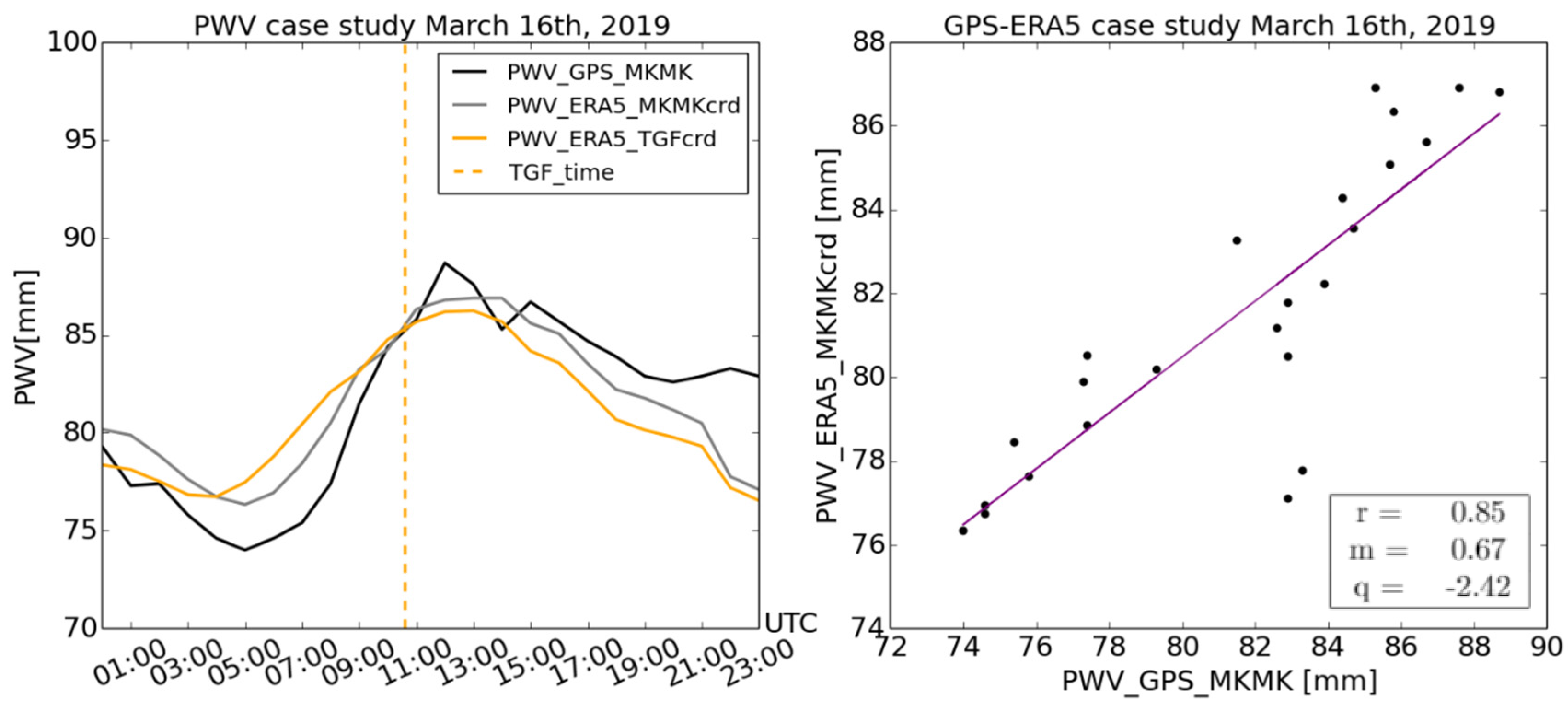
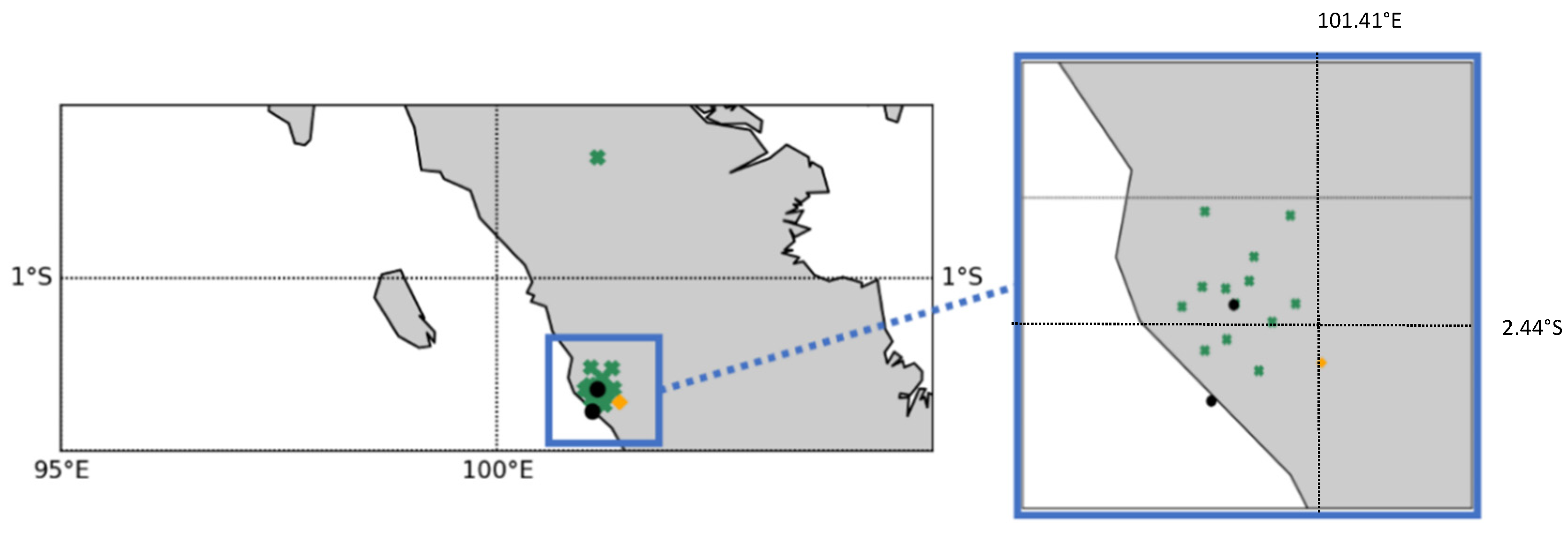
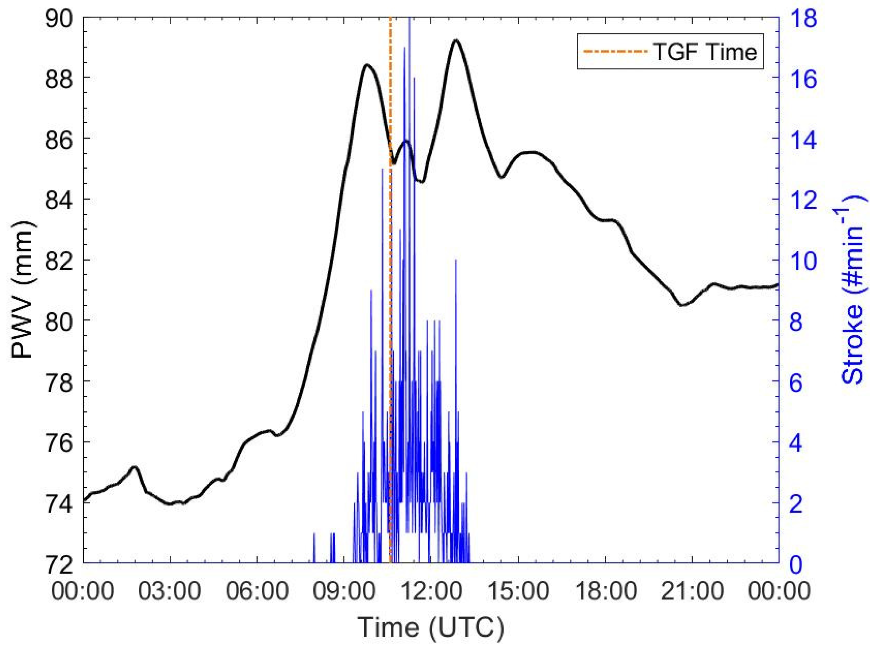
3.2.1. Sumatra—16 March 2019

This first case study concerns an event that occurred near the coast of Sumatra on 16 March 2019. The TGF occurred at 10:35:38 UTC at the following latitude and longitude: φ = −2.44, λ = 101.41. Two GPS receivers, LNNG and MKMK, were placed at 33 and 37 km distances from the TGF location and at an altitude of 42 and 6 m above sea level (a.s.l.), respectively. The growth of the convective cell that will generate the TGF was observed over time (Figure 6).

Satellite images are very useful in order to understand if the PWV variation measured by the GPS receivers is due exclusively to the precipitating system linked to the TGF. The sequence, starting 2 hours before the TGF occurrence (Figure 6a), evidences the growth of the convective cell that will generate the TGF. The TBs reported in Figure 6e (i.e., the Himawari-8 image closest to the TGF time) highlight very deep convection with values up to 205 K. The convective cell reaches its maximum vertical extension in the following 30 min with respect to the TGF (Figure 6e) and then moves to its expiration. Furthermore, the TGF is located at the edge of the convective cell. This feature is common to almost the totality of the cases analyzed. Figure 7 and Figure 8 show a direct comparison, after the bias removal, between PWV-GPS data and PWV-ERA5 data. In particular, panel (a) of each of the two figures reports the daily trend of GPS-PWV (black solid line) and ERA5-PWV at both GPS and TGF coordinates (gray and orange solid lines, respectively). The time of the TGF occurrence is marked by the orange dashed vertical line. On the other hand, panel (b) shows the scatterplot between GPS-PWV and ERA5-PWV.

The scatterplots show a high correlation between GPS-PWV and ERA5-PWV for both GPS receivers with r_LNNG=0.87 and r_MKMK=0.85, respectively (see Table 2); this means that in this specific and similar circumstance (not particularly complex territorial morphology), it is possible to use the ERA5-PWV dataset in order to evaluate the PWV behavior at TGF coordinates. Comparing the GPS-PWV trend with the ERA5 trend at TGF coordinates, a slight offset between curves can be identified (Figure 7), which is related to the structure of the convective clouds and to the position of GPS sensors in relation to TGF coordinates. In Figure 9, the distribution of pierce points (PPs), that is, the intersections between GPS lines of sight and an ideal shell located at the clouds’ altitude, referred to the LNNG GPS receiver is given. The aim is to analyze the configuration of PPs with respect to the GPS receiver. The analysis shows that the PPs are well distributed around the GPS receiver and close to the event; therefore, the GPS-PWV trend (Figure 7) can be considered well representative of the water vapor content within the area of the TGF occurrence.

Finally, the GPS-PWV trend is compared with the stroke rate trend registered by the WWLLN measurements within a 1° × 1° area centered at the TGF location (Figure 10). The TGF occurred after the marked increase in PWV reached a local maximum at about 09:30 UTC. On the other hand, the TGF preceded the maximum stroke rate that occurred at about 11:00 UTC, with values reaching 16 strokes/min.

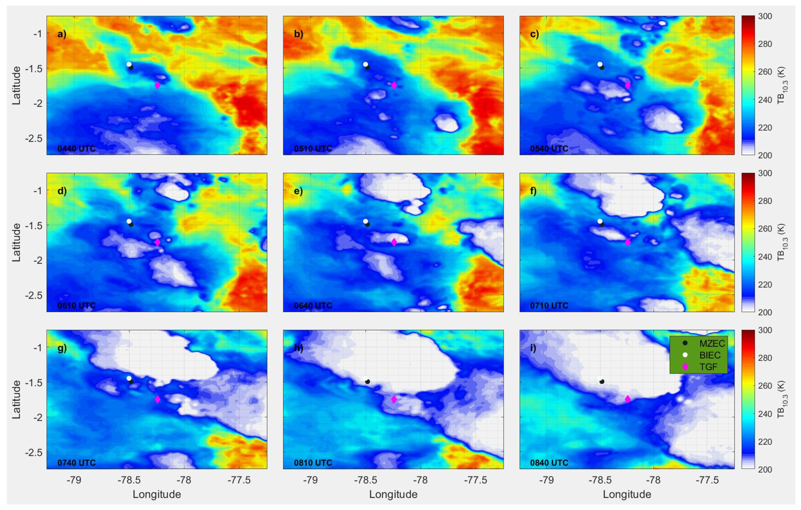
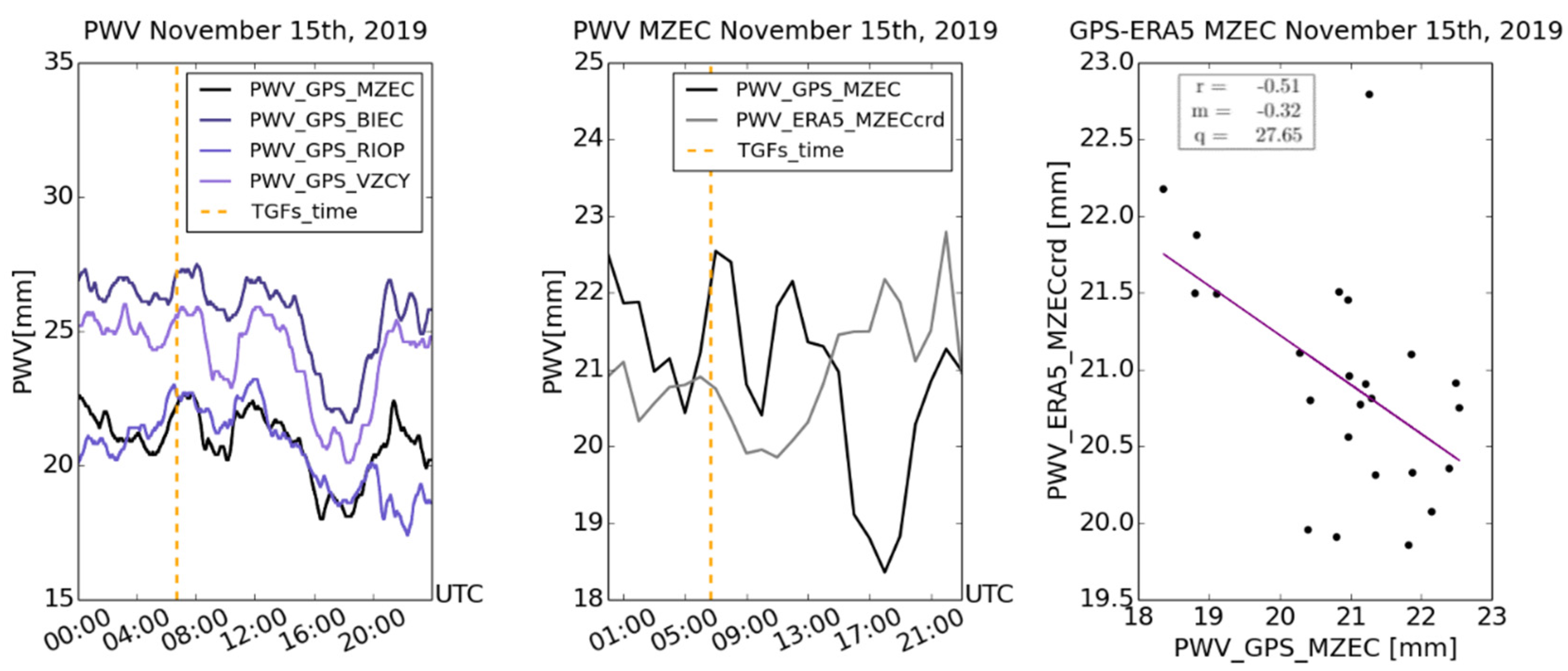
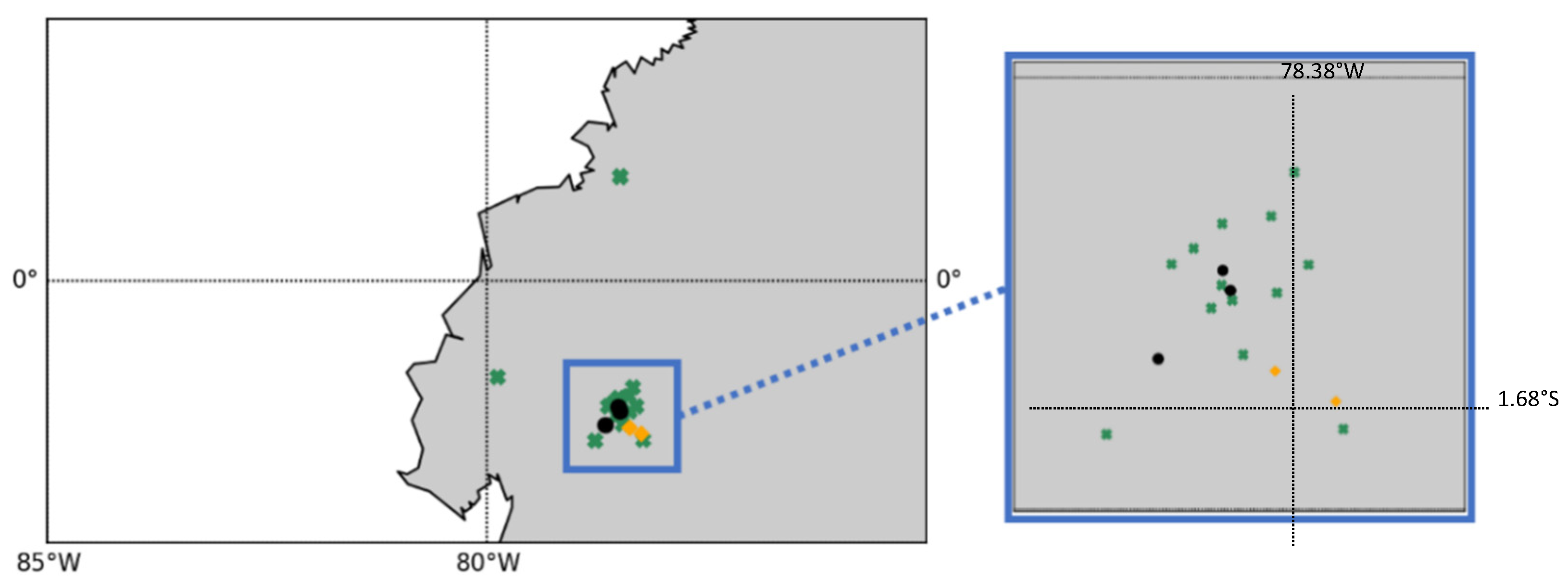
3.2.2. Ecuador—15 November 2019

This second case study considers an event that occurred over the mountains of Ecuador on 15 November 2019. Two TGFs, very close in time and space to each other (slightly more than one minute difference and around 19 km apart), were recorded for this event. In this case, four GPS receivers are available at different distances, MZEC, BIEC, RIOP and VZCY (see Table 2).

Figure 11a is the same as Figure 6 except that the data were collected by the GOES-R satellite. The sequence of satellite images, starting 2 hours before the TGF occurrence (Figure 6a), shows the same features as the previous case, highlighting the development of the convective cell that will generate the TGF. The TBs reported in Figure 11e (i.e., the GOES-R image closest to the TGF time) show very deep convection with values up to 205 K, even if the spatial extension of the convective cloud is quite limited, especially if compared to the convective cells covering the area.

In this case, the TGFs are both located at the edge of the convective cell (one on the southern edge and one on the north-western edge). For this case study, the comparison between GPS-PWV data and ERA5-PWV data showed a bad correlation with negative values of r (see Table 2). The complex topography affects the reliability of the ERA5 model and the patterns, obtained by the bias removal, showed great discrepancies with respect to the GPS-PWV (e.g., Figure 12, central and right panels considering the MZEC receiver). This point highlights the strong potential of the use of GPS data, for the troposphere characterization, in areas with complex territorial morphologies. Furthermore, the PWV trends for the four GPS receivers are very similar to each other (except more marked differences at the end of the day), even if the absolute values change depending on the altitude of the GPS receivers. In Figure 13, the distribution of pierce points (PPs) referred to the MZEC GPS receiver is shown. Further, in this case, the PPs are well distributed nearby both the GPS receivers and TGFs. This implies that the GPS-PWV trend (Figure 12, left panel) results as being particularly useful and reliable for the analysis of the event. It has to be highlighted that because of the vicinity in space and time of the two TGFs, the analysis was performed taking as refence only one out of the two TGFs.

The combined analysis of GPS-PWV for the MZEC site and the stroke rate trend (Figure 14) shows very similar features to the previous case study. In particular, the TGFs occurred slightly before both the second stroke rate maximum and the PWV maximum. For this event, the stroke rate has higher values, exceeding 20 strokes/min.

4. Discussion and Conclusions

In order to characterize the environmental and the cloud properties associated with the generation of a TGF, a total of 648 events detected by AGILE MCAL were analyzed. The investigation of the atmospheric conditions at the TGF occurrences with ERA5 reanalyses shows that TGFs mainly occur in convective environments. However, the values of meteorological parameters describing the convective environment are not exceptional. The CAPE measured in correspondence with a TGF occurrence does not show any particular variation with respect to the monthly average in the same location. This result is in agreement with the results obtained from the analysis over 24 TGF-producing storms conducted by [12]. On the other hand, the high values of CIN, TCWV and T2D measured at the TGF occurrence are indicative of the fact that they occur preferentially when the updrafts reach their maximum development. The time evolution of these convective systems was investigated by using the geostationary data, which are useful to describe the development of the storm. The life cycle of the storm (from the early stages to its mature phase) through a sequence of nine geostationary satellite snapshots shows how, at the TGF time, the cloud top reaches its maximum height with temperatures dropping down to about 200 K for the totality of the observed events. These results are in agreement with [14], where both space-borne active and passive microwave sensors agree in describing TGF-producing clouds as intense thunderstorms, with the presence of convective towers. Within the analyzed structures, however, the cloud top topography shows a wide range of extensions and the TGF is located at the edge of the convective cell.

A more in-depth characterization of the atmospheric conditions at the TGF occurrence was made possible by the analysis of PWV as estimated by the GPS sensors and by the ERA5 dataset. The comparison between GPS-PWV and ERA5-PWV data, for a number of case studies characterized by different topographical conditions, showed a very good correlation in the case of low-altitude sites and a bad correlation where orography is impactful. The analysis shows the strong potential of the use of GPS data for the troposphere characterization in areas with complex territorial morphologies. Furthermore, the focus on the distribution of PPs with respect to GPS receivers shows that the PPs are well distributed around the GPS devices and close to the TGF location. Therefore, the GPS-PWV trend can be considered well representative of the water vapor content within the areas of TGF occurrences. In all the analyzed case studies, the time of the TGF is within the maximum convection phase. Moreover, comparing the GPS-PWV trend with the ERA5-PWV trend at TGF coordinates, a slight offset between GPS-PWV and ERA5-PWV curves is detectable, which is related to the structure of the convective clouds and to the position of GPS sensors in relation to TGF coordinates.

The combined use of GPS and the stroke rate trends shows, for the two case studies shown in the text, an increase of PWV about two hours before the TGF. This trend is generally confirmed also considering all the case studies considered. TGFs occurred before or during the lightning peak and in correspondence with the local or absolute maximum PWV. These results suggest that the TGF occurrence and the flash rate trend are consistent with what was shown in [10,11], highlighting that a TGF often occurs during the most lightning-active phase of the storm. Moreover, the relation between PWV and the lightning trend is in agreement with [20], where PWV starts rising from 2 to 3 h before the peak of lightning activity. The lightning flash rate distribution exhibited high values (16 and 20 flashes/min), compared with [11], where 50% of events showed a flash rate less than 5 flashes/5 min with a maximum reference value of 40 flashes/5 min.

It is worth noting that the sample presented in this work is global, including regions with a very low WWLLN detection efficiency, more prone to a bias towards large-scale convective systems with extended lightning activity and more easily detectable. We point out that this is an unavoidable bias affecting every global TGF sample requiring a lightning association, which is also reported in [8,9,11].

References

1. Fishman, G.J. Discovery of Intense Gamma-Ray FLashes of Atmospheric Origin. Science 1994, 264, 1313–1316. [Google Scholar] [CrossRef] [PubMed] [Green Version]
2. Dwyer, J.R. The relativistic feedback discharge model of terrestrial gamma ray flashes. J. Geophys. Res. Space Phys. 2012, 117, 117. [Google Scholar] [CrossRef]
3. Smith, D.M. Terrestrial Gamma-Ray FLashes Observed up to 20 MeV. Science 2005, 307, 1085–1088. [Google Scholar] [CrossRef] [Green Version]
4. Briggs, M.S.; Fishman, G.J.; Connaughton, V.; Bhat, P.N.; Paciesas, W.S.; Preece, R.D. First Results on Terrestrial Gamma-ray Flashes from the Fermi Gamma-ray Burst Monitor. J. Geophys. Res. 2010, 115, A7. [Google Scholar] [CrossRef]
5. Marisaldi, M.; Fuschino, F.; Labanti, C.; Galli, M.; Longo, F.; Del Monte, E.; Barbiellini, G.; Tavani, M.; Giuliani, A.; Moretti, E.; et al. Detection of terrestrial gamma ray flashes up to 40 MeV by the AGILE satellite. J. Geophys. Res. Space Phys. 2010, 115. [Google Scholar] [CrossRef]
6. Neubert, V.T.; Østgaard, N.; Blanc, E.; Chanrion, O.; Oxborrow, C.A.; Orr, A.; Tacconi, M.; Hartnack, O.; Bhanderi, D.D.V. The ASIM Mission on the International Space Station. Space Sci. Rev. 2019, 6, 254–273. [Google Scholar] [CrossRef] [Green Version]
7. Tavani, M.; Argan, A.; Paccagnella, A.; Pesoli, A.; Palma, F.; Gerardin, S.; Bagatin, M.; Trois, A.; Picozza, P.; Benvenuti, P.; et al. Possible effects on avionics induced by terrestrial gamma-ray flashes. Nat. Hazards Earth Syst. Sci. 2013, 13, 1127–1133. [Google Scholar] [CrossRef] [Green Version]
8. Splitt, M.E.; Lazarus, S.M.; Barnes, D.; Dwyer, J.R.; Rassoul, H.K.; Smith, D.M. Thunderstorm Characteristics Associated with RHESSI Identified Terrestrial Gamma Ray FLashes. J. Geophys. Res. Atmos. 2010, 115, 6. [Google Scholar] [CrossRef]
9. Smith, D.M. Terrestrial Gamma Ray FLashes Correlated to Storm Phase and Tropopause Height. J. Geophys. Res. Space Phys. 2010, 115, 86–88. [Google Scholar] [CrossRef] [Green Version]
10. Tiberia, A.; Dietrich, S.; Porcù, F.; Marisaldi, M.; Ursi, A.; Tavani, M. Gamma ray storms: Preliminary meteorological analysis of AGILE TGFs. Rend. Lincei. Sci. Fis. Nat. 2019. [Google Scholar] [CrossRef]
11. Ursi, A.; Marisaldi, M.; Dietrich, S.; Tavani, M.; Tiberia, A.; Porcù, F. Analysis of Thunderstorms Producing Terrestrial Gamma Ray Flashes with the Meteosat Second Generation. J. Geophys. Res. Atmos. 2019, 124, 12667–12682. [Google Scholar] [CrossRef]
12. Chronis, T.; Briggs, M.S.; Priftis, G.; Connaughton, V.; Brundell, J.; Holzworth, R.; Heckman, S.; McBreen, S.; Fitzpatrick, G.; Stanbro, M. Characteristics of Thunderstorms That Produce Terrestrial Gamma Ray Flashes. Bull. Am. Meteorol. Soc. 2016, 97, 639–653. [Google Scholar] [CrossRef]
13. Mesinger, F.; DiMego, G.; Kalnay, E.; Mitchell, K.; Shafran, P.C.; Ebisuzaki, W.; Jović, D.; Woollen, J.; Rogers, E.; Berbery, E.H.; et al. North American Regional Reanalysis. Bull. Am. Meteorol. Soc. 2006, 87, 343–360. [Google Scholar] [CrossRef] [Green Version]
14. Tiberia, A.; Porcú, F.; Marisaldi, M.; Ursi, A.; Fuschino, F.; Tavani, M.; Dietrich, S. GPM-DPR Observations on TGFs Producing Storms. Press 2020. [Google Scholar] [CrossRef]
15. Hou, A.Y.; Kakar, R.K.; Neeck, S.; Azarbarzin, A.A.; Kummerow, C.D.; Kojima, M.; Oki, R.; Nakamura, K.; Iguchi, T. The Global Precipitation Measurement Mission. Bull. Am. Meteorol. Soc. 2014, 95, 701–722. [Google Scholar] [CrossRef]
16. Price, C. Lightning and Climate: The Water Vapor Connection; American Geophysical Union: Washington, DC, USA, 2001. [Google Scholar]
17. Bevis, M.; Businger, S.; Herring, T.A.; Rocken, C.; Anthes, R.A.; Ware, R.H. GPS meteorology: Remote sensing of atmospheric water vapor using the global positioning system. J. Geophys. Res. Space Phys. 1992, 97, 15787–15801. [Google Scholar] [CrossRef]
18. Duan, J.; Bevis, M.; Fang, P.; Bock, Y.; Chiswell, S.; Businger, S. GPS Meteorology: Direct Estimation of the Absolute Value of Precipitable Water. J. Appl. Meteorol. 1996, 35, 830–838. [Google Scholar] [CrossRef] [Green Version]
19. Inoue, H.Y.; Inoue, T. Characteristics of the Water-Vapor Field over the Kanto District Associated with Summer Thunderstorm Activities. SOLA 2007, 3, 101–104. [Google Scholar] [CrossRef] [Green Version]
20. D’Adderio, L.P.; Pazienza, L.; Mascitelli, A.; Tiberia, A.; Dietrich, S. A Combined IR-GPS Satellite Analysis for Potential Applications in Detecting and Predicting Lightning Activity. Remote Sens. 2020, 12, 1031. [Google Scholar] [CrossRef] [Green Version]
21. Marisaldi, M.; Fuschino, F.; Tavani, M.; Dietrich, S.; Price, C.; Galli, M. Properties of Terrestrial Gamma Ray FLashes Detected by AGILE MCAL below 30 MeV. J. Geophys. Res. Space Phys. 2014, 119, 1337–1355. [Google Scholar] [CrossRef]
22. Lindanger, A.; Marisaldi, M.; Maiorana, C.; Sarria, D.; Albrechtsen, K.; Østgaard, N.; Galli, M.; Ursi, A.; Labanti, C.; Tavani, M.; et al. The 3rd AGILE terrestrial gamma ray flash catalog. Part I: Association to lightning sferics. J. Geophys. Res. Atmos. 2020, 125, e2019JD031985. [Google Scholar] [CrossRef]
23. Maiorana, C.; Marisaldi, M.; Lindanger, A.; Østgaard, N.; Ursi, A.; Sarria, D.; Galli, M.; Labanti, C.; Tavani, M.; Pittori, C.; et al. The 3rd AGILE Terrestrial Gamma-ray Flashes Catalog. Part II: Optimized Selection Criteria and Characteristics of the New Sample. J. Geophys. Res. Atmos. 2020, 125. [Google Scholar] [CrossRef]
24. Tavani, M. The AGILE Mission. Astron. Astrophys. 2009, 502, 995–1013. [Google Scholar] [CrossRef]
25. Labanti, C. Design and Construction of the Mini-Calorimeter of the AGILE Satellite. Nucl. Instrum. Methods Phys. Res. 2009, 598, 470–479. [Google Scholar] [CrossRef] [Green Version]
26. Marisaldi, M.; Argan, A.; Ursi, A.; Gjesteland, T.; Fuschino, F.; Labanti, C.; Galli, M.; Tavani, M.; Pittori, C.; Verrecchia, F.; et al. Enhanced detection of terrestrial gamma-ray flashes by AGILE. Geophys. Res. Lett. 2015, 42, 9481–9487. [Google Scholar] [CrossRef] [PubMed] [Green Version]
27. Hutchins, M.L.; Holzworth, R.H.; Brundell, J.B.; Rodger, C.J. Relative detection efficiency of the World Wide Lightning Location Network. Radio Sci. 2012, 47. [Google Scholar] [CrossRef]
28. Connaughton, V.; Briggs, M.S.; Xiong, S.; Dwyer, J.R.; Hutchins, M.L.; Grove, J.E. Radio Signals from Electron Beams in Terrestrial Gamma Ray Flashes. J. Geophys. Res. Space Phys. 2013, 118, 2313–2320. [Google Scholar] [CrossRef] [Green Version]
29. Groves, P.D. Principles of GNSS, inertial, and multisensor integrated navigation systems, 2nd edition [Book review]. IEEE Aerosp. Electron. Syst. Mag. 2015, 30, 26–27. [Google Scholar] [CrossRef]
30. Sansò, F. Navigazione Geodetica e Rilevamento Cinematico; Polipress: Roma, Italy, 2006. [Google Scholar]
31. Sampietro, D.; Caldera, S.; Capponi, M.; Realini, E. Geoguard-An Innovative Technology Based on Low-Cost GNSS Receivers to Monitor Surface Deformations. In Proceedings of the First EAGE Workshop on Practical Reservoir Monitoring, European Association of Geoscientists & Engineers, Amsterdam, The Netherlands, 6–9 March 2017; p. cp-505. [Google Scholar]
32. Mascitelli, A.; Coletta, V.; Bombi, P.; De Cinti, B.; Federico, S.; Matteucci, G.; Mazzoni, A.; Muzzini, V.G.; Petenko, I.; Dietrich, S. Tree Motion: Following the Wind-Induced Swaying of Arboreous Individual Using a GNSS Receiver. Ital. J. Agrometeorol. 2019, 3, 25–36. [Google Scholar]
33. Fratarcangeli, F.; Savastano, G.; D’Achille, M.C.; Mazzoni, A.; Crespi, M.; Riguzzi, F.; DeVoti, R.; Pietrantonio, G. VADASE Reliability and Accuracy of Real-Time Displacement Estimation: Application to the Central Italy 2016 Earthquakes. Remote. Sens. 2018, 10, 1201. [Google Scholar] [CrossRef] [Green Version]
34. Mascitelli, A. New Applications and Opportunities of GNSS Meteorology. Ph.D. Thesis, Sapienza Università di Roma, Roma, Italy, 2020. [Google Scholar]
35. Mascitelli, A.; Federico, S.; Torcasio, R.C.; Dietrich, S. Assimilation of GPS Zenith Total Delay Estimates in RAMS NWP Model: Impact Studies over Central Italy. Adv. Space Res. 2020. [Google Scholar] [CrossRef]
36. Campanelli, M.; Mascitelli, A.; Sanò, P.; Diémoz, H.; Estellés, V.; Federico, S.; Iannarelli, A.M.; Fratarcangeli, F.; Mazzoni, A.; Realini, E. Precipitable Water Vapour Content from ESR/SKYNET Sun–Sky Radiometers: Validation against GNSS/GPS and AERONET over Three Different Sites in Europe. Atmos. Meas. Tech. 2018, 11, 81. [Google Scholar] [CrossRef] [Green Version]
37. Saastamoinen, J. Contributions to the Theory of Atmospheric Refraction. Bull. Géod. 1946–1975 1973, 107, 13–34. [Google Scholar] [CrossRef]
38. Hopfield, H. Two-Quartic Tropospheric Refractivity Profile for Correcting Satellite Data. J. Geophys. Res. 1969, 74, 4487–4499. [Google Scholar] [CrossRef]
39. Realini, E.; Sato, K.; Tsuda, T.; Manik, T. An Observation Campaign of Precipitable Water Vapor with Multiple GPS Receivers in Western Java, Indonesia. Prog. Earth Planet. Sci. 2014, 1, 17. [Google Scholar] [CrossRef] [Green Version]
40. Berberan-Santos, M.N.; Bodunov, E.N.; Pogliani, L. On the Barometric Formula. Am. J. Phys. 1997, 65, 404–412. [Google Scholar] [CrossRef]
41. Bai, Z.; Feng, Y. GPS Water Vapor Estimation Using Interpolated Surface Meteorological Data from Australian Automatic Weather Stations. J. Glob. Position. Syst. 2003, 2, 83–89. [Google Scholar] [CrossRef]
42. Böhm, J.; Heinkelmann, R.; Schuh, H. Short Note: A Global Model of Pressure and Temperature for Geodetic Applications. J. Geod. 2007, 81, 679–683. [Google Scholar] [CrossRef]
43. Hersbach, H. The ERA5 Atmospheric Reanalysis. AGUFM 2016, 2016, NG33D-01. [Google Scholar]
44. Zumberge, J.F.; Heflin, M.B.; Jefferson, D.C.; Watkins, M.M.; Webb, F.H. Precise Point Positioning for the Efficient and Robust Analysis of GPS Data from Large Networks. J. Geophys. Res. Solid Earth 1997, 102, 5005–5017. [Google Scholar] [CrossRef] [Green Version]
45. Herrera, A.M.; Suhandri, H.F.; Realini, E.; Reguzzoni, M.; de Lacy, M.C. GoGPS: Open-Source MATLAB Software. GPS Solut. 2016, 20, 595–603. [Google Scholar] [CrossRef]
46. Schmit, T.J.; Griffith, P.; Gunshor, M.M.; Daniels, J.M.; Goodman, S.J.; Lebair, W.J. A Closer Look at the ABI on the GOES-R Series. Bull. Am. Meteorol. Soc. 2017, 98, 681–698. [Google Scholar] [CrossRef]
47. Schmit, T.J.; Gunshor, M.M.; Menzel, W.P.; Gurka, J.J.; Li, J.; Bachmeier, A.S. Introducing the next-generation advanced baseline imager on GOES-R. Bull. Am. Meteorol. Soc. 2005, 86, 1079–1096. [Google Scholar] [CrossRef]
48. Bessho, K.; Date, K.; Hayashi, M.; Ikeda, A.; Imai, T.; Inoue, H. An Introduction to Himawari 8/9 Japan’s New-Generation Geostationary Meteorological Satellites. J. Meteorol. Soc. Jpn. 2016, 94, 151–183. [Google Scholar] [CrossRef] [Green Version]
49. Iwabuchi, H.; Putri, N.S.; Saito, M.; Tokoro, Y.; Sekiguchi, M.; Yang, P.; Baum, B.A. Cloud Property Retrieval from Multiband Infrared Measurements by Himawari-8. J. Meteorol. Soc. Jpn. 2018, 27–42. [Google Scholar] [CrossRef] [Green Version]
50. Berrisford, P.; Kållberg, P.; Kobayashi, S.; Dee, D.; Uppala, S.; Simmons, A.J.; Poli, P.; Sato, H. Atmospheric conservation properties in ERA-Interim. Q. J. R. Meteorol. Soc. 2011, 137, 1381–1399. [Google Scholar] [CrossRef]
Figure 1. Geographical distribution of the 648 terrestrial gamma-ray flash (TGF) events with associated lightning sferics detected by the AGILE MCAL instrument between March 2015 and February 2020.
Remotesensing 13 00784 g001
Figure 2. Distributions of (a) longitude, (b) local time, (c) duration (t50) and (d) intensity for the selected TGF sample.
Remotesensing 13 00784 g002
Figure 3. Boxplot of the atmospheric parameters for TGF (brown bars) and reference values (transparent blue bars). The number of the months is along the x-axis. The 25th and 75th percentiles are shown by the boxes, while the maximum and minimum values are given by the error bars. The average is shown by a trait inside the boxes. (a) Convective available potential energy (CAPE) [J\Kkg]; (b) convection inhibition energy (CIN) [J\Kkg]; (c) total column water vapor (TCWV) [mm]; and (d) 2 m dew point temperature (T2D) [K].
Remotesensing 13 00784 g003
Figure 4. Indonesian case studies. GPS receivers (black dots) and TGFs’ (orange diamonds) positions. Green square—case study Sumatra, 16 March 2019.
Remotesensing 13 00784 g004
Figure 5. American case studies. GPS receivers (black dots) and TGFs’ (orange diamonds) positions. Green square—case study Ecuador, 15 November 2019.
Remotesensing 13 00784 g005
Figure 6. Snapshots of brightness temperature (TB) at 10.3 µm from Himawari-8 satellite from 08:30 UTC to 12:30 UTC on 16 March 2019 within a 2° × 2° area centered at the TGF location near the coast of Sumatra. The black dot indicates the TGF location, while the diamonds indicate the GPS receivers’ locations. The panel (e) corresponds to the instant closest to the TGF occurrence.
Remotesensing 13 00784 g006
Figure 7. GPS-precipitable water vapor (PWV) data and ERA5-PWV data referred to LNNG GPS receiver, on 16 March 2019, Sumatra TGF case. In the right panel, r is the correlation coefficient, m is the slope and q is the intercept.
Remotesensing 13 00784 g007
Figure 8. GPS-PWV data and ERA5-PWV data referred to MKMK GPS receiver, on 16 March 2019, Sumatra TGF case. In the right panel, r is the correlation coefficient, m is the slope and q is the intercept.
Remotesensing 13 00784 g008
Figure 9. Distribution of pierce points, at 7 km of altitude, referred to LNNG GPS receiver. GPS receivers (black dots), TGF position (orange diamonds) and pierce points’ positions (green crosses)—case study 16 March 2019, Sumatra TGF case.
Remotesensing 13 00784 g009
Figure 10. Daily trend of GPS-PWV (black solid line) and stroke rate (blue solid line). The vertical dashed line indicates the time of TGF occurrence—case study 16 March 2019, Sumatra TGF case.
Remotesensing 13 00784 g010
Figure 11. Snapshots of TB at 10.3 µm from GOES-R satellite from 04:40 UTC to 08:40 UTC on 15 November 2019 within a 2° × 2° area centered at the TGF location in Ecuador. The diamonds indicate the TGFs’ locations, while the dots indicate the GPS receivers’ locations. The panel (e) corresponds to the instant closest to the TGF occurrence.
Remotesensing 13 00784 g011
Figure 12. GPS-PWV data referred to GPS receivers, on 15 November 2019, Ecuador TGF case. The first panel shows the PWV values referred to the GPS sensors located in the vicinity of TGF coordinates; in the central panel, the comparison between GPS-PWV and ERA5-PWV related to one of GPS receivers (MZEC) is given; and in the third one, the correlation between GPS-PWV and ERA5-PWV is shown. In the right panel, r is the correlation coefficient, m is the slope and q is the intercept.
Remotesensing 13 00784 g012
Figure 13. Distribution of pierce points, at 7 km of altitude, referred to MZEC GPS receiver. GPS receivers (black dots), TGFs’ positions (orange diamonds) and pierce points’ positions (green crosses)—case study 15 November 2019, Ecuador TGF case.
Remotesensing 13 00784 g013
Figure 14. Daily trend of GPS-PWV (black solid line) and stroke rate (blue solid line). The vertical dashed line indicates the time of TGF occurrence—15 November 2019, Ecuador TGF case.
Remotesensing 13 00784 g014